Shear Thinning in the Prandtl Model and Its Relation to Generalized Newtonian Fluids

Abstract

The Prandtl model is certainly the simplest and most generic microscopic model describing solid friction. It consists of a single, thermalized atom attached to a spring, which is dragged past a sinusoidal potential representing the surface energy corrugation of a counterface. While it was primarily introduced to rationalize how Coulomb’s friction law can arise from small-scale instabilities, Prandtl argued that his model also describes the shear thinning of liquids. Given its success regarding the interpretation of atomic-force-microscopy experiments, surprisingly little attention has been paid to the question how the Prandtl model relates to fluid rheology. Analyzing its Langevin and Brownian dynamics, we show that the Prandtl model produces friction–velocity relationships, which, converted to a dependence of effective (excess) viscosity on shear rate $\eta \left(\dot{\gamma }\right)$, is strikingly similar to the Carreau–Yasuda (CY) relation, which is obeyed by many non-Newtonian liquids. The two dimensionless parameters in the CY relation are found to span a broad range of values. When thermal energy is small compared to the corrugation of the sinusoidal potential, the leading-order ${\dot{\gamma }}^2$ corrections to the equilibrium viscosity only matter in the initial part of the cross-over from Stokes friction to the regime, where $\eta$ obeys approximately a sublinear power law of $1/\dot{\gamma }$.

1. Introduction

Understanding frictional forces and thus energy dissipation between two sliding bodies is a central task of tribology. The Prandtl model is arguably the simplest and most generic non-linear model explaining why and how energy dissipates microscopically [1,2,3]. It consists of a mass point, which is dragged by a spring of stiffness k past a corrugated potential and subjected to a Stokesian drag force as well as to thermal fluctuations. When k is less than the maximum curvature of the potential $V_{\max }^{″}$, instabilities occur and friction has a finite zero-velocity limit in the absence of thermal noise, consistent with Coulomb’s law of friction. When thermal fluctuations are minor and velocities are intermediate, the dependence of friction on velocity can be rather weak, again consistent with the observations going back to Coulomb [4], who never claimed solid friction to be completely independent of velocity. However, if the reduced spring stiffness $\tilde{k}\equiv k/V_{\max }^{″}>1$ and/or when the thermal energy $k_{B}T$ is finite, the dependence of the friction force F on velocity v is Stokesian at small v but usually much enhanced compared to that caused by the artificially added damping term.

The Prandtl model—while having been mistakenly attributed to Tomlinson, see the interesting summary by Popov and Gehrt [3] preceding their translation of Prandtl’s original work—received a revival when it was realized that the model (sometimes with minor modifications) can quantitatively describe friction and stick–slip dynamics as measured in atomic-force-microscope experiments [5,6,7,8,9,10]. This includes the transition between stick–slip motion [11] and structural lubricity [12] upon a decrease of load, i.e., the regime where solid friction turns into viscous friction. The relevance of the Prandtl model to fluid rheology remained nevertheless relatively unexplored, despite few exceptions [13,14]. This is surprising in light of Prandtl’s comment that we obtain the complete transition from solid bodies to liquids of low viscosity including all states of softening in between. (Here, and in the following, quotations set in italic refer to the excellent English translation by Popov and Gray [3] rather than to the original German.) Moreover, Prandtl expected viscosity $\eta$ to increase (only approximately) exponentially with pressure p, in agreement with the so-called Barus equation, its generalizations, and more recent experiments [14,15,16] as well as molecular simulations [17].

Simple microscopic models describing shear-thinning in non-Newtonian liquids properly are scarce if existent at all. The most standard model, which could be called semi-phenomenological, is the Eyring model [14,16,18,19], which assumes the existence of a single energy barrier opposing (lateral) motion of an atom when a fluid is sheared. The Eyring model arises as the limiting $\tilde{k}\to 0$ case of the Prandtl model. The dependence of (excess) viscosity $\eta$ on shear rate $\dot{\gamma }$ in the Eyring model is given by

$$\eta \left(\dot{\gamma }\right)={\eta }_{\mathrm{N}}\frac{{\dot{\gamma }}_0}{\dot{\gamma }}\mathrm{arsinh}\left(\frac{\dot{\gamma }}{{\dot{\gamma }}_0}\right),$$

(1)

where ${\eta }_{\mathrm{N}}$ is the equilibrium (excess) viscosity and ${\dot{\gamma }}_0$ a characteristic shear rate near which friction crosses over from a linear, fluid-like to a quasi-logarithmic, solid-like dependence on velocity. The term “excess” is meant to indicate that experimental results on “full” viscosities, i.e., ratios of shear stresses and shear rates, are often fit to equations of the form ${\eta }_{\mathrm{full}}\left(\dot{\gamma }\right)={\eta }_{\infty }+\eta \left(\dot{\gamma }\right)$. In the following, the contribution ${\eta }_{\infty }$ is ignored and we content ourselves with the comment that a related term arises in the Prandtl model when an explicit Stokesian damping acts between the mass point and the substrate.

While many liquids follow Eyring’s model at small temperatures or high pressure, a variety of phenomenological models are used in practice that assume a different functional dependence of viscosity on shear rate from Eyring. One such equation, which contains many other models as limiting cases, is the Carreau–Yasuda (CY) equation [20,21,22]

$$\eta \left(\dot{\gamma }\right)=\frac{{\eta }_{\mathrm{N}}}{{\left\{1+{(\dot{\gamma }/{\dot{\gamma }}_0)}^a\right\}}^{(1-n)/a}}$$

(2)

where n and a are dimensionless parameters. For example, the CY model reduces to the Carreau model for $a=2$, whereas the friction–shear rate dependence becomes logarithmic-like at large shear rates, as in the Eyring model, when n approaches zero from above. For ${\dot{\gamma }}_0\to 0$, viscosity is an algebraic function of shear rate, $\eta \left(\dot{\gamma }\right)\propto {\dot{\gamma }}^{n-1}$, so that shear stress increases sub-linearly with ${\dot{\gamma }}^n$ with an exponent $0<n<1$.

One drawback of the CY equation is that it cannot be asymptotically correct for very small velocities, except in the $a=2$ limit of the Carreau equation. The reason is that any rigorous, perturbation-theory approach to the finite-temperature statistical mechanics of sheared, originally isotropic liquids, in which the sliding velocity or shear rate is taken as small parameter, can only lead to a shear stress that can be expanded as odd powers of the shear rate. Such an expansion would hold up to the point at which the sheared liquid undergoes a (macroscopic) discontinuous change, whereby analyticity is destroyed. Consequently, it should be generally possible to express the effective viscosity as a Taylor series expansion in even powers of $\dot{\gamma }$, at least until a shear-driven thermodynamic phase transformation or another collective, symmetry-breaking phenomena occurs. The Eyring model obeys this principle, since the r.h.s. of Equation (1) can be expanded into even powers of $\dot{\gamma }$. The predicted friction–velocity relations can be systematically improved by adding further odd-power $\mathrm{arsinh}(\dot{\gamma }/{\dot{\gamma }}_0)$ terms, as shown in the context of the Prandtl model [13]. However, in preparing this work it was found that convergence tends to be slow in such an $\mathrm{arsinh}(\dot{\gamma }/{\dot{\gamma }}_0)$ expansion.

Although the CY equation violates elementary symmetry considerations, it certainly provides a quite reasonable description of many experiments, most notably those on polystyrene by Yasuda [21], which prompted Yasuda to generalize the Carreau equation; the data are reprinted (Figure 4.1-3) in the classical book by Bird, Armstrong, and Hassager on the dynamics of polymeric liquids [22]. An interesting aspects of the original results is that they are best described with the exponents $n=0.2$ and $a=1.25$. It means that, on the one hand, the experimental data show an almost Eyring/logarithmic-like dependence of shear stress at intermediate sliding velocities since $n=0.2$ is much closer to zero than to unity. On the other hand, the parameter a clearly differs from the value of two in violation of a leading-order $\eta \left(\dot{\gamma }\right)=\eta \left(0\right)+{\eta }^{″}\left(0\right){\dot{\gamma }}^2/2$ dependence. which would be consistent with perturbation theory or Eyring.

The initial motivation for the current study was to address the question of whether simulations can reproduce experimental results that appear to violate elementary symmetry considerations and to analyze the system with high precision at exceedingly small shear rates within the linear-response regime. Such a study will also implicitly address the question of how a shear-stress dependent effective (free) energy barrier $F\left(\tau \right)$, which is defined through the equation

$$\dot{\gamma }\left(\tau \right)=\frac{\tau }{{\eta }_{\mathrm{N}}}{e}^{-\beta \left\{F\right(\tau )-F(0\left)\right\}},$$

(3)

depends on shear stress $\tau$. Generally speaking, the leading-order correction to any finite-temperature free-energy barrier $\Delta F\left(\tau \right)=F\left(\tau \right)-F\left(0\right)$, including those opposing a chemical reaction, to an external stress can only be an analytical function in the stress tensor invariants, e.g., the hydrostatic pressure p and the deviatoric stress tensor invariant, which can be associated with the square of the shear stress. Thus, tensile stress $\sigma$ can change $\Delta F$ in leading linear order, since it couples linearly to the hydrostatic pressure, but the leading-order correction to $\Delta F\left(\tau \right)$ can only be quadratic in shear stress except at zero temperature, where analyticity does not necessarily hold. In addition, the notion of an activation volume when expressing the seemingly linear reduction of a finite-temperature free-energy barrier with respect to shear stress appears particularly troublesome as a (Lagrangian) shear strain leaves the volume unchanged.

The symmetry arguments on free-energy barriers appear to be in conflict with the assumption of an athermal energy barrier $\Delta E$ that decreases linearly rather than quadratically with shear stress and which is used in transition-state theory [14]. A similar comment applies to other energy barriers that can be reduced by shear stress, such as those opposing chemical reactions. Strong support for a linear reduction of activation energies comes from the shear-stress assisted decomposition of zinc-phosphate based anti-wear additives immersed in sheared, highly viscous lubricants [23].

To study the conditions if/when free-energy barriers depend linearly or quadratically on shear stress, very high-precision, effective viscosities are required at small shear rates. Computing them in explicit many-atom simulations with sufficient precision might require unfeasible computing times even for model substances as simple as liquid Lennard–Jonesium. It was therefore decided to investigate the Prandtl model. Discovering that and rationalizing why it mimics the shear thinning of real liquids—which we now consider the main message of this paper—was a coincidental byproduct of the attempt to reconcile symmetry arguments with empirical evidence.

A frequent advantage of studying simple systems is that some of the gained insights apply to a broader context than simulations of just one specific substance. This happens when the description of complex, seemingly unrelated systems simplifies to the same unifying model after abstracting the effects of irrelevant degrees of freedom into a thermostat. Thus, liquids with rheological responses as distinct as those of polystyrene and camel’s blood may be describable by the same, simple model. This simplification is particularly/only useful, if it allows questions such as why increasing the pressure of an ordinary liquid or decreasing the stiffness of red blood cells leads to a decrease of the exponent n in the CY model to be answered.

The remainder of this article is organized as follows: Section 2 presents the investigated model, some theory as well as a brief discussion of the numerical methods used. Section 3 contains the results. Conclusions are drawn in Section 4.

2. Model, Theory, and Methods

In this section, we first describe the Prandtl model in a slightly modified form, that is, the explicitly introduced damping of the mass point does not occur relative to the substrate but within the spring. The three different methods pursued to study the dynamics of the system are also described in this section. The numerical methods include: molecular dynamics using a Langevin thermostat for the study of underdamped dynamics as well as Brownian dynamics and a Fokker–Planck-equation based approach for the simulation of overdamped dynamics. Since the Brownian dynamics and the Fokker–Planck equation are not commonly used in the field of tribology, despite notable exceptions [24,25], some technical details on these methods are reported in the following.

2.1. The Prandtl Model

A variant of the Prandtl model is chosen in which the mass point’s velocity is damped with respect to the driving spring, i.e., the equation of motion in the frame of reference of the moving spring reads

$$m\ddot{x}+m\gamma \dot{x}+kx=q{V}_{0}sin(qx+v_{0}t)+\Gamma \left(t\right),$$

(4)

where m is the mass, $\gamma$ is a damping coefficient, k the stiffness of the driving spring, $V_0$ the amplitude of the substrate potential, and $2\pi /q$ is the spatial period. $\Gamma \left(t\right)$ is a random force mimicking thermal fluctuations and thus satisfying the fluctuation–dissipation theorem.

Damping was chosen to act relative to the driving spring for mainly two reasons. First, it automatically turns the measured friction force into an excess friction compared to that at infinitely large velocities, whereby postanalysis is facilitated. The reason that $F(v\to \infty )$ tends to zero is that the mass point is too inert, or in the overdamped limit too sluggish, to respond to the rapidly changing deterministic forces imposed by the substrate. Second, dissipation occurs within a linearly elastic system through the coupling of a single, atomistic degree of freedom to a quasi-continuous set of collective harmonic modes. For ideally elastic solids, the damping coefficient of a surface atom—as obtained within the Debye approximation to harmonic solids—is roughly half the eigenfrequency (see Equation (5.7) in [26]), which causes the motion of an individual surface atom to be slightly underdamped when described in terms of a harmonic coupling to its lattice site.

Results are sometimes expressed in a reduced system in which $m\gamma$, q, and $V_0$ as well as $k_B$ are all equal to unity. The remaining parameters of the Prandtl model are reduced velocity $\tilde{v}=vq/\gamma$, reduced mass $\tilde{m}=m/\sqrt{q^2{V}_0/{\gamma }^2}$, reduced thermal energy $k_B\tilde{T}=k_{B}T/V_0$, and most importantly reduced spring stiffness $\tilde{k}=k/\left(q^2{V}_0\right)$. In this unit system, the maximum, athermal static friction force is ${\tilde{F}}_{\mathrm{s},\max }=1$ in the limit of $\tilde{k}\to 0$, which would also be the maximum, athermal, zero-velocity kinetic friction force.

It may be helpful to note that the letter T can indicate both temperature and period $T=2\pi /\left(q{v}_0\right)$ for the lack of alternatives. To discriminate between the two, the letter $k_B$ precedes T or $\tilde{T}$, whenever the latter (letter) is meant to represent temperature but is omitted otherwise.

2.1.1. Relating the Prandtl Model to Rheology

To relate the Prandtl model to rheology, we consider laminar flow. Each Prandtl layer (in fact, Prandtl assumed many springs at irregular spacing so as to avoid artifacts due to commensurability) is assigned a width that is similar to the period of the substrate potential. Each layer also provides a corrugation potential to the next layer above it. Of course, the corrugation potential cannot be spatially periodic. However, as long as instabilities occur locally, only local potential-energy landscapes matter and these may be assumed to be similar to the used periodic function. Thus, if the center of mass of one layer slides at a velocity of $v_0$ with respect to its neighbor, the shear rate would be $\dot{\gamma }=v_0/(2\pi /q)$.

Following the picture described in the previous paragraph, a shear force in the Prandtl model can be associated with in a shear stress $\sigma$ after dividing the shear force by ${(2\pi /q)}^2$. Thus, a “real viscosity” of a liquid ${\eta }_{\mathrm{liq}}=\sigma /\dot{\gamma }$ and the velocity-dependent damping in the Prandtl model, ${\eta }_{\mathrm{P}}=F_{\mathrm{k}}/v_0$, are connected through the equation

$${\eta }_{\mathrm{liq}}=\frac{q{\eta }_{\mathrm{P}}}{2\pi }.$$

(5)

In the following, the symbol $\eta$ will refer exclusively to the damping in the Prandtl model, but we hope to have made clear its connection to viscosity.

2.1.2. Temperature Dependence of the Equilibrium Damping

As mentioned above, the Prandtl model reduces to the Eyring model for $\tilde{k}\to 0$, in which case a free, single particle moves through a sinusoidal potential under the influence of thermal noise and a constant drag force. This limit is well understood (see, for example, Risken’s excellent text book on the Fokker–Planck equation [27]). The small-velocity limit of the damping, which is also called Newtonian damping by analogy to Newtonian viscosity, can be deduced from the thermal diffusion constant D of the free particle through the Einstein–Smoluchowski relation $D=k_{B}T/\left(m\gamma \right)$. Since the diffusion in a corrugated potential is predominantly impeded by the energy barrier $2V_0$, diffusion of the free-particle is counteracted by an (inverse) Arrhenius factor of $exp\{2V_0/\left(k_{B}T\right)\}$. The missing prefactor can be estimated from the mobility of the free atom; the details and all complications arise from the fact that not only the energy barrier but also the entire energy landscape affect the atom’s final mobility and thus its damping constant.

We now discuss the evolution of the probability distribution $W(x,t)$ in the Prandtl model where $\tilde{k}$ is less than unity but still large enough for at most two minima in the total potential to occur at any given relative substrate position. (Allowing for more potential energy minima does not change final results in a significant fashion but requires a much longer discussion.) Moreover, assume that $k_B\tilde{T}\ll \Delta F(x_{\mathrm{s}}=0)$, where $x_{\mathrm{s}}=0$ indicates that the maximum of the substrate potential coincides with the spring’s equilibrium position, as depicted in Figure 1. When the substrate has not yet reached the situation shown in Figure 1 such that the left minimum is lower than the right by a few $k_{B}T$, essentially all the probability of $W(x,t)$ resides near the left minimum, i.e., near the one in which the dark blue atom is indicated. To what extent $W(x,t)$ has shifted to the right minimum when left and right minima are close to each other, say within less than $4k_{B}T$, depends crucially on the driving velocity $v_0$. In the limit $v_0\to 0$, the system is within the linear-response (Newtonian) regime and $W(x,t)$ is very close to the equilibrium distribution for a given substrate position, i.e., $W(x,t)\propto exp[-\beta V\{x,x_{\mathrm{s}}\left(t\right)\}]$. However, for this to occur, the mass point needs to equilibrate, i.e., it must overcome the barrier $\Delta F$ several times while the energy of the left minimum has been raised by a few $k_{B}T$ compared to the right. The corresponding time to do so increases with the Arrhenius factor $exp\{\Delta F/\left(k_{B}T\right)\}$, where $\Delta F$ is the energy barrier that has been renormalized from $2V_0$ due to the coupling of the (coarse-grained) atom to the spring, see again Figure 1. Assuming the prefactor of the equilibrium damping to be proportional to an inverse power of $k_{B}T$, we obtain

$$\tilde{\eta }={\left(\frac{k_B{\tilde{T}}_{\eta }}{k_B\tilde{T}}\right)}^{{\alpha }_{\eta }}{e}^{\Delta F/\left(k_B\tilde{T}\right)},$$

(6)

$k_B{\tilde{T}}_{\eta }$ and ${\alpha }_{\eta }$ being dimensionless parameters. The prefactor was added as a general power law of thermal energy, as to properly reflect, for example, under- and overdamped dynamics in the $\tilde{k}\to 0$ and $\tilde{k}\to \infty$ limits.

Another parameter affecting the linear damping coefficient is related to a characteristic distance that the spring can move relative to the substrate without significantly changing the energy landscape. It could be defined as the distance $\Delta X_{\mathrm{s}}$ from the symmetry point $X_{\mathrm{s}}=0$ that needs to be overcome to lift the degeneracy of the two minima by more than, say, $k_{B}T$. Alternatively, it might also be defined by the distance that needs to be slid until one of the two initially degenerate minima becomes unstable. Since the latter is independent of $k_{B}T$, we explore this distance graphically in Figure 2.

From Figure 2, it becomes obvious that the energy landscape for the larger $\tilde{k}$ value changes much more quickly than the smaller one. Specifically, at a slid distance $X_{\mathrm{s}}=0.01/q$, the energy landscape of the $\tilde{k}=0.85$ system has moved from being degenerate to the point where even an athermal mass point would move to the new absolute energy minimum. In contrast, the energy landscape of the $\tilde{k}=0.25$ system has barely changed when being slid by the same distance. To reach the point at which an athermal mass point would becomes unstable a distance roughly 80 times larger is needed for the softer spring. Thus, at fixed values of $\Delta E/k_{B}T$ and $q{v}_0$, the softer springs has more time to transit the barrier through thermal activation than the stiffer spring. Consequently, the equilibrium damping of the softer spring will be lower under these circumstances and its crossover velocity be greater than for the stiffer spring. This might be counterintuitive, since the athermal kinetic friction force in the $\tilde{v}\to 0$ limit is greater for the softer spring. The crude guesses from this section would be that the dimensionless equilibrium-damping term $\tilde{\eta }$ should be of order $exp(\beta \Delta F)$ (at least for the overdamped case, for the underdamped case a different unit system might be needed) and that the cross-over velocity for $\tilde{k}=0.25$ should exceed the crossover velocity for $\tilde{k}=0.85$ model by a factor whose order of magnitude is 80. Quantifying these numbers more accurately in terms of a closed-form analytical expression is beyond the scope of this work.

2.1.3. Shear-Stress Dependence of the Free-Energy Barrier

In the Eyring model, Equations (1) and (3) and the definition of the effective damping $\eta \equiv \tau /\dot{\gamma }$ can be combined to yield the following shear-stress dependence of the free-energy barrier

$$\Delta F\left(\tau \right)=\Delta F\left(0\right)-k_{B}Tlog\left(\frac{{\tau }_0}{\tau }sinh\frac{\tau }{{\tau }_0}\right),$$

(7)

where ${\tau }_0={\eta }_{\mathrm{N}}{\dot{\gamma }}_0$. This equation contains the two asymptotic limits

$$\Delta F\left(\tau \right)\approx \Delta F\left(0\right)-k_{B}T\times \left\{\begin{array}{cc}{\tau }^2/\left(6{\tau }_0^2\right)\hfill & \mathrm{for} \tau \ll {\tau }_0\hfill \\ \tau /{\tau }_0\hfill & \mathrm{for} \tau \gg {\tau }_0,\hfill \end{array}\right.$$

(8)

where ${\tau }_0$ is a characteristic shear stress, separating the low-stress regime, where ${\Delta }_{2}F\left(\tau \right)\equiv \Delta F\left(\tau \right)-\Delta F\left(0\right)$ is approximately quadratic in $\tau$, from the linear, high-stress regime. This relation is now evaluated for the Prandtl model after replacing the shear stresses $\tau$ and ${\tau }_0$ with the shear forces f and $f_0$.

For small k, specifically in the limit $k\to 0$, ${\Delta }_{2}F\left(\tau \right)$ can be easily estimated in the athermal or low-temperature limit of the Prandtl model. ${\Delta }_{2}F\left(\tau \right)$ corresponds to the work done by the external force, while thermal fluctuations move the atom from the original basin (A basin summarizes all points in phase space that relax to the same minimum upon a steepest-descent relaxation. In a one-dimensional model, a basin summarizes all points between two maxima.) sinusoidal potential $V\left(x\right)=V_{0}cos\left(qx\right)-fx$, whose minimum is located at $x_{\min }$, to the top of the barrier at $x_{\max }$, i.e.,

$$\begin{array}{ccc}\hfill {\Delta }_{2}F& =& -f·(x_{max}-x_{\min })\hfill \end{array}$$

(9)

and

$$q·(x_{max}-x_{\min })=\pi -2\mathrm{asin}\{f/\left(q{V}_0\right)\}.$$

(10)

While the original Eyring model assumes ${\tau }_0$ or $f_0$ to be constant, we find that the work done to move the atom from the minimum to the barrier decreases with increasing shear forces. Thus, rather than keep ${\tau }_0$ or its replacement $f_0$ constant, it is more accurate to use

$$f_0=\frac{q{k}_{B}T}{\pi -2·\mathrm{asin}\{f/\left(q{V}_0\right)\}}$$

(11)

instead, as is demonstrated in the Results Section.

The two following equations summarize the way a shear force is expected to reduce the effective viscosity in the Prandtl model in the limit $\tilde{k}\to 0$:

$$\begin{array}{c}\hfill \eta \left(f\right)={\eta }_{\mathrm{N}}·e^{\beta {\Delta }_{2}F\left(f\right)}\end{array}$$

(12)

with

$${\Delta }_{2}F\left(f\right)\approx -k_{B}Tlog\left(\frac{f_0}{f}sinh\frac{f}{f_0}\right),$$

(13)

where $f_0$ is not a constant but given in Equation (11).

It finally must be said that the current only applies to situations, where the mass points move in an activated fashion. At very large sliding velocities, the mass point no longer manages to dissipate the kinetic energy obtained in the last instability before the new minimum becomes unstable. Consequently, crossing barriers no longer requires thermal activation. This leads to the situation where a Prandtl layer (many atoms coupled to a rigid plate) can have two different stable velocities at a given shear force. In other words, the shear force is not necessarily an increasing function of the velocity, which conversely means that the inverse function $v\left(F\right)$ is not unique.

2.2. Simulation Methods

2.2.1. Langevin Dynamics

For the molecular dynamics simulation presented below, the velocity Verlet algorithm is used and coupled to a thermostat reflecting the equation of motion in Equation (4). Random forces on the discrete time are chosen according

$${\Gamma }_{\tau }=\sqrt{\frac{6m\gamma k_{B}T}{\Delta t}}(2u_{\tau }-1),$$

(14)

where $\Delta t$ is the time step, $\tau$ is an integer that counts the time steps, and $u_{\tau }$ is an independent (pseudo) random number distributed linearly on $(0,1)$. To keep errors due to the the random forces small, the mass was chosen such that the isolated oscillator was slightly underdamped, specifically, $m=V_0{q}^2/\left(4\gamma \right)$. The default time step is chosen as $\Delta t=T/40$, where T is a measure for the smallest possible period in the system, i.e.,

$$T=2\pi min\left(\sqrt{\frac{m}{k+q^2{V}_0}},\frac{1}{q{v}_0}\right).$$

(15)

The value of $\Delta t$ is readjusted at each velocity such that the the spring is moved by a lattice constant at an integer number of time steps.

At large sliding velocities, simulations were repeated at a quarter of the default time step to ensure that systematic errors in the computed forces were always less than 1%. The system was always equilibrated over a sliding distance of at least two lattice constants. Simulations were run so that the moved distance covered at least 100 lattice constants during the observation. The friction force averaged over a sliding distance of one lattice constant was considered to be an independent random number so that the stochastic error of its mean could be estimated on the fly. Each velocity was run until a target accuracy was reached, typically ≲1% relative error of the mean friction force.

2.2.2. Brownian Dynamics

Langevin dynamics become inefficient in the limit of overdamped dynamics, as the time step has to be made small compared to the damping time $1/\gamma$. Consequently, Brownian dynamics were performed in addition to Langevin dynamics. Time stepping was done using the following scheme

$$x_{\tau +1}=x_{\tau }+\frac{\Delta t}{m\gamma }\left\{-k{x}_{\tau }+q{V}_{0}sin(q{x}_{\tau }+\tau \Delta t{v}_0)+\sqrt{\frac{6m\gamma k_{B}T}{\Delta t}}(2u_{\tau }-1)\right\},$$

(16)

where $\tau$ enumerates the time steps again. This time, $\Delta t$ was chosen as $\Delta t=1/\left(40\gamma \right)$ as default value.

Simulations were run in a similar spirit as the Langevin dynamics simulations and included the above-mentioned checks on the systematic discretization errors due to non-zero time-steps as well as the stochastic errors caused by finite sampling.

2.2.3. Fokker–Planck Equation

Both Brownian and Langevin dynamics suffer from a large computational cost at small velocities, because at a fixed relative stochastic error, the number of required MD time steps increases by a factor of eight when the velocity is halved in the Stokesian regime. For the study of the asymptotic behavior at very small velocities, a Fokker–Planck equation (FPE) based approach was therefore used even if it might be somewhat less effective than Brownian dynamics at large $v_0$. Results deduced from the numerical solution of the FPE do not suffer from stochastic errors, which is why the computational effort increases only by a factor of two when the velocity is halved in the Stokesian regime at a fixed relative stochastic error.

The Fokker–Planck equation is a partial second-order differential equation (PDE) in which the probability distribution function $W(x,t)$ is propagated in time. As presented very clearly in the book by Risken [27], it reads

$$m\gamma {\partial }_{t}W(x,t)=-{\partial }_x\left\{F(x,t)W(x,t)\right\}+k_{B}T{\partial }_x^{2}W(x,t)$$

(17)

in the case of Brownian dynamics, where $F(x,t)$ summarizes the deterministic forces acting on the $m\gamma \dot{x}$ term. Once steady state is reached, the friction force can be computed as a spatial and temporal integral according to

$$F_{\mathrm{k}}=\frac{1}{T}{\int }_{T_{\mathrm{eq}}}^{T_{\mathrm{eq}}+T}dt{\int }_0^{a}dxkxW(x,t).$$

(18)

where $T_{\mathrm{eq}}$ is sufficiently large for steady-state sliding to occur and $a=2\pi /q$ is the lattice constant of the substrate. The FPE can also be formulated for underdamped dynamics, but the speed-up compared to explicit simulations is much reduced.

A relatively simple method was implemented to obtain a direct solution of the FPE. First, space was discretized into elements of size $\Delta x=\sqrt{k_{B}T/(k+q^2{V}_0)}/8$ on $-x_{\max }\le x\le x_{\max }$, where $x_{\max }$ was chosen to be so large that the ratio of the most likely equilibrium probability of any $W_{\mathrm{eq}}\left(x\right)$ was at least ${10}^{10}$ larger than that of $W_{\mathrm{eq}}(\pm x_{\max })$, irrespective of the displacement of the substrate relative to the spring. Second, time was discretized into $\Delta t=0.002/\left(m\gamma \right)$. The differential operators were then realized using second-order Euler schemes, i.e., ${\partial }_x^{2}W(x_n,t)\approx \left\{W\left(x_{n+1}\right)+W\left(x_{n-1}\right)-2W\left(x_n\right)\right\}/\Delta x^2$ with $x_n=n\Delta x$, and ${\partial }_x\left\{F(x,t)W(x,t)\right\}\approx \left\{F(x_{n+1},t)W(x_{n+1},t)-F(x_{n-1},t)W(x_{n-1},t)\right\}/(2\Delta x)$. Third, $W(x,t)$ was propagated in time by adding to it the finite-difference approximation of ${\partial }_{t}W(x_n,t)$ times $\Delta t/\left(m\gamma \right)$ to it. The values for $W(\pm x_{\max },t)$ were constrained to zero. To compensate for round-off errors and for any probability density that effectively left the considered domain (via the above mentioned constraints), $W(x,t)$ was multiplied by a constant after each time step so that the spatial integral was normalized to unity.

The just-described scheme is not sufficiently accurate to provide a meaningful solution for an initial condition given by a (discretized) $\delta$ function. However, it turned out to be well suited when $W(x,t=0)$ was initialized with the appropriate, thermal equilibrium distribution for a non-moving substrate. For $\tilde{k}=0.25$, it was found that $T_{\mathrm{eq}}=5a/2$ was sufficiently large to approach the steady-state solution reasonably well for $\tilde{v}<0.1$. A longer “running-in” sliding distance is only required at large velocities.

Discretization effects in space and time were tested to be negligibly small, i.e., to result in relative changes of the measured friction of less than 0.5%, when $\Delta t$ and $\Delta x$ were decreased by a factor of two.

3. Results

The overdamped Prandtl model is characterized by three dimensionless parameters, namely $\tilde{k}$, ${\tilde{v}}_0$, and $k_B\tilde{T}$, when $m\gamma$, $V_0$ and q are chosen to define units. This is why it is not possible to graphically represent all possible dependencies of the kinetic friction force or of the effective damping constant, defined ($\tilde{\eta }={\tilde{F}}_{\mathrm{k}}/\tilde{v}$) in a single figure. Therefore, we focus on $F_{\mathrm{k}}\left(v\right)$ (or rather $\eta \left(v\right)\equiv F_{\mathrm{k}}\left(v\right)/v$) relation for mainly two reduced spring stiffnesses, one being significantly less than unity, the other being close to it and vary driving velocity as well as temperature.

For the reduced mass, two options are considered. In one case, it is formally set to infinity, while keeping $m\gamma$ fixed, which leads to overdamped or Brownian dynamics. It is more easily solved than Langevin dynamics. In the other case, the mass is set such that the dynamics are slightly underdamped. This appears to be the most reasonable approximation for an atomistic interpretation of the Prandtl model. However, other choices may be meaningful, for example, when the mass point represents a coarse-grained degree of freedom, in which case its motion can be anything from strongly underdamped to strongly overdamped.

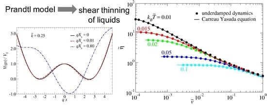
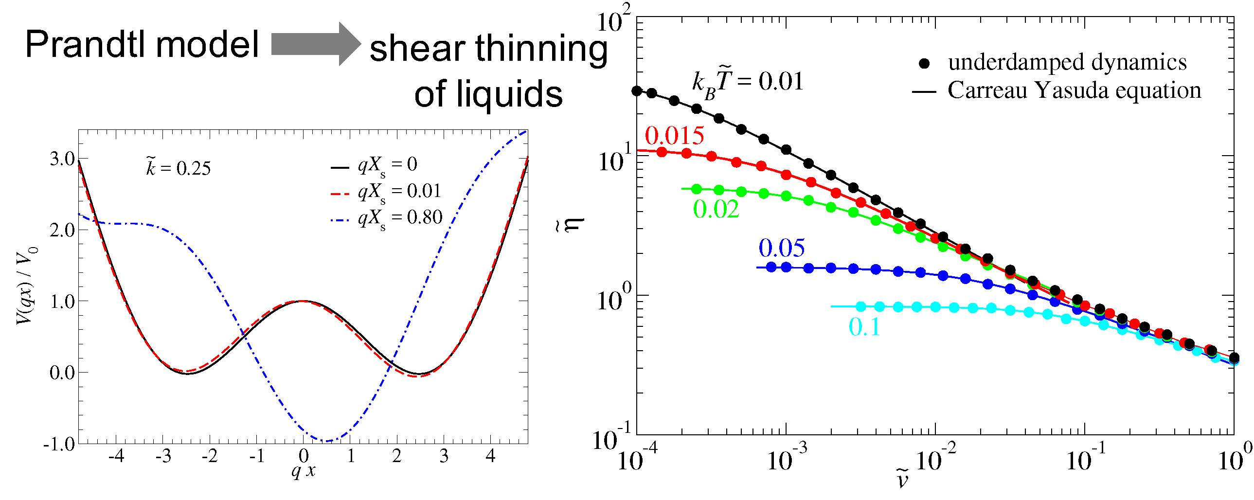
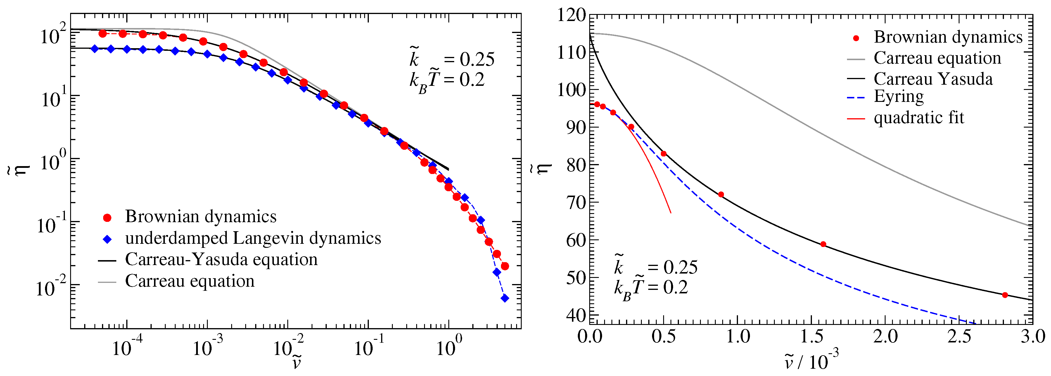
Figure 3 compares over- and underdamped dynamics for $\tilde{k}=0.25$ at a thermal energy of $k_B\tilde{T}=0.2$. Both curves show similar trends since they can both be fit very well over an extended velocity range with the CY equation. However, overdamped and underdamped $\tilde{\eta }\left(\tilde{v}\right)$ relations differ noticeably, in particular at very large and very small sliding velocities. Most importantly, the friction in the (slightly) underdamped case is reduced by a factor of approximately two in the $\tilde{v}\to 0$ limit.

The adjustable parameters of the CY equation were fit to the data presented in Figure 3 within the range ${10}^{-3}\le \tilde{v}\le 0.1$. Results for the fits are stated in the figure caption. The two dimensionless exponents n and a happen to be reasonably close to those reported by Yasuda for polystyrene [21,22]. Significant similarity between our results and Yasuda’s data on polystyrene is certainly also revealed by eye when comparing our Figure 3 to Figure 4.1-3 in Ref. [22]. We are certain that the agreement can be further significantly improved by slightly increasing $\tilde{k}$ and reducing $\tilde{m}$, and, most importantly, by introducing a Stokesian damping between the mass point and the moving external potential. The last modification of our model would make the damping/viscosity level off at a finite value for large shear rates.

A large-velocity regime can be identified, in which the CY equation reflects the data extremely well when plotted in double logarithmic fashion. However, it does not accurately describe the changes of the effective damping at very small sliding velocities, as can be seen from the right graph in Figure 3. For $\tilde{v}\lesssim {\tilde{v}}_0/3$, the effective damping obeys a quadratic $\tilde{v}$ dependence, as expected from perturbation theory. Both the Eyring model and an even-power, second-order Taylor series expansion of the effective damping into $\tilde{\eta }\approx {\tilde{\eta }}_0+{\tilde{\eta }}^{″}\left(0\right){\dot{\gamma }}^2/2$ accurately reflect the low-velocity regime. The range in which Eyring is a reasonable approximation to the true data is certainly much larger than for a second-order Taylor series expansion. However, corrections to Eyring remain necessary to reach satisfactory agreement to values of $\tilde{v}$ beyond ${\tilde{v}}_0$, e.g., in terms of a shear-rate or shear-stress dependent activation barrier.

Despite the close agreement between the simulation data and the CY equation at intermediate velocities, it must be noted that the agreement is not perfect. Systematic and non-monotonic deviations of order 5% occur, i.e., a quasi-exact proportionality between damping and velocity ($\tilde{F}\propto {\tilde{v}}^n$) at intermediate velocities, is not produced by the Prandtl model. We expect the same to hold for real, high-precision viscosity measurements as well.

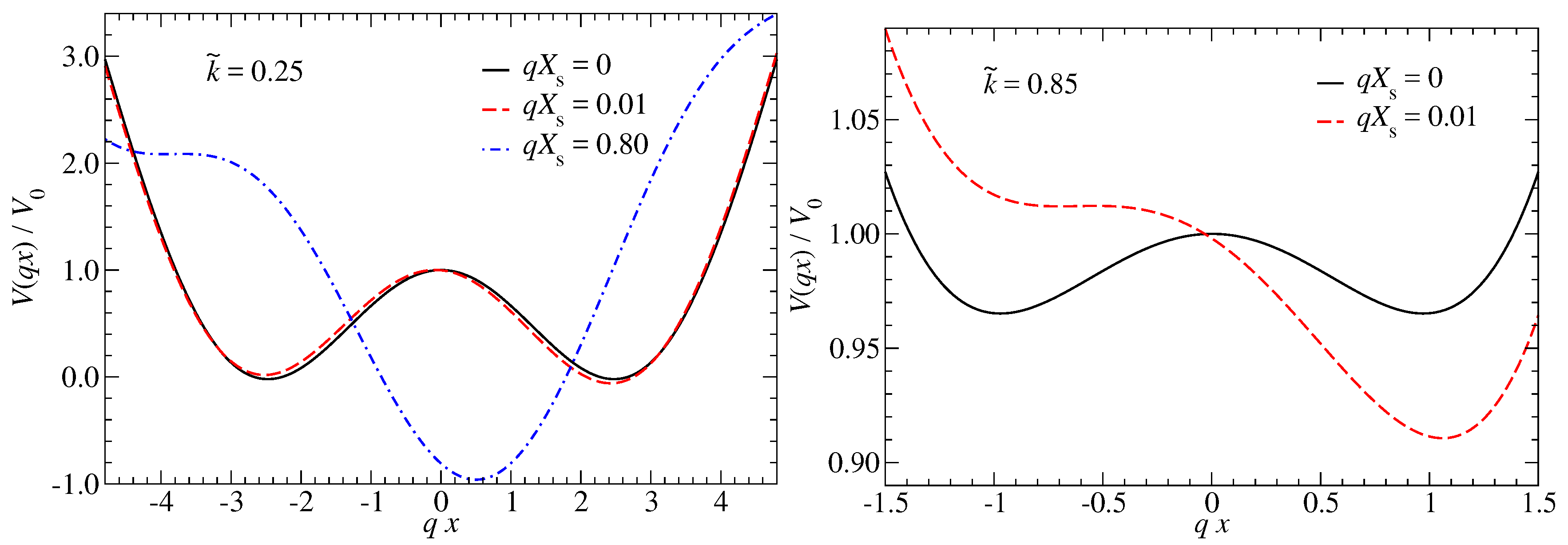
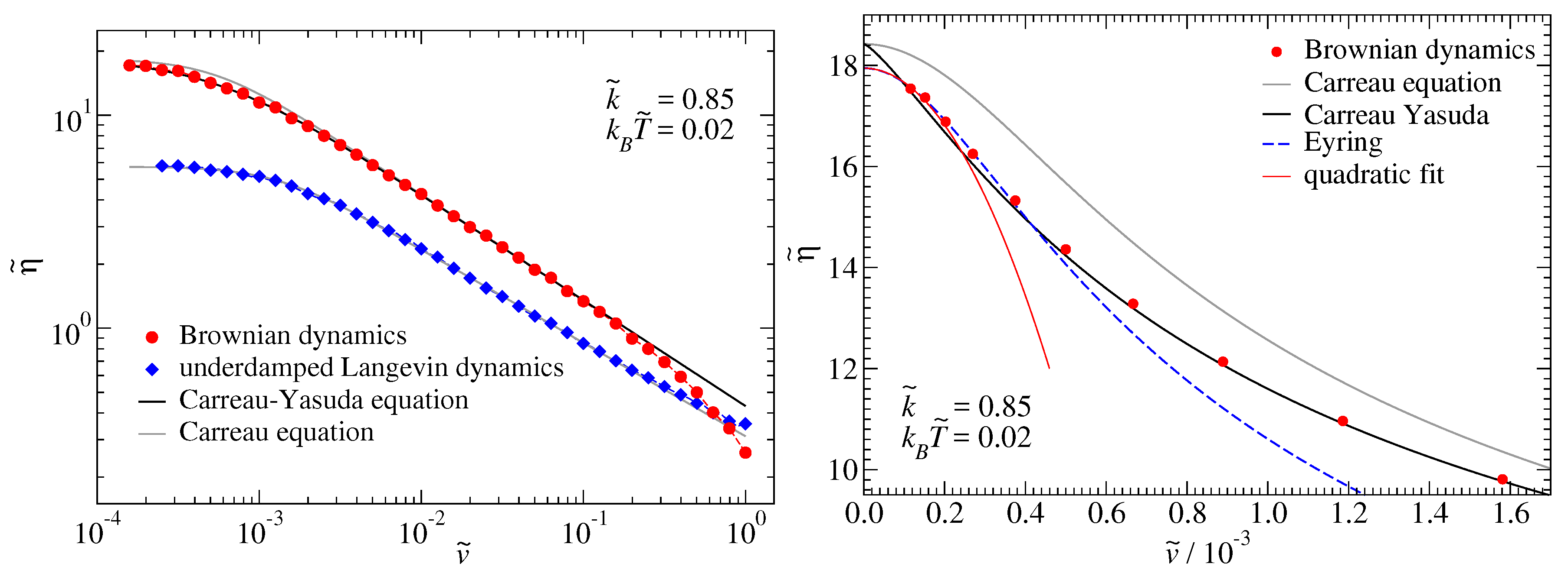
When $\tilde{k}$ is increased, the friction–velocity relation continues to be described quite well by the CY relation, as can be seen in Figure 4 for $\tilde{k}=0.85$. The exponent n is noticeably reduced compared to that obtained for the more compliant $\tilde{k}=0.25$ spring, specifically it acquires a value close to 0.5, which is representative of human blood [28]. To what extent this agreement is coincidental is discussed in Section 4.

While the rheological responses shown in Figure 3 and Figure 4 are quite similar, some differences appear to be worth noting. First, the discrepancy between over- and underdamped friction has become more significant at the larger value of $\tilde{k}$: it grew from a factor of two to a factor of three. Second, at the smaller reduced spring stiffness, both rheological response functions clearly required the exponent a to be less than 2. For the larger reduced spring stiffness, the rheological response function of the underdamped system could be very well described with $a=2$, i.e., the value that a takes in the Carreau model, while an accurate description of the overdamped system necessitated a value close to unity. Third, the low-$\tilde{v}$ expansions (Taylor or Eyring) of the effective damping always remained smaller than the fit to the CY equation in case of the small value of $\tilde{k}$, but not for the larger value.

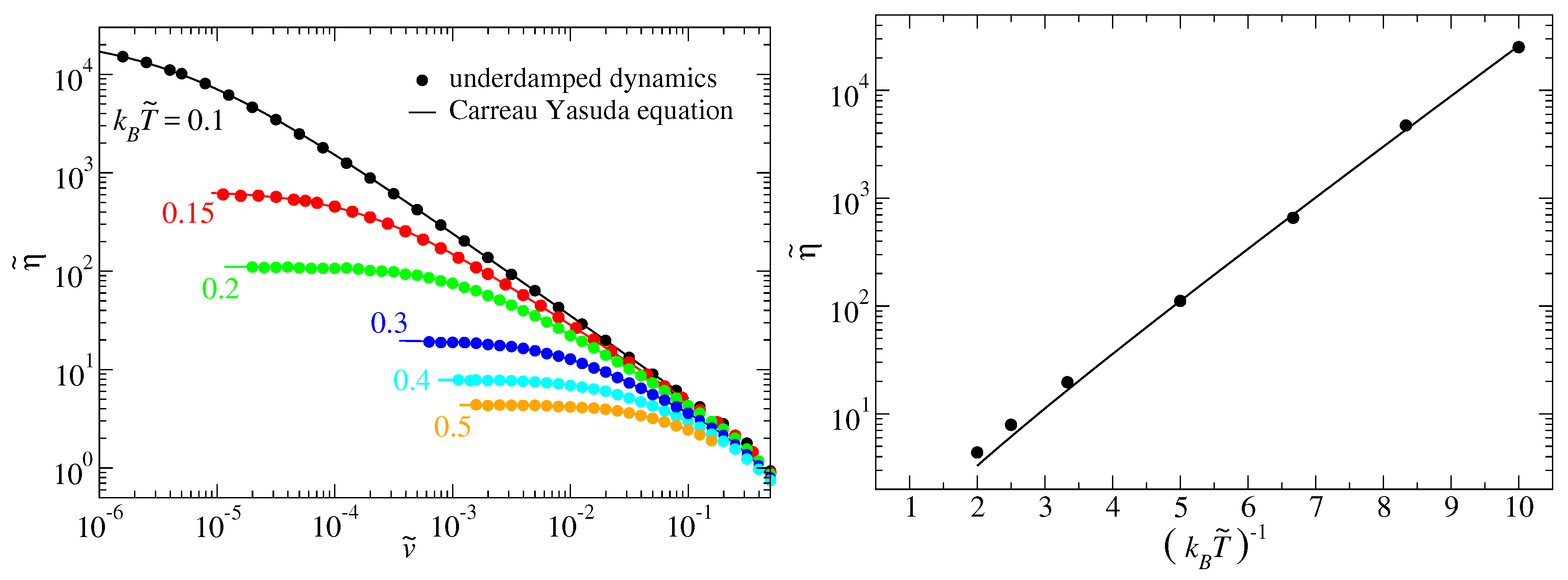
We next investigate how the $\tilde{\eta }\left(\tilde{v}\right)$ relation depends on temperature for the two reduced spring stiffnesses investigated so far. The left graph in Figure 5 shows data for $\tilde{k}=0.25$ and reveals the following, frequently observed behavior: The temperature dependence of damping is less pronounced at high than at low shear rates and the transition between non-Newtonian and Newtonian behavior moves to smaller velocities at decreasing temperature. Coefficients deduced from fits to the Carreau–Yasuda equation read for the two most extreme investigated temperatures are: $\tilde{\eta }$ = 25,200, $\tilde{v}=4.20\times {10}^{-6}$, $a=0.685$, and $n=0.156$ for $k_B\tilde{T}=0.1$ and $\tilde{\eta }=4.38$, $\tilde{v}=4.13\times {10}^{-2}$, $a=1.51$, and $n=0.436$ for $k_B\tilde{T}=0.5$. Thus, damping increases by roughly four orders of magnitude upon cooling as the thermal energy is decreased from $k_B\tilde{T}=0.5$ to $k_B\tilde{T}=0.1$, while the cross-over velocity decreases by a similar factor. In addition, the exponent n decreases upon cooling, while a increases. In fact, $n(k_B\tilde{T}=0.1)$ is so close to zero that the resulting power law $F\propto v^n$ is difficult to distinguish from a logarithmic dependence in a double logarithmic representation unless v spans more than two decades.

Similar to the exponent n, the exponent a decreases systematically with decreasing temperature, When the thermal energy is no longer very small compared to $\Delta E\approx 0.0348$, it appears that data can be described by assuming $a=2$, as revealed for $k_B\tilde{T}=0.02$. However, while data appear to be perfectly consistent with the Carreau equation, as can be seen in Figure 5, the fit further improves by setting a to $a=1.57$.

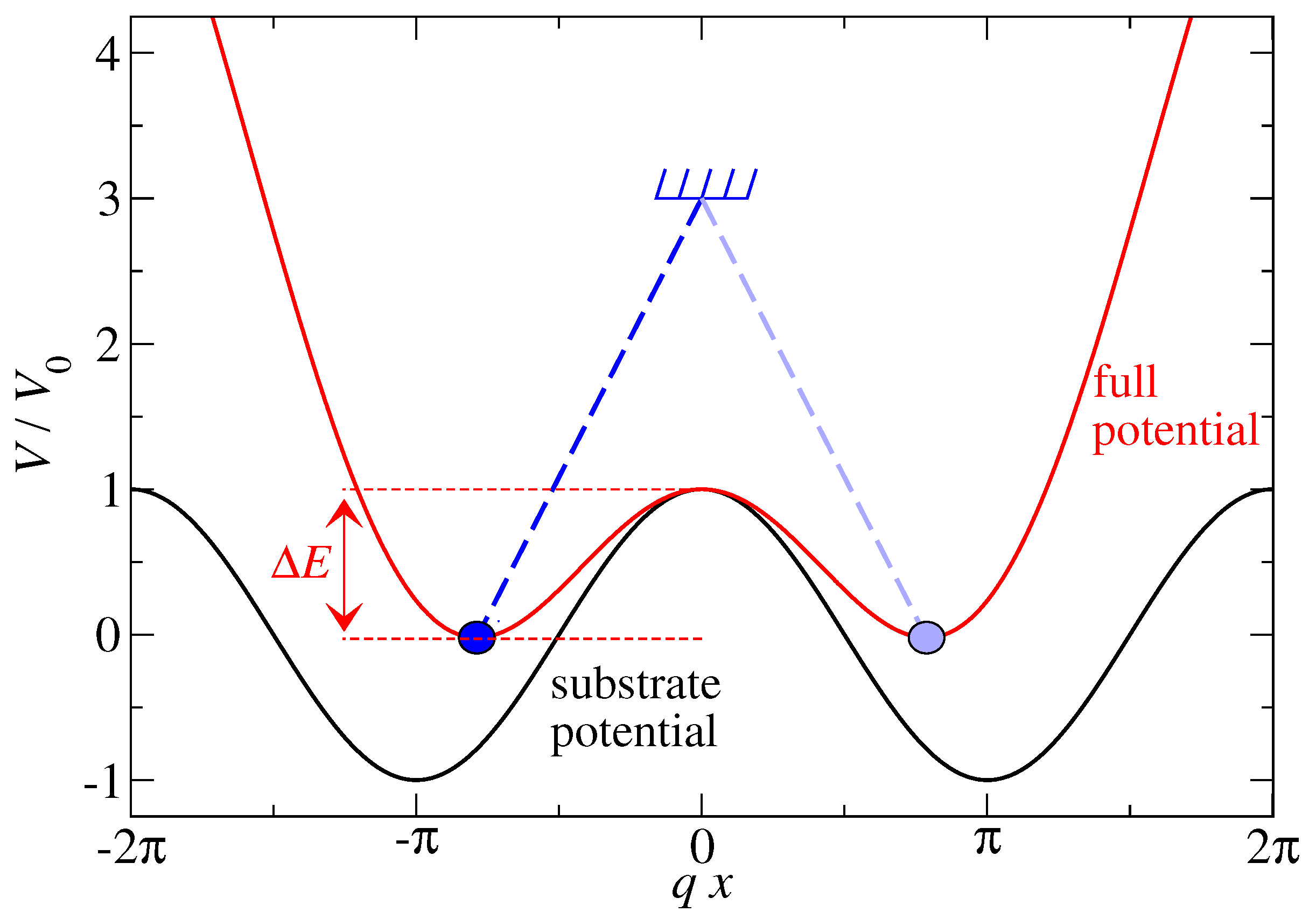
The temperature dependence of the effective damping is analyzed in the right graph of Figure 5. At low temperatures, it satisfies Equation (6), where $\Delta \tilde{E}=1.02023$ was determined, as indicated in Figure 1. Thus, only $k_B{\tilde{T}}_{\eta }=10.9$ and ${\alpha }_{\eta }=0.5$, were adjusted for Equation (6) to fit the simulated data.

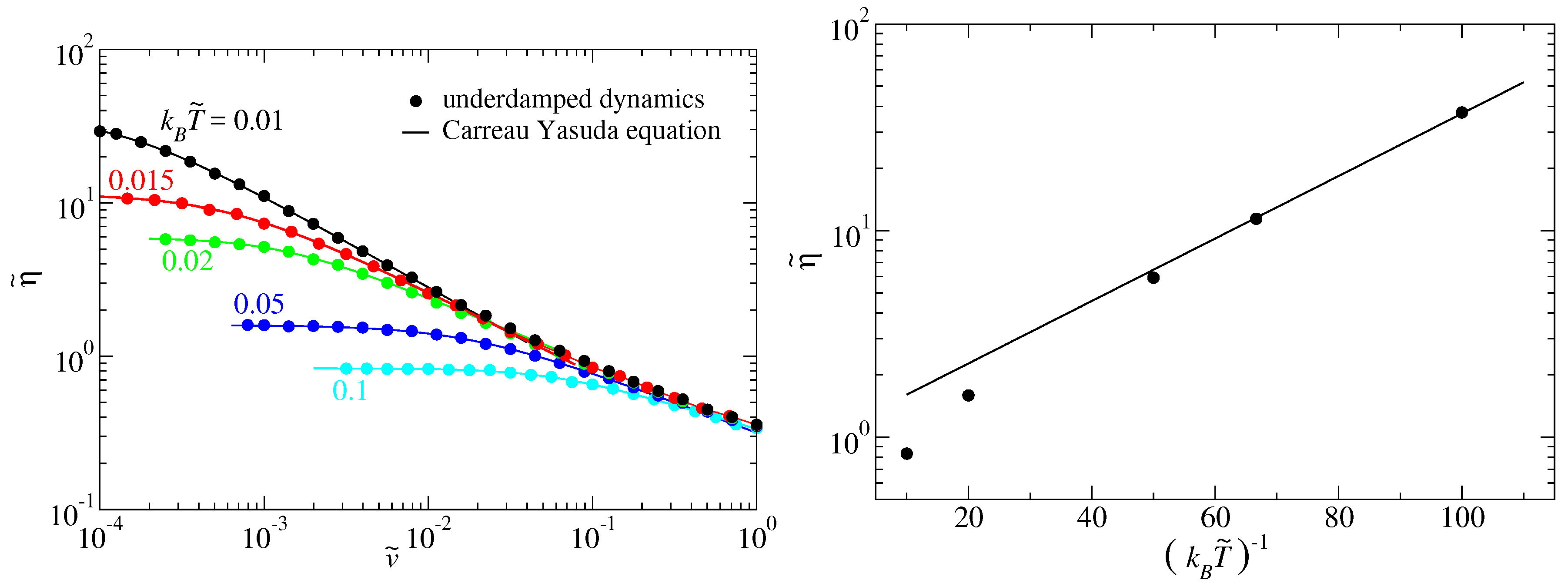
The just reported analysis was repeated for $\tilde{k}=0.85$ and the pertinent results presented in Figure 6. For the softer springs, $\Delta \tilde{E}$ is reduced to approximately 0.035, which in turn is consistent with a reduction of the exponent n. The exponential increase of damping at small thermal energies with inverse temperature can again be described assuming the barrier depicted in Figure 1 to be the relevant one. However, the prefactor to $\tilde{\eta }$ at small $k_B\tilde{T}$ is now consistent with an essentially constant value near unity. To ascertain if the indicated low-temperature behavior is truly asymptotic for either $\tilde{k}=0.25$ or $\tilde{k}=0.85$, a lower temperature would have to be reached. We plan on addressing this in the future either using improved integration schemes for the FPE or a pertubative treatment.

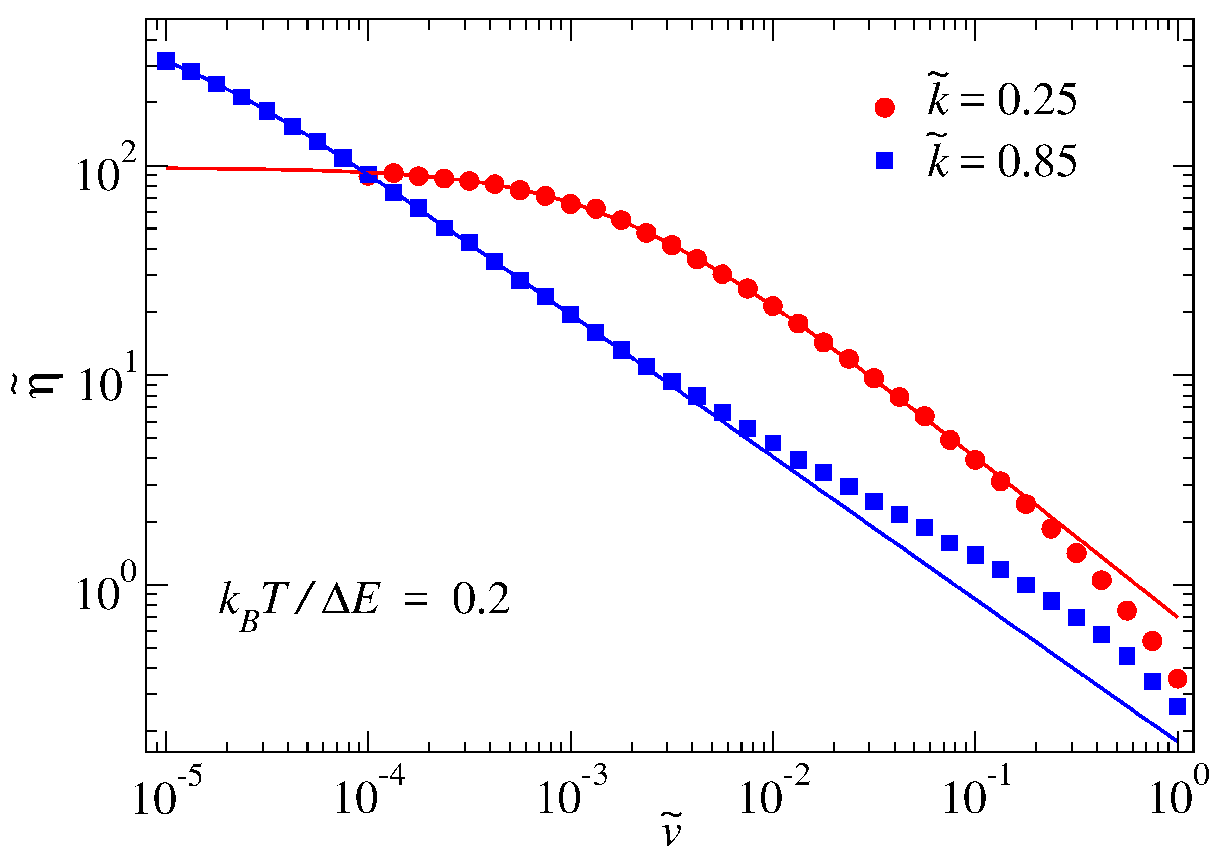
The next simulation data presented explicitly is meant to test the order-of-magnitude estimates of the equilibrium damping made in Section 2.1.2. Towards this end, the velocity dependence of the damping term is computed for the two spring stiffnesses $\tilde{k}=0.25$ and $\tilde{k}=0.85$ at a fixed value of $k_{B}T/\Delta E=0.2$. Results are presented in Figure 7. The dominant factor $exp(\Delta E/k_{B}T)$ in Equation (6) yields $\approx 150$, which is 1.5 larger than the value for $\tilde{k}=0.25$ reported in the caption of Figure 7 and a little less than a third predicted for $\tilde{k}=0.85$. The cross-over velocities were crudely estimated to differ by a factor of 80 in the discussion of Figure 2. This is to be compared to a ratio of 190 found in the full simulations. Thus, additional work is required to develop better estimates.

An interesting trend revealed in Figure 7 relates to the breakdown of the Carreau–Yasuda equation at large velocities. It can either overestimate or underestimate the true damping when parameters were fitted to the cross-over region and predictions then made for large shear rates. Since the high-temperature viscosity ${\eta }_{\infty }$ is usually a fit parameter (while it was set and thus known to disappear in the current study), the regime for which CY is believed to be valid for given experimental data can be easily overestimated. In any event, the appearance of a shoulder at large velocities and values of $\tilde{k}$ approaching unity from below is observed for both underdamped as well as overdamped dynamics.

In the data shown explicitly in this work thus far, the values for the two dimensionless exponents in the CY equation range from 0.156 to 0.769 for n and from 0.685 to 1.66 for a. Many additional simulations were run outside this range, which corroborated the expectation that n can take any value in between zero (for $\tilde{k}\to 0$) and unity (for $\tilde{k}\to 1$). This expectation arises from the observation that the Prandtl model reduces to Eyring in the $\tilde{k}\to 0$ limit so that $n\to 0$ follows automatically, while, for $\tilde{k}>1$, the friction for the Prandtl model is Stokesian at small velocities, even without thermal fluctuations.

The final systematic analysis is concerned with the analysis of how the effective free-energy barrier, defined in Equation (3), depends on the shear stress. Results for $\tilde{k}=0.02$ (overdamped dynamics) and $\tilde{k}=0.25$ (underdamped dynamics) are shown in Figure 8.

The data for $\tilde{k}=0.02$ reveals an astonishingly good agreement between simulation and the theory developed in Section 2.1.3 for the force-induced reduction of the effective free-energy barrier. These corrections are a function of the shape of the corrugation potential. They would therefore be different if the corrugation potential had a different functional dependence by including higher-order harmonics. The original Eyring theory, which does not include shear-force induced corrections to the free-energy barrier, provides an upper bound for the reduction $\Delta F$, which is approached from below as T is decreased. The data for $\tilde{k}=0.02$ consolidates the claim that the Eyring model is obtained as a limiting case of the Prandtl model, even if $\tilde{k}=0.02$ is still not fully $\tilde{k}=0^{+}$.

The effect of shear stress on the reduction of the effective energy-barrier is qualitatively similar for $\tilde{k}=0.25$ as for the just-discussed $\tilde{k}=0.02$. The reduction is again roughly linear in the (shear) force and only crosses over to a parabolic-like dependence at very small values of $\tilde{v}$. The change of the energy-barrier reduction (as measured in units of $k_{B}T$) with $\tilde{f}/\left(k_B\tilde{T}\right)$ is similar in magnitude for both $\tilde{k}$; however, it is slightly reduced for the larger $\tilde{k}$. The reduction of this slope is much more significant for $\tilde{k}=0.85$, which is not shown explicitly. In all cases, the slope in the linear regime can be very roughly approximated to be $q\Delta x_{\mathrm{B}}/\pi$, where $\Delta x_{\mathrm{B}}$ is the distance between the location of the minimum and that of the barrier in the force-free case.

Outside the range of instabilities ($\tilde{k}>1$), the Prandtl model predicts shear thickening at small $\tilde{v}$. The corresponding data, which is not shown explicitly, is again consistent with the CY equation over two or three decades in shear rate. In the Prandtl model, this shear thickening could be the consequence of resonance effects that arise because the substrate potential reaches the spring’s eigenfrequency, or, in the case of overdamping, the inverse relaxation time. Thus, in an atomistic interpretation of the Prandtl model, velocities near the speed of sound would be required to approach those frequencies. Consequently, strong non-linearities, such as heating, cavitation, chemical break-down of the lubricant, etc. would arise, which are all not captured by the model. This is why it would be meaningless to study resonance in this case. However, if the mass point of the Prandtl model represented a coarse-grained degree of freedom, resonance effects are possible at velocities much below the speed of sound.

4. Discussion and Conclusions

In this work, the rheology associated with the Prandtl model was studied and found to be very similar to the rheology of real liquids. In particular, by converting the velocity dependence of damping to a shear-rate dependence of the effective viscosity, the rheological response of the Prandtl model reproduced the Carreau–Yasuda equation over a large range. A similarly satisfactory description could not be achieved with other phenomenological descriptions over the same range using only the same number of adjustable parameters. The crude interpretation of shear thinning in the Prandtl model is similar to the one described by Lacks [29] for a more realistic, all-atom model, consisting of binary, glass-forming Lennard–Jonesium: The viscosity can be [is] separated into a “structural” contribution associated with the energy minima that the system visits, and a “vibrational” contribution associated with displacements within the energy minima. The structural contribution is shear thinning due to strain-activated relaxations caused by the disappearance of high-stress energy minima, while the vibrational contribution is Newtonian. This sudden disappearance of high-stress energy minima does not occur in the Eyring ($\tilde{k}\to 0$) limit of the Prandtl model, but only for finite values below the critical stiffness, i.e., it necessitates the elastic component of a fluid’s viscoelastic properties.

Due to its simplicity, the Prandtl model allows some fundamental questions to be investigated with a high (numerical) precision, which might not be achievable experimentally, or when conducting simulations of more explicit and realistic models, although such simulations have now reached an impressive accuracy [17,19,30]. This concerns in particular the analysis of the initial stages of shear thinning at extremely small shear rates. We found that leading-order corrections to the effective Newtonian viscosity are quadratic in velocity (and thus quadratic in friction or shear stress), but that this initial regime can be extremely narrow. At the same time, the effect of this initial transition to the cross-over regime (i.e., when sliding velocities are of a similar order of magnitude as the parameter $v_0$ in the CY equation) can still be significant, even if the CY equation appears to be a perfect fit. In the Prandtl model, equilibrium damping can be easily overestimated by as much as 20%, by extrapolating the damping from $v=v_0$ to $v=0$ using the CY equation. As such, we suggest that Newtonian viscosities should generally lie between the apparent viscosity measured at the smallest shear rate and the value obtained from fits to phenomenological equations such as Carreau–Yasuda, at least as long as the experimental data extend only to the cross-over shear rate.

Interestingly, the Prandtl model yields a broad range of values of the exponent n in the CY equation, depending on the temperature and velocity; any value $0<n<1$ appears to be possible. Lowering the reduced temperature and/or decreasing the dimensionless spring constant lowers n. For $\tilde{k}>1$, shear thickening can be obtained. A single dissipative spring suffices to accomplish this, even if the model can be readily generalized to yield more complex rheology by augmenting or replacing the spring with other rheological elements composed of springs and dashpots, such as those defining Maxwell and Kelvin–Voigt materials. Particularly meaningful would be to introduce an additional damping element in series with the current dissipative spring, in which the time constant of the new damping element reflects the life time of the local topology or “cage” into which an individual atom is embedded. The topology can be defined by quenching a fluid via a steepest descent to the nearest minimum [31]. Once properly parameterized, such (thermostatted) Prandtl models show great potential for modeling complex rheological responses of liquids for which the use of many conventional rheological elements is currently needed when their relaxation functions cover several decades in time.

The numerical studies presented in this work were focused on two particular values of $\tilde{k}$. For $\tilde{k}=0.25$ and intermediate values of $\tilde{T}$, the exponent n took values in the vicinity of 0.2, which is characteristic for many polymers under ambient conditions. For $\tilde{k}=0.85$, values near $n=1/2$ were obtained, which is close to that observed for human blood [28]. This in itself is not yet necessarily meaningful, but an interesting question is if the model allows the way in which the exponent n changes for different system to be rationalized.

For example, let us assume the Prandtl model is parameterized to reproduce the rheological response of a polymer under ambient conditions. As the temperature is lowered, the effective damping will increase at a given velocity, while the crossover velocity decreases substantially. This happens in such a way that the exponent n decreases in the Prandtl model upon cooling, as in a real liquid. When keeping the parameters in the Prandtl model fixed, this decrease is approximately exponential in inverse temperature, which would reflect the behavior of many liquids including glass-forming liquids cooled below their fragile-to-strong-transition temperature [32]. If the pressure were increased, the steric repulsion between non-bonded monomers would be enhanced so that an increased value of $V_0$ would have to be used in the Prandtl model to account for that increase. At the same time, the elasticity of individual polymers would scarcely change. Consequently, the dimensionless parameter n would be reduced along with $\tilde{k}$. This argument agrees with the known phenomenology of polymers.

Assume next that the Prandtl model is parameterized to reproduce the rheological response of human blood cells, for which $n=0.5$ appears to describe the shear thinning reasonably well [28]. Now, a camel comes along, which happens to belong to a species with extraordinarily stiff red blood cells [33]. It appears obvious that stiff springs have to be used in the Prandtl model to account for the stiff red blood cells of camels. Increasing the (dimensionless) stiffness in the Prandtl model significantly reduces shear thinning, in agreement with the rheology of camel blood [33]. There might be even more details of the rheological response of blood that the Prandtl model is able to reproduce. For example, at large velocities, the effective damping for $\tilde{k}=0.85$ does not quickly converge to the high-velocity limit, but shows an indication of a shoulder. A similar shoulder is also observed in detailed simulations of human blood cells as can be seen in Figure 1 of Ref. [34]. It is not clear at this point to what extent this similarity can be further increased with minor adjustments to the model or to what extent the shoulder in our simulations simply indicates a resonance of the spring at a given beat frequency. However, it is possible that the qualitative resemblance is not entirely coincidental. To demonstrate that this is indeed the case, a true bottom-up parameterization would be required, which is certainly beyond the scope of this work.

We conclude by quoting again Prandtl: “we obtain the complete transition from solid bodies to liquids of low viscosity including all states of softening in between”. While in today’s jargon one might talk about shear thinning rather than softening, our work reveals that Prandtl’s expectations were not too high. To reproduce the frequently observed characteristic power-law dependence of shear stress or effective viscosity on load, there is no need to postulate a (broad) distribution of energy barriers as done by Ree and Eyring [35]. Prandtl’s model can be parameterized to represent not only the temperature and velocity dependence measured in atomic-force microscopy experiments but also the shear thinning of fluids as diverse and complex as polystyrene and blood.

References

1. Prandtl, L. Ein Gedankenmodell zur kinetischen Theorie der festen Körper. Z. Angew. Math. Mech. 1928, 8, 85–106. [Google Scholar] [CrossRef]
2. Müser, M.H.; Urbakh, M.; Robbins, M.O. Statistical Mechanics of Static and Low-Velocity Kinetic Friction. In Advances in Chemical Physics; John Wiley & Sons, Inc.: Hoboken, NJ, USA, 2003; pp. 187–272. [Google Scholar] [CrossRef]
3. Popov, V.; Gray, J. Prandtl-Tomlinson model: History and applications in friction, plasticity, and nanotechnologies. ZAMM J. Appl. Math. Mech. 2012, 92, 683–708. [Google Scholar] [CrossRef]
4. Coulomb, C.A. Théorie des machines simples. Mem. Math. Phys. l’Acadmie R. 1785, 161–342. [Google Scholar]
5. Gnecco, E.; Bennewitz, R.; Gyalog, T.; Loppacher, C.; Bammerlin, M.; Meyer, E.; Güntherodt, H.J. Velocity Dependence of Atomic Friction. Phys. Rev. Lett. 2000, 84, 1172–1175. [Google Scholar] [CrossRef] [PubMed]
6. Maier, S.; Sang, Y.; Filleter, T.; Grant, M.; Bennewitz, R.; Gnecco, E.; Meyer, E. Fluctuations and jump dynamics in atomic friction experiments. Phys. Rev. B 2005, 72, 245418. [Google Scholar] [CrossRef] [Green Version]
7. Fusco, C.; Fasolino, A. Velocity dependence of atomic-scale friction: A comparative study of the one- and two-dimensional Tomlinson model. Phys. Rev. B 2005, 71. [Google Scholar] [CrossRef] [Green Version]
8. Krylov, S.Y.; Frenken, J.W.M. The crucial role of temperature in atomic scale friction. J. Phys. Condens. Matter 2008, 20, 354003. [Google Scholar] [CrossRef]
9. Hölscher, H.; Schirmeisen, A.; Schwarz, U.D. Principles of atomic friction: From sticking atoms to superlubric sliding. Philos. Trans. R. Soc. A Math. Phys. Eng. Sci. 2008, 366, 1383–1404. [Google Scholar] [CrossRef]
10. Szlufarska, I.; Chandross, M.; Carpick, R.W. Recent advances in single-asperity nanotribology. J. Phys. D Appl. Phys. 2008, 41, 123001. [Google Scholar] [CrossRef] [Green Version]
11. Socoliuc, A.; Bennewitz, R.; Gnecco, E.; Meyer, E. Transition from Stick-Slip to Continuous Sliding in Atomic Friction: Entering a New Regime of Ultralow Friction. Phys. Rev. Lett. 2004, 92, 134301. [Google Scholar] [CrossRef]
12. Müser, M.H. Structural lubricity: Role of dimension and symmetry. Europhys. Lett. EPL 2004, 66, 97–103. [Google Scholar] [CrossRef]
13. Müser, M.H. Velocity dependence of kinetic friction in the Prandtl-Tomlinson model. Phys. Rev. B 2011, 84, 125419. [Google Scholar] [CrossRef] [Green Version]
14. Spikes, H.; Tysoe, W. On the Commonality Between Theoretical Models for Fluid and Solid Friction, Wear and Tribochemistry. Tribol. Lett. 2015, 59. [Google Scholar] [CrossRef]
15. Evans, C.R.; Johnson, K.L. The Rheological Properties of Elastohydrodynamic Lubricants. Proc. Inst. Mech. Eng. Part C J. Mech. Eng. Sci. 1986, 200, 303–312. [Google Scholar] [CrossRef]
16. Dench, J.; di Mare, L.; Morgan, N.; Wong, J.S.S. Comparing the molecular and global rheology of a fluid under high pressures. Phys. Chem. Chem. Phys. 2018, 20, 30267–30280. [Google Scholar] [CrossRef] [PubMed]
17. Galvani Cunha, M.A.; Robbins, M.O. Determination of pressure-viscosity relation of 2, 2, 4-trimethylhexane by all-atom molecular dynamics simulations. Fluid Phase Equilibria 2019, 495, 28–32. [Google Scholar] [CrossRef] [Green Version]
18. Eyring, H. Viscosity, Plasticity, and Diffusion as Examples of Absolute Reaction Rates. J. Chem. Phys. 1936, 4, 283–291. [Google Scholar] [CrossRef]
19. Jadhao, V.; Robbins, M.O. Rheological Properties of Liquids Under Conditions of Elastohydrodynamic Lubrication. Tribol. Lett. 2019, 67. [Google Scholar] [CrossRef] [Green Version]
20. Carreau, P.J. Rheological Equations from Molecular Network Theories. Trans. Soc. Rheol. 1972, 16, 99–127. [Google Scholar] [CrossRef]
21. Yasuda, K. Investigation of the Analogies between Viscometric and Linear Viscoelastic Properties of Polystyrene Fluids. Ph.D. Thesis, Massachusetts Institute of Technology, Cambridge, MA, USA, 1979. [Google Scholar]
22. Bird, R.B.; Armstrong, R.C.; Hassager, O. Dynamics of Polymeric Fluids. Volume 1: Fluid Mechanics; John Wiley & Sons: New York, NY, USA, 1987. [Google Scholar]
23. Zhang, J.; Spikes, H. On the Mechanism of ZDDP Antiwear Film Formation. Tribol. Lett. 2016, 63. [Google Scholar] [CrossRef] [Green Version]
24. Sang, Y.; Dubé, M.; Grant, M. Thermal Effects on Atomic Friction. Phys. Rev. Lett. 2001, 87, 174301. [Google Scholar] [CrossRef] [PubMed] [Green Version]
25. Dudko, O.; Filippov, A.; Klafter, J.; Urbakh, M. Dynamic force spectroscopy: A Fokker–Planck approach. Chem. Phys. Lett. 2002, 352, 499–504. [Google Scholar] [CrossRef]
26. Adelman, S.A.; Doll, J.D. Generalized Langevin equation approach for atom/solid-surface scattering: General formulation for classical scattering off harmonic solids. J. Chem. Phys. 1976, 64, 2375. [Google Scholar] [CrossRef]
27. Risken, H. The Fokker-Planck Equation; Springer: Berlin, Germany, 1989. [Google Scholar]
28. Cho, Y.I.; Cho, D.J. Hemorheology and Microvascular Disorders. Korean Circ. J. 2011, 41, 287. [Google Scholar] [CrossRef] [Green Version]
29. Lacks, D.J. Energy Landscapes and the Non-Newtonian Viscosity of Liquids and Glasses. Phys. Rev. Lett. 2001, 87, 225502. [Google Scholar] [CrossRef]
30. Cui, S.T.; Gupta, S.A.; Cummings, P.T.; Cochran, H.D. Molecular dynamics simulations of the rheology of normal decane, hexadecane, and tetracosane. J. Chem. Phys. 1996, 105, 1214–1220. [Google Scholar] [CrossRef] [Green Version]
31. Stillinger, F.H.; Weber, T.A. Hidden structure in liquids. Phys. Rev. A 1982, 25, 978–989. [Google Scholar] [CrossRef]
32. Angell, C. Relaxation in liquids, polymers and plastic crystals—Strong/fragile patterns and problems. J. Non-Cryst. Solids 1991, 131–133, 13–31. [Google Scholar] [CrossRef]
33. Windberger, U.; Auer, R.; Seltenhammer, M.; Mach, G.; Skidmore, J.A. Near-Newtonian Blood Behavior—Is It Good to Be a Camel? Front. Physiol. 2019, 10. [Google Scholar] [CrossRef] [Green Version]
34. Fedosov, D.A.; Pan, W.; Caswell, B.; Gompper, G.; Karniadakis, G.E. Predicting human blood viscosity in silico. Proc. Natl. Acad. Sci. USA 2011, 108, 11772–11777. [Google Scholar] [CrossRef] [Green Version]
35. Ree, T.; Eyring, H. Theory of Non-Newtonian Flow. I. Solid Plastic System. J. Appl. Phys. 1955, 26, 793–800. [Google Scholar] [CrossRef]
Figure 1. Energy landscape of the Prandtl model for k ˜ = 0.25 at a point of time, when both energy minima are equivalent. Δ E indicates the energy barrier separating the motion of the atom from one minimum to the next.
Lubricants 08 00038 g001
Figure 2. Full potential energy landscape of the Prandtl model for (left) k ˜ = 0.25 and (right) k ˜ = 0.85 at different relative displacements between substrate and spring.
Lubricants 08 00038 g002
Figure 3. Effective damping η ˜ as a function of velocity v ˜ for k ˜ = 0.25 and k B T ˜ = 0.2 . (Left) Comparison of overdamped (red circles) and underdamped (blue diamonds) dynamics, the latter being based on a reduced mass of m ˜ = 1 / 4 . The black lines are fits to the CY equation. Both fits were done in the interval 3 × 10 4 v ˜ 0.1 but plotted over a larger velocity range. Values for the Carreau–Yasuda fits are: γ ˜ = 115 , v ˜ 0 = 1.63 × 10 3 , n = 0.196 , and a = 0.812 for the overdamped system and γ ˜ = 56.7 , v ˜ 0 = 2.41 × 10 3 , n = 0.268 , and a = 1.05 in the underdamped case. The Carreau equation is parameterized as CY, however, with a = 2 . (Right) Analysis of the small-velocity damping. The Carreau and CY models were left unchanged with respect to the left figure. Additional models include the Eyring model η ˜ = η ˜ 0 v ˜ 0 arsinh ( v ˜ / v ˜ 0 ) and a quadratic approximation, η ˜ = η ˜ 0 + η ˜ 0 v ˜ 2 / 2 , for which the parameters ( η ˜ 0 , v ˜ 0 and η ˜ ) were adjusted to the asymptotic v ˜ 0 dependence of η ˜ .
Lubricants 08 00038 g003
Figure 4. Similar to Figure 3, but for k ˜ = 0.85 and k B T ˜ = 0.02 . Parameters used in the Carreau–Yasuda equation are this time γ ˜ = 18.4 , v ˜ 0 = 0.522 × 10 3 , n = 0.503 , and a = 1.28 for the overdamped system and γ ˜ = 5.73 , v ˜ 0 = 1.30 × 10 3 , n = 0.521 , and a = 2 in the underdamped case.
Lubricants 08 00038 g004
Figure 5. (Left) η ˜ ( v ˜ ) dependence in the underdamped Prandtl model for k ˜ = 0.25 at various temperatures. Symbols show data from MD simulations, while lines are fits to the Carreau–Yasuda equation. The most extreme values for n and a turned out to be n = 0.156 , a = 0.685 at k B T ˜ = 0.1 and n = 0.371 , a = 1.33 at k B T ˜ = 0.5 . (Right) Reduced Newtonian damping η ˜ as a function of inverse reduced temperature ( k B T ˜ ) 1 . Circles show results from fits of the MD data to the Carreau–Yasuda equation. The solid line is a low-temperature fit of the data to Equation (6), where Δ E ˜ ( k ˜ = 0.25 ) = 1.02023 is determined as described in Figure 1 with an exponent α η = 1 / 2 .
Lubricants 08 00038 g005
Figure 6. Same as Figure 5, but this time for k ˜ = 0.85 , for which Δ E ( k ˜ = 0.85 ) = 0.0348182 . The solid line obeys Equation (6), however, the temperature-dependent prefactor is replaced with the constant 1.13. The most extreme values for n and a in the left graph were n = 0.403 , a = 1.34 at k B T ˜ = 0.01 and n = 0.668 , a = 1.66 at k B T ˜ = 0.1 .
Lubricants 08 00038 g006
Figure 7. Effective damping η ˜ for overdamped dynamics as a function of sliding velocity v ˜ for two different stiffnesses at a constant ratio of k B T / Δ E = 0.2 . The low-velocity η ˜ ( v ˜ ) dependence is consistent with the CY parameters η N = 97.8 , v 0 = 1.62 × 10 3 , n = 0.769 , and a = 0.97 for k ˜ = 0.25 and η N = 498 , v 0 = 8.52 × 10 6 , n = 0.680 , and a = 1.16 for k ˜ = 0.85 .
Lubricants 08 00038 g007
Figure 8. Shear-thinning expressed via ln ( η N / η ) as a function of f ˜ / ( k B T ˜ ) . The term ln ( η N / η ) corresponds to the shear-force induced reduction of the free-energy barrier in units of k B T or Δ 2 F / ( k B T ) . Full symbols show data on the branch for which the friction force increases with sliding velocity, while open symbols relate to the remaining data. (Left) k ˜ = 0.02 and Brownian dynamics. Full lines show the theory as summarized in Equations (11) through (13). The dashed line shows an unmodified Eyring theory, which assumes f 0 to be constant, i.e., to be f 0 = q k B T / π . (Right) k ˜ = 0.25 and Langevin dynamics. The thin line is drawn to guide the eye.
Lubricants 08 00038 g008