Article

Friction Energy-Based Wear Simulation for Radial Shaft Sealing Ring

1
Institute of Machine Elements, Gears and Transmissions, University of Kaiserslautern, 67663 Kaiserslautern, Germany
2
Corporate Research and Development, Friedrichshafen AG, 88038 Friedrichshafen, Germany
*
Author to whom correspondence should be addressed.
Lubricants 2020, 8(2), 15; https://doi.org/10.3390/lubricants8020015
Submission received: 31 October 2019 / Revised: 20 January 2020 / Accepted: 1 February 2020 / Published: 4 February 2020
(This article belongs to the Special Issue Selected Papers from the 60th German Tribology Conference 2019)

Abstract

:
Radial shaft sealing rings (RSSR) are important machine elements used in rotating and oil lubricated systems. Their main task is to prevent oil from exiting the system and dirt particles from entering the system. When this function is not fulfilled, a leakage can occur and cause excessive damage after certain operating times, such as gear failure due to insufficient lubrication. This is the reason for the high level of current research interest in seals. The sealing function of RSSR occurs in the contact area between the sealing lip and the shaft. The contact takes place over a very small contact width of approximately 1 μm. These extremely small dimensions and the complex relationships between the functional influencing variables on the radial shaft sealing system make it difficult to simulate wear on the sealing ring. The energetic consideration of the wear process offers the possibility of quantifying influencing variables more easily by their energetic contribution, which can be determined experimentally. Based on experimentally measured total friction moments, and with the help of a semi-analytical (SA) solid contact model based on the half-space theory, this paper presents a modelling approach for the calculation of wear at the sealing ring. The model presented in this work differs from the existing models in two ways. The first particularity is the coupling of SA method with finite element method (FEM) for the resolution of the contact between the sealing lip and the shaft, allowing a fine discretization of the contact zone (by SA method) and the consideration of the structural behavior (by FE method). The SA method compared to the commonly used FEM presents a great saving in computation time. The second particularity is the use of the real data obtained during the wear tests. Most existing simulation models are based purely on contact pressure. This means that through the contact pressure obtained by simulation and a given sliding distance value, a friction energy will be estimated which will be used in a next step using a wear model such as Archad’s to calculate the wear rate. In this publication the value of friction energy was obtained directly on an experimental basis and a more appropriate wear law, such as Fleischer’s, taking into account the friction conditions, was used to estimate the wear rate.

Graphical Abstract

1. Introduction

This paper presents a SA method for wear prediction at the radial shaft sealing rings (RSSR) tribological system. The model presented in this work was validated by a comparison with experimentally determined wear volumes. Good concordance was found between experimental and simulative results. The semi-analytical contact model used in this publication showed itself to be particularly advantageous due to the short calculation times. This paper presents a detailed version of the conference paper [1] of the 60th German Tribology Conference (GfT). Functional parameters in the sealing system include the topography (microgeometry of the contact surfaces), the properties of the lubricants, and the operating conditions such as speed and temperature. Thus, wear modelling represents two main difficulties: On the one hand, the real contact surfaces must be considered, and on the other hand, a wear law must be selected, which considers the lubricant and operating conditions. The consideration of the real rough surface with sufficient accuracy in the finite element (FE) model causes exponentially increasing calculation times in many cases due to the quantity of meshing element required. The semi-analytical (SA) contact model as implemented in this work was based on the contact algorithm of Polonsky and Keer [2,3] for the normal contact without friction and the extension [4,5] for the frictional case. They offer today a valuable alternative to conventional finite element method (FEM). With such models contact pressures at the real rough surface for contact problems on the macro- (about >30 μm) and microscale (about 0.03 to 30 μm) can be determined with reasonable calculation times. The SA method has the disadvantage that it cannot directly take into account the influence of structural deformation in solving the contact problem, which is a deficiency in the case of the contact problem between the sealing lip and shaft investigated in this publication. In fact, the bending of the sealing lip has an influence on the position, the size of the contact surface, and the contact pressure. In this publication, this influence was first determined using a FE model and integrated into the SA contact model.
In the current state of the art of semi-analytical contact modeling, the rolling contact between elasto-plastic contact partners can be simulated based on the work of Jacq [6]. As shown in [7,8], harder surface layer effects (in the form of coating) and inclusions in the material interior can also be taken into account. A current frequently used application field of the SA method is the simulation of wear phenomena due to fretting [4,9,10]. Fretting is a contact situation with very small tangential relative displacements. Because of the very small relative displacements compared to the contact size, the middle area of the contact surface is always in contact and there is sticking. At the boundary of the contact area, on the other hand, sliding prevails. Due to this splitting of the contact areas into stick and sliding areas, such contact types are also designated as contacts with partial sliding. The small bodies movements present in fretting are caused in machine elements such as axial sealing by oscillating forces. For Hertzian point (spherical, ellipsoidal) or line (cylindrical) contact, the literature [11] gives an analytical formula for estimating the tangential body movements at contact between two elastic bodies. These formulas are used, for example, in contact algorithm [9,10] to simulate the fretting between a sphere and a plane. For non-Hertzian contact problems and especially for the simulation of fretting with real rough surfaces, the generally formulated contact algorithm in [4] is better suited. Here, in contrast to [9,10], the body displacements were estimated directly from the surface displacements (from the fundamental displacements solutions on the half-space) in the tangential direction. With ever increasing tangential body movements, a transition from partial to full gliding occurs in contact. This means that a sliding condition exists on the entire contact area. Such a contact situation exists, for example, in the case of wear between the sealing lip and the shaft. Based on the coupling between the SA method and a local friction energy-based wear algorithm, a tangential contact algorithm for the simulation of wear during full sliding is presented in [12]. The tangential contact conditions proposed in [12] were considered in this paper. These are described in Section 3.3.
An important parameter in wear simulation is the wear coefficient, which establishes a relationship between the cause of wear (friction energy) and the wear rate. A linear relationship was experimentally proven by Schallamach for elastomer [13]. His result is used in many works [14,15,16] for the calculation of the sealing wear with the wear laws of Archard [17]. The wear laws of Archard (28), which have been frequently used up to now, use an empirically determined wear coefficient α A . Energetic approaches for the formulation of wear in the tribological system are used more and more frequently. These have the advantage that many influencing variables can be taken into account when determining the friction energy. Fleischer [18] presents the following correlation between the friction work E d and the measured wear volume V via the friction energy density e R :
e R = E d V
In recent work, such as [18], empirical wear coefficients according to Archard are replaced by a wear coefficient determined from the experimentally determined friction energy density. A similar approach was used in this paper. The friction energy density will be first determined as described in Section 5 from the friction work measured during the wear experiments and the wear volume measured at the end. The wear coefficient applied further in the simulation is determined from the reciprocal of the friction energy density already determined. In this paper the friction energy was determined experimentally on specific lubricants, RSSR materials, and operating parameters.

2. RSSR Tribological System and Half-Space Theory

The first part of this section presents the RSSR tribological system with its main component. Furthermore, geometric and surface topographical requirements for a good sealing function will be explained and finally the lubrication and friction conditions present in the sealing contact during operation will be explained using the Engelke friction model [19]. In the second section, in order to facilitate the introduction to the semi-analytical method presented in Section 3, some theoretical fundamentals of half-space theory will be explained. The focus will be on the basic assumptions that are made and the applicability of this theory in the semi-analytical model to solve the sealing contact problem.

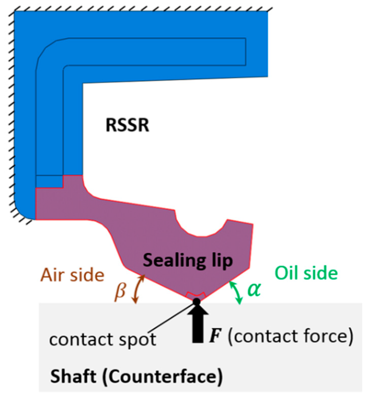
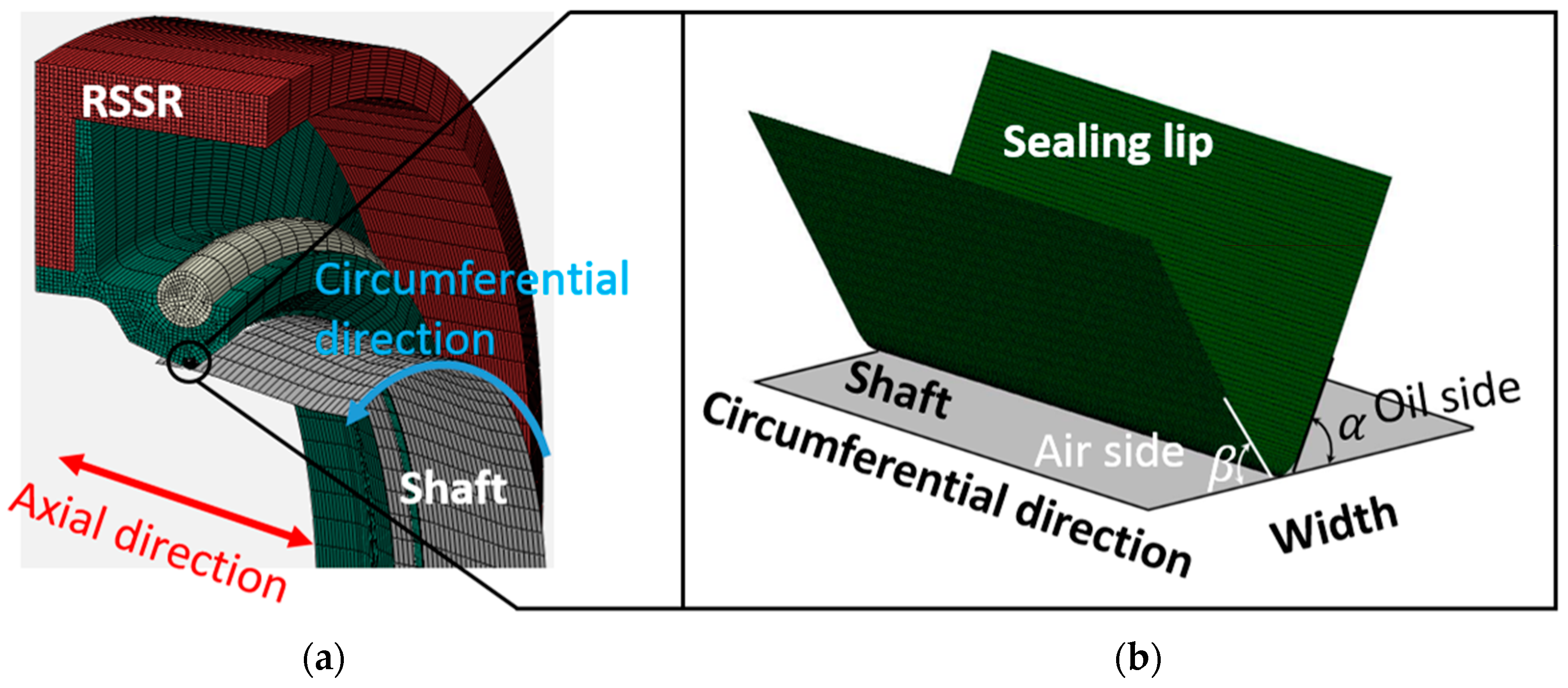
2.1. RSSR Tribological System

The RSSR tribological system essentially consists of three components: The sealing ring, the counter surface, and the lubricant. Figure 1 shows a sectional view of the contact between the elastomer sealing lip and the counter surface in the sealing system.
The good functionality of the RSSR system depends mainly on macro-geometric, micro-geometric, and operating parameters. In the following, some important influencing variables will be explained. The macro-geometry of the sealing lip is characterized by the different contact angles between the sealing edge and shaft on the air side β and oil side α . These different angles provide an asymmetrical contact pressure, which is an absolute condition for a good function. As example, in [18] the following value ranges 20–30° and 40–50° are recommended for the β and α angles in the unassembled state. While manufacturing shaft surfaces for RSSR systems, two requirements are imposed on the micro-geometry achieved. On the one hand, the manufactured surface should be twist free as much as possible. On the shaft surfaces, the twist structures resulting from standard manufacturing processes such as the turning process can have a negative pumping effect during operation depending on the rotation direction of the shaft and lead to leakage [20]. To avoid this, the shaft surfaces are further grinded after the turning process. On the other hand, the smoothness achieved by the grinding process from a critical roughness value can lead to problems. In fact, roughness profiles form so-called ‘‘pockets’’ on the shaft surfaces in order to maintain the lubricating film. Guidelines for the selection of surface roughness for shaft surfaces can be found in the standard International Organization for Standardization (ISO) 6194.
Depending on surface roughness and operating parameters (e.g., temperature, speed), various friction and lubrication conditions can occur in the sealing contact, which are difficult to predict. A popular friction model for sealing contact is the Engelke model, which will be briefly described hereafter. Engelke presented in [19] a model for the iterative calculation of the friction torque and contact temperature in the sealing contact based on a large number of experimental investigations. Here the total friction torque M r is summarized from the sum of a dry friction component M 0 and a viscous component   M η :
M r = M 0 + M η .
The dry friction component M 0 is determined from the radial force F r a d , the limiting friction value μ 0 , and the shaft radius r w as follows:
M 0 = F r a d · μ 0 · r w .
The viscous friction torque M η , on the other hand, is determined from the dynamic viscosity η ( T ) , which depends on the sealing contact temperature, the sealing contact width b , the sum of the mean roughness peaks in the contact R P (as an approximation of the lubricating film thickness), and the speed n :
M η = η ( T ) · b · r w 3 · 4 · π 2 · n R P .

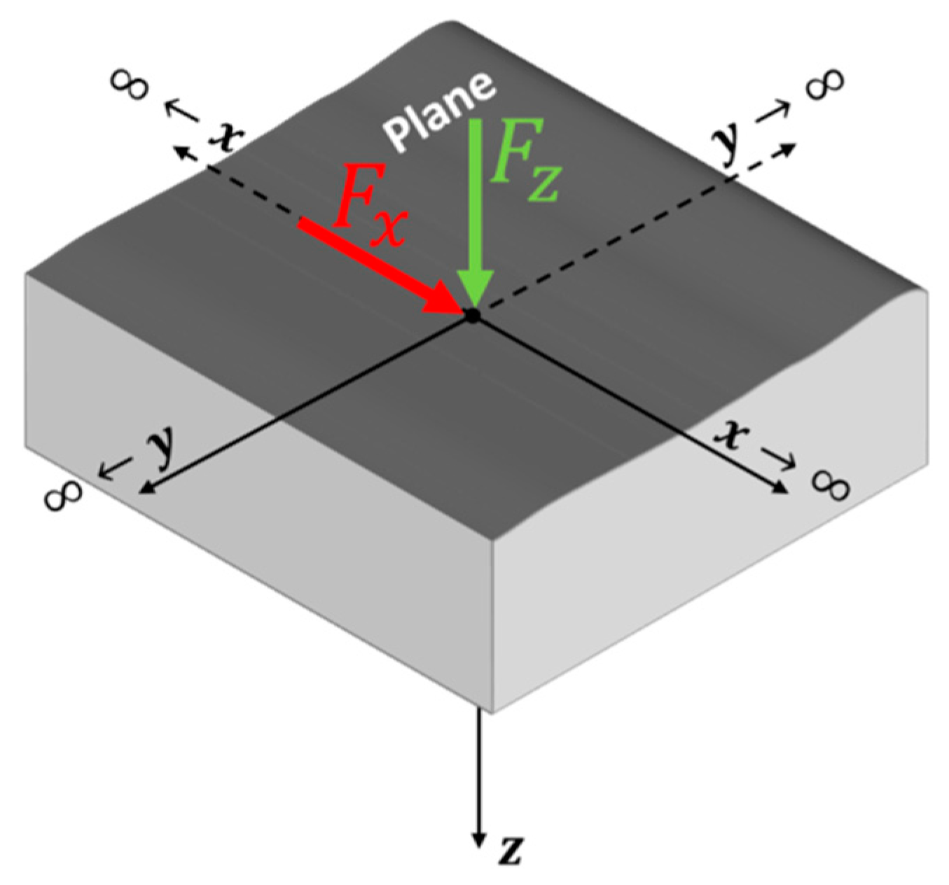
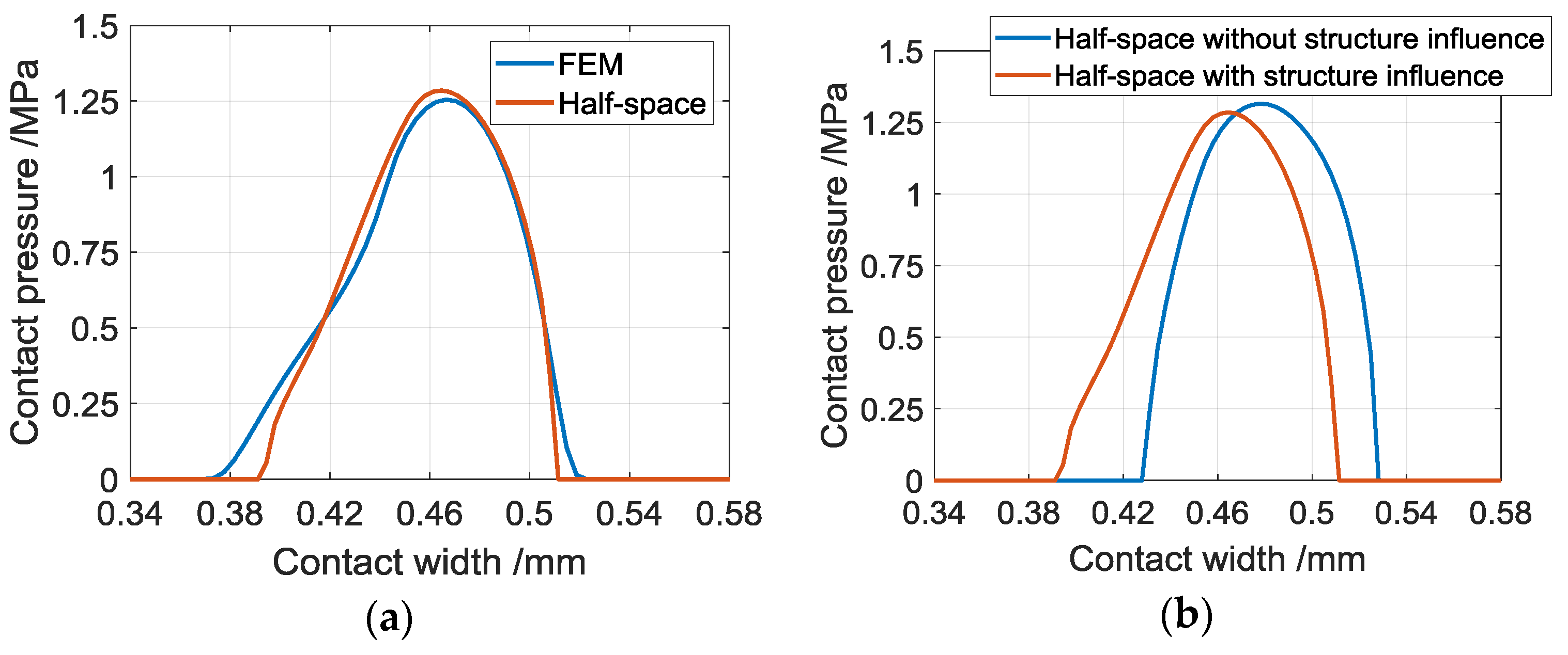
2.2. Half-Space Theory and Its Applicabiliy to RSSR Contact Problem

The semi-analytical contact model implemented in this work is based on the half-space theory, where contact bodies are considered as half-space. In continuum mechanics, a half-space describes a semi-infinite space bounded in one direction by a plane (see Figure 2). External forces can only act on the half-space via this plane.
Fundamental solutions on which most semi-analytical contact models are based are the Boussinesq and Cerruti solutions given in Equations (5) and (6) [21] for the displacements on the half-space on which, respectively, a normal F z and a tangential force F x act. From these fundamental solutions the coefficients of influence described in Section 3.1 were derived, which were used for the numerical implementation of the contact model.
      u B o u s s i n e s q = [ u x u y u z ] = ( F z   x 4 π G R [ z R 2 1 2 ν R + z ] F z   y 4 π G R [ z R 2 1 2 ν R + z ] F z   4 π G R [ 2 ( 1 ν ) z 2 R + z ] )
       u C e r r u t i e = [ u x u y u z ] = ( F x   x 4 π G R [ 1 + x 2 R 2 + ( 1 2 ν ) ( R R + z x 2 ( R + z ) 2 ) ] F x   x y 4 π G R [ 1 R 2 1 2 ν ( R + z ) 2 ] F x   x 4 π G R [ z R 2 + 1 2 ν R + z ] )
where R = x 2 + y 2 + z 2 .
The use of the half-space theory to resolve the contact problems presupposes basically the following assumptions:
  • Extremely small contact dimensions compared to body dimensions,
  • A linear elastic behavior of the contact bodies, and
  • No structural deformation influence on the contact problem.
From the three conditions mentioned above only the first one is in case of RSSR contact problem directly without further fulfilled. In fact, the contact in the RSSR system took place in a very small region (approx. 1 μm contact width) compared to the geometry dimensions of the sealing lip (see Figure 1). However, the sealing lip of the RSSR showed a hyperelastic material behavior and the bending of the sealing lip (structural deformation) had a big influence on the contact as the results show later. For these two last reasons, the material behavior of the sealing lip should be linearized (see Section 3.2) and the structural deformation influence on the contact should be determined beforehand (see Section 3.1) for the application of semi-analytical contact modeling to the RSSR contact problem.
The method described in Section 3.1 is based on the assumption of a linear elastic behavior of the sealing lip, which allows the superposition principle to be used to determine the contact displacements. The total contact displacement on the sealing lip is summarized as shown schematically in Figure 3, from a local deformation part (without macroscopic displacements) and a macroscopic structural deformation part (without local deformations) from the bending of the sealing lip. The structural deformation influence required to consider the second deformation part of the contact displacements in the half-space model was determined using a finite element model of the RSSR.

3. Semi-Analytical Frictional Contact Modelling of RSSR

As already mentioned in the introduction, the contact bodies are considered as half-spaces in the semi-analytical contact modelling approach. This simplification requires, among other things: A linear elastic behavior of the bodies and an infinitely wide dimensions of the bodies. From the latter condition, any structural deformation influences remained unconsidered at first. In this section, the first Section 3.1 presents the fundamental solutions of the displacements on a half-space and their extension for the RSSR contact problem by considering the bending of the sealing lip. In the second Section 3.2, the material parameters and contact surfaces geometry of the sealing lip and shaft are discussed. Finally, the main contact equations and the iterative solution scheme will be described in the last subsection.

3.1. Fundamental Solution on the Half Space for RSSR Contact Problem

The solution to the contact problem is an iterative determination of the contact displacement by checking previously defined contact conditions. The surface displacements on a half-space are obtained from the fundamental solutions of Boussinesq and Cerruti. For this purpose, the surface of each half-space (contact partner) and the load acting on it was discretized. Figure 4 shows, for example, the surface of the half-space discretized into N x × N y square segments with the dimensions 2 a , 2 b . For simplicity, only the normal contact is discussed in the following consideration. The normal surface load p k l is assumed to be constant for each surface element. The index k and l describe the position of the area load in the coordinate system.
In the case of a single point load, as shown in Figure 2, the normal displacement due to a normal load is given by the third component of the displacement field Equation (5):
u z = F z 4 π G R [ 2 ( 1 ν ) z 2 R + z ] .
On the surface (z = 0) results:
u z = 0 = F z 4 π G R [ 2 ( 1 ν ) ] .
With the following relationship G = E [ 2 ( 1 + ν ) ] between the shear modulus G and elastic modulus E , the relationship in Equation (8) can be simplified as follows:
u z = 0 = F z · ( 1 ν 2 ) π E R .
The quantity ( 1 ν 2 ) π E R in Equation (9) describes the coefficient of influence of a normal single point load F z on a normal displacement u z on the surface of a half-space. In order to describe the coefficient of influence for a surface load p k l z , the coefficient just derived in Equation (9) must be integrated over the surface segment (shown in Figure 4). The following integration formula was proposed by Love [22]:
C i j k l z z = b b a a ( 1 ν 2 ) π E R d x k d y l = ( 1 ν 2 ) π E b b a a 1 ( x i x k ) 2 + ( y j y l ) 2 d x k d y l = ( 1 ν 2 ) π E [ ( x i + a ) log ( ( x i + a ) 2 + ( y j + b ) 2 + y + b ( x i + a ) 2 + ( y j b ) 2 + y b ) + ( x i a ) log ( ( x i a ) 2 + ( y j b ) 2 + y b ( x i a ) 2 + ( y j + b ) 2 + y + b ) + ( y j + b ) log ( ( x i + a ) 2 + ( y j + b ) 2 + x + a ( x i a ) 2 + ( y j + b ) 2 + x a ) + ( y j b ) log ( ( x i a ) 2 + ( y j b ) 2 + x a ( x i + a ) 2 + ( y j b ) 2 + x + a ) .
The nomenclature used in Equation (10) was defined as the two superscripts zz indicating the direction of displacement and the area load, respectively. The four assumed indices describe in pairs the position of the area element where the displacement is currently being determined ( i , j marked red in Figure 4) and the position of the area load ( k , l marked blue in Figure 4). The expression for determining the normal displacement on any area element, j , due to an area load p k l z at point k , l can be written compactly as follows:
u i j z z = C i j k l z z · p k l z .
If several k l surface elements are subjected to normal loads p k l z , then the resulting normal displacement at one point i j results from the superposition of the individual contributions as follows:
U i j z z = k = 1 N x l = 1 N y C i j k l z z · p k l z .
The Equation (12) represents with regard to mathematical programming a convolution between the influence coefficients C i j k l z z as kernel function with the normal loads p k l z . This equation is solved was this work with the help of the Fourier transformation. First, the influence coefficients and normal loads presented as 2D matrix were transformed in the frequency domain. Here in the frequency domain the complex convolution operation was replaced by a simple matrix multiplication. The result of this multiplication was then retransformed in the space domain.
The relation in Equation (12) was further represented compactly with the operator as a convolution product as follows:
U i j z z = C i j k l z z p k l z .
In the case of a frictional contact problem, both normal loads p k l z (in z direction) and tangential loads q k l x ,   q k l y (each in x and y directions) act on each discrete surface element. These loads cause displacements in all three spatial directions x , y , z at any point i j on the half-space. The total displacement in x direction on a point i j for example, can be determined from the individual contributions of the loads ( p k l z , q k l x ,   q k l y ) as follows:
U i j x = U i j x x + U i j x y + U i j x z = C i j k l x x q k l x + C i j k l y y q k l y + C i j k l x z p k l z
The solutions for frictional contact problems are often described by full coupling of the normal and tangential behavior by the following relationship (derived from Equation (13)):
[ U i j x U i j y U i j z ] = [ C i j k l x x C i j k l x y C i j k l x z C i j k l y x C i j k l y y C i j k l y z C i j k l z x C i j k l z y C i j k l z z ] [ q k l x q k l y p k l z ] .
The following nomenclature clarifies the relationship Equation (15): The indices i j and k l , respectively, denote the coordinates of the evaluation points of the displacement and the load application point. The letters x , y , z describe the three spatial directions. With this fixed nomenclature, the meaning of the displacement influence coefficients becomes apparent. The influence coefficient C i j k l x x determined as example the displacement in point i j in spatial direction x caused by a tangential load q k l x oriented in spatial direction x and acting in point k l . Analytical expressions for the displacement influence coefficients can be found in [7,8,9,21]. The determination of the displacements on the sealing lip with the relation Equation (15) was imprecise due to the high structural influence (here the bending of the sealing lip in Figure 3b) on the resulting contact displacements. For this reason, the structural influence matrices ( S i j k l x x ,   S i j k l y y ,   ,   S i j k l x y ) were first determined by finite element analysis (FEA) and added to the influence coefficients in Equation (15). The method for determining the structural influence matrices is described in [23,24] for the gear contact. The main steps by the implementation of this method for the sealing contact are explained in further.
The FE model used for this purpose was the simulation model in [17] (see Figure 5) built in finite element software Abaqus. The sealing edge of the sealing lip was finely meshed with N nodes as shown in Figure 5.
Under the assumption of small linear elastic deformations, the superposition principle was applied and the total contact displacement u t o t a l is summarized as follows from a local part u l o c a l and a part from the structural bending of the sealing lip u s t r u c :
u t o t a l = u l o c a l + u s t r u c .
The displacement component due to structural deformation can be determined from Equation (16) as follows:
u s t r u c = u t o t a l u l o c a l .
With the displacement component from Equation (17), the desired structural influence matrices can be determined as described in [23,24]. The Equation (17) was solved with the help of two simulation series with different boundary conditions for u t o t a l and u l o c a l . These boundary conditions are described hereafter. The determination of the total displacement u t o t a l required a free movement of the sealing lip. This was made possible by the boundary condition shown in the Figure 6a. On the contrary, for determination of the local displacement u l o c a l , the bending of the sealing lip must be prevented by an additional boundary condition (see Figure 6b).
With the structural influence matrices ( S i j k l x x ,   S i j k l y y ,   ,   S i j k l x y ) as already described, the total displacement field on the sealing lip was determined in the semi-analytical contact model as follows:
[ U i j x U i j y U i j z ] = [ C i j k l x x + S i j k l x x C i j k l x y + S i j k l x y C i j k l x z + S i j k l x z C i j k l y x + S i j k l y x C i j k l y y + S i j k l y y C i j k l y z + S i j k l y z C i j k l z x + S i j k l z x C i j k l z y + S i j k l z y C i j k l z z + S i j k l z z ] [ q k l x q k l y p k l z ] .
The structural deformation influence coefficients obtained from the method briefly described above are only valid for specific sealing lip contact geometry and cannot be applied to other geometries.

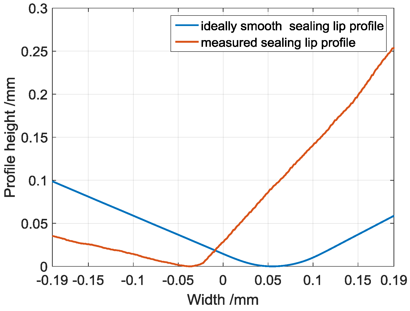
3.2. Material Parameters and Contact Surface Geometry for the Simulation

In addition to the experimental friction torque values described in Section 5, the important simulation parameters are the geometry and material parameters of the shaft and elastomer sealing lip. This paper assumes a steel shaft made of 16MnCr6 according to German Institute for Standardization (DIN) 3761. In comparison to the shaft, the sealing lip showed a hyperelastic behavior. The nonlinearity in the material behavior of the elastomer made it difficult to model the sealing lip with the half-space theory, since this basically assumed a linear elastic behavior. For this reason, this paper assumed small deformations of the sealing lip and a linear elastic material behavior. The modulus of elasticity of the sealing lip for the simulation can be determined from two ways: Directly from a step tensile test as done in [18], or from the Mooney Rivlin parameters, C10 and C01, if these were already determined. For the second variant, the approximation formula proposed according to Equation [14] was used:
E e l a s t o m e r = 6 ( C 10 + C 01 ) .
In this paper the first determination method was preferred and a modulus of elasticity for the elastomer from the step tensile test as done in [18] was used. Due to the incompressibility of the elastomer material, the model considered a Poisson’s ratio of 0.49 . Table 1 summarizes the material parameters and some geometric values used in the simulation for both contact partners.
The simulation model required the contact surface of the sealing lip and the shaft. The RSSR and the shaft (see Figure 7a) were both thoughtfully cut in axial directions and unwound over their circumference (see Figure 7b).
This paper assumed an idealized case with an axially symmetrical geometry of the sealing lip, i.e., with constant cross-sectional profile over the circumference, as shown in Figure 7b. In the simulation, both ideally smooth and measured sealing lip profiles were used (see Figure 8). The determination of the structural deformation matrix under consideration of the real sealing lip profile with sufficient accuracy by means of an FE model posed a great challenge due to the very long computing time for a sufficiently fine meshing of the real sealing lip profile. This effort could not be accomplished within the time frame of this publication but will be done in future works. For the simulation with real sealing lip profile, the profile geometry of a sealing lip was measured at four different angles in circumferential directions and the averaged profile was used in the axially symmetric model. As an example, Figure 8 shows the averaged profile for the Fluorinated rubber (FKM) sealing lip compared to the ideally smooth profile.

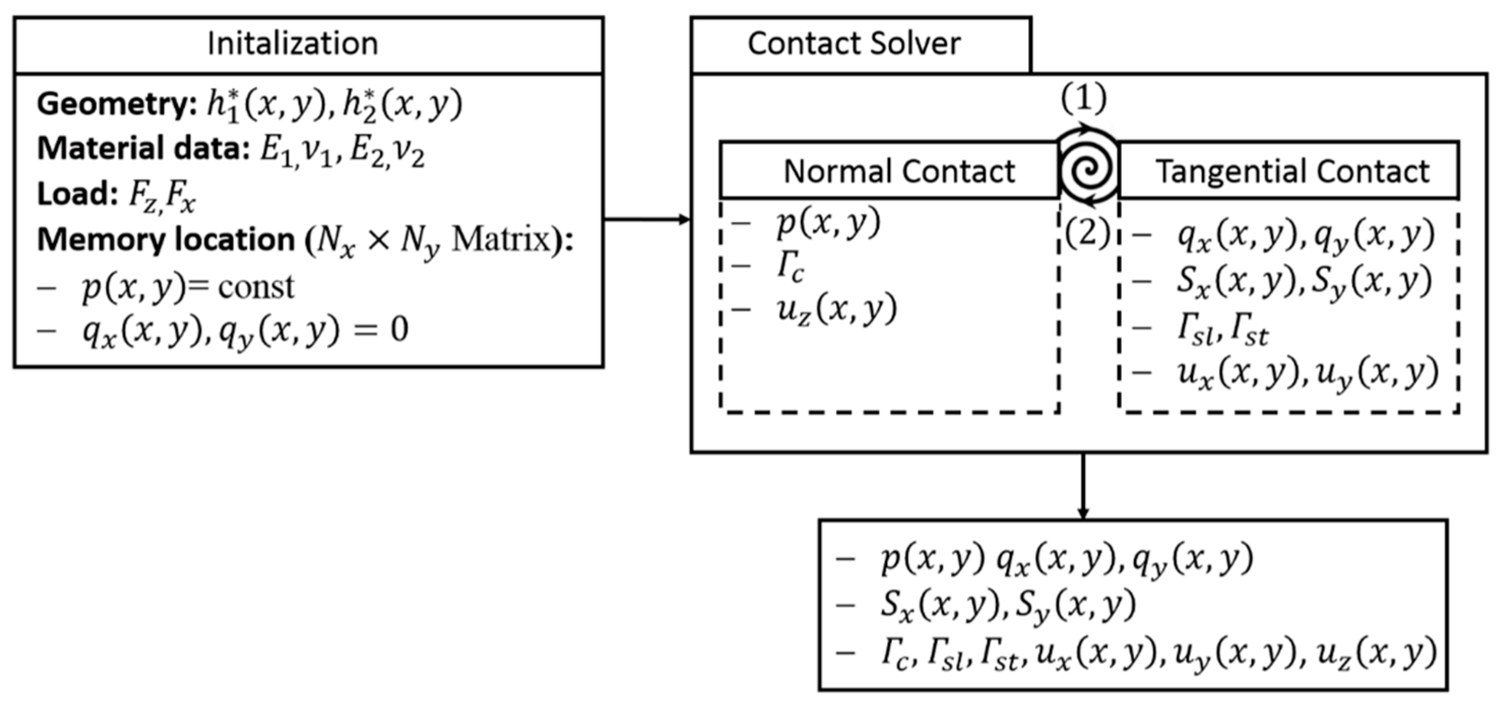
3.3. Contact Conditions and Itterative Solution Scheme

After describing the coefficient of influence to determine the displacements on a half-space taking into account the structural deformation as made in the first section and presenting the geometry and material parameters used in the contact model, this section presents the contact conditions and the solution scheme of the contact algorithm.
To describe the normal and tangential contact conditions, the contact problem between two elastic bodies (K1, K2) under normal and tangential force F z , F x shown schematically in Figure 9a was used. For simplicity’s sake, the two sectional views in Figure 9b,c were used. For an easy recognition of belonging of the geometric variables, the two surface profiles are represented with different colors (blue for K1 and red for K2). Despite the two dimensional representation in Figure 9b,c, which is only for illustrative purposes, the following description was made for the general case of a three-dimensional contact problem. In order to avoid confusion, the parenthetical expression ( x , y ) was used for three-dimensional variables.
As can be seen in the sectional view in Figure 9b, the normal contact has the following parameters:
  • F z : Normal force (radial force on sealing lip)
  • h i 1 ( x , y ) ,   h i 2 ( x , y ) : Surface profile heights of bodies 1 and 2
  • δ z 1 ,   δ z 2 : Body displacement of bodies 1 and 2 in normal direction, and
  • P 1 ,   P 2 : Centers of gravity of bodies 1 and 2,
In three-dimensional normal contact, the following conditions must be applied:
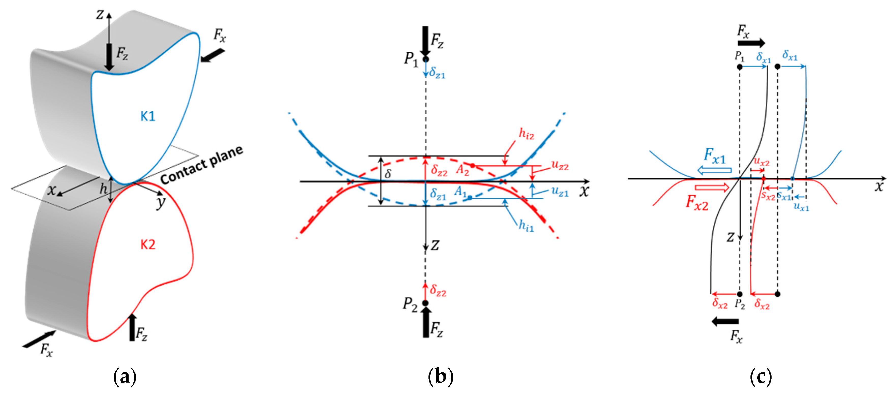
  • The equilibrium. It forms an equivalent relationship between the externally applied normal force F z and the normal pressures p to be determined in the contact region Γ c :
    F z = Γ c p ( x , y ) d Γ c
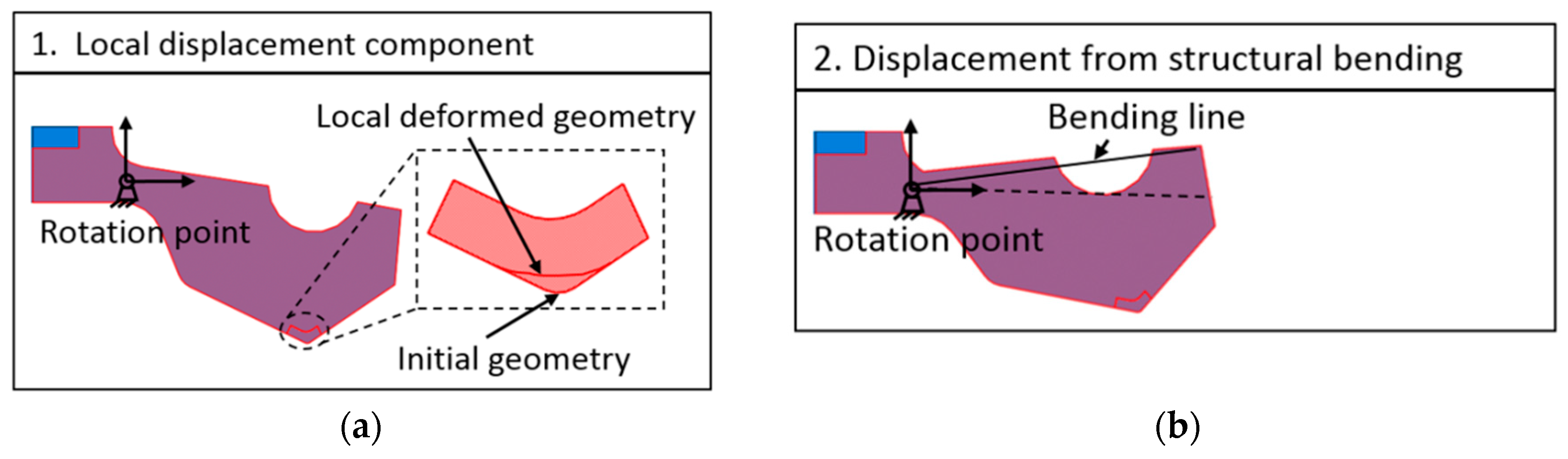
  • The gap equation. This equation describes the change of the contact gap h ( x , y ) (distance between the contact bodies). Two cases are shown in Figure 9b to explain the gap equation. In the first case, the two contact bodies, K1 and K2, were considered as rigid bodies. Thus, their surface profiles remained undeformed (see dotted lines). Here, the centers of gravity under the contact force F z made the body displacements δ z 1 ,   δ z 2 . As help geometry, tangent lines were formed as reference lines in the deepest profile points. In the second case, the two bodies were represented in a deformed state (see strong lines). At the origin ( x = 0 ), the vertical distances from the contact point to the reference lines described the body displacements δ z 1 ,   δ z 2 mentioned in the first case. The gap at any contact point pair was described by the initial profile height h i ( x , y ) (point distances to the respective reference lines in the nondeformed state) and the displacements u z ( x , y ) (distance changes from the nondeformed to the deformed state) as follows:
    h ( x , y ) = ( h i 1 ( x , y ) + h i 2 ( x , y ) ) ( δ z 1 + δ z 2 ) + ( u z 1 ( x , y ) + u z 2 ( x , y ) ) .
  • The complementarity condition. This condition arises due to the impenetrability of the contact bodies. It links the contact gap h ( x , y ) Equation (21) and the contact pressure p ( x , y ) Equation (20) as follows:
    if h ( x , y ) > 0 p ( x , y ) = 0         ( x , y )   Γ c else h ( x , y ) = 0 p ( x , y ) > 0         ( x , y )   Γ c .
The formulation of the tangential contact, as described below, required more consideration than the normal contact. Here, the contact region Γ c was divided into two areas, a sticking region Γ s t and a sliding region Γ s l . The tangential contact conditions were described using the sectional view in Figure 9c. The tangential contact had the following parameters:
  • F x : Tangential force (friction force on sealing lip),
  • F x 1 , F x 2 : Action-reaction forces on bodies 1 and 2,
  • u x 1 ( x , y ) , u x 2 ( x , y ) : : Surface displacement of bodies 1 and 2,
  • δ x 1 ,   δ x 2 : Body displacement of bodies 1 and 2, and
  • P 1 ,   P 2 : Centers of gravity of bodies 1 and 2.
In Figure 9c, a tangential force F x was introduced into the contact region ( F x 1 on body 1 and F x 2 on body 2) and caused similar to the case of the normal contact (see Figure 9b) on the body centers of gravity the body displacements δ x 1 and δ x 2 in the tangential x-direction. For each contact point pair in the sticking region (center of the contact zone), Γ s t the body displacements of the center of gravity δ x 1 , δ x 2 were equal to the surface displacements u x 1 ( x , y ) ,    u x 2 ( x , y ) . Thus, the contact point pair remained on the same x -coordinate after the deformation. In the sliding region (at the boundary of the contact zone), Γ s l , on the other hand, the difference between the body displacements δ x 1 , δ x 2 and the surface displacements u x 1 ( x , y ) , u x 2 ( x , y ) resulted in sliding paths s x 1 ( x , y ) , s x 2 ( x , y ) .
In general, the following three-dimensional tangential contact conditions must be applied:
The equilibrium in the tangential directions:
F x = Γ c q x ( x , y ) d Γ c F y = Γ c q y ( x , y ) d Γ c ( x , y ) Γ c ,
The sliding equation in the sliding zone Γ s l , which expresses the sliding paths from the surface displacement u x ( x , y ) , u y ( x , y ) and the body displacement δ x , δ y as follows:
S ( x , y ) = ( S x ( x , y ) = u x ( x , y ) δ x S y ( x , y ) = u y ( x , y ) δ y ) ; ( x , y ) Γ s l ,  
The Coulomb’s friction law, which limits the magnitude of the shear stress Q in the adhesive area Γ s t by using the coefficient of friction μ and the normal pressure p and reads:
| | Q ( x , y ) | | = ( q x ( x , y ) ) 2 + ( q y ( x , y ) ) 2 μ   · p ( x , y ) ; ( x , y ) Γ s t .
If the tangential body displacements δ x ,   δ y in Equation (20) were several orders of magnitude higher than the surface displacements u x ( x , y ) ,   u y ( x , y ) , then the tangential problem changes from a contact with partial sliding to a contact with full sliding. Such a case occurred in the contact between the seal lip and the counter surface during operation. In this case, the sliding Equation (24) was replaced by the following energy equilibrium [12]:
Γ c q x · S x ( x , y ) d Γ c = E d x Γ c q y · S y ( x , y ) d Γ c = E d y .
By using Equation (26), the sliding paths,   S x ( x , y ) ,   S y ( x , y ) , were determined from the friction energies E d x , E d y . As in this work, the friction energies can be determined experimentally.
The above described contact conditions and implementation of the contact algorithm for a friction contact problem with partial and full sliding are described in detail in the literature [4,12]. The method presented there was implemented in this work and will be briefly described in herein. The solution of the contact problem began with its formulation as a minimization problem with constraints. The contact conditions described were applied as constraints. The algebraic system of equations derived from the minimization problem was solved with the conjugated gradient method (CGM). The use of CGM gave the algorithm a fast convergence and thus a short calculation time. The implementation of the contact algorithm was done in this work with the software Matlab version 2015b.
As a summary, Figure 10 schematically shows the general solution flow of the frictional contact problem with partial or full sliding. At the beginning, geometric variables, such as the body geometry of the contact partners (in the sealing system the counter face h 2 and the sealing lip h 1 ), the material properties, and the external loads, were defined in the initialization step. As normal load F z in the sealing contact, the radial force values determined experimentally in the Table 1 were used. In the tangential direction, either the tangential load F x (friction force) for the contact with partial sliding or the friction work in case of full sliding can be defined. In the sealing contact, full sliding takes place during wear. From this, the experimentally determined friction work E d (see Section 5) was used in this work in the tangential direction. In order to avoid an automatic overestimating of the required storage space in Matlab, storage spaces were defined in the form of N x × N y 2D matrices (for a N x × N y calculation area). The normal contact pressure p ( x , y ) and the shear stresses q x ( x , y ) , q y ( x , y ) were initialized with different values. A meaningful starting value for the contact pressure was determined from the normal load and the total area as follows:
p ( x , y ) = c o n s t = F z N x · N y · a · b    .
The shear stresses matrices q x ( x , y ) , q y ( x , y ) , on the other hand, were all set to zero at the beginning. This value can be justified by the fact that in the contact solver the normal contact is solved first.
After the initialization, the contact solver started. There were two main interaction steps between the normal and the tangential problem. First, the shear stresses q x ( x , y ) , q y ( x , y ) (from the tangential problem) caused displacements in the normal direction u z ( x , y ) and, thus, influence the normal contact pressure p ( x , y ) , which was determined in the normal contact. On the other hand, the normal contact pressure influenced the tangential displacements u x ( x , y ) , u y ( x , y ) . This mutual influence is represented in Figure 10 by the arrow directions 1 and 2.
At the end of the contact simulation, the following variables were determined:
  • The contact region: Γ c ,
  • The sliding and adhesion zone: Γ s l , Γ s t with Γ c = Γ s l Γ s t ,
  • Normal pressure: p ( x , y ) ,
  • Shear stresses: q x ( x , y ) , q y ( x , y ) ,
  • Surface displacements: u x ( x , y ) , u y ( x , y ) ,   u z ( x , y ) ,
  • Body displacements: δ x , δ y , δ z , and
  • Sliding paths: S x ( x , y ) , S y ( x , y ) .
As will be described in Section 4, the wear rate at each contact point was obtained from the shear stresses q x ( x , y ) , q y ( x , y ) and sliding paths   S x ( x , y ) , S y ( x , y ) using Equation (30).

4. Wear Calculation

Various approaches exist for the calculation of wear according to the current state of the art. These can be divided into two main groups. The first group is that of the classical wear theories. This includes the pressure-based wear law according to Archard [17,25]. According to this model, the wear volume can be determined as follows:
V = α A · s · p H .
where α A , s ,   p , and H correspond to the wear coefficient, the sliding distance, the normal pressure, and the hardness of the soft contact partner, respectively. While this wear model has the advantage of being easy to implement, it has the disadvantage of not taking into account many critical parameters such as the friction condition. In the second group of modern wear models, the friction energy-based wear model according to Fleischer [18,26], which was used in this paper, is classified. Here the wear equation is:
V = α F · E d = 1 e R · E d .
With α F , e R , and E d as wear coefficient, friction energy density, and the friction work, respectively.
Here the wear coefficient was calculated from the reciprocal of the friction energy density, which was determined experimentally. The friction work E d in Equation (29) can also be determined from experiments.
In this work the friction work was determined from experimentally measured friction torques on the shaft. The friction work was the main input variable for the contact algorithm to determine the shear stresses q x ( x , y ) ,   q y ( x , y ) and the sliding paths S x ( x , y ) , S y ( x , y ) . The following local wear formulation is derived from Equations (26) and (29) [12]:
Δ h ( x , y ) = α F · E d = 1 e R · [ q x ( x , y ) q y ( x , y ) ] · [ S x ( x , y ) S y ( x , y ) ]
with Δ h as wear increment (local height change after wear).
In the wear simulation, the geometry of the contact partners was updated after each contact calculation step using Equation (30). Due to the use of Coulomb’s friction law (25) to determine the shear stresses used in Equation (30), this wear formulation offered the possibility to consider the friction condition compared to the Archard model. For the simulation in this work, a speed-dependent friction coefficient was used. This was determined from the ratio between an experimental speed-dependent tangential force value and the radial force measured in the new state (unworn) at the start of the experiment (see Table 2). The use of a constant radial force represented a simplification, as can be seen in Table 2, from the difference between the measured radial force before and after the test. In reality, a reduction in radial force occurred during operation due to wear and temperature-dependent material changes.

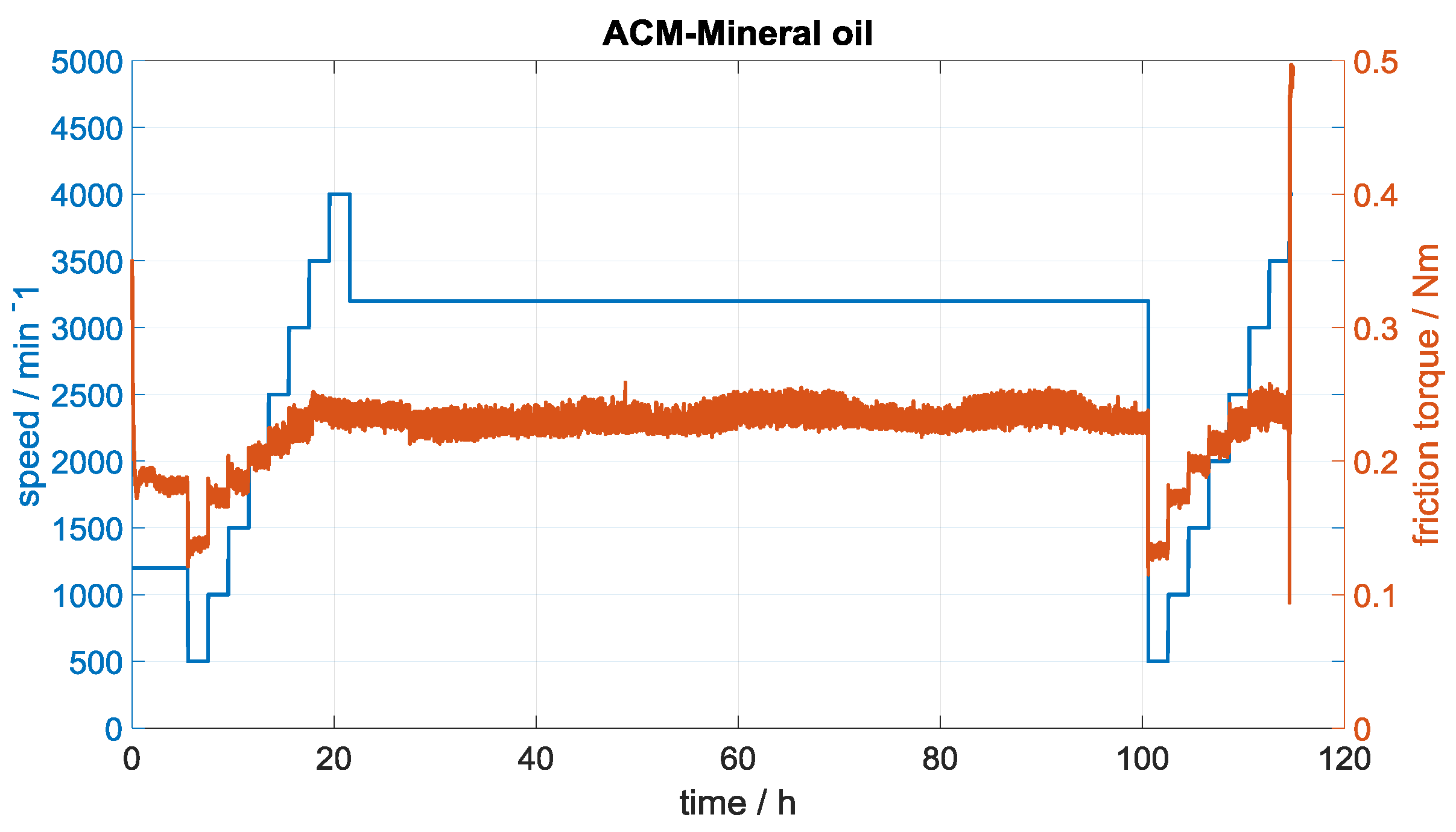
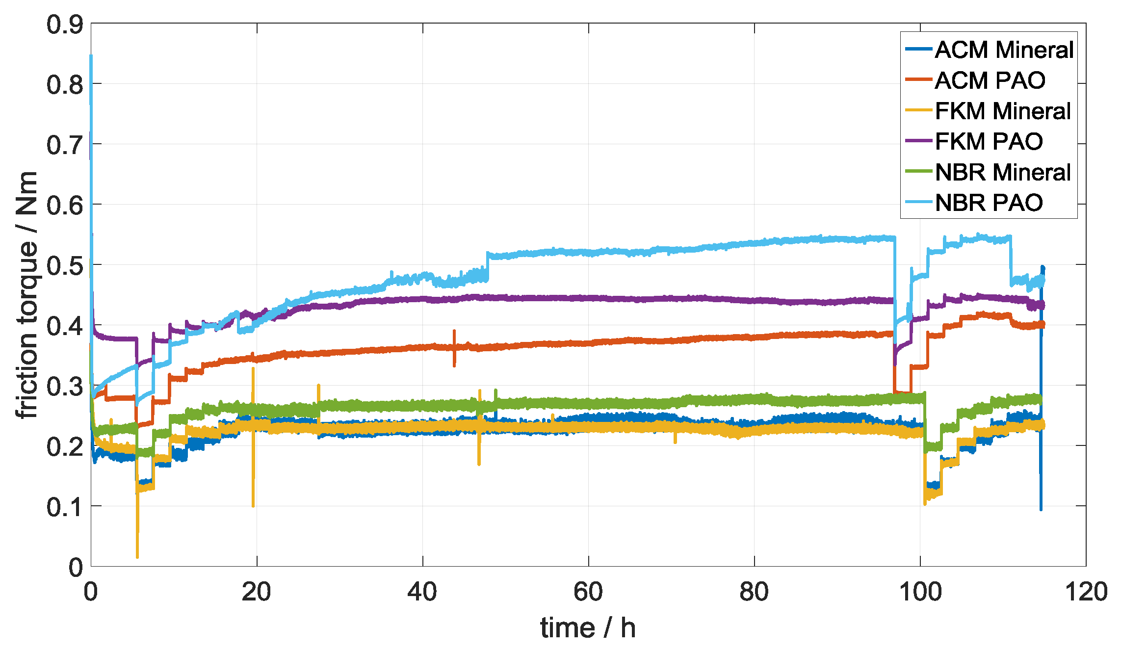
5. Experimental Determination of the Friction Work

The experimental determination of the friction work on the sealing system was herein carried out on a multi-shaft test stand with friction torque sensor [27]. For various combinations of elastomer materials (NBR, nitrile rubber; ACM, polyacrylate rubber, and FKM, fluorinated rubber) and lubricants (mineral oil and polyalphaolefin (PAO)), the friction torque on the shaft was measured in a speed- and temperature-controlled wear test. The wear distance for each test carried out in this work was 5000 km. After a running-in distance of 100 km at a speed of 1200 min−1, various speed levels from 500 to 4500 min−1 were run down. The stages were kept constant for two hours. The elastomer-lubricant combination was then run at a speed of 3200 min−1 in order to promote wear through prolonged constant loading. The speed steps at the beginning of the test were then repeated. As an example of the measurement result for the elastomer material made of ACM with the lubricant mineral oil, the friction torque curve in Figure 11 is shown.
With the use of the diameter of the test shaft D W , the friction force curve F r ( t ) can be determined from the friction torque curve M r ( t ) using the relation Equation (31).
F r ( t ) = 2 M r ( t ) D W
The friction work was determined by integrating the friction force progression Equation (31) over the sliding distance   s . The total friction work was determined via the individual speed stages and then summed up. The infinitesimal friction work d W of a time-varying force F r ( t ) can be determined as follows:
d W = F r ( t ) · d s
with d s as an infinitesimal sliding path. This can be calculated for the rotating shaft in the sealing system from the shaft radius and the shaft speed:
d s = 2 π · n · r w · d t .
For each speed stage with constant speed applied:
d W = 2 π   n   r w t 1 t 2 F r ( t ) · d t .
With Equation (34), the friction work at each speed stage was determined by time integration of the friction force curve F r ( t ) from the start of the stage (at time t 1 ) to the end (at time t 2 ) and used in the contact simulation.
In this work RSSR without spring of the design BAUM 5 × 780 × 100 × 10 mm from the manufacturer Freudenberg were used. Six elastomer–lubricant combinations were investigated (see Table 2). Figure 12 shows the experimentally determined friction torque curves for these combinations. Table 2 summarizes important experimental input data for the simulation.
The wear energy density was calculated from the measured friction work and wear volume at the sealing edge. The wear volume was determined by observing and measuring the contour of the sealing edge before and after the tests using a 3D microscope. The difference between the unworn and the worn profile curve was the planimetric wear surface. The wear volume was determined by rotating this wear surface around the geometric center of gravity [18,27].

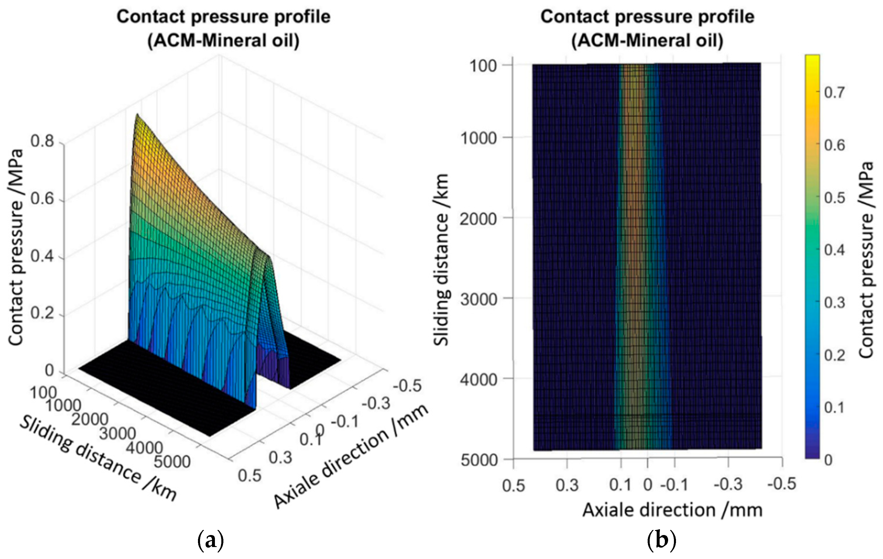
6. Simulation Results

The simulation results are presented in this section. In the first part, the results obtained with the ideally smooth sealing lip profile will be presented. In the second part a special attention is given to the combination FKM–mineral oil. The simulated contact pressures and the profiles changes in both cases with measured and ideally smooth sealing lip profile will be compared. Finally, the simulated profile change on the measured sealing lip profile in its new state is compared with the measured sealing lip profile at the end of the experimental wear test.

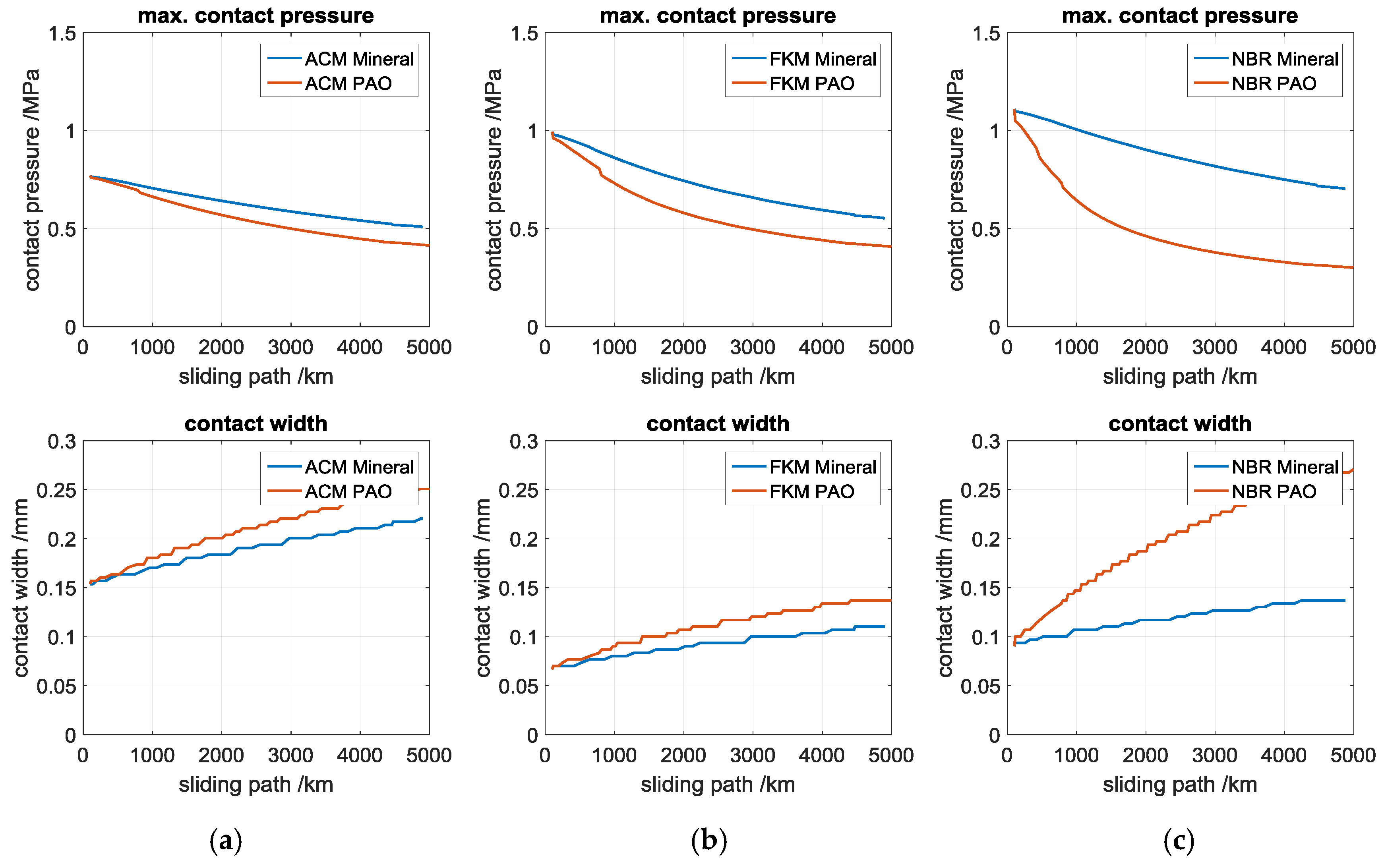
6.1. Simulation Results with Ideally Smooth Sealing Lip Profile

An essential step in the wear simulation was the exact determination of the contact pressures. As shown in Figure 13, these were significantly influenced by the structural bending of the sealing lip. This influence was determined for the ideally smooth sealing lip profile by a previously performed FEA and taken into account in the contact model Equation (18).
In the first step, the calculated contact pressure was verified in this section. The FE model [17] was used as the basis for comparison. Figure 13a shows a good agreement between both models, FE and half-space. The influence of structural deformation on contact pressure and contact width can be derived from Figure 13b. This figure compares the calculated contact pressures with and without structural influence. The structural deformation led to a reduction of the contact pressures from 1.350 to 1.2847 MPa (approx. 4%) and at the same time to an increase of the contact width from 0.1003 to 0.1204 mm (approx. 20%).
Figure 14 shows the results of the simulation with experimental friction torque values from the combination of ACM mineral oil. Two different views ((a) side view and (b) top view) show the contact pressure profiles for any section in the circumferential direction over the sliding distance. At the beginning there were high contact pressures with a maximum value of 0.770 MPa. However, these became smaller with increasing sliding distance down to a maximum value of 0.507 MPa (see Figure 14a). This decrease in contact pressures was favored, as can be better seen in the second view (see Figure 14b), by an increase in the contact width. In Figure 14b (in the top view) the size of the contact width can be can be identified in color through the area with positive contact pressures. From the beginning at 100 km sliding distance to the end of wear at approx. 5000 km, the contact width grew from 0.154 mm to 0.220 mm.
The comparison of the individual elastomer in combination with mineral oil and PAO is carried out in Figure 15. This shows the tendency towards higher wear (identifiable by the large decrease in contact pressure or increase in contact width) when combined with the lubricant polyalphaolefin (PAO). These results are in line with the friction torque curves in Figure 12, where higher wear was to be expected at higher friction torque values.
The results of the wear simulation in Figure 16a show good matches with the experimentally determined wear volumes for all elastomer–lubricant combinations except for the combinations with NBR elastomer. The large deviations in the results for NBR elastomer could either result from measurement errors at the torque sensor, which then led to errors in the simulation input variables, or from measurement inaccuracies in the experimental measurement of the wear volume. An exact measurement of the contact width was also very difficult due to the extremely small dimensions and the large scattering. This could be the reason for the large deviations between simulative and experimental values in Figure 16b. A significant advantage of the presented modeling approach is the short computation time, made possible by the use of the conjugated gradient method as equation solver in the semi-analytical contact model. As an example, the calculation times for the simulation of the six elastomer–lubricant combinations for a calculation area of 255*255 points were 371, 658, 318, 870, 355, and 1278 seconds, respectively.

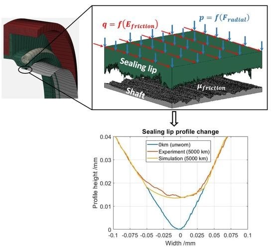
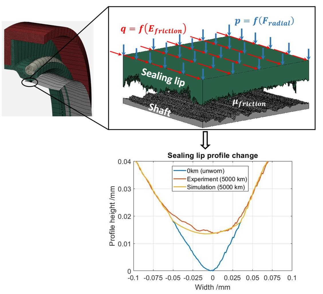
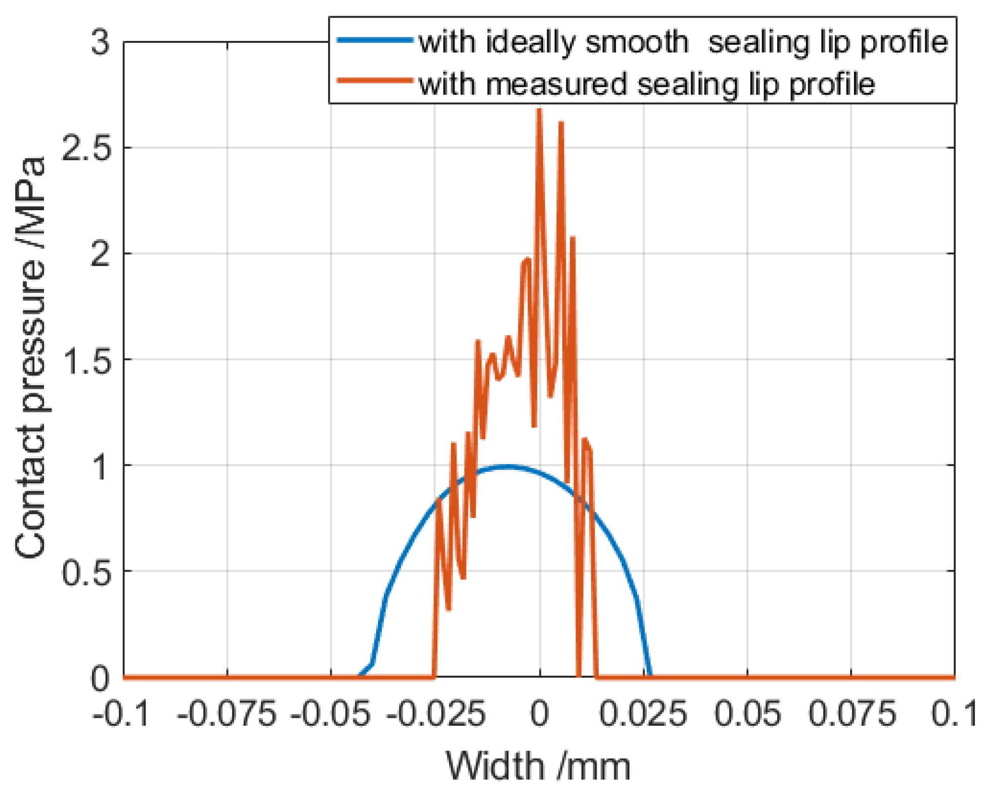
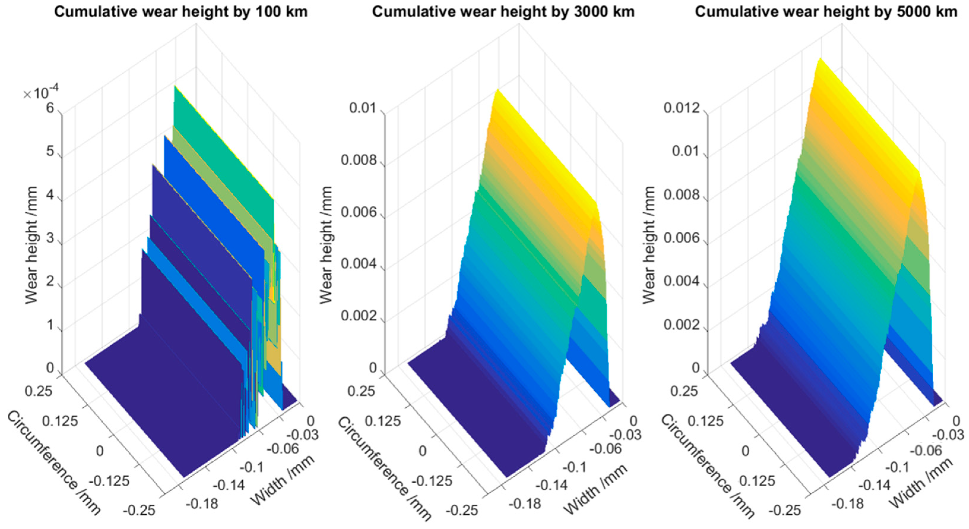
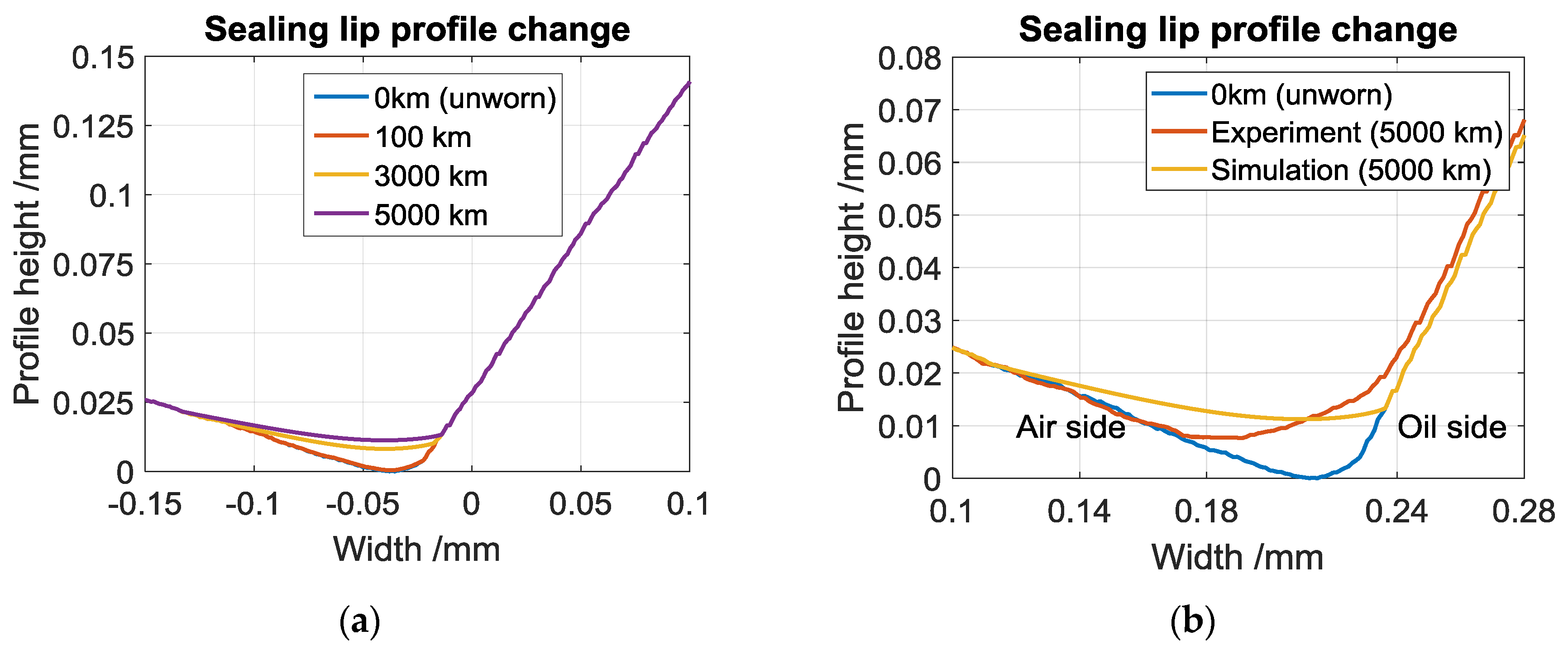
6.2. Simulation Results with Mesured Sealing Lip Profile for FKM-Mineral Oil Combination

Figure 17 compares contact pressures for an FKM elastomer with an ideal smooth and measured sealing lip profile. These were simulated with a normal force of 12.723 N. There was a large difference in the contact pressures. These differences could be due to the unconsidered structural influence matrices in the simulation with the measured profile. In fact, as can be seen from the comparison in Figure 13b, the structure deformation of the sealing lip led to more contact compliance and, thus, to a reduction in contact pressure.
An important benchmark is the profile change during and especially at the end of the wear simulation. This was obtained using Equation (30) from which the wear height increment was determined at each calculation step. Figure 18 shows, for example, for the combination FKM–mineral oil with the measured sealing lip profile, the cumulative wear height values after 100 km, 3000 km, and 5000 km sliding distance. As expected, there were small wear values at the beginning at 100 km (running-in), that increased as the sliding distance increased. The profile changes shown in Figure 19a were determined from these wear height values shown in Figure 18.
Figure 19b shows a comparison between the simulated and experimentally measured sealing lip profile after 5000 km sliding distance. The measured sealing lip profile after 5000 km sliding distance compared to the unworn shows a pronounced wear in the direction of the oil-side sealing edge. This effect was not completely reproduced by the simulation model. The simulated wear profile, instead, showed a more pronounced wear profile to the air side. This difference in the orientation of the wear area could be due to the unconsidered structural deformation influence. This can be explained by the influence of structural deformation on contact pressures shown in Figure 13b. When the structural deformation influence is taken into account, an asymmetrical shift of the contact pressure in the direction of the oil side is shown here and this results in more wear on the oil side.

7. Conclusions

Based on experimental friction torque values and a contact simulation, a model for estimating the wear on RSSR was presented in this paper. In the first step, the calculated contact pressures were verified with FE results and a good agreement was found. Despite the indirect consideration of the lubricant influence in the contact model by the friction energy density, a good agreement between experimentally and simulative determined wear volumes could be determined for most simulated elastomer lubricant combinations. The modelling approach presented here was particularly advantageous with regard to the short calculation time (maximum 21 min). In this work the assumption was made that the measured total friction torque contributed to wear and, thus, neglected the influence of the lubricant. However, with increasing speed, an ever larger lubricating film built up in the contact, so that a large part of the measured total friction torque was caused by the lubricant. In future work, this influence of the lubricant can be taken into account either experimentally (e.g., by measuring the churning loss) or by coupling a hydrodynamic simulation model into the contact simulation. Due to the unconsidered structural deformation influence matrix, the changes of the sealing lip profile during wear could not be properly simulated. The determination of the structural deformation matrix for the real sealing lip geometry by FEA can be the goal of future work.

Author Contributions

Conceptualization, F.F.F. and B.M.; methodology, F.F.F.; software, F.F.F.; validation, F.F.F. and J.H.; formal analysis, F.F.F.; investigation, F.F.F.; resources, J.H.; data curation, F.F.F.; writing—original draft preparation, F.F.F.; writing—review and editing, F.F.F.; visualization, F.F.F.; supervision, B.S.; project administration, B.S.; funding acquisition, B.S. All authors have read and agreed to the published version of the manuscript.

Funding

This research was funded by German Research Foundation (DFG).

Acknowledgments

The authors would like to thank the German Research Foundation (DFG) for the support of the research within the Collaborative Research Centre 926 “Microscale Morphology of Component Surfaces” (MICOS), Project-ID 172116086-SFB 926.

Conflicts of Interest

The authors declare no conflict of interest.

Nomenclature

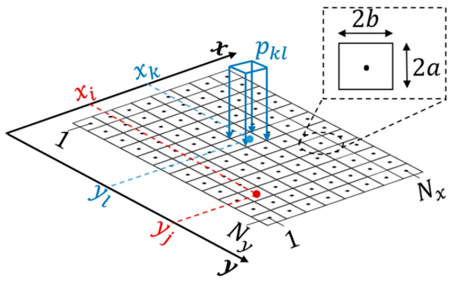
Discretization and indices
x , y , z ; i j , k l Spatial directions; position of a discretization point on the surface
N x , N y :Number of discretization points in X- and Y- spatial direction
contact calculation
F z , F x , F y ;Contact forces in normal direction (Z) and tangential directions (x,y)
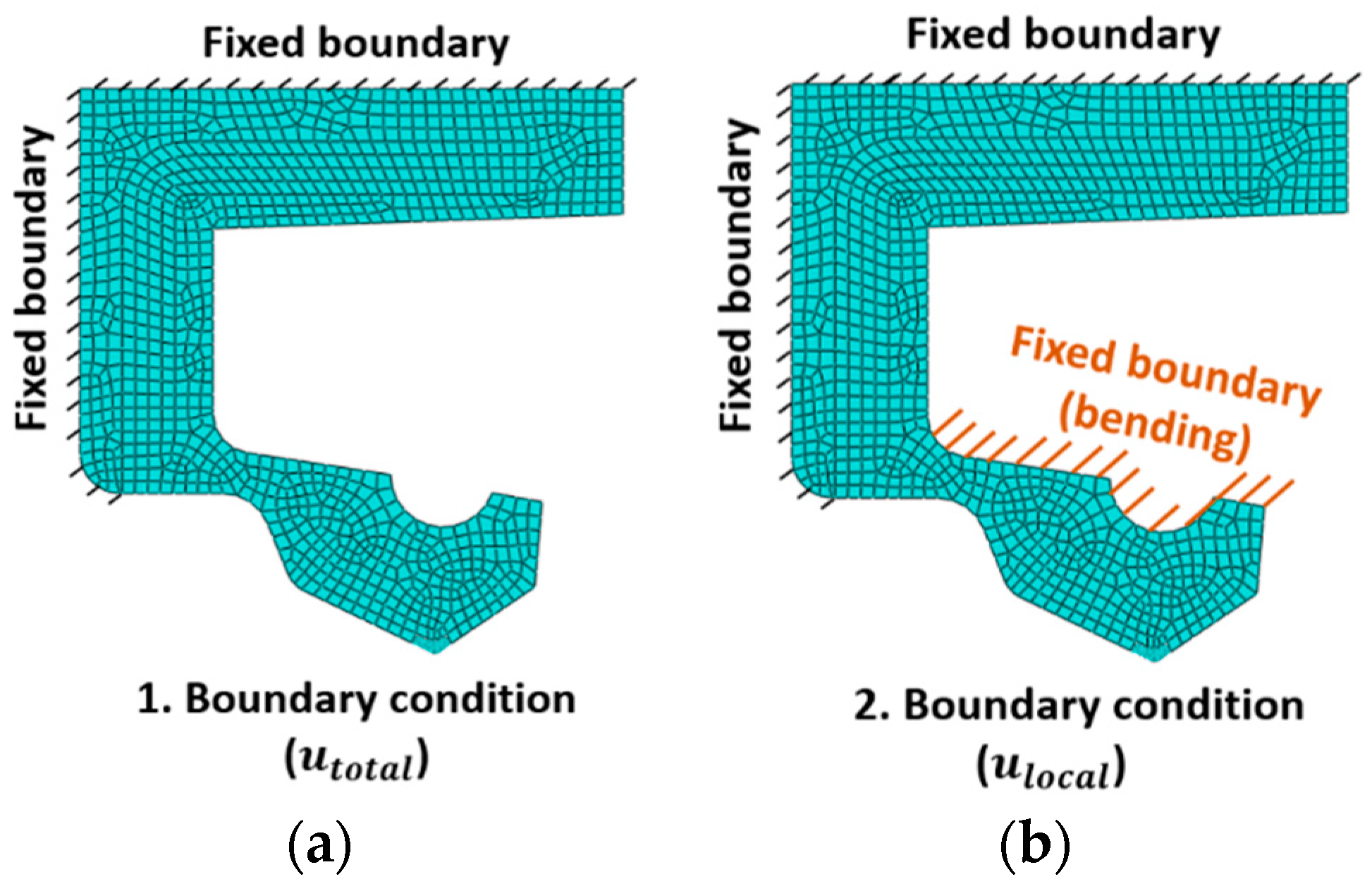
C i j k l x x ,…,   C i j k l x y ; S i j k l x x ,…,   S i j k l x y displacement influence coefficients of the local and structural deformations
p k l z ,   q k l x ,   q k l y ; u i j x ,   u i j y ,   u i j z Normal and tangential contact pressure; surface displacements
Γ c ,   Γ s l ,   Γ s t ;   s x ,   s y ;   δ x , δ y , δ z contact area, sliding zone, adhesion zone; sliding paths in x- and y- direction; body displacement in x-, y- and z- direction
wear parameters
α A , α F ; V , Δ h ;   e R ;   E d x , E d y Wear coefficient according to Archard, Fleischer; wear volume, wear increment height; friction energy density; friction work in x- and y- direction

References

  1. Foko, F.F.; Heimes, J.; Magyar, B.; Sauer, B. Reibenergiebasierte Verschleißsimulation für Radialwellendichtringe; Conference Paper; GfT-Tagung: Göttingen, Germany, 2019. [Google Scholar]
  2. Polonsky, I.A.; Keer, L.M. A numerical method for solving rough contact problems based on the multi-level multi-summation and conjugate gradient techniques. Wear 1999, 231, 206–219. [Google Scholar] [CrossRef]
  3. Magyar, B.; Sauer, B. Methods for the simulation of the pressure, stress, and temperature distribution in the contact of fractal generated rough surfaces. Proc. Inst. Mech. Eng. Part J J. Eng. Tribol. 2017, 231, 489–502. [Google Scholar] [CrossRef]
  4. Gallego, L.; Nelias, D.; Deyber, S. A fast and efficient contact algorithm for fretting problems applied to fretting modes I, II and III. Wear 2010, 268, 208–222. [Google Scholar] [CrossRef]
  5. Willner, K. Fully Coupled Frictional Contact Using Elastic Halfspace Theory. J. Tribol. 2008, 130, 1–8. [Google Scholar] [CrossRef]
  6. Jacq, C.; Nelias, D.; Lormand, G.; Girodin, D. Development of a Three-Dimensional Semi-Analytical Elastic-Plastic Contact Code. J. Tribol. 2002, 124, 653–667. [Google Scholar] [CrossRef]
  7. Yu, C.; Wang, Z.; Wang, Q.J. Analytical frequency response functions for contact of multilayered materials. Mech. Mater. 2014, 76, 102–120. [Google Scholar] [CrossRef]
  8. Wang, Z.; Jin, X.; Zhou, Q.; Ai, X.; Keer, L.M.; Wang, Q. An Efficient Numerical Method with a Parallel Computational Strategy for Solving Arbitrarily Shaped Inclusions in Elastoplastic Contact Problems. J. Tribol. 2013, 135, 1–12. [Google Scholar] [CrossRef] [Green Version]
  9. Wang, Z.J.; Wang, W.Z. Partial Slip Contact Analysis on Three-Dimensional Elastic Layered Half Space. J. Tribol. 2010, 132, 1–12. [Google Scholar] [CrossRef]
  10. Wang, Z.-J.; Wang, W.-Z.; Meng, F.-M.; Wang, J.-X. Fretting Contact Analysis on Three-Dimensional Elastic Layered Half Space. J. Tribol. 2010, 133, 1–8. [Google Scholar] [CrossRef]
  11. Johnson, K.L. Contact Mechanics; Cambridge University Press: Cambridge, UK, 1985. [Google Scholar]
  12. Gallego, L. Fretting et Usure des Contacts Mécaniques: Modélisation Numérique. Ph.D. Thesis, L’Institut National des Sciences Appliquées de Lyon, Villeurbanne, France, 2007. [Google Scholar]
  13. Schallamach, A. Friction and Abrasion of Rubber. Wear 1958, 1, 384–417. [Google Scholar] [CrossRef]
  14. Debler, C. Bestimmung und Vorhersage des Verschleißes für die Auslegung von Dichtungen. Ph.D. Thesis, Universität Hannover, Hannover, Germany, 2005. [Google Scholar]
  15. Hegadekatte, V.; Kurzenhäuser, S.; Huber, N.; Kraft, O. A predictive modelling scheme for wear in tribometers. Tribol. Int. 2008, 41, 1020–1031. [Google Scholar] [CrossRef] [Green Version]
  16. Békési, N.; Váradi, K. Wear simulation of a reciprocating seal by global remeshing. Period. Polytech. Mech. Eng. 2010, 54, 71–75. [Google Scholar] [CrossRef]
  17. Frölich, D. Strategien und Modelle zur Simulation des Betriebsverhaltens von Radialwellendichtringen. Ph.D. Thesis, Universität Kaiserslautern, Kaiserslautern, Germany, 2016. [Google Scholar]
  18. Jennewein, B. Integrierter Berechnungsansatz zur Prognose des Dynamischen Betriebsverhaltens von Radialwellendichtringen. Ph.D. Thesis, Universität Kaiserslautern, Kaiserslautern, Germany, 2016. [Google Scholar]
  19. Engelke, T. Einfluss der Elastomer-Schmierstoff-Kombination auf das Betriebsverhalten von Radialwellendichtringen. Ph.D. Thesis, Leibniz Universität Hannover, Hannover, Germany, 2011. [Google Scholar]
  20. Thielen, S. Entwicklung eines TEHD-Tribosimulationsmodells für Radialwellendichtringe. Ph.D. Thesis, Universität Kaiserslautern, Kaiserslautern, Germany, 2019. [Google Scholar]
  21. Gross, D.; Becker, W. Mechanik Elastischer Körper und Strukturen; Springer: Berlin/Heidelberg, Germany, 2002. [Google Scholar]
  22. Hauer, F. Die Elasto-Plastische Einglättung Rauer Oberflächen und ihr Einfluss auf die Reibung in der Umformtechnik. Ph.D. Thesis, Technischen Fakultät der Universität Erlangen-Nürnberg, Erlangen, Germany, 2014. [Google Scholar]
  23. Teixeira Alves, J.; Guingand, M.D.E.; Vaujany, J.P. Set of functions for the calculation of bending displacements for spiral bevel gear teeth. Mech. Mach. Theory 2010, 45, 349–363. [Google Scholar] [CrossRef]
  24. Teixeira Alves, J. Définition Analytique des Surfaces de Denture et Comportement Sous Charge des Engrenages Spiro-Coniques. Ph.D. Thesis, L’Institut National des Sciences Appliquées de Lyon, Villeurbanne, France, 2012. [Google Scholar]
  25. Archard, J.F. Wear theory and mechanisms. In Wear Control Handbook; Peterson, M.B., Winer, W.O., Eds.; ASME: New York, NY, USA, 1980. [Google Scholar]
  26. Fleischer, G. Energetische Methode zur Bestimmung des Verschleißes. Schmierungstechnik 1973, 4, 269–274. [Google Scholar]
  27. Kaiser, C. Entwicklung Einer Prüfmethodik für Modelluntersuchungen an Schmutzbeaufschlagten Radial-Wellendichtringen. Ph.D. Thesis, Universität Kaiserslautern, Kaiserslautern, Germany, 2016. [Google Scholar]
Figure 1. Radial shaft sealing rings (RSSR) tribological system.
Lubricants 08 00015 g001
Figure 2. Half-space under normal (Boussinesq problem) and tangential (Cerruti problem) single load at the origin.
Lubricants 08 00015 g002
Figure 3. Decomposition of the contact displacements at the sealing lip (a) local displacement component, (b) global displacement components from the structural bending.
Lubricants 08 00015 g003
Figure 4. Discretized half-space surface with a normal surface load.
Lubricants 08 00015 g004
Figure 5. Finite element (FE) model [17] to determine the structural influence matrices.
Lubricants 08 00015 g005
Figure 6. Boundary conditions for determining contact displacement, (a) the total displacement, (b) the local displacement.
Lubricants 08 00015 g006
Figure 7. (a) RSSR contact, (b) sealing lip, and shaft geometry in half-space contact model.
Lubricants 08 00015 g007
Figure 8. Comparison between the ideally smooth and the measured sealing lip profile for the RSSR made of FKM.
Lubricants 08 00015 g008
Figure 9. (a) Normal and tangential contact problem, (b) normal contact condition, (c) tangential contact condition.
Lubricants 08 00015 g009
Figure 10. The iterative solution of the frictional contact problem.
Lubricants 08 00015 g010
Figure 11. Experimental friction torque and speed stages of the combination polyacrylate rubber (ACM) and mineral oil.
Lubricants 08 00015 g011
Figure 12. Experimental friction torque characteristics of the six different elastomer–lubricant combinations.
Lubricants 08 00015 g012
Figure 13. (a) Comparison of contact pressure with finite element method (FEM) and half-space model, (b) influence of structural deformation on contact pressure and contact width.
Lubricants 08 00015 g013
Figure 14. Contact simulation results for the combination ACM–mineral oil. (a) First view to show the decrease of the contact pressure values with increasing wear (sliding distance), (b) second view showing the increasing of the contact width with increasing wear (sliding distance).
Lubricants 08 00015 g014
Figure 15. Comparison of the simulation results for the individual elastomer–lubricant combination. (a) ACM-lubricant combination, (b) FKM-lubricant combination, (c) NBR-lubricant combination.
Lubricants 08 00015 g015
Figure 16. Comparison of simulation and experimental results for the individual elastomer–lubricant combination. (a) wear volume, (b) contact width.
Lubricants 08 00015 g016
Figure 17. Comparison of the contact pressure simulated with the ideal smooth and measured sealing lip profile.
Lubricants 08 00015 g017
Figure 18. Simulated cumulative wear height after 100 km, 3000 km, and 5000 km sliding distance for the combination FKM–mineral oil.
Lubricants 08 00015 g018
Figure 19. (a) Simulated sealing lip profile changes after 100 km, 3000 km, and 5000 km sliding distance, for the combination FKM–mineral oil. (b) Comparison between experimental and simulated sealing lip profile after 5000 km sliding distance.
Lubricants 08 00015 g019
Table 1. Geometry and material parameters for simulation.
Contact Partner No.Radius (mm)Modulus of Elasticity (MPa)Poisson’s Ratio (-)
No.1(Shaft)402100.3
No.2 (ACM-Elastomer) 1.930.49
No.2 (FKM-Elastomer) 4.420.49
No.2 (NBR-Elastomer) 3.830.49
Table 2. Experimentally determined input variables for wear simulation.
Exp NoElastomer-Lubricant-Combination Radial   Force   F r a d   ( N )   at   the   Start   of   the   Experiment Radial   Force   F r a d   ( N )   at   the   End   of   the   Experiment Wear   Energy   Density   e R   ( Nmm / mm ³ )
1ACM-Mineral Oil19.02210.685.3445 × 1010
2ACM-PAO19.02212.334.9256 × 1010
3FKM-Mineral Oil12.7239.581.6791 × 1011
4FKM-PAO12.7239.271.4806 × 1011
5NBR-Mineral Oil18.5710.683.6394 × 1010
6NBR-PAO18.5711.931.4230 × 1011

