Assessment of Shaft Surface Structures on the Tribological Behavior of Journal Bearings by Physical and Virtual Simulation

Abstract

Optimizing the surface topography of cast iron crankshafts offers the opportunity to use this material as an alternative to steel in high-performance combustion engines. In the past, this was not possible due to the higher wear on bearing shells and the higher friction losses in relation to forged steel shafts. In order to find an optimized shaft micro topography, the friction and wear behavior of steel and cast iron shafts with different surface treatments were compared to each other, using a combined physical (experimental) and a virtual (computational) simulation approach. The experiments were carried out with a rotary tribometer using a journal bearing test configuration with the possibility to test real-life bearing shells and shaft specimens, manufactured from real-life crankshafts. In the experiments, a polished steel shaft with low bearing wear was effective. The optimization of cast iron crankshafts by a novel surface treatment showed a significant reduction of bearing wear in relation to the classical surface finishing procedures of cast iron shafts. A computational simulation approach, considering the real-life micro topography by using the Navier–Stokes equations for the calculation of micro hydrodynamics, supports the assessment of fluid friction. The virtual simulation shows, in accordance to the experimental results, only a minor influence of the investigated shaft topographies on the fluid friction. Further optimization of shaft surfaces for journal bearing systems seems possible only by the usage of patterned micro topographies.

1. Introduction

Hydrodynamic journal bearings are widely used machine elements, and due to their advantages, they are now standard bearings in internal combustion engines. The components of hydrodynamic journal bearings include exchangeable bearing shells, a rotating shaft, and an intermediate lubricant. Optimization of each component can reduce mixed or fluid friction losses, subsequently increasing the efficiency of modern combustion engines. Furthermore, an unstable increase of wear, also known as seizure or scuffing, on the one hand and mild wear during standard start/stop operation on the other hand need to be taken into account. A holistic approach to evaluating friction, seizure resistance, and lifetime limitation by mild start–stop wear is important for the design of components especially for highly loaded journal bearings, such as crankshaft bearings in internal combustion engines.

Crankshafts for high-performance combustion engines are usually made from forged steel to guarantee lifetime in terms of fatigue and bearing wear [1]. Surface finishing processes generate a topography that results in good tribological performance. Crankshafts from cast iron characteristically show problematic metal burrs near the graphite regions, generating higher wear on the bearing shells and poorer tribological performance [2]. Apart from these disadvantages, cast iron crankshafts offer potential for lightweight design and cost-efficient production. Strength levels have been increased and come near to those of forged crankshafts [3].

Optimization of cast iron shafts in crankshaft bearing systems can be supported by the use of a tribological simulation technique. The term simulation refers to physical simulation (experiment) as well as virtual simulation (computational calculation) [4,5]. Both techniques try to mimic the real tribological conditions in the application.

Physical simulation is done by laboratory test models (also defined as physical simulation models) with a wide band of measurement possibilities and input parameter settings. Fundamental model test systems [6] compete with application-near journal bearing rigs [7,8]. A compromise in terms of result transfer and efficiency can be achieved by using an application-near tribometer test methodology [9]. Test strategies, which define the test program, are adapted for the respective goal of research [10]. Examples can be found in [11] for research on the seizure resistance of journal bearing materials in engine applications and in [12] for the assessment of lifetime due to mild wear during start/stop operation.

Using a virtual simulation requires a virtual simulation model containing the components of the tribosystems with specific material and geometry parameters coupled with the boundary conditions at operation (speed, load, and temperature) by mathematical relations. Estimation of friction and mild wear behavior are subjects of implemented virtual simulations of journal bearings [13,14]. Macro models, using elasto-hydrodynamic relations, can be expanded with coupled micro models to take the effects of micro hydrodynamics and solid contact into account [15,16].

A micro model, for consideration of micro hydrodynamics, calculates the flow through the rough lubricating gap and is coupled by flow factors with the macro model. First described by Patir & Cheng [17,18], the micro model uses an approach based on the Reynolds equation, calculating a flow that is disturbed or supported by the roughness topography in relation to ideal smooth surfaces. Exactly this relation between the flow of rough and ideal smooth lubricating gaps is known as the flow factor and can be implemented into the macroscopic Reynolds equation. Improvements to the original method of Patir & Cheng were made, for example, by the implementation of real surface topographies, and no virtual generated ones, and the consideration of cavitation effects [19,20]. Using the Reynolds equation is recommended as long as the errors due to the derivation from the Navier–Stokes equations are small. This is the case for the most macroscopic journal bearing models as well as for micro models with substantially smooth roughness profiles and would be the case for the most common bearing and shaft surfaces [21,22]. The trend in the research towards patterned micro topographies calls for updated simulation strategies using the Navier–Stokes equations for solving the micro model. Based on the method of de Kraker [23,24], authors presented, in a previous publication, a novel approach for modeling surface topography effects in hydrodynamic lubrication [25].

The combination of physical and virtual simulation, and thus experimental and computational results, shows high potential for increasing our basic understanding of tribosystems [26,27]. Therefore, this combination can be used for the optimization of critical journal bearing systems, for example, the crankshaft bearings of automotive combustion engines.

To make use of casted crankshafts in high-performance engines possible, different surface treatments are compared in this article with the goal of comparing and understanding wear and friction properties under application-near conditions. This task is carried out by a physical simulation on a rotational tribometer together with a virtual simulation, using a novel approach for modeling surface topography effects in hydrodynamic lubrication [25]. Besides finding an optimization potential for crankshaft surface topographies, this study allows for comparison and validation between physical and virtual simulation approaches.

2. Materials and Surface Structures

For an application-near estimation of the influence of shaft structures, the components for the simulation were directly taken out from the production line considering different materials with different surface treatments and subsequently with different roughness parameters, given in

Table 1. Investigated shaft variants.

Short Name	Material	Surface Treatment	Sz [µm]	Spk [µm]	Svk [µm]	Phys. Sim.	Virt. Sim.
Steel 1	Steel	Classic polishing process	1.9	0.266	0.275	x	x
Steel 2	Steel	Grinding process	5.2	0.323	0.284	x
Cast Iron 1	Cast iron	Classic polishing process	2.9	0.364	0.345	x
Cast Iron 2	Cast iron	Novel Surface Treatment 1	3.2	0.230	0.210	x
Cast Iron 3	Cast iron	Novel Surface Treatment 2	2.3	0.175	0.189	x	x

. Based on an optical surface measurement ($400\times 800\mathsf{\mu }$m), according to ISO 25178 [28], we can show different maximum roughness heights Sz [29] for the collection of shaft variants. Furthermore, the reduced peak height Spk and the reduced valley depth Svk can give an impression of what the Abbott-curve and subsequently the distribution of peaks and valleys may look like. Microscopic images, which visualize the characteristic surface topographies, can be found in Section 5.3.

For the five shaft variants, listed in Table 1, a physical simulation was carried out with a focus on wear and friction assessment. A virtual simulation for closer research of the hydrodynamic properties of the micro topography was established for Steel 1 and the most potential alternative variant, Cast Iron 3.

For all experiments, the same polymeric bearing shells (IROX©, FEDERAL-MOGUL Glyco, Wiesbaden, Germany) and the same engine oil (Castrol EDGE Professional BMW LL 14 FE+ 0W-20, BP Europa SE, Hamburg, Germany) were used.

The FEDERAL-MOGUL IROX © is a high performance automotive crankshaft bearing shell, containing an aluminium-based lining material with a polymeric coating on top and an initial surface roughness of $Sz=6.8\mathsf{\mu }$m. SEM (scanning electron microscopy) and EDX (Energy dispersive X-ray spectroscopy) analysis shows intermetallic hard phases of Al–Ni, Al–Cu, and Al–Fe–Si–Mn and soft phases of Sn in the lining material (see Figure 1). The top coating contains boron nitride, potentially as solid lubrication, and further fillers for advanced running performance (e.g., iron oxide and silicon carbide) embedded in the polymeric matrix [30].

3. Physical Simulation Methodology

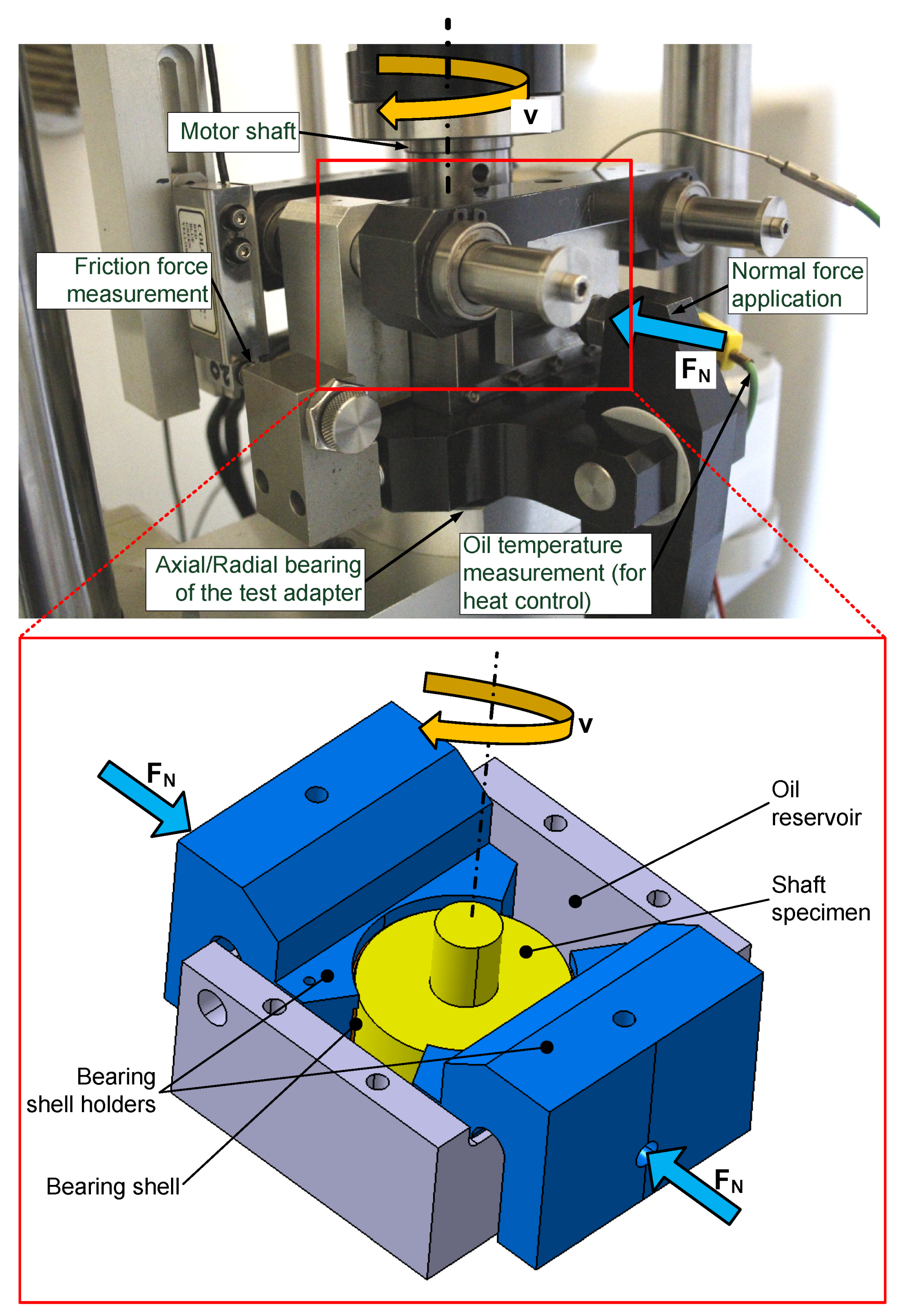
3.1. The Physical Simulation Model

The model for physical simulation of a crankshaft bearing of an internal combustion engine is implemented on a rotational tribometer TE92 of Phoenix Tribology (see Figure 2). The changeable shaft specimen (turning with speed v) is symmetric loaded by two journal bearing shells with a 120° contact angle using pneumatic air bellows applying the normal force $F_N$. The shaft specimens have a diameter of 50 mm and a width of $14.7$ mm. The relative bearing clearance is manufactured to 1.6 ‰, which results in a bearing diameter of ≈ 50.08 mm. The system sits in an open oil reservoir with an 80 mL lubricant volume, which can be heated by electrical resistance heating. To guarantee reproducible hydrodynamic conditions, the heat control uses a thermo couple, measuring the oil temperature in the reservoir (accuracy < 1 °K). The combination of free rotation of the bearing adapter, supported by a load cell on the main frame, enables a sensitive friction force measurement and subsequently a friction coefficient measurement with a relative error of $\approx 2.3\%$ (details can be found in [9]).

A pre- and post-test measurement of bearing shell weight and thickness is used for determining bearing wear. An exemplary procedure of thickness measurement of one bearing shell is shown in Figure 3. Reproducibility of the weight loss measurement was $\pm 0.02$ mg. For the thickness measurement, which uses a kind of outside micrometer, reproducibility was $\pm 0.5\mathsf{\mu }$m. The thickness loss measurement uses the maximum values per row averaged for one test (6 maximum values per test), named the averaged maximum wear height, to compare individual tests between each other. The gravimetrical measurement uses an average of the weight loss of both bearing shells per test.

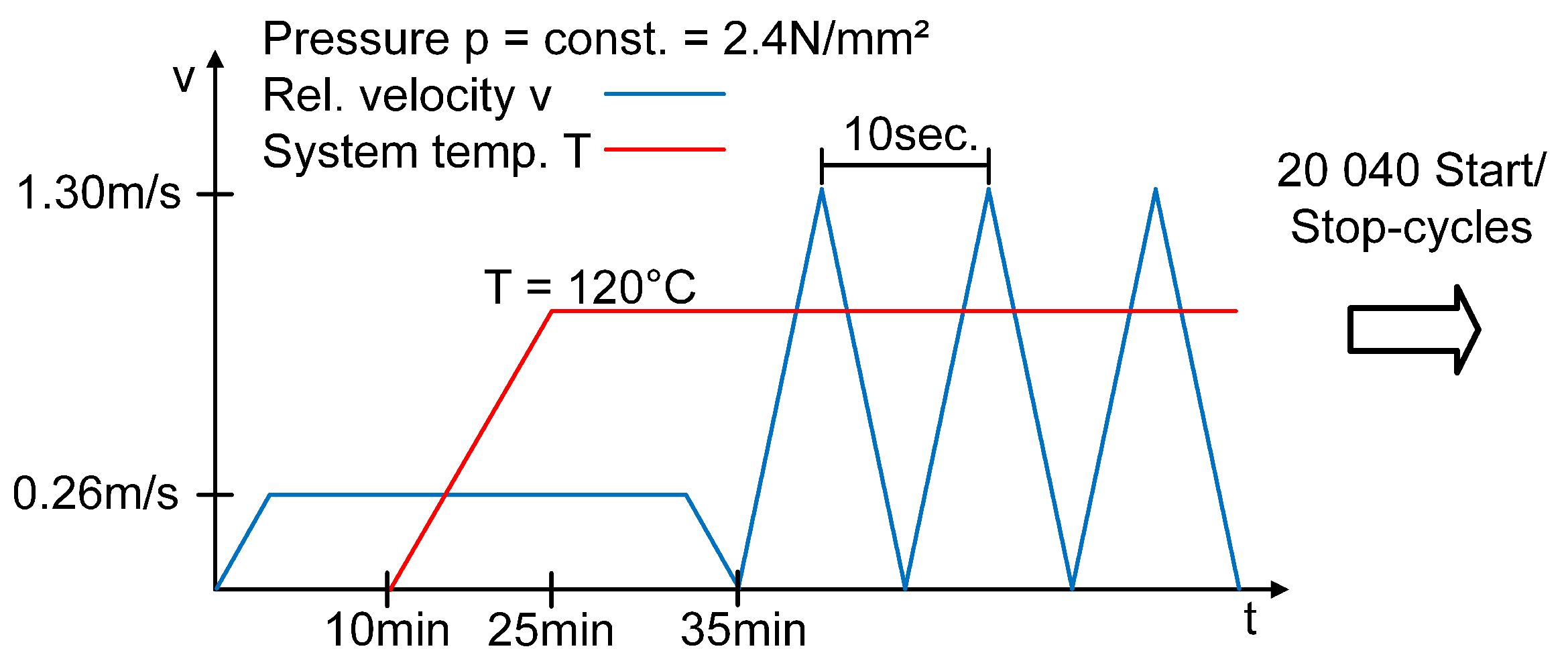
3.2. The Physical Simulation Strategy

For a ranking of the wear height and wear volume, as well as for the evolution of mixed and fluid friction, a start/stop test strategy with exactly 20,040 start/stop cycles is used (see Figure 4). A running-in of the system is achieved at a constant speed of 0.26 m/s, followed by a heating phase with a still standing shaft. The start/stop test procedure is carried out at a 120 °C oil temperature and a constant normal force to generate a pressure of 2.4 N/mm${}^2$ on the projected area. We performed two parallel tests per shaft variant.

For friction assessment, every 60th acceleration ramp is recorded by 1 kHz high speed data acquisition, resulting in 334 recorded Stribeck curves. An energy approach is used to compare the different shaft variants between each other. For the recorded Stribeck curves, frictional energy is separated into mixed friction and fluid friction (see Figure 5). Energy loss is then calculated for each friction regime by integrating the multiplication of coefficient of friction $\mu$ with the normal force $F_N$ and the relative velocity of the sliding partners v over time t:

$$E_{loss}^{Mixed}={\int }_0^{t_{minCOF}}\mu F_{N}vdt$$

(1)

$$E_{loss}^{Fluid}={\int }_{t_{minCOF}}^{t_{end}}\mu F_{N}vdt.$$

(2)

4. Virtual Simulation Methodology

4.1. The Virtual Simulation Model

The virtual simulation model is split into a macro model, containing the macroscopic geometry (shaft and bearing shells with specimen holders) and a micro model for considering the micro hydrodynamic behavior. Both are coupled via flow factors, so a change of the micro topography can affect the macroscopic bearing behavior. In the following, the most important information on the simulation models are given. Details can be found in [13] for the macro model and in [25] for the micro model.

The EHD macro model is implemented in COMSOL Multiphysics by an FEM-Mesh with around 43,000 elements and uses the original geometry of the shaft specimen and the bearing shells mounted in the bearing shell holders. The Reynolds Equation (3) is solved on the refined mesh of the bearing shell surface, using the thin-film-flow module of COMSOL Multiphysics. The gap height is directly calculated from the elastic deformable geometry of the contact partners. Oil temperature T, dynamic viscosity $\mathsf{\eta }$, and lubricant density $\mathsf{\rho }$ are held at constant values according to the experiment ($T=120{}^{\circ }\mathrm{C},\mathsf{\eta }=0.00548$ Pa·s,$\mathsf{\rho }=779.9$ kg/m${}^3$). Cavitation is considered by using the half-Sommerfeld boundary condition.

For the micro model, the CFD package OpenFOAM is used. On a finite-volume mesh of approximately 300,000 elements, which represents an area of the microscopic lubricating gap of $130\times 90\mathsf{\mu }$m, the Navier–Stokes equations are solved. The model contains the real-life shaft surface topography as well as the real-life shell topography, separated by the nominal lubricant gap height. According to the flow factor method, the model is completed by an inlet and outlet patch and by side faces with a symmetry boundary condition (no shear forces and no flow). A Newtonian viscosity model with a density-free viscosity of $\mathsf{\nu }=10$ mm${}^2$/s is used.

Real-life micro topographies are obtained via surface scanning by a focus-variation microscope. Via MATLAB, the received 3D-point cloud is smoothed with a 5th order Savitzky–Golay filter and aligned using a linear fit of the surface. Output of this post-routine was an STL surface mesh, which can be used for the SnappyHexMesh utility of OpenFOAM for generation of the micro model mesh.

4.2. The Virtual Simulation Strategy

Details on the solvers and the used approximation schemes, as well as the used convergence criteria can be found in the correlating methodical publications ([13] for the macro model and [25] for the micro model).

Patir & Cheng [17,18] presented an approach using the Reynolds equation for the flow calculation of the microscopic lubricating gap. Correlating the flow of the rough gap with a gap of the same nominal gap height but containing ideal smooth surfaces leads to flow factors. These factors, the pressure flow factor for a pressure-induced flow and the shear flow factor for a flow induced by the relative movement of the contact surfaces, are implemented in the macroscopic Reynolds equation, describing the overall bearing performance.

The calculation of the microscopic flow is a crucial part of this procedure. Patir & Cheng used the Reynolds equation for this purpose. However, the Reynolds equation is limited in its usage due to the derivation from the Navier–Stokes equations. A micro topography containing significant gradients in height, for example, patterned micro topographies, cannot be calculated properly by the Reynolds equation. The direct use of the Navier–Stokes equations is preferred.

Besides the different solution strategy of the micro model, implementation in the Reynolds equation of the macro model varies. The authors use an approach from de Kraker [23,24] for this coupling task that has been already used previously with virtual geometries [25]. The task in this article, to compute real-life surface topographies, is carried out with a similar procedure as published in [25], which is why only selected relations are written in this article.

Equation (3) depicts the macroscopic Reynolds equation used for the virtual simulation, whereby $h^{*}$ stands for the nominal lubricating gap height, $\eta$ for the dynamic viscosity, p for the pressure, and $U_1$ for the velocity of the moving surface. The counter surface, in this specific case the bearing surface, is considered with $U_2=0$. The pressure flow factors ${\chi }_p^x$/${\chi }_p^y$ and the shear flow factor ${\chi }_s^x$ are a function of the nominal lubricating gap height $h^{*}$ and taken as a constant over the x- and y -directions. Because of the major interest of this research in the fluid friction regime, a no pocket-squeeze effect, according to de Kraker [23], occurs, and the right side of Equation (3) can be set to zero. Furthermore, the flow correction factor ${\chi }_{sp}$ is set to 1, due to the relatively mild flow conditions. Based on previous research [25], no major influence of ${\chi }_{sp}$ is estimated.

$$-{\chi }_p^x\frac{\partial }{\partial x}\left(\frac{h^{*3}}{12\eta }\frac{\partial p}{\partial x}\right)-{\chi }_p^y\frac{\partial }{\partial y}\left(\frac{h^{*3}}{12\eta }\frac{\partial p}{\partial y}\right)+{\chi }_s^x\frac{U_1}{2}\frac{\partial h^{*}}{\partial x}+\frac{\partial h^{*}}{\partial t}=0.$$

(3)

The pressure flow factors ${\chi }_p^x$ and ${\chi }_p^y$ need to be separated into the individual direction of interest. For shear flow factor ${\chi }_s^x$, only the direction of movement, in this case the x-direction, is considered. The flow factors define the relation between the flow through the rough lubricant gap $Q_{p,rough}$/$Q_{s,rough}$ versus the flow through the ideal smooth lubricant gap $Q_{p,smooth}$/$Q_{s,smooth}$.

$${\chi }_p^x=\frac{Q_{p,rough}^x}{Q_{p,smooth}^x}$$

(4)

$${\chi }_p^y=\frac{Q_{p,rough}^y}{Q_{p,smooth}^y}$$

(5)

$${\chi }_s^x=\frac{Q_{s,rough}^x}{Q_{s,smooth}^x}.$$

(6)

Flow rates of the ideal smooth surfaces in Equations (5) and (6) $Q_{p,smooth}$ and $Q_{s,smooth}$ can be calculated in an analytical way:

$$Q_{p,smooth}=-\frac{h^{*3}}{12\nu }\frac{\Delta p}{\Delta x}b$$

(7)

$$Q_{s,smooth}=\frac{U_1{h}^{*}}{2}b$$

(8)

In these equations, $\Delta p$ is the applied pressure gradient for the pressure flow calculation $p_{Inlet}-p_{Outlet}$, $\Delta x$ is the distance between inlet and outlet, and b is the width of the micro model. The flow rate of the rough lubricating gap is the output of the CFD simulation and can be determined by Equation (9). It calculates the flow through a surface $A_{cross}$, which lies across the flow direction, using the velocity vectors $\mathbf{u}$ from the CFD calculation together with normal vectors $\mathbf{n}$ of $A_{cross}$. Separation into pressure and shear-induced flow is done by the boundary conditions of the CFD simulation.

$$Q_{rough}={\int }_{A_{cross}}\mathbf{u}·{\mathbf{n}}_{A_{cross}}\mathrm{dA}.$$

(9)

By solving the macroscopic Reynolds equation given in 3 on the bearing area A, it is possible to calculate the nominal gap height distribution $h^{*}$ by taking the force equilibrium between the resulting vector of the fluid film pressure ${\mathbf{F}}_{hyd}$ and the external normal force vector ${\mathbf{F}}_N$ into account. Because this article focuses on the hydrodynamic performance of different surface topographies, a solid contact model and the load carrying capacity of asperities are not considered. Assuming that only positive pressure can be load carrying (half-Sommerfeld boundary condition), the force equilibrium can be written as

$${\mathbf{F}}_N+{\mathbf{F}}_{hyd}=0$$

(10)

with the hydrodynamic force as the integrated fluid pressure times the normal vector of the surface A:

$$F_{hyd}={\int }_{A}p{\mathbf{n}}_{A}dA\mathrm{with}p>0.$$

(11)

Knowing pressure and height distribution of the lubricating gap, calculation of the friction force $F_{Fluidfriction}$ and thus the coefficient of friction $CO{F}_{Fluid}$ is possible. Friction force acts against the movement direction of the shaft and is the integrated shear force over the bearing surface A.

$$F_{Fluidfriction}={\int }_A\left(\eta \frac{U_1}{h^{*}}+\frac{\partial p}{\partial x}\frac{h}{2}\right)dA$$

(12)

$$CO{F}_{Fluid}=\frac{F_{Fluidfriction}}{|{\mathbf{F}}_N|}.$$

(13)

A comparison between the fluid friction properties of the shaft variants used for the virtual simulation, as well as to the experimental data from the physical simulation is possible in that way.

5. Results of the Physical Simulation

All shaft variants vary in frictional behavior, especially static friction, and in terms of bearing lifetime under start/stop operation. For a qualitative comparison, accumulated frictional energy and bearing wear after 20,040 start/stop cycles were considered.

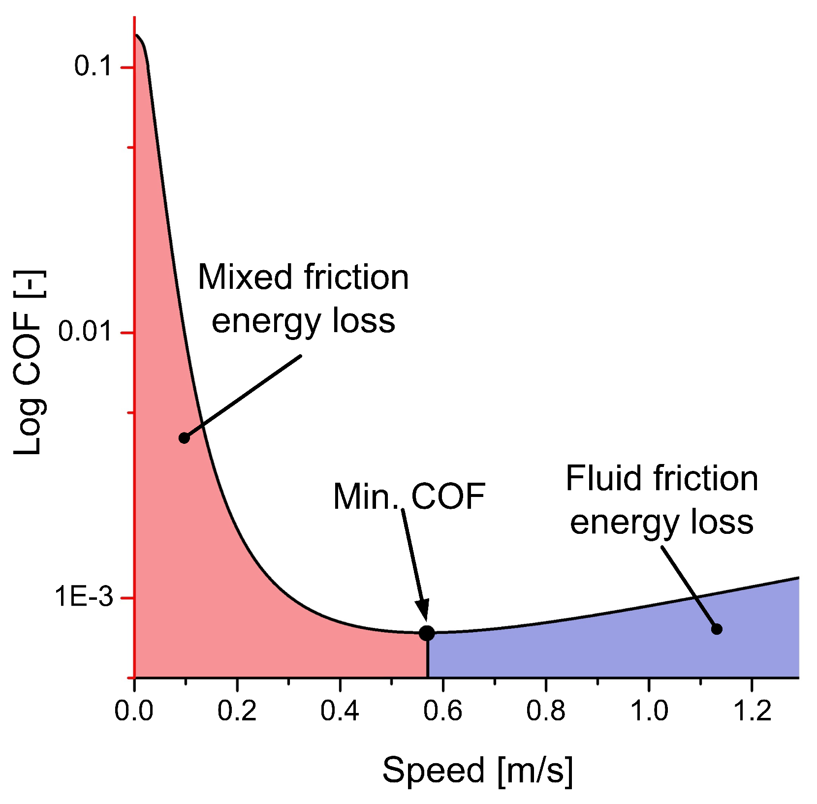
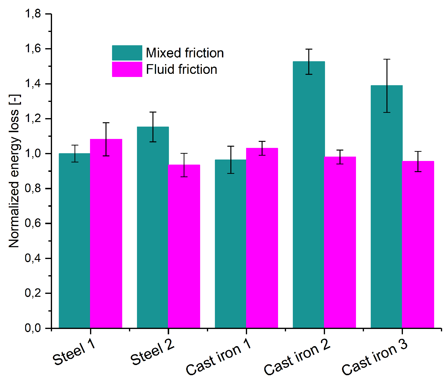
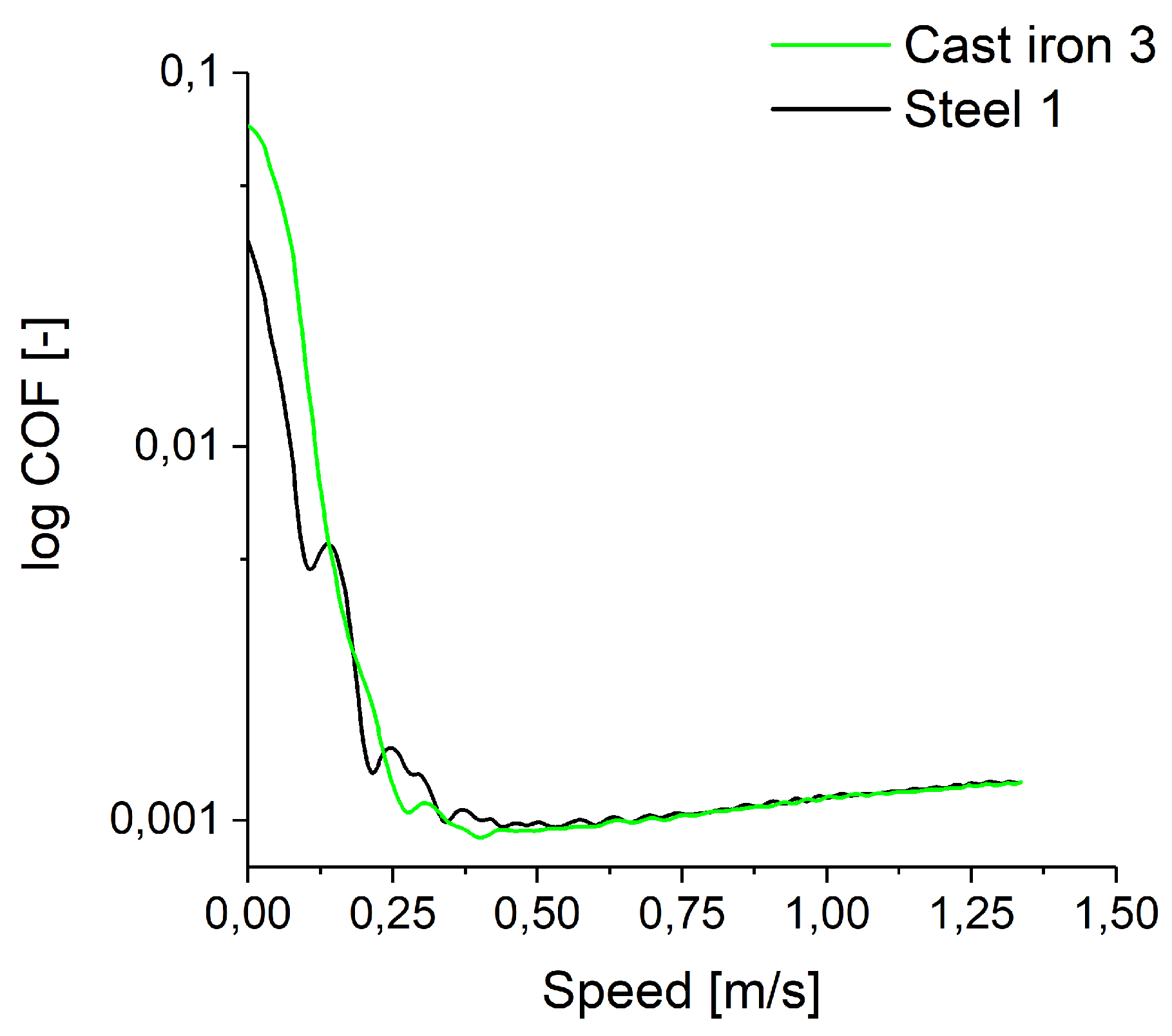
5.1. Friction Assessment

The continuous recording of friction data in the form of Stribeck curves allowed us to estimate both boundary and mixed friction, as well as the fluid friction regime. In Figure 6, the original Stribeck curves from a test with a Steel 1 shaft and a test with the Cast Iron 3 shaft are plotted, both taken after 20,040 start/stop cycles. In the fluid friction regime, both variants perform similarly. It should be recognized that COF is plotted on a logarithmic scale to visualize the fluid friction regime more clearly. Differences between these two curves can be detected in the form of a lower static friction for the steel shaft. Vibrations of the friction torque signal due to imperfections of alignment and the fast speed ramp have an impact on the COF curves in Figure 6.

For a wider view of the impact of the shaft surface topography on the friction behavior, an energetic approach, described in Section 3.2, was used. The accumulated friction energies for mixed and fluid friction (averaged over parallel tests and normalized with the mixed friction losses of Steel 1) are given in Figure 7.

Cast Iron 2 and Cast Iron 3 shafts show significant higher friction losses in the mixed friction regime compared to the steel shafts and the Cast Iron 1 shaft. In the fluid friction regime, no significant influence of the shaft surface topography is detectable.

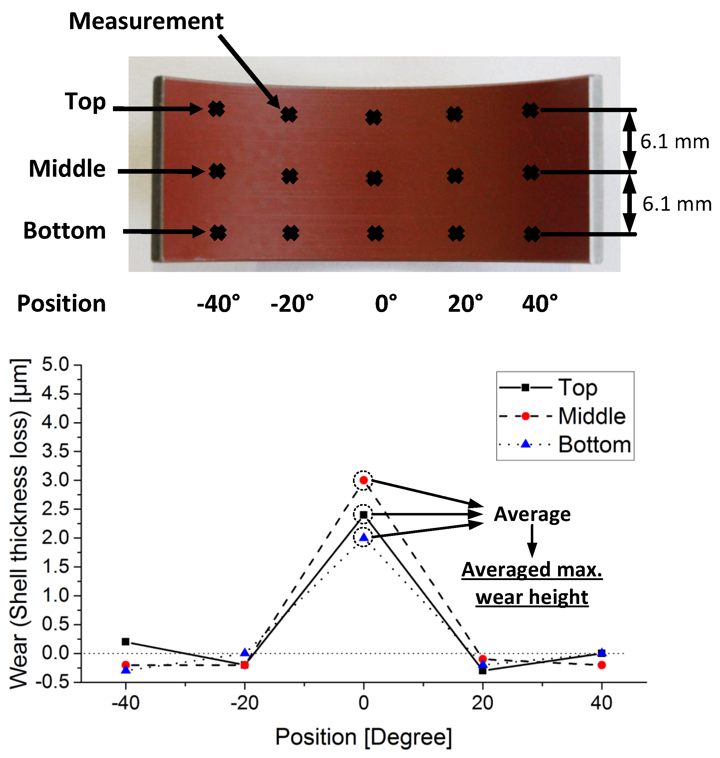
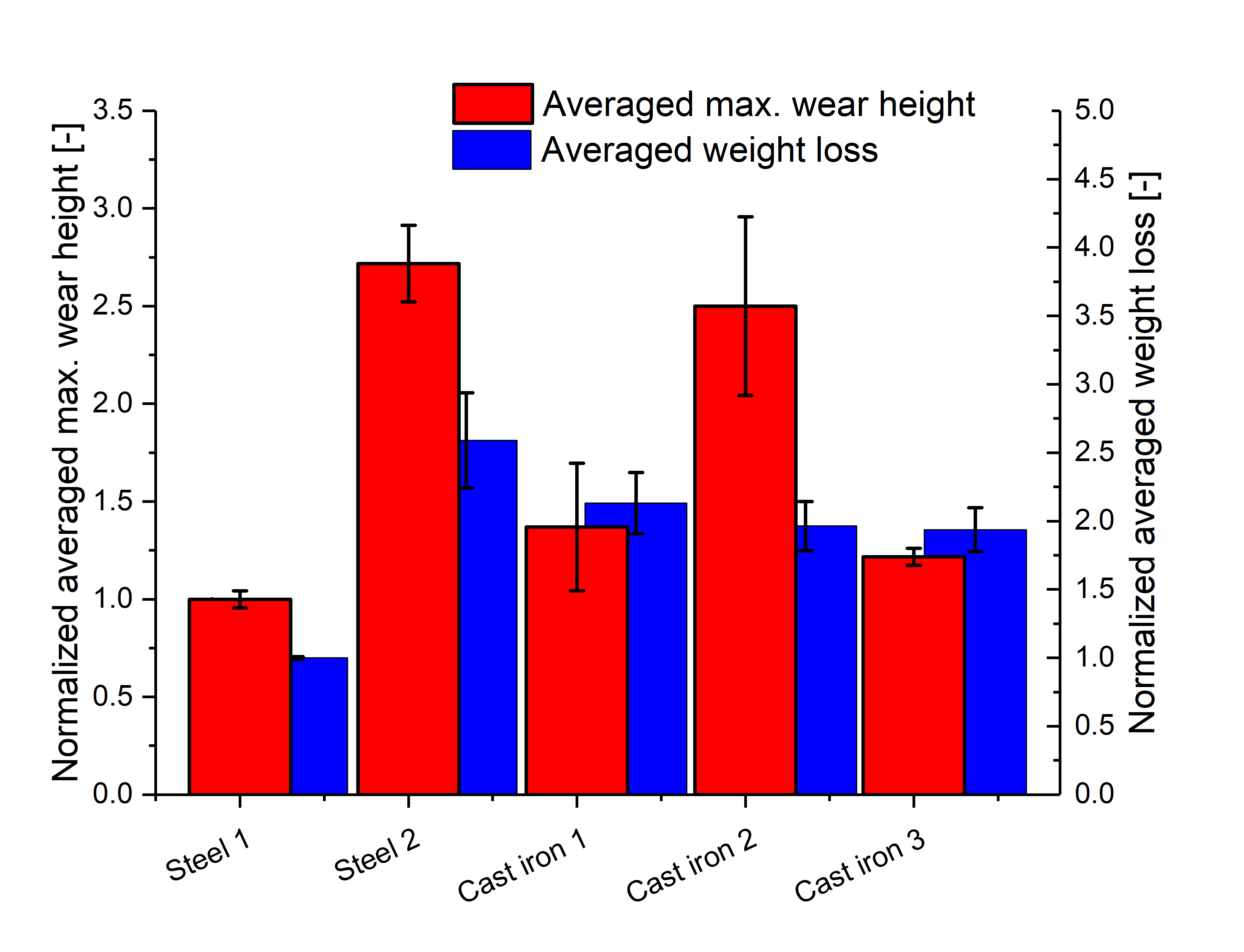
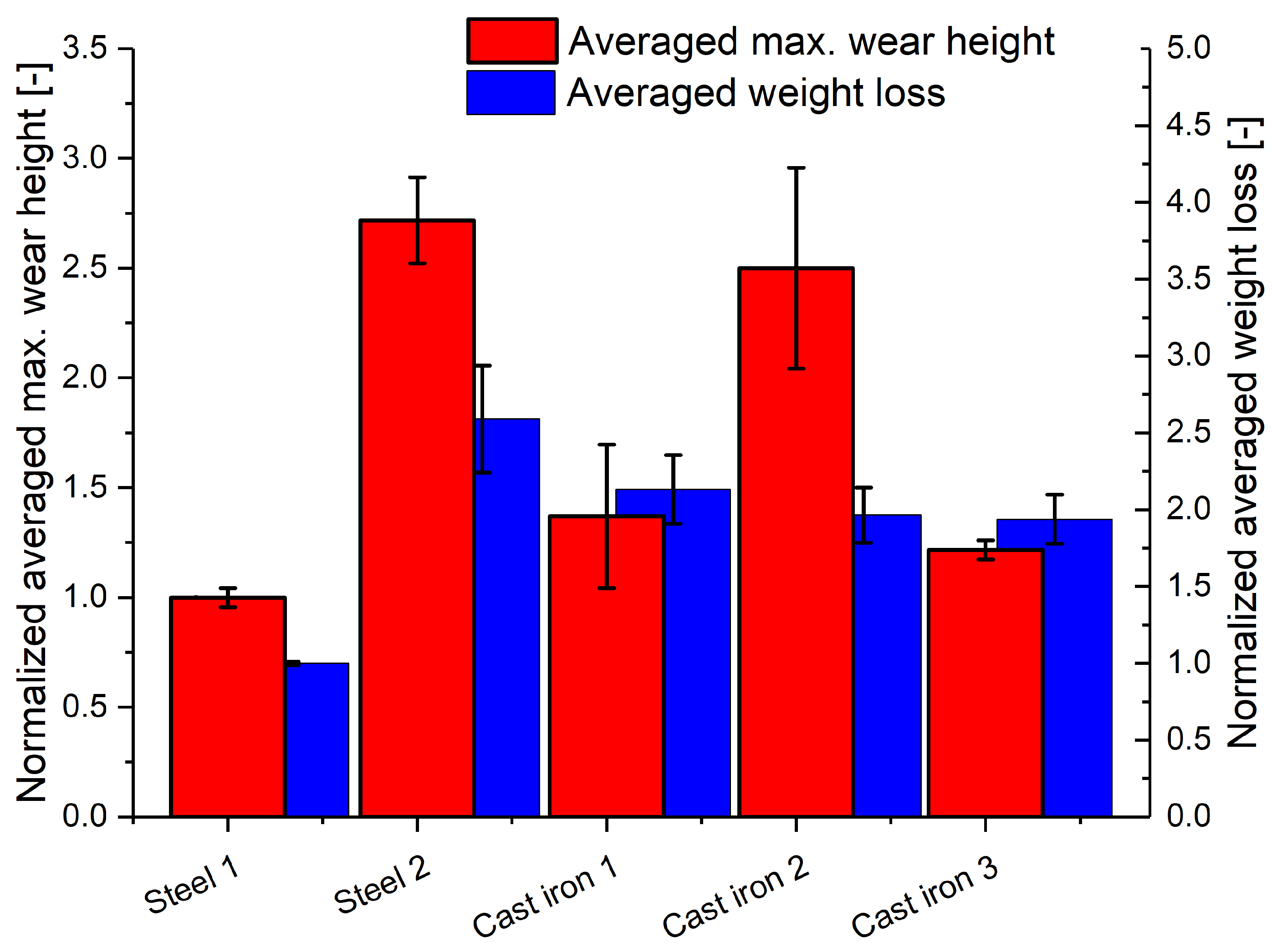
5.2. Lifetime Assessment

Via measurement of weight and thickness loss of the bearing shells, a wear ranking of the different shaft variants could be generated. In Figure 8, the values of the averaged maximum wear height (see Section 3.1) together with the weight loss of the bearing shells are plotted for each shaft variant, averaged over the parallel tests and normalized with the wear results of the Steel 1 shaft. The results of the thickness losses demonstrate the good performance of the classical polished steel and cast iron shafts as well as the cast iron shaft with Novel Surface Treatment 2 in comparison to the high wear height values of the ground steel shaft and the Cast Iron 2 shaft. This ranking is also seen for the gravimetric wear results. Only for Cast Iron 1 and 2 is a changing wear relation observed, which can be attributed to slight geometrical differences in the worn volume. Another important observation is that no shaft variant was able to remove the top coating of the bearing material (coating thickness is around 8–12 $\mathsf{\mu }$m) within 20,040 start/stop cycles, which visualizes the excellent sliding performance of optimized polymeric bearing materials.

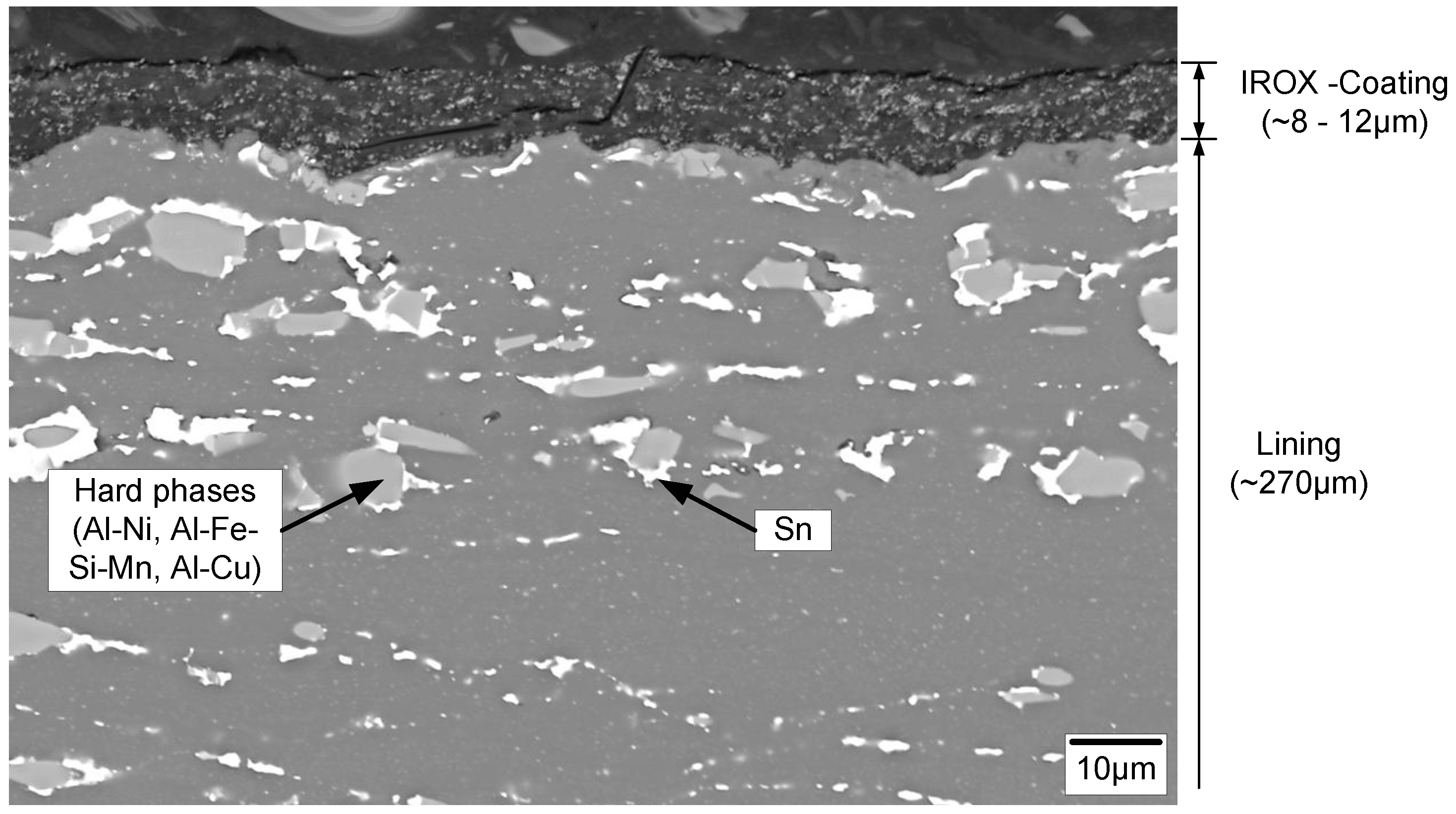
5.3. Surface Analysis and Tribo Mechanisms

Friction and wear results indicate an influence of the shaft material and the finishing process on the tribological performance of journal bearings. In order to understand the mechanism behind the observed behavior, surface analysis was carried out. Figure 9 depicts a summary of pre- and post-test SEM images as well as hypotheses for the tribo mechanism taking place. All findings regarding topography changes were additionally confirmed by an Alicona InfiniteFocus 3D confocal microscope.

On the Steel 1 shaft, a fine structured surface with polishing grooves in the running direction is visible. After the test run with 20,040 start/stop cycles, no major changes were observed on the shaft surface, except the formation of tribo layers containing O, Ca, and Zn (Steel 1 in Figure 9 and EDX 1 in

Table 2. EDX elemental analysis taken at 7.5 kV (values in atomic-%).

Location	C	O	Si	P	S	Ca	Fe	Zn
EDX 1	13.3	35.6	-	-	-	11.1	38.7	1.2
EDX 2	11.4	30.6	-	1.2	1.7	9.0	44.5	1.6
EDX 3	15.3	51.3	-	-	-	15.8	17.6	-
EDX 4	12.3	37.3	1.6	-	-	12.1	36.2	0.8
EDX 5	13.0	33.0	2.1	-	-	11.2	40.1	0.7

). The smooth surface results in low bearing wear and low frictional losses.

The Steel 2 shaft, which shows high bearing wear and moderate mixed friction, offers a surface topography with higher roughness. The initial as well as the surface after 20,040 start/stop cycles show grinding grooves in the running direction. Besides the formation of tribo layers, a slight smoothing of roughness peaks can be observed (Steel 2 in Figure 9 and EDX 2 in Table 2).

All cast iron shaft variants show for the initial state, as well as after testing, exposed graphite and differ only in the shape of the graphite-surrounding metal burrs. For the classical polished cast iron shaft (Cast Iron 1), the metal burrs were removed or pushed into the graphite during operation. A smooth surface with covering Ca tribolayers was generated. This explains the moderate bearing wear and the low mixed friction losses.

In contrast, the cast iron shaft with Novel Surface Treatment 1 (Cast Iron 2) shows sharp, compact edges around the graphite areas with no significant changes, due to the smoothing or flattening of these burrs during operation. Scratching of the uprising burrs generated poor performance for both aspects, the bearing wear and the frictional losses in the mixed friction regime.

Novel Surface Treatment 2 produces a surface topography given in Figure 9 under Cast Iron 3. The metal burrs were transferred into round elevations. The elevated structure contacts the counterpart and seems to be responsible for the high friction losses in the mixed friction regime. However, there is low bearing wear, which can be attributed to the round surface topography of the elevations. During tribological operation, the elevations are smoothed, and covering Ca-based tribolayers are formed.

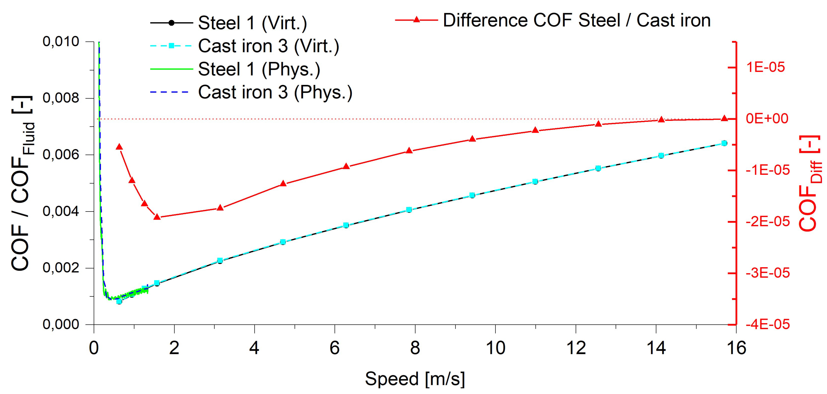
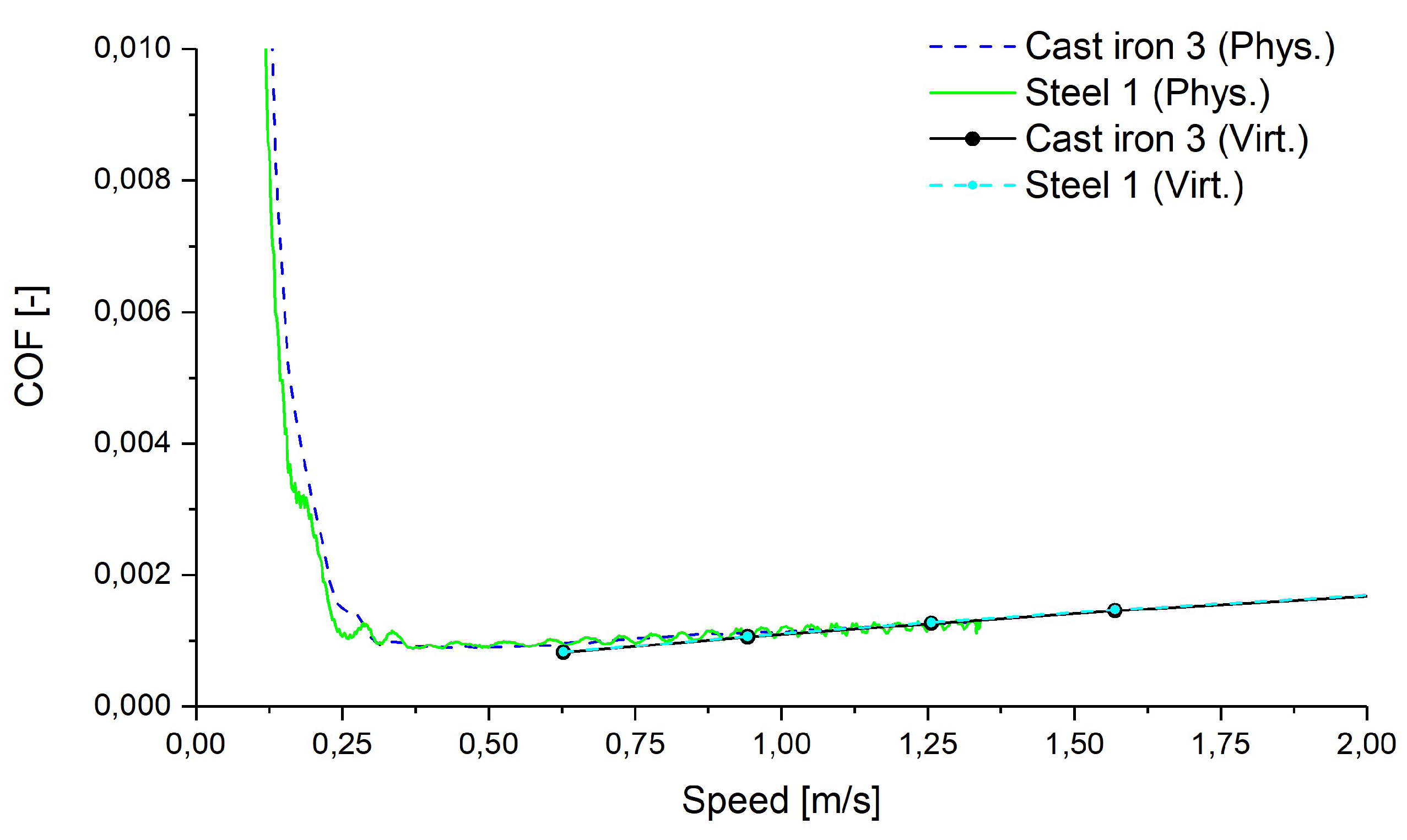
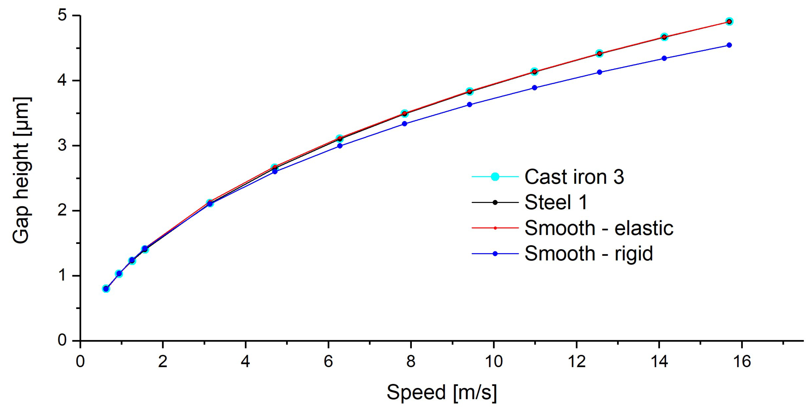
6. Results of the Virtual Simulation

For the two shaft variants with the lowest wear (Steel 1 and Cast Iron 3), a virtual simulation focusing on the hydrodynamics of the micro topography was conducted. Both shaft surfaces were paired with the same bearing shell topography to build the lubricating gap model. For the comparison, pressure flow factors in and perpendicular to the running direction were calculated, plotted in Figure 10 as a function of nominal gap height. It should be recognized that first contact between roughness peaks in the micro model occur at a nominal gap height of $0.7\mathsf{\mu }$m for Cast Iron 3 and $0.5\mathsf{\mu }$m for Steel 1.

Steel 1 shaft shows an increasing flow factor in the running direction and a decreasing flow factor perpendicular to the running direction. This can be interpreted as indicating that the flow through the rough gap is larger than that through an ideal gap with the same nominal gap height, in the case of the running direction. Flow perpendicular to the running direction is hindered by asperities and the flow appears to be less than that through an ideal smooth gap with the same nominal gap height.

For Cast Iron 3, the flow shows a decrease in both directions, in and perpendicular to the running direction. The graphite dimple in the center of the calculation area seems to generate isotropic micro hydrodynamic behavior. A hypothesis for the flow-increasing behavior in the range of $2\mathsf{\mu }$m would be the primary influence of the flow-increasing area at the graphite dimple (flow increases with h${}^3$). For gap heights below $2\mathsf{\mu }$m, the decreasing gap height beside the dimple reduces the overall flow and generates a flow-decreasing behavior of the surface. Nevertheless, the flow factors of both surface variants, Steel 1 and Cast Iron 3, are only of small dimensions, so that no significant impact on the macroscopic hydrodynamic performance could be expected. The time-consuming calculation of shear flow factors was therefore neglected.

Using the elasto-hydrodynamic macro model of the bearing shell holder and the shaft specimen, a consideration of the received flow factors on the macroscopic friction performance could be conducted. Due to the fact that, for this research, the hydrodynamic properties of the micro topography are of interest, only the fluid friction regime is taken into account. Shear flow factors, as well as a temperature-dependent oil viscosity, are neglected for this basic investigation on the behavior of flow factors (see Section 4.2). Cavitation for the macro model is considered to be in a half-Sommerfeld condition. The results of the COF due to fluid friction force over the relative velocity are plotted in Figure 11 (Steel 1 (Virt.) and Cast Iron 3 (Virt.)) using the flow factors from Figure 10, together with the COF results of the experimental investigations (Figure 11; Steel 1 (Phys.) and Cast Iron 3 (Phys.)). In addition, the difference in the calculated COF between the Steel 1 shaft and the Cast Iron 3 shaft $CO{F}_{Diff}=CO{F}_{Steel1(Virt.)}-CO{F}_{Castiron3(Virt.)}$ is given (Figure 11; Difference COF Steel/Cast Iron). The calculation of $CO{F}_{fluid}$ is performed down to a relative velocity of 0.6 m/s, where both surface variants are still separated by a lubricant gap.

There appears to be no significant difference between the experimental and calculated COF results. However, the simulation results match the experimental data quite well, at a speed above 0.6 m/s. $CO{F}_{Diff}$ shows a slightly lower COF for the steel shaft in the fluid friction regime. The virtual simulations were carried out up to a speed of 16 m/s, to show that both surfaces result in a similar fluid friction force, due to the increasing gap height and the decreasing influence of flow factors.

Details on the overlapping results of physical and virtual simulation can be found in Figure 12. For both surfaces variants, the results match within the spread of the experimental data.

The calculated gap heights (see Figure 13) indicate that the difference between Steel 1 and Cast Iron 3 is marginal. Comparing the two surfaces with an ideal smooth surface yields only minimal differences (a gap height of an elasto-hydrodynamic model with a smooth surface in Figure 13, “Smooth - elastic”). Regarding the neglecting of elastic deformations, as shown in Figure 13, “Smooth - rigid” plays a much greater role in the hydrodynamic performance. Especially in the area of higher relative speeds, this results in an underestimation of the gap height. This additional result should indicate the qualitative influence of surface topographies and flow factors on the results of a hydrodynamic calculation, which is marginal in relation to the consideration of elastic deformations.

Both the coefficient of friction based on fluid friction force and the lubricating gap height indicate only a minor impact of the surface topography. Moreover, with the inclusion of shear flow factors, no major impact of the micro hydrodynamics can be estimated, based on the already poor difference between the two shaft variants.

7. Conclusions and Outlook

The presented methodology of a physical simulation for the comparison of shaft topographies indicates significant differences in terms of bearing wear and friction losses. A novel approach for the virtual simulation of micro hydrodynamics shows similar results to those of the physical experiments and provides additional input on the understanding of tribological phenomena. While the possibilities of a combination of these two simulation approaches for research on tribosystems are shown, the main purpose of this article consists in the results of the optimization of cast iron shafts.

Using a smooth shaft surface topography, as can be found for the classical polished steel shaft, shows the best performance in terms of friction losses as well as for the mild wear of bearing shells. Surfaces with higher roughness, e.g., for the ground steel shaft, or inhomogeneous surface topographies, e.g., for the cast iron shafts, cannot achieve the tribological performance of a polished steel shaft. Optimizations of cast iron shafts by flattening the metal burrs around the graphite dimples can reduce the wear but leads to higher friction losses in the mixed friction regime. Virtual simulation could not confirm any potential major influence of the micro hydrodynamics. Comparing the effects of the micro hydrodynamics of the polished steel shaft with the novelly treated cast iron shaft reveals differences in the flow behavior, but overall any influence of micro hydrodynamics is negligible.

Following the fact that state-of-the-art finishing procedures generate surface topographies with subordinate micro hydrodynamic effects, only can a potential patterned micro topography of a bearing shaft show a major impact. Research in the field of patterned micro topographies, using physical and virtual simulation, could help to optimize journal bearings in terms of reducing bearing wear and friction losses.

For future research on this topic, it is planned to further improve both the physical and the virtual simulation methodology. The design process of future patterned micro topographies with a prospect for greater friction reduction can justify the implementation of more complex techniques in virtual simulations, such as shear flow factors or more complex cavitation models.

References

1. Kniewallner, L. Kurbelwellen. In Handbuch Verbrennungsmotor; Vieweg+Teubner: Berlin, Germany, 2010; Volume 5. [Google Scholar]
2. Summer, F.; Grün, F.; Schiffer, J.; Gódor, I.; Papadimitriou, I. Tribological study of crankshaft bearing systems: Comparison of forged steel and cast iron counterparts under start–stop operation. Wear 2015, 338–339, 232–241. [Google Scholar] [CrossRef]
3. Menk, W.; Kniewallner, L.; Prukner, S. Cast crankshafts as an alternative to forged crankshafts. MTZ Worldw. 2007, 68, 23–24. [Google Scholar] [CrossRef]
4. Bhushan, B. (Ed.) Modern Tribology Handbook; CRC Press LLC: Boca Raton, FL, USA, 2001. [Google Scholar]
5. Czichos, H. Tribologie-Handbuch: Tribometrie, Tribomaterialien, Tribotechnik, 3rd ed.; Springer Fachmedien: Wiesbaden, Germany, 2010. [Google Scholar]
6. Feyzullahoğlu, E.; Şakiroğlu, N. The wear of aluminium-based journal bearing materials under lubrication. Mater. Des. 2010, 31, 2532–2539. [Google Scholar] [CrossRef]
7. Hagemann, T.; Pfeiffer, P.; Schwarze, H. Measured and Predicted Operating Characteristics of a Tilting-Pad Journal Bearing with Jacking-Oil Device at Hydrostatic, Hybrid, and Hydrodynamic Operation. Lubricants 2018, 6, 81. [Google Scholar] [CrossRef] [Green Version]
8. Vlădescu, S.C.; Fowell, M.; Mattsson, L.; Reddyhoff, T. The effects of laser surface texture applied to internal combustion engine journal bearing shells—An experimental study. Tribol. Int. 2019, 134, 317–327. [Google Scholar] [CrossRef]
9. Summer, F.; Bergmann, P.; Grün, F. Damage Equivalent Test Methodologies as Design Elements for Journal Bearing Systems. Lubricants 2017, 5, 47. [Google Scholar] [CrossRef] [Green Version]
10. Grün, F.; Gódor, I.; Trausmuth, A.; Krampl, H. Damage oriented tribological model testing for internal combustion engines—Design of laboratory test strategies. Tribol. Schmier. 2013, 60, 5–12. [Google Scholar]
11. Summer, F.; Grün, F.; Offenbecher, M.; Taylor, S. Challenges of friction reduction of engine plain bearings—Tackling the problem with novel bearing materials. Tribol. Int. 2018, 131, 238–250. [Google Scholar] [CrossRef]
12. Summer, F.; Grün, F.; Offenbecher, M.; Taylor, S.; Lainé, E. Tribology of journal bearings: Start stop operation as life-time factor. Tribol. Und Schmier. 2017, 64, 44–54. [Google Scholar]
13. Bergmann, P.; Grün, F.; Gódor, I.; Stadler, G.; Maier-Kiener, V. On the modelling of mixed lubrication of conformal contacts. Tribol. Int. 2018, 125, 220–236. [Google Scholar] [CrossRef]
14. Bergmann, P.; Grün, F.; Summer, F.; Gódor, I. Evaluation of Wear Phenomena of Journal Bearings by Close to Component Testing and Application of a Numerical Wear Assessment. Lubricants 2018, 6, 65. [Google Scholar] [CrossRef] [Green Version]
15. Chengwei, W.; Zheng, L. An Average Reynolds Equation for Partial Film Lubrication With a Contact Factor. J. Tribol. 1989, 111, 188–191. [Google Scholar]
16. Dobrica, M.B.; Fillon, M.; Maspeyrot, P. Influence of Mixed-Lubrication and Rough Elastic-Plastic Contact on the Performance of Small Fluid Film Bearings. Tribol. Trans. 2008, 51, 699–717. [Google Scholar] [CrossRef]
17. Patir, N.; Cheng, H.S. An Average Flow Model for Determining Effects of Three-Dimensional Roughness on Partial Hydrodynamic Lubrication. J. Lubr. Technol. 1978, 100, 12–17. [Google Scholar] [CrossRef]
18. Patir, N.; Cheng, H.S. Application of Average Flow Model to Lubrication Between Rough Sliding Surfaces. J. Lubr. Technol. 1979, 101, 220–229. [Google Scholar] [CrossRef]
19. Meng, F.M.; Cen, S.Q.; Hu, Y.Z.; Wang, H. On elastic deformation, inter-asperity cavitation and lubricant thermal effects on flow factors. Tribol. Int. 2009, 42, 260–274. [Google Scholar] [CrossRef]
20. Dobrica, M.B.; Fillon, M.; Pascovici, M.D.; Cicone, T. Optimizing surface texture for hydrodynamic lubricated contacts using a mass-conserving numerical approach. Proc. Inst. Mech. Eng. Part J J. Eng. Tribol. 2010, 224, 737–750. [Google Scholar] [CrossRef]
21. Dobrica, M.B.; Fillon, M. About the validity of Reynolds equation and inertia effects in textured sliders of infinite width. Proc. Inst. Mech. Eng. Part J J. Eng. Tribol. 2009, 223, 69–78. [Google Scholar] [CrossRef]
22. Sahlin, F.; Larsson, R.; Marklund, P.; Almqvist, A.; Lugt, P.M. A mixed lubrication model incorporating measured surface topography. Part 2: Roughness treatment, model validation, and simulation. Proc. Inst. Mech. Eng. Part J J. Eng. Tribol. 2009, 224, 353–365. [Google Scholar] [CrossRef]
23. De Kraker, A.; van Ostayen, R.A.J.; van Beek, A.; Rixen, D.J. A Multiscale Method Modeling Surface Texture Effects. J. Tribol. 2007, 29, 221–230. [Google Scholar] [CrossRef]
24. De Kraker, A.; van Ostayen, R.A.J.; Rixen, D.J. Development of a texture averaged Reynolds equation. Tribol. Int. 2010, 43, 2100–2109. [Google Scholar] [CrossRef]
25. Pusterhofer, M.; Bergmann, P.; Summer, F.; Grün, F.; Brand, C. A Novel Approach for Modeling Surface Effects in Hydrodynamic Lubrication. Lubricants 2018, 6, 27. [Google Scholar] [CrossRef] [Green Version]
26. Prölß, M.; Schwarze, H.; Hagemann, T.; Zemella, P.; Winking, P. Theoretical and Experimental Investigations on Transient Run-Up Procedures of Journal Bearings Including Mixed Friction Conditions. Lubricants 2018, 6, 105. [Google Scholar] [CrossRef] [Green Version]
27. Varela, A.C.; Santos, I.F. Dynamic Coefficients of a tilitng pad with active lubrication: Comparison between theoretical and experimental results. J. Tribol. 2015, 137, 1–10. [Google Scholar]
28. ÖNORM EN ISO 25178-2:2012. Geometrical Product Specifications (GPS) ― Surface Texture: Areal Part 2: Terms, Definitions and Surface Texture Parameters; ISO: Geneva, Switzerland, 1996. [Google Scholar]
29. KEYENCE. Introduction to Roughness: Solving the Question about Profile and Surface Roughness Measurements. 2019. Available online: https://www.keyence.eu/ss/products/microscope/roughness/index.jsp (accessed on 15 January 2020).
30. Adam, A.; Prefot, M.; Wilhelm, M. Crankshaft bearings for engines with start-stop systems. MTZ Worldw. 2010, 71, 22–25. [Google Scholar] [CrossRef]
Figure 1. Microsection of the used bearing shell.
Lubricants 08 00008 g001
Figure 2. Set up of the test rig.
Lubricants 08 00008 g002
Figure 3. Thickness measurement methodology and an exemplary data graph.
Lubricants 08 00008 g003
Figure 4. Test strategy for the lifetime and friction assessment.
Lubricants 08 00008 g004
Figure 5. Schematic Stribeck curve with a separation of energy losses.
Lubricants 08 00008 g005
Figure 6. Stribeck curves of the Steel 1 shaft and the Cast Iron 3 shaft after 20,040 start/stop cycles.
Lubricants 08 00008 g006
Figure 7. Normalized frictional energy loss for 20,040 start/stops separated into mixed and fluid friction regimes.
Lubricants 08 00008 g007
Figure 8. Normalized averaged maximum bearing shell thickness loss for 20,040 start/stops.
Lubricants 08 00008 g008
Figure 9. Tribo mechanisms.
Lubricants 08 00008 g009
Figure 10. Calculated pressure flow factors.
Lubricants 08 00008 g010
Figure 11. Coefficient of fluid friction force, lubrication gap height, and difference in the COF between the two shaft variants over the relative velocity.
Lubricants 08 00008 g011
Figure 12. Detail on the COF comparison between the virtual model and the physical experiment.
Lubricants 08 00008 g012
Figure 13. Calculated gap heights for the steel and the cast iron surface, as well as for a smooth surface with elastic deformations and a smooth surface with rigid geometry.
Lubricants 08 00008 g013