Article

Numerical Simulation of a Slipper Model with Multi-Lands and Grooves for Hydraulic Piston Pumps and Motors in Mixed Lubrication

College of Design and Manufacturing Technology, Muroran Institute of Technology, Muroran, Hokkaido 050-8585, Japan
Lubricants 2019, 7(7), 55; https://doi.org/10.3390/lubricants7070055
Submission received: 29 April 2019 / Revised: 22 June 2019 / Accepted: 24 June 2019 / Published: 27 June 2019
(This article belongs to the Special Issue Industrial Tribo-Systems and Future Development Trends)

Abstract

:
A theoretical model of a slipper with multi-lands and multi-grooves for swashplate type axial piston pumps and motors was established, including surface interactions. Further, a numerical simulation was conducted under an unsteady state and mixed lubrication conditions. Four model configurations were considered: A slipper with a single main land; a slipper with inner and main lands and a groove; a slipper with outer and main lands and a groove; and a slipper with inner, main, and outer lands with two grooves. Numerical solutions were obtained across a wide range of operating conditions in terms of center clearance, pad attitude, contact pressure, flow rate, friction torque, power loss, and stiffness. The motion and characteristics were differentiated into two groups: Slippers with a single-land and an annex inner-land; and slippers with an annex outer-land and a triple-land. The single-land and annex inner-land slippers exhibited smaller pad swing, whereas the triple-land and annex outer-land slippers reduced contact pressure and power loss.

1. Introduction

Hydraulic systems have the advantages of high power density and high frequency response, and they are used widely in areas such machinery construction, aeronautical equipment, and complex manufacturing. Hydraulic pumps and motors are positive displacement machines, which are prime components that play a role in the transformation of mechanical energy into fluid pressure, and vice versa. The swashplate type axial piston machine is a common hydraulic pump/motor because of its high pressure operation, high efficiency characteristics, and variable displacement mechanism. The swashplate axial piston pump/motor has three sliding parts: Interference between the pistons and cylinder bores; interference between the valve plate and cylinder block; and interference between the slippers and swashplate. The friction and leakage at parts having bearing and sealing functions strongly affect the efficiency and performance of the pump/motor. Wear and seizure at these parts influence reliability and durability; therefore, the tribological characteristics of the pump/motor are very important.
In swashplate type axial piston pumps and motors, the slippers are mounted on the ends of the pistons, which are required to support a highly fluctuating load, suppress losses, and operate safely under high sliding speed conditions. Pioneering studies on slippers were conducted by Shute and Turnbull [1], Böinghoff [2], Iboshi and Yamaguchi [3], and Koç and Hooke [4]. In recent years, numerical simulations have been performed in which slippers, pistons, and other parts [5] of the pumps and motors were modeled as a multi-body system of the components [6,7,8,9]. In such studies, the slipper was often assumed to be a single land with one recess and one land. The single-land slipper has simple geometry and is relatively easy to manufacture. To compensate for weaknesses and improve performance, some slippers have two or more lands and grooves and such intricately shaped slippers have been investigated [10,11,12] in recent years. However, these studies are limited under the condition of fluid film lubrication, while slippers in real hydraulic pumps/motors are often operated in mixed lubrication.
In this report, a multi-land and multi-groove slipper model [13], including in terms of surface roughness and asperity contact, was developed and a three-dimensional simulation was performed under mixed lubricating conditions in an unsteady state. The solutions were computed across a wide range of pressure and speed conditions. Furthermore, the effects of annex inner and outer lands on tribological characteristics were compared and their effectiveness was discussed. Although the effects of heat generation at the interface [14], e lastic deformation of the parts [15], changes in the fluid properties [16] have not been negligible for actual slippers in hydraulic piston machinery, this paper focused on multi-land slippers in mixed lubrication.

2. Theoretical Model

A slipper of piston pumps and motors can essentially be modeled as a hybrid (hydrostatic and hydrodynamic) thrust-pad bearing including inclination, rotation, and revolution. The foundation of the mixed lubrication model for the pad bearing [17,18] was based on a combination of the asperity-contact model proposed by Greenwood and Williamson (the GW model) [19] and the mean flow model proposed by Patir and Cheng (the PC model) [20,21]. The former is a model for the contact mechanism of non-lubricated stationary rough surfaces with a Gaussian correlation function, whereas the latter is an approach for fluid film lubrication that introduces the flow factor concept to narrow passages between rough surfaces. The hybrid model fills the gap between these two extreme models and has been validated by experimental data for thrust washers and hydrostatic bearings [22], although the model is limited under no-revolution conditions in the steady state. Later, the model was extended to include the dynamic motion and revolution of the pad [23,24], which enabled simulation of the three-dimensional motion of the pad and an estimation of the tribological characteristics of the slipper.
A tribological component combined with a slipper and a swashplate was modeled as a combination of a circular hybrid thrust bearing and a rotating disk, as illustrated in Figure 1. In this paper, a slipper with multi-lands and multi-grooves, as shown in Figure 2, was considered. Four types of slippers were discussed: A simple slipper with a main land and a recess (designated as main); a slipper with an inner land and groove added to the simple slipper (inner); a slipper with an outer land and groove added to the simple slipper (outer); and a slipper with both inner and outer lands and grooves added to the simple slipper (both). It was also assumed that the flow was laminar, the liquid was Newtonian and iso-viscous, the solid was rigid, and the surfaces were flat. Since the disk rotated, the centrifugal force was not acted and the trajectory of the slipper was circular. Mass of the slipper was considered, including a conceivable piston mass, while the effects of joints between the slipper and the piston and the friction between the piston and cylinder bore were ignored. Additionally, the inner and outer lands have small notches; thus, the pressures of the inner and outer grooves were assumed to be consistently equal to the recess pressure and the atmospheric pressure, respectively. The areas of the notches were sufficiently smaller than the areas of the lands; hence, that it can be assumed that the slipper was of an axisymmetric shape. To model the suction and delivery processes of the hydraulic pump, the supply pressure ps and the eccentric load W were changed according to a rectangular waveform, as shown in Figure 3.

2.1. Basic Equations

Following the GW model [19], the asperity-contact pressure, p ¯ a , is a result of the elastic and plastic deformation of the contacting asperities, p ¯ a e and p ¯ a p ; these are derived, respectively, using
p ¯ a = p ¯ a e + p ¯ a e p ¯ a e = 2 3 E ˜ η β σ ( σ β ) 1 / 2 [ F 3 / 2 ( d e ) F 3 / 2 ( d e + w p ) ] p ¯ a p = π H ˜ a η β σ F 1 ( d e + w p ) }
wherein, on the assumption of the asperity height distribution being Gaussian, the function F n ( h s ) is defined by
F n ( h s ) = h s ( s h s ) n ψ ( s ) d s = h s ( s h s ) n 1 ( 2 π ) 1 / 2 e s 2 / 2 d s
Following the PC model [20,21], the Reynolds equation is expressed as [24]
1 r ¯ r ¯ ( ϕ h ¯ 3 r ¯ p ¯ f r ¯ ) + 1 r ¯ 2 θ ( ϕ h ¯ 3 p ¯ f θ ) = Ω Ω R 0 R 2 sin θ ( h ¯ T r ¯ + σ H ϕ s r ¯ ) + ( Ω + ω Ω ) h ¯ T θ + Ω Ω R 0 R 2 cos θ r ¯ ( h ¯ T θ + σ H ϕ s θ ) + ( Ω ω Ω ) σ H ϕ s θ + 2 h ¯ T τ
wherein the fluid pressure, p ¯ f , is expressed in gage, ϕ and ϕs are the roughness parameters, and * denotes the expectation. The boundary conditions of p ¯ f for the main land (subscript: mn), inner land (in), and outer land (out) are set by
p ¯ f , m n ( a , θ , τ ) = p ¯ g r i , p ¯ f , m n ( a , θ , τ ) = p ¯ g r o ( main   land ) p ¯ f , i n ( a i n 1 , θ , τ ) = p ¯ r , p ¯ f , i n ( a i n 2 , θ , τ ) = p ¯ g r i ( inner   land ) p ¯ f , o u t ( a o u t 1 , θ , τ ) = p ¯ g r o , p ¯ f , o u t ( a o u t 2 , θ , τ ) = p ¯ e ( outer   land ) }
where p ¯ g r i = p ¯ r and p ¯ g r o = p ¯ e , and the environmental pressure is set to atmospheric pressure, i.e., p ¯ e = 0 .
Additionally, considering surface roughness and pad inclination, the clearance in the lands between the slipper pad and the rotating disk, h ¯ T , is
h ¯ T = h ¯ c + α ¯   r ¯   cos ( ϕ θ ) + ( σ H ) F 1 ( h s )
Once the asperity-contact and fluid pressures in the lands are obtained, the reaction force and moments of the slipper can be calculated by aggregating the fluid pressures in the lands, recess, and grooves, and the asperity-contact pressure on the lands. Firstly, the load-carrying capacities, W ¯ a and W ¯ f , (owing to the contacting asperity and lubricating fluid) as well as the moment load-carrying capacities about axes x and y, M ¯ a x , M ¯ a y , M ¯ f x , and M ¯ f y , respectively, can be computed by the following integrals.
For the main land,
W ¯ a ; m n = 0 2 π a a p ¯ a ; m n r ¯ d r ¯ d θ W ¯ f ; m n = 0 2 π a a p ¯ f ; m n r ¯ d r ¯ d θ M ¯ a x ; m n = 0 2 π a a p ¯ a ; m n r ¯ 2 sin θ d r ¯ d θ   M ¯ f x ; m n = 0 2 π a a p ¯ f ; m n r ¯ 2 sin θ d r ¯ d θ M ¯ a y ; m n = 0 2 π a a p ¯ a ; n m r ¯ 2 cos θ d r ¯ d θ   M ¯ f y ; m n = 0 2 π a a p ¯ f ; n m r ¯ 2 cos θ d r ¯ d θ }
For the inner land,
W ¯ a ; i n = 0 2 π a i n 1 a i n 2 p ¯ a ; i n r ¯ d r ¯ d θ W ¯ f ; i n = 0 2 π a i n 1 a i n 2 p ¯ f ; i n r ¯ d r ¯ d θ M ¯ a x ; i n = 0 2 π a i n 1 a i n 2 p ¯ a ; i n r ¯ 2 sin θ d r ¯ d θ   M ¯ f x ; i n = 0 2 π a i n 1 a i n 2 p ¯ f ; i n r ¯ 2 sin θ d r ¯ d θ M ¯ a y ; i n = 0 2 π a i n 1 a i n 2 p ¯ a ; i n r ¯ 2 cos θ d r ¯ d θ   M ¯ f y ; i n = 0 2 π a i n 1 a i n 2 p ¯ f ; i n r ¯ 2 cos θ d r ¯ d θ   }
For the outer land,
W ¯ a ; o u t = 0 2 π a o u t 1 a o u t 2 p ¯ a ; o u t r ¯ d r ¯ d θ W ¯ f ; o u t = 0 2 π a o u t 1 a o u t 2 p ¯ f ; o u t r ¯ d r ¯ d θ M ¯ a x ; o u t = 0 2 π a o u t 1 a o u t 2 p ¯ a ; o u t r ¯ 2 sin θ d r ¯ d θ   M ¯ f x ; o u t = 0 2 π a o u t 1 a o u t 2 p ¯ f ; o u t r ¯ 2 sin θ d r ¯ d θ M ¯ a y ; o u t = 0 2 π a o u t 1 a o u t 2 p ¯ a ; o u t r ¯ 2 cos θ d r ¯ d θ   M ¯ f y ; o u t = 0 2 π a o u t 1 a o u t 2 p ¯ f ; o u t r ¯ 2 cos θ d r ¯ d θ   }
Secondly, the load-carrying capacities, W ¯ f ; r , W ¯ f ; g r i , and W ¯ f ; g r o (based on pressures in the recess, the inner groove, and the outer groove, respectively), are calculated by
W ¯ f ; r = π a i n 1 2 p ¯ r ;   W ¯ f ; g r i = π ( a 2 a i n 2 2 ) p ¯ g r i ( with   inner   land ) W ¯ f ; r = π a 2 p ¯ r ;   W ¯ f ; g r i = 0 ( without   inner   land ) W ¯ f ; g r o = π ( a o u t 1 2 a 2 ) p ¯ g r o ( with   outer   land ) W ¯ f ; g r o   = 0 ( without   outer   land ) }
Since the pressure distributions in the recess and grooves are uniform, the moment load-carrying capacities are zero, i.e., M ¯ f ; r = M ¯ f ; g r i = M ¯ f ; g r o = 0 .
The equation of motion of the slipper in the direction perpendicular to the disk surface, and the equations around the x and y axes, respectively, are
m ¯ ( Ω ω ) 2 d 2 h ¯ 0 d τ 2 = W ¯ a ; m n + W ¯ a ; i n + W ¯ a ; o u t + W ¯ f ; m n + W ¯ f ; i n + W ¯ f ; o u t + W ¯ f ; r + W ¯ f ; g r i + W ¯ f ; g r o + W ¯
and
I ¯ x d 2 Φ ¯ x d τ 2 I ¯ z ω Ω d Φ ¯ y d τ = M ¯ a x ; m n M ¯ a x ; i n M ¯ a x ; o u t M ¯ f x ; m n M ¯ f x ; i n M ¯ f x ; o u t M ¯ x   I ¯ y d 2 Φ ¯ y d τ 2 I ¯ z ω Ω d Φ ¯ x d τ = M ¯ a y ; m n M ¯ a y ; i n M ¯ a y ; o u t M ¯ f y ; m n M ¯ f y ; i n M ¯ f y ; o u t M ¯ y }
wherein Φ ¯ x and Φ ¯ y are related to α ¯ and ϕ as [3]
Φ ¯ x = α ¯ sin ϕ   Φ ¯ y = α ¯ cos ϕ   }
Considering the fluid compressibility and displacement volume in the recess extended, the recess pressure p ¯ r satisfies the following relationship [23]:
V ¯ r d p ¯ r d τ = Q ¯ r Q ¯ ( r ¯ ) π r ¯ 2 H R 2 d h ¯ c d τ
where r ¯ = a , and Q ¯ r and Q ¯ ( r ¯ ) are the flow rates through a capillary restrictor and in the clearance, respectively, given by
Q ¯ r = π H R 2 p ¯ s p ¯ r β
and
Q ¯ ( r ¯ ) = H R 2 r ¯ 2 0 2 π [ ϕ h ¯ 3 p ¯ f r ¯ + Ω Ω R 0 R 2 sin θ ( h ¯ T + σ H ϕ s ) ]   d θ
The friction torque acting on the rotating disk, T ¯ 1 , is the summation of the torque based on contact friction, T ¯ a 1 ; m n , T ¯ a 1 ; i n , and T ¯ a 1 ; o u t and the torque based on fluid viscosity, T ¯ f 1 ; m n , T ¯ f 1 ; i n , and T ¯ f 1 ; o u t , of each land, given by (see Appendix A)
T ¯ 1 = T ¯ a 1 ; m n + T ¯ a 1 ; i n + T ¯ a 1 ; o u t + T ¯ f 1 ; m n + T ¯ f 1 ; i n + T ¯ f 1 ; o u t = T ¯ a 1 + T ¯ f 1
wherein
T ¯ a 1 = A ¯ R ¯ { ξ τ ¯ p [ τ ¯ e τ ¯ p d A ¯ e + d A ¯ p ] + ( 1 ξ ) τ ¯ a d d A ¯ r }
and
T ¯ f 1 = H 6 R 2 0 2 π r ¯ R ¯ r ¯ h ¯ { [ ω Ω r ¯ cos ( θ Θ ) Ω Ω R 0 R 2 sin θ sin ( θ Θ ) Ω Ω ( R 0 R 2 cos θ + r ¯ ) cos ( θ Θ ) ]   × [ ϕ f ( 1 2 σ 1 2 σ 2 ) ϕ f s ] 3 ϕ f p h ¯ R ¯ r ¯ p ¯ f R ¯ Θ } d r ¯ d θ
Finally, the mean power loss, L ¯ m , in one cycle is calculated by averaging the summation of the loss, L ¯ Q , based on leakage of the fluid, Q ¯ o u t = Q ¯ ( a ) , and the loss, L ¯ T , based on the torque of the fluid and solid friction:
L ¯ m = 1 2 π 0 2 π ( L ¯ Q + L ¯ T ) d τ = 1 2 π 0 2 π ( p ¯ s Q ¯ o u t + | T ¯ 1 | ) d τ
The dynamic stiffness λ ¯ is estimated by the variability of the center clearance of the pad, which can be defined by
λ ¯ = Δ W ¯ Δ h ¯ = | W ¯ max W ¯ min h ¯ c , max h ¯ c , min |
Regarding one of the representative operating parameters corresponding to a normalized load, the static balance ratio of the load to the maximum hydrostatic load-carrying capacity, ζ 0 , can be defined by [18]
ζ 0 = 2 | W 0 | log ( a / a ) ( a 2 a 2 ) p s 0 R 2 2

2.2. Calculation Procedure

The Reynolds equation was discretized using the finite difference method and the equations of motion were solved by applying the Runge–Kutta method (The outline of the numerical simulation is provided in Appendix B). The time pitch width and space lattice width were examined prior to the full simulation. The number of meshes in the direction of the radius in the main land was 40, the number in the inner and outer lands was 20, and the number in the direction of the circumference was 160. The number in terms of time was 104–106. The convergence criterion in terms of fluid pressure was 10−5. The periodic calculation was iteratively conducted until the solutions converged. The convergence criteria were set such that all differences in the center clearance, recess pressure, rotating angles around the x and y axes, and mean power loss fell below 10−2. Regarding the cavitation condition, the fluid pressure in gage was replaced with zero when the value became negative.
The main numerical parameters are specified in Table 1. The representative operating conditions of the supply pressure p s and rotational speed N are 21 MPa and 25 s−1, respectively, and the other parameters are set as H / σ = 1 , σ 1 / σ 2 = 1 , Ω / Ω = 1 , and ω / Ω = 0 .

3. Results and Discussion

For the slipper models with a single land (main), main and inner lands (inner), main and outer lands (outer), and main, inner, and outer lands (both), Figure 4, Figure 5, Figure 6 and Figure 7, respectively, showed the changes in center clearance h ¯ c , minimum clearance h ¯ min , pad inclination α ¯ , pad azimuth ϕ , maximum contact pressure p ¯ a , max , leakage flow rate Q ¯ o u t , and area ratios of cavitation A ¯ c a v / A ¯ 0 and in contact A ¯ c n t / A ¯ 0 . The period of π / 2 < τ < 3 π / 2 corresponded to the suction process of the pumps, whereas the periods of 0 τ < π / 2 and 3 π / 2 > τ 2 π corresponded to the delivery process. The clearances h ¯ c , h ¯ min , and α ¯ were large at π / 2 < τ < 3 π / 2 , whereas they were small at 0 τ < π / 2 and 3 π / 2 > τ 2 π . The changes in h ¯ min were almost independent of the slipper type. The pad azimuth ϕ became large close to τ π / 2 and small close to τ 3 π / 2 . The maximum contact pressure p ¯ a , max and the leakage flow rate Q ¯ o u t were small at π / 2 < τ < 3 π / 2 and large at 0 τ < π / 2 and 3 π / 2 > τ 2 π . However, Q ¯ o u t peaks at τ 3 π / 2 . In particular, p ¯ a , max and Q ¯ o u t of the both and outer slippers were smaller than those of the main and inner slippers at 0 τ < π / 2 and 3 π / 2 > τ 2 π . The change in the contact area ratio A ¯ c n t / A ¯ 0 was similar to the change in the maximum contact pressure p ¯ a , max . At 0 τ < π / 2 and 3 π / 2 > τ 2 π , A ¯ c n t / A ¯ 0 of the outer slipper was largest, followed by the main, both, and then inner slippers. In contrast to A ¯ c n t / A ¯ 0 , the cavitation area ratio A ¯ c a v / A ¯ 0 became unique: A ¯ c a v / A ¯ 0 of the both and outer slippers peaks near τ π / 2 and became large during π / 2 < τ < 3 π / 2 , whereas A ¯ c a v / A ¯ 0 of the main and inner slippers remained at zero, except for an infinitesimal value near τ π / 2 .
Figure 8, Figure 9, Figure 10 and Figure 11 displayed the influence of pressure p s in terms of the annex inner and outer lands. Figure 8 showed the effects of p s on the swing angles, Δ ϕ , of slippers defined by Δ ϕ = ϕ max ϕ min . As p s increased, Δ ϕ of all types of the slipper decreased. The behaviors in the case of the both and outer slippers were similar, and those in the case of the inner and main slippers were also similar. The angle Δ ϕ of the latter was smaller than that of the former. Figure 9 plotted the effects of p s on the maximum solid contact pressure p ¯ a , max and the mean leakage flow rate Q ¯ o u t (these values were normalized based on those of the “main” slipper). The addition of the outer (and/or inner) lands contributed to a reduction in the contact pressure because p ¯ a , max was smaller than unity for a wide range of operating pressures. However, Q ¯ o u t in the case of the inner slipper exceeded unity, which means Q ¯ o u t was larger than the leakage flow rate of the main slipper. As p s increased, Q ¯ o u t decreased, whereas p ¯ a , max increased under these conditions.
Figure 10 shows the effects of supply pressure p s on normalized power loss L ¯ m and stiffness λ ¯ , whereas Figure 11 shows the effects of p s on the ratio of leakage power loss to the total power loss L ¯ m Q / L ¯ m . As p s increased, L ¯ m and λ ¯ decreased and L ¯ m Q / L ¯ m increased (except for λ ¯ of the inner/main, which was nearly unity). The changes in L ¯ m and λ ¯ of outer/main and both/main were similar in Figure 10. However, the curves of L ¯ m Q / L ¯ m of the main and inner slippers were almost overlapped as shown in Figure 11.
Moreover, the effects of the rotational speed N on these characteristics are shown in Figure 12, Figure 13, Figure 14 and Figure 15. As speed N increased, the pad swing angle Δ ϕ (Figure 12), normalized the leakage flow rate Q ¯ o u t (Figure 13), the mean power loss L ¯ m , and stiffness λ ¯ (Figure 14) increased, whereas the normalized maximum contact pressure p ¯ a , max (Figure 13) decreased. Regarding the ratio of leakage power loss to total power loss L ¯ m Q / L ¯ m in Figure 15, the effect of rotational speed N depended on the lands: As speed N increased, the ratio L ¯ m Q / L ¯ m decreased monotonously for the main and inner slippers, while L ¯ m Q / L ¯ m was maximized close to N 25 s−1.

4. Discussion

The motion and characteristics of the slipper (Figure 4, Figure 5, Figure 6 and Figure 7) suggested that the outer land had a large influence on slipper behavior. The leakage Q ¯ o u t of the outer and both slippers was smaller than that of the main and inner slippers. Moreover, the fluctuation of azimuth ϕ in the case of the outer and both slippers was larger than that of the main and inner slippers, although the fluctuation of the angle α in the case of the outer and both slippers was smaller than the main and inner slippers. The difference in the slippers can be attributed to the presence or absence of the outer land, i.e., the outer lands contributed to reduced leakage while potentially inducing instability in the pad. For all parameters, the values and variations of the main and inner slippers and the results of the outer and both slippers were almost coincidental.
Furthermore, the simulated results based on the parametric study in relation to the operating conditions (Figure 8, Figure 9, Figure 10, Figure 11, Figure 12, Figure 13, Figure 14 and Figure 15) showed that the differences in behavior with slipper type essentially occurred independently of pressure and speed. In other words, the slipper characteristics, as categorized into two types, were hardly influenced by the operation. Additionally, on the basis of the lubrication theory, the operating conditions of increasing pressure and decreasing speed as well as decreasing pressure and increasing speed were observed to exhibit the same effect. Thus, the tendencies of Figure 8, Figure 9, Figure 10 and Figure 11 and Figure 12, Figure 13, Figure 14 and Figure 15 were roughly inverse.
The inner pad was effective in suppressing the subduction in the recess of a real slipper because of the high stress induced by the reaction force of the piston. Although the elastic deformation of the slipper must influence the motion and characteristics, the annex inner land may be effectively introduced without disadvantage.
Overall, under these numerical conditions, the motion and characteristics were differentiated into two groups: (i) Single-land slippers and annex inner-land slippers; and (ii) annex outer-land slippers and triple-land slippers. The center clearance, minimum clearance, pad inclination, pad azimuth, contact pressure, flow rate, friction torque, power loss, dynamic stiffness, cavitation area ratio, and contact area ratio were relatively similar within each group. It is evident that the outer land particularly contributed to reducing the contact pressure and power loss. However, it may also increase pad swing, resulting in instability as well as it magnifies the slippers. It should be noted that the experimental verification has not yet been conducted. A detailed consideration of this will require further study.

5. Conclusions

The effects of additional lands on the behavior and characteristics of a slipper for piston machines were assessed theoretically. The functions of additional inner and outer lands were explored numerically. The salient conclusions were as follows: the motion and characteristics of the single-land slippers and the annex inner-land slippers were similar; those of the annex outer-land slippers and the triple-land slippers were also similar. The outer land contributed to a reduction in power losses. However, it may also cause pad instability and larger size.

Funding

This research received no external funding.

Conflicts of Interest

The authors declare no conflict of interest.

Nomenclature

a 
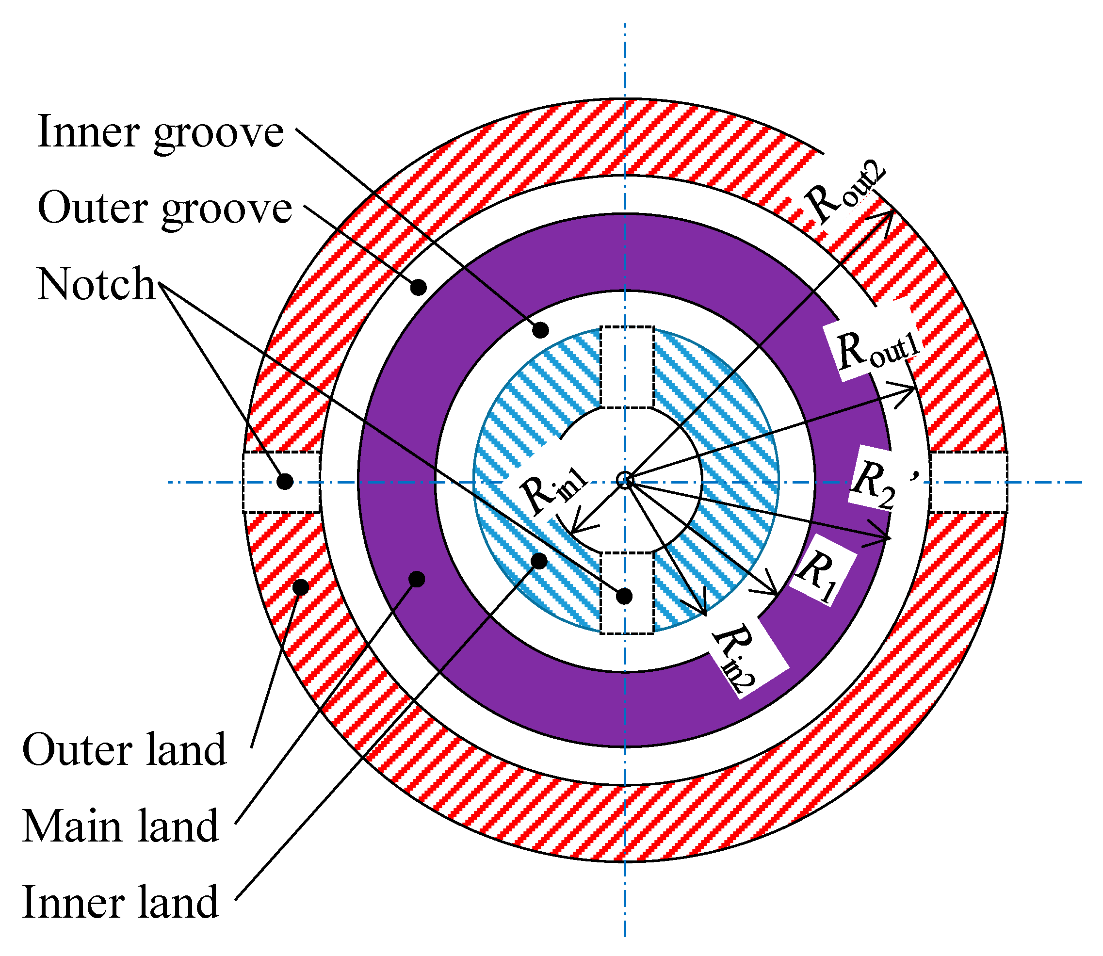
inner radius ratio of main land, = R 1 / R 2
a outer radius ratio of main land, = R 2 / R 2
a i n 1 inner radius ratio of inner land, = R i n 1 / R 2
a i n 2 outer radius ratio of inner land, = R i n 2 / R 2
a o u t 1 inner radius ratio of outer land, = R o u t 1 / R 2
a o u t 2 outer radius ratio of outer land, = R o u t 2 / R 2
d e separation
E ˜ H equivalent elastic modulus, = E / ( p s 0 R 2 2 S 0 )
Hrepresentative clearance
H ˜ a hardness, = H a / ( p s 0 R 2 2 S 0 )
hclearance, = h / H
h ¯ c center thickness
h T mean film thickness
I ¯ moment inertia, = Ω 2 H I / ( p s 0 R 2 4 S 0 )
K bulk modulus
L ¯ power loss, = L / ( Ω p s 0 R 2 3 S 0 )
M ¯ moment, = M / ( p s 0 R 2 3 S 0 )
m ¯ mass, = Ω 2 H m / ( p s 0 R 2 2 S 0 )
p ¯ pressure, = p / ( p s 0 S 0 )
p ¯ e ambient pressure, = p e / ( p s 0 S 0 )
p ¯ r recess pressure, = p r / ( p s 0 S 0 )
p ¯ s supply pressure, = p s / ( p s 0 S 0 )
Qflow rate, = Q / ( Ω R 2 3 )
Q ¯ o u t leaked flow rate, = Q o u t / ( Ω R 2 3 )
R 0 revolution radius
R 2 representative radius
r ¯ ,   θ ,   z ¯ coordinates, = r/R2, θ, z/H
r w load eccentricity
S 0 parameter, = 6 μ Ω ( R 2 / H ) 2 / p s 0
T ¯ friction torque, = T / ( p s 0 R 2 3 S 0 )
V ¯ r recess volume, = 6 μ Ω V r / ( H 2 K R 2 2 )
W ¯ load, = W / ( p s 0 R 2 2 S 0 )
w p plasticity index
X ,   Y ,   Z coordinates
x ,   y ,   z coordinates
α ¯ pad inclination angle, = α R 2 / H
β restrictor parameter, = 4 H 3 l c / ( 3 r c 4 )
β equivalent radius of asperity summit
ζ 0 hydrostatic balance ratio
η asperity density
λ ¯ stiffness, = λ H / ( p s 0 R 2 2 S 0 )
μ viscosity
σ surface roughness, = ( σ 1 2 + σ 2 2 ) 1 / 2
σ standard deviation of asperity summit height
τ time, = Ω t
ϕ pad azimuth
Ω representative angular velocity
Ω disk angular velocity
ω pad angular velocity
Subscripts:
aasperity, contact
ccenter
ffluid
griinner groove
groouter groove
ininner land
mtime-average
maxmaximum
minminimum
mnmain land
outouter land
rrecess
0reference, high pressure period
1inside
2outside

Appendix A

The flow rate in the clearance can be given by
Q ( r ) = 0 2 π q r r   d θ
wherein,
q r = ϕ h 3 12 μ p f r + Ω R 0 sin θ 2 ( h T + σ ϕ s )
Substituting Equation (A2) into Equation (A1) and introducing the dimensionless quantities,
Q ¯ ( r ¯ ) = R 2 r ¯ Ω R 2 3 0 2 π [ ϕ H 3 h ¯ 3 12 μ 6 μ Ω ( R 2 / H ) 2 p ¯ f R 2 r ¯ + Ω R 2 R ¯ 0 sin θ 2 ( H h ¯ T + σ ϕ s ) ]   d θ
Finally, Equation (15) can be obtained.
On the other hand, the torque based on contact friction can be given by
T a 1 = A R d F a 1
wherein,
d F a 1 = ξ τ p [ τ e τ p d A e + d A p ] + ( 1 ξ ) τ a d d A r
where, ξ is area ratio of solid-contact-asperities, τ is shear strength, and the subscript ad is adsorbing film [17]. Additionally, the length R is defined by
R = R 0 2 + r 2 2 R 0 2 r cos ( π θ )
Substituting Equation (A5) into Equation (A4) and introducing the dimensionless quantities, Equation (17) can be obtained.
Further, the torque based on fluid friction can be given by
T f 1 = r 0 2 π R τ 1 r d θ d r
wherein,
τ 1 = μ ( U 2 U 1 ) h ( ϕ f ϕ ^ f s ) ϕ f p h 2 p ¯ f R Θ
and
U 1 = Ω R 0 sin θ sin ( θ Θ ) + Ω ( R 0 cos θ + r ) cos ( θ Θ )   U 2 = ω r cos ( θ Θ ) }
Substituting Equations (A7) and (A8) into Equation (A4), including the definition of ϕ f s [20], and introducing the dimensionless quantities, Equation (18) can be obtained.

Appendix B

The flow chart of the numerical calculation is outlined in Figure A1. First the parameters and the initial values are set; h ¯ c , p ¯ r , Φ ¯ x , and Φ ¯ y are solved by the Runge-Kutta method, while p ¯ a , p ¯ f , Q ¯ , M ¯ a , M ¯ f , W ¯ a , and W ¯ f are computed and L ¯ , T ¯ a , T ¯ f , α ¯ , and ϕ are calculated. When a cycle ends, the initial and final values of h ¯ c , p ¯ r , Φ ¯ x , and Φ ¯ y are compared. If these values are different, the initial values of the next step are set with the final values of the present step and the calculation is continued iteratively. After these values are converged, the time pitch is halved and further the calculation is pursued. Finally, L ¯ m and λ ¯ are calculated and the solutions are output.
Figure A1. The flow chart of calculation.
Lubricants 07 00055 g0a1

References

  1. Shute, N.A.; Turnbull, D.E. Minimum power loss of hydrostatic slipper bearings for axial piston machines. Proc. Int. Conv. Lubr. Wear 1963, 6, 3–14. [Google Scholar]
  2. Böinghoff, O. Untersuchen zum Reibungsverhalten der Gleitschuhe in Schrägscheiben-Axialkolbenmascinen. VDI Forsch. 1977, 584, 1–46. [Google Scholar]
  3. Iboshi, N.; Yamaguchi, A. Characteristics of a slipper bearing for swash plate type axial piston pumps and motors: 1st report, theoretical analysis. Bull. Jpn. Soc. Mech. Eng. 1982, 25, 1921–1930. [Google Scholar] [CrossRef]
  4. Koç, E.; Hooke, C.J. Considerations in the design of partially hydrostatic slipper bearings. Tribol. Int. 1997, 30, 815–823. [Google Scholar] [CrossRef]
  5. Manring, N.D. The relative motion between the ball guide and slipper retainer within an axial-piston swash-plate type hydrostatic pump. J. Dyn. Syst. Meas. Control Trans. ASME 1999, 121, 518–523. [Google Scholar] [CrossRef]
  6. Suzuki, K.; Suzuki, M.; Sakurai, S.; Hemmi, M.; Kazama, T. Multi body dynamics of a slipper in swash plate type piston pumps and motors couples with hydrodynamic analysis of oil-film. Bull. Jpn. Soc. Mech. Eng. 2014, 80, FE0224. (In Japanese) [Google Scholar] [CrossRef]
  7. Schenk, A.; Ivantysynova, M.A. Transient thermoelastohydrodynamic lubrication model for the slipper/swashplate in axial piston machines. J. Tribol. Trans. ASME 2015, 137, 031701–031710. [Google Scholar] [CrossRef]
  8. Lin, S.; Hu, J. Tribo-dynamic model of slipper bearings. Appl. Math. Model. 2015, 39, 548–558. [Google Scholar] [CrossRef]
  9. Hashemi, S.; Kroker, A.; Bobach, L.; Bartel, D. Multibody dynamics of pivot slipper pad thrust bearing in axial piston machines incorporating thermal elastohydrodynamics and mixed lubrication model. Tribol. Int. 2016, 96, 57–76. [Google Scholar] [CrossRef]
  10. Bergada, J.M.; Watton, J.; Haynes, J.M.; Davies, D.L. The hydrostatic/hydrodynamic behaviour of an axial piston pump slipper with multiple lands. Meccanica 2010, 45, 58–602. [Google Scholar] [CrossRef]
  11. Chen, J.; Ma, J.; Li, J.; Fu, Y. Performance optimization of grooved slippers for aero hydraulic pumps. Chin. J. Aeronaut. 2016, 29, 814–823. [Google Scholar] [CrossRef] [Green Version]
  12. Schenk, A.T. Predicting Lubrication Performance between the Slipper and Swashplate in Axial Piston Hydraulic Machines. Ph.D. Thesis, Purdue University, West Lafayette, IN, USA, 2014. [Google Scholar]
  13. Kazama, T. Mathematical modeling of a multi-land slipper for swash-plate type axial piston pumps and motors. In Proceedings of the 5th China-Japan Joint Workshop on Fluid Power, Beijing, China, 23 July 2018; pp. 46–50. [Google Scholar]
  14. Tang, H.; Yin, Y.; Ren, Y.; Xiang, J.; Chen, J. Impact of the thermal effect on the load-carrying capacity of a slipper pair for an aviation axial-piston pump. Chin. J. Aeronaut. 2018, 31, 395–409. [Google Scholar] [CrossRef]
  15. Hashemi, S.; Friedrich, H.; Bobach, L.; Bartel, D. Validation of a thermal elastohydrodynamic multibody dynamics model of the slipper pad by friction force measurement in the axial piston pump. Tribol. Int. 2017, 115, 319–337. [Google Scholar] [CrossRef]
  16. Kazama, T. Thermohydrodynamic lubrication model applicable to a slipper of swashplate type axial piston pumps and motors (Effects of operating conditions). Tribol. Online 2010, 5, 250–254. [Google Scholar] [CrossRef]
  17. Yamaguchi, A.; Matsuoka, H. A mixed lubrication model applicable to bearing/seal parts of hydraulic equipment. J. Tribol. Trans. ASME 1992, 114, 116–121. [Google Scholar] [CrossRef]
  18. Kazama, T.; Yamaguchi, A. Application of a mixed lubrication model for hydrostatic thrust bearings of hydraulic equipment. J. Tribol. Trans. ASME 1993, 115, 686–691. [Google Scholar] [CrossRef]
  19. Greenwood, J.A.; Williamson, J.B.P. Contact of nominally flat surfaces. Proc. R. Soc. Lond. 1996, 295, 300–319. [Google Scholar] [CrossRef]
  20. Patir, N.; Cheng, H.S. An average flow model for determining effects of three-dimensional roughness on partial hydrodynamic lubrication. J. Lubr. Technol. Trans. ASME 1978, 100, 12–17. [Google Scholar] [CrossRef]
  21. Patir, N.; Cheng, H.S. Application of average flow model to lubrication between rough sliding surfaces. J. Lubr. Technol. Trans. ASME 1979, 101, 220–230. [Google Scholar] [CrossRef]
  22. Kazama, T.; Yamaguchi, A. Experiment on mixed lubrication of hydrostatic thrust bearings for hydraulic equipment. J. Lubr. Technol. Trans. ASME 1995, 117, 399–402. [Google Scholar] [CrossRef]
  23. Kazama, T. Numerical simulation of a slipper model for water hydraulic pumps/motors in mixed lubrication. In Proceedings of the 6th JFPS International Symposium on Fluid Power, Tsukuba, Japan, 7–10 November 2005. [Google Scholar] [CrossRef]
  24. Kazama, T. Numerical simulation of a slipper with retainer for axial piston pumps and motors under swashplate vibration. JFPS Int. J. Fluid Power Syst. 2017, 10, 18–23. [Google Scholar] [CrossRef]
Figure 1. The coordinates of the slipper model.
Lubricants 07 00055 g001
Figure 2. Schematic of the sliding surface of the multi-land slipper.
Lubricants 07 00055 g002
Figure 3. Changes in supply pressure p s / p s 0 and load W / W 0 .
Lubricants 07 00055 g003
Figure 4. The comparison of changes in the center clearance h ¯ c and minimum clearance h ¯ min .
Lubricants 07 00055 g004
Figure 5. The comparison of changes in the pad inclined angle α ¯ and the pad azimuth ϕ.
Lubricants 07 00055 g005
Figure 6. The comparison of changes in the maximum contact pressure p ¯ a , max and leakage flow rate Q ¯ o u t .
Lubricants 07 00055 g006
Figure 7. The comparison of changes in the cavitating area ratio A ¯ c a v / A ¯ 0 and the contacting area ratio A ¯ c n t / A ¯ 0 .
Lubricants 07 00055 g007
Figure 8. The effects of supply pressure p s on the pad swing angle Δ ϕ .
Lubricants 07 00055 g008
Figure 9. The effects of supply pressure p s on normalized maximum contact pressure p ¯ a , max and the leakage flow rate Q ¯ o u t .
Lubricants 07 00055 g009
Figure 10. The effects of supply pressure p s on normalized mean power loss L ¯ m and stiffness λ ¯ .
Lubricants 07 00055 g010
Figure 11. The effects of supply pressure p s on the ratio of leakage power loss to total power loss L ¯ m Q / L ¯ m .
Lubricants 07 00055 g011
Figure 12. The effects of rotational speed N on the pad swing angle Δ ϕ .
Lubricants 07 00055 g012
Figure 13. The effects of rotational speed N on normalized maximum contact pressure p ¯ a , max and the leakage flow rate Q ¯ o u t .
Lubricants 07 00055 g013
Figure 14. The effects of rotational speed N on normalized mean power loss L ¯ m and stiffness λ ¯ .
Lubricants 07 00055 g014
Figure 15. The effects of rotational speed N on ratio of leakage power loss to total power loss L ¯ m Q / L ¯ m .
Lubricants 07 00055 g015
Table 1. Representative numerical parameters.
ParameterValueUnit
a i n 1 0.5
a i n 2 0.6
a 0.7
a 0.8
a o u t 1 0.9
a o u t 2 1
K 1GPa
m 100g
R 0 / R 2 2.4
R 2 12.5mm
r c 0.3mm
r w / R 2 0.08
ζ 0 1.1
μ 28mPa·s
ρ 875kg/m3
σ 1μm

