Probability of Face Contact for a High-Speed Pressurised Liquid Film Bearing Including a Slip Boundary Condition

Abstract

An initial deterministic mathematical model for the dynamic motion of a simple pressurised liquid film bearing is derived and utilised to evaluate the possibility of bearing contact for thin film operation. For a very thin film bearing the flow incorporates a Navier slip boundary condition as parametrised by a slip length that in general is subject to significant variability and is difficult to determine with precision. This work considers the formulation of a modified Reynolds equation for the pressurised liquid flow in a highly rotating coned bearing. Coupling of the axial motion of the stator is induced by prescribed axial oscillations of the rotor through the liquid film. The bearing gap is obtained from solving a nonlinear second-order non-autonomous ordinary differential equation, via a mapping solver. Variability in the value of the slip length parameter is addressed by considering it as a random variable with prescribed mean and standard deviation. The method of derived distributions is used to exactly quantify the impact of variability in the slip length with a parametric study investigating the effect of both the deterministic and distribution parameters on the probability of contact. Additionally, as the axial rotor oscillations also have a random aspect due to possible varying excitations of the system, the probability of contact is investigated for both random amplitude of the periodic rotor oscillations and random slip length, resulting in a two parameter random input problem. The probability of contact is examined to obtain exact solutions and evaluate a range of bearing configurations.

1. Introduction

Pressurised liquid film bearings are considered in this work consisting of two structural components, a rotor and stator, separated by a thin liquid film which experiences relative rotational motion. The thin liquid film is used to maintain a separation between the rotating and stationary elements under external axial loads on the bearing through the generation of a local film pressure. In practice, these bearings operate as a combined hydrostatic and hydrodynamic bearing where the fluid gap is maintained by the pressurised fluid and the dynamics of the bearings rotational motion. In some practical applications such bearings operate at very high rotational speeds, requiring the inclusion of additional centrifugal inertia effects which are not considered in the classical lubrication formulation of this type of problems (Reynolds equation). Under these conditions, the bearing design requires precise detailed knowledge of variation in the bearing gap during operating condition in order to evaluate possible contact between the rotor and stator.

Analysis of a pressurised fluid film bearing with parallel surfaces is given for a Newtonian flow with a no-slip condition by Garratt et al. [1] where the bearing structure was coupled to the pressurised fluid flow and the dynamics investigated when the lower face undergoes prescribed periodic axial oscillations. A more general geometry with the inclusion of a coned rotor (tapered surfaces) was considered by Bailey et al. [2], allowing more extensive bearing gap investigations. The bearing axial dynamics were examined for prescribed periodic axial oscillations including those of amplitude larger than the equilibrium film thickness. Results indicated that the film thickness can become very small, even reaching film gaps at nano and micro scales. At these scales, surface effects start to dominates over volume related phenomena, requiring accurate details of the flow surface interaction. In a continuous approximation of fluid motions at very small scales, nano and micro, surface slip velocity conditions are typically considered to take into account the additional surface effects. Incorporation of a slip condition on the bearing faces in the analysis of highly rotating parallel bearings with a small face clearance by Bailey et al. [3] showed the bearing faces do not have contact, although the fluid film can become very small. However, for the case of a coned bearing geometry with a slip boundary condition, Bailey et al. [4] showed face contact is possible.

Thin film gas flow regimes over an atomically smooth surface are classified by the Knudsen number, $K_n=l/{\widehat{h}}_0$, where l is the fluid mean free path corresponding to the collision distance between molecules (for air at atmospheric conditions $l=68$ nm) and ${\widehat{h}}_0$ is the characteristic fluid thickness. For flow with a Knudsen number between ${10}^{-3}$ and ${10}^{-1}$, denoting micro and nano scales, a continuum flow model with a slip boundary condition is usually employed. Navier [9] was the first to predict the existence of velocity slip, proposing a slip model based on a linear relationship between the tangential shear rate and the fluid-solid tangential velocity difference, and with the slip length as the proportionality constant.

The slip condition for liquid flows are however not as well defined as in gas flows. For liquid flowing over a hydrophobic solid surface, an apparent slip velocity has been observed just above the solid surface, with a slip length of the order of 1 μm and even of the order of 50 μm in the case of super hydrophobic surfaces [11,12]. For a hydrophilic surface, a no-slip boundary condition is usually employed in the analysis of liquid flows at micro and nano scale. However experimental studies examining specific chemical and electrochemical conditions of both the solid and liquid showed slip velocities can exist, which are attributed to the effect of the extra reactions on the wettability of the liquid and the potential absorption into the solid surface [13,14]. Typical experimental and theoretical studies on the existence of slip velocity at micro and nano scales, are given by [5,6,7,8].

The numerical simulation of a thin film, with thickness of the order of magnitude of the irregular surface roughness, becomes extremely difficult due to the requirement of imposing the no-slip velocity condition on the corresponding irregular boundary. In these cases, it is possible to replace the no-slip boundary condition over the irregular surface by an effective slip boundary condition onto an equivalent smooth surface, with the slip length of the order of the size of the surface roughness (see [15] and [16]). An example is the average surface roughness, $R_a$, of stainless steel that can range from $0.1\mu m\le R_a\le 1\mu m$, according with surface finishes technology employed. An approach employed by several authors is to find an asymptotically equivalent slip length for small-scale variations of the surface roughness boundary using homogenization theory, (see [17]).

More generally the mathematical formulation and associated numerical simulation of fluid film flow motions, at the nano and micro scale, makes use of slip velocity conditions, where the slip length can range from the size of the surface roughness to the fluid thickness or higher.

This work considers the dynamic analysis of liquid film bearing under extreme conditions, where the fluid gap can attain a thickness of nano or micro scale size. Included are hydrophobic surface bearings, with slip length of the order of the liquid film thickness or larger, as well as hydrophilic surfaces, where the slip length is of the order of the bearings surface roughness.

Precise evaluation of the slip length is restricted due to limitations of the simulations [18] and incorrect interpretation of results [19]. Experimental investigation of the slip length requires length scales comparable to the slip length to be examined, therefore extremely accurate techniques with high spatial resolution, capable of interfacial flow measurements are needed [20]. Indirect experimental methods measure macroscopic flow quantities [21] but can suffer from limited spacial resolution, with the slip velocity inferred from using techniques which can rely on tentative theoretical models [22]. Direct methods also suffer from limited spatial resolution [23], with the fluid flow velocity, which may measure only a few nanometres, are typically determined in an interrogation area which is several hundred nanometres in size [24] leading to potential errors in measurements.

Increased interest exists on accounting for greater predictability of the dynamic behaviour in industrial bearing designs. These are typically complex, with associated mathematical models involving large numbers of parameters that may only be known approximately. Sources of uncertainty in a bearing model include the slip flow at the fluid-solid interface and from the random axial motion of the rotor due to external excitations.

Uncertainty in a bearing model and dynamical system originating from external excitations has been examined using a variety of methods, typically based on Monte Carlo techniques [25]. In this case, sampling is directly from the random input parameter with the output of the deterministic model evaluated at each input sample. This is a robust process able to deal with complex situations and a large number of uncertain input parameters, however an extensive number of code executions may be required to produce sufficiency accurate results. To minimise cost and efficiency additional theoretical methods for uncertainty quantification have been developed, such as polynomial chaos, Gaussian process emulator and Markov Chain Monte Carlo method.

In Zigang et al. [26], the dynamic response and vibration characteristics of two in-line rotor bearing systems are examined to quantify the effects of uncertainty. The equations of motion of the rotor system are derived and stochastic modelling for uncertainty in the damping and nonlinear support stiffness is developed, based on the polynomial chaos expansion technique in a stochastic framework. Monte-Carlo simulation is used as a comparison, with good agreement reported between the two methods. Response statistics and the dynamic behaviour of the stochastic system are examined through the mean and probability density function. Results show the uncertainties in the nonlinear support stiffness and damping have a significant effect on the predicted behaviour of the rotor system, and increasing the random intensities causes the realisation amplitudes to span a wider band of amplitudes.

In the special case where a comprehensive deterministic mathematical model is available, a subjective interpretation of probability, the method of derived distributions [27], can be used to exactly quantify the effects of random input parameters. Describing the random input parameters by a probability distribution function and using the deterministic relationship between the input and output parameters enables the probability density function and cumulative density function of the output to be determined exactly. Statistical analysis can be conducted on the resulting realisations allowing the relevant statistical properties of the process to be extracted.

A main focus of this work is to analyse the probability of contact in an important application requiring a mathematical and numerical model for a high speed pressurised liquid film coned bearing with a slip boundary condition and prescribed periodic axial oscillations of the rotor; the deterministic model is based on the work by Bailey et al. [4]. The governing Reynolds equation for slip flow is derived by incorporating a constant slip model with a linear relationship between the tangential shear rate and the fluid-wall velocity differences with a slip length as the proportionality constant. The probability of bearing face contact is examined using the method of derived distributions to investigate the lack of precise knowledge of the slip length. To account for variability in the slip length and amplitude of rotor oscillations, these parameters are considered as random variables with prescribed mean and standard deviation to investigate the probability of face contact through a parametric study.

Although in liquid film bearings design, the use of a tapered surface is considered to increase the liquid loading force in order to maintain a desirable film thickness at operating conditions, in this work it has been found that this can lead to undesirable aspects under extreme conditions. If during the dynamic response of the bearing, under an external force, the liquid gap reaches a thickness of nano or micro scale, the tapered surface can induce possible stator-rotor collision (contact) dependant on the liquid slip velocity condition.

An approach is provided for determining the probability of contact at different operating conditions to inform bearing design criteria. It is noted that for controlling the possible displacements of the rotor due to external forces, using structural constraints, the dynamic response of the bearing may encounter very small fluid gaps and the use of a tapered surface needs to be carefully evaluated. This may be only used where necessary and the corresponding angle needs to be limited to a small value.

2. Deterministic Mathematical Model

A simplified mathematical model of a high speed pressurised fluid film bearing for a coned rotor and incorporating a slip boundary condition is developed, following Bailey et al. [4]. A model for the incompressible fluid flow through the bearing is derived from the Navier-Stokes momentum and continuity equations in axisymmetrical coordinates. To express the mathematical formulation of the problem in dimensionless variables, a characteristic bearing radius ${\widehat{r}}_0$, film thickness ${\widehat{h}}_0$, rotor velocity $\widehat{\Omega }\widehat{r}$ and differential pressure $\Delta \widehat{P}$, due to imposed pressure at inner radius ${\widehat{r}}_I$ and outer radius ${\widehat{r}}_O$ are defined with dimensionless time variable $t=\widehat{\omega }\widehat{t}$ where $\widehat{\omega }$ is the angular frequency. Dimensionless velocities are taken to be $\widehat{u}/{\widehat{h}}_0^2\Delta \widehat{P}{\left(\mu ({\widehat{r}}_O-{\widehat{r}}_I)\right)}^{-1}$, $\widehat{v}/\widehat{\Omega }{\widehat{r}}_0$ and $\widehat{w}/{\widehat{h}}_0{\widehat{T}}^{-1}$ with dimensionless radius and height given by $r=\widehat{r}/{\widehat{r}}_0$ and $z=\widehat{z}/{\widehat{h}}_0$ respectively. The dimensionless slip length is given by $l_s=\widehat{l_s}/{\widehat{h}}_0$ and for a thin film bearing the aspect ratio ${\delta }_0={\widehat{h}}_0/{\widehat{r}}_0$ is small ${\delta }_0\ll 1$.

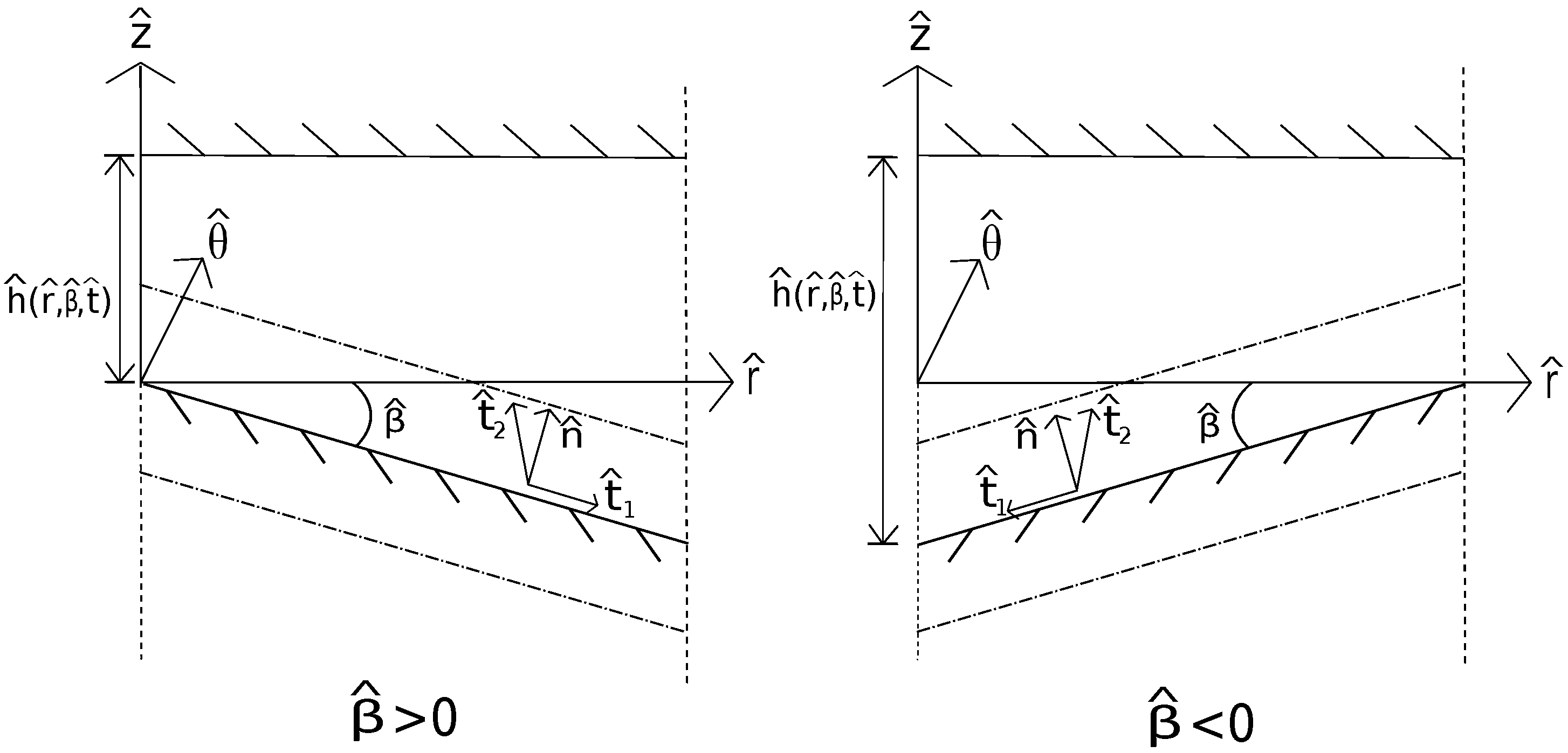
The rotor has a fixed coning angle, assumed to be small giving $cos\widehat{\beta }\simeq 1$ and $sin\widehat{\beta }\simeq \widehat{\beta }$, leading to the scaling $\widehat{\beta }=\beta {\delta }_0$ with $\beta =O\left(1\right)$, giving consistency with the lubrication condition, such that $\partial h_r/\partial r\simeq -\beta$. Cases of a positively and negatively coned bearing are considered separately as is shown in Figure 1, referred to as a PCB and NCB, respectively. For a bearing containing a coned rotor undergoing prescribed periodic oscillations, the dimensionless film thickness is given by

$$\begin{array}{c}h(r,\beta ,t)=h_s\left(t\right)-\epsilon sint+(r-a)\beta \text{for}\beta >0\hfill \end{array}$$

$$\begin{array}{c}h(r,\beta ,t)=h_s\left(t\right)-\epsilon sint+(r-1)\beta \text{for}\beta <0\hfill \end{array}$$

(1)

where $h_s\left(t\right)$ is the height of the axially displaced stator, $\epsilon sint$ the axial forcing of the rotor with amplitude ε and $a={\widehat{r}}_I/{\widehat{r}}_0$ is a measure of the bearing width, $0<a<1$.

Figure 1. Axially symmetric geometry and notation of a positively coned bearing (PCB) $\beta >0$ and negatively coned bearing (NCB) $\beta <0$.

Figure 1. Axially symmetric geometry and notation of a positively coned bearing (PCB) $\beta >0$ and negatively coned bearing (NCB) $\beta <0$.

The associated radial Reynolds number is given by $R{e}_U=\widehat{\rho }{\widehat{h}}_0\widehat{U}/\widehat{\mu }$, where $\widehat{\rho }$ is the density and $\widehat{\mu }$ the dynamic viscosity. To ensure that the effects of viscosity are retained at leading order the pressure is scaled as $\widehat{P}=\widehat{\mu }{\widehat{r}}_0\widehat{U}/{\widehat{h}}_0^2$. Classical lubrication theory neglects inertia due to the reduced Reynolds number $R{e}_U{\delta }_0\ll 1$, however, as in Garratt et al. [1], the centrifugal inertia is retained to include cases of high rotational speed bearing operations for which terms of the order $R{e}_U{\delta }_0{\left(R{e}^{*}\right)}^2$ are considered to be of $O\left(1\right)$, with ${\left(R{e}^{*}\right)}^2={(\widehat{\Omega }{\widehat{r}}_0/\widehat{U})}^2\gg 1$. The squeeze number $\tilde{\sigma }={\widehat{r}}_0/\left(\widehat{U}\widehat{T}\right)$ characterises any time dependent effects whilst the Froude number $Fr=\widehat{U}/{\left(\widehat{g}{\widehat{h}}_0\right)}^{1/2}$, where $\widehat{g}$ is the acceleration due to gravity, parametrises the importance of the gravitational effects relative to the radial flow. However, gravity can be neglected given $R{e}_U{\delta }_{0}F{r}^{-2}\ll 1$; this is consistent with lubrication theory provided the Froude number is $O\left(1\right)$.

In the case of slip flow, as considered by Bailey et al. [4], the velocity boundary condition on a bearing face comprise of a jump in the tangential velocities across the fluid-solid interface corresponding to the slip velocity induced due to wall shear, i.e., a Navier slip condition. Continuity of the normal velocity across the fluid-solid interface is imposed along with a no flux condition. Thus the velocity boundary conditions on the rotor and stator, denoted by superscript r and s, respectively, are given by

$$\begin{array}{c}\hfill \widehat{\mathbf{u}}·{\widehat{\mathbf{t}}}_1-{\widehat{\mathbf{u}}}^r·{\widehat{\mathbf{t}}}_1=2\widehat{l_s}{\widehat{e}}_{ij}{\widehat{n}}_j^r{\widehat{t}}_{1,i},\widehat{\mathbf{u}}·{\widehat{\mathbf{t}}}_2-{\widehat{\mathbf{u}}}^r·{\widehat{\mathbf{t}}}_2=2\widehat{l_s}{\widehat{e}}_{ij}{\widehat{n}}_j^r{\widehat{t}}_{2,i},\widehat{\mathbf{u}}·{\widehat{\mathbf{n}}}^r-{\widehat{\mathbf{u}}}^r·{\widehat{\mathbf{n}}}^r=0,\text{at}\widehat{z}=\widehat{h_r}\end{array}$$

$$\begin{array}{c}\hfill \widehat{\mathbf{u}}·{\widehat{\mathbf{t}}}_3-{\widehat{\mathbf{u}}}^r·{\widehat{\mathbf{t}}}_3=2\widehat{l_s}{\widehat{e}}_{ij}{\widehat{n}}_j^s{\widehat{t}}_{3,i},\widehat{\mathbf{u}}·{\widehat{\mathbf{t}}}_4-{\widehat{\mathbf{u}}}^r·{\widehat{\mathbf{t}}}_4=2\widehat{l_s}{\widehat{e}}_{ij}{\widehat{n}}_j^s{\widehat{t}}_{4,i},\widehat{\mathbf{u}}·{\widehat{\mathbf{n}}}^s-{\widehat{\mathbf{u}}}^r·{\widehat{\mathbf{n}}}^s=0,\text{at}\widehat{z}=\widehat{h_s}\end{array}$$

(2)

where the right hand side of the above equations are due to the surface shear stress with proportionality constant $\widehat{l_s}$ and rate of strain tensor ${\widehat{e}}_{ij}$. The rotor velocity components are given by ${\widehat{\mathbf{u}}}^r=(\partial \widehat{h_r}/\partial \widehat{t},0,\widehat{\Omega }\widehat{r})$ corresponding to prescribed axial motion and fixed azimuthal rotation and the stator is allowed to move axially due to the interaction with the fluid, giving the stator velocity as ${\widehat{\mathbf{u}}}^s=(\partial \widehat{h_s}/\partial \widehat{t},0,0)$.

Due to the additional slip component on the bearing face both the normal and tangential velocities on the rotor and stator are required. A PCB and NCB are considered separately, denoted by subscripts + and −, respectively, in the coordinate system $(\widehat{z},\widehat{r},\widehat{\theta })$ with velocities $\widehat{\mathbf{u}}=(\widehat{w},\widehat{u},\widehat{v})$. Figure 1 shows the normal rotor vector ${\widehat{\mathbf{n}}}^r$ and two orthogonal tangential vectors ${\widehat{\mathbf{t}}}_1$ and ${\widehat{\mathbf{t}}}_2$ on the rotor face in the cases of a PCB and NCB. The normal and azimuthal tangent are given by

$$\begin{array}{c}\hfill {\widehat{\mathbf{n}}}^r=(cos\widehat{\beta },sin\widehat{\beta },0),{\widehat{\mathbf{t}}}_2=(0,0,1)\end{array}$$

(3)

respectively, and the axial tangents are

$$\begin{array}{c}{\widehat{\mathbf{t}}}_{1,+}=(-sin\widehat{\beta },cos\widehat{\beta },0),{\widehat{\mathbf{t}}}_{1,-}=(sin\widehat{\beta },-cos\widehat{\beta },0)\hfill \end{array}$$

(4)

Cases of a PCB and NCB, respectively, requiring separate radial velocity boundary conditions to be derived.

The stator lies parallel to the radial direction, giving the normal vector ${\widehat{\mathbf{n}}}^s$ in the negative $\widehat{z}$ direction and two orthogonal tangential components, ${\widehat{\mathbf{t}}}_3$ and ${\widehat{\mathbf{t}}}_4$ on the face of the stator in the radial and azimuthal direction, respectively.

Velocity boundary conditions on the rotor in (2) are given by

$$\begin{array}{ccc}\hfill \widehat{u}cos\widehat{\beta }-\widehat{w}sin\widehat{\beta }& =& -\frac{\partial \widehat{h_r}}{\partial \widehat{t}}sin\widehat{\beta }+\widehat{l_s}\left(\left(\frac{\partial \widehat{u}}{\partial \widehat{z}}+\frac{\partial \widehat{w}}{\partial \widehat{r}}\right)\left({cos}^2\widehat{\beta }-{sin}^2\widehat{\beta }\right)+2\left(\frac{\partial \widehat{u}}{\partial \widehat{r}}-\frac{\partial \widehat{w}}{\partial \widehat{z}}\right)cos\widehat{\beta }sin\widehat{\beta }\right)\hfill \\ \hfill \widehat{v}-\widehat{\Omega }\widehat{r}& =& \widehat{l_s}\left(\widehat{r}\frac{\partial }{\partial \widehat{r}}\left(\frac{\widehat{v}}{\widehat{r}}\right)sin\widehat{\beta }+\frac{\partial \widehat{v}}{\partial \widehat{z}}cos\widehat{\beta }\right)\hfill \\ \hfill \widehat{w}cos\widehat{\beta }+\widehat{u}sin\widehat{\beta }& =& \frac{\partial \widehat{h_r}}{\partial \widehat{t}}cos\widehat{\beta }\hfill \end{array}$$

(5)

using the normal and tangent vectors given in (3) and (4) and the rate of strain tensor components as given in Batchelor [28] (p. 602). In an axisymmetric configuration the azimuthal derivatives do not appear.

The velocity boundary conditions on the stator (2), give

$$\begin{array}{c}\hfill \widehat{u}=-{\widehat{l}}_s\left(\frac{\partial \widehat{u}}{\partial \widehat{z}}+\frac{\partial \widehat{w}}{\partial \widehat{r}}\right),\widehat{v}=-2{\widehat{l}}_s\frac{\partial \widehat{v}}{\partial \widehat{z}},\widehat{w}=\frac{\partial \widehat{h_s}}{\partial \widehat{t}}\end{array}$$

(6)

Under these conditions, the leading order non-dimensional rotor and stator velocity boundary conditions given in (5) and (6), respectively, become

$$\begin{array}{c}\hfill u=l_s\frac{\partial u}{\partial z},v=r+l_s\frac{\partial v}{\partial z},w=\frac{\partial h_r}{\partial t}-\frac{u}{\tilde{\sigma }}\beta ,\text{at}z=h_r\end{array}$$

$$\begin{array}{c}\hfill u=-l_s\frac{\partial u}{\partial z},v=-l_s\frac{\partial v}{\partial z},w=\frac{\partial h_s}{\partial t},\text{at}z=h_s\end{array}$$

(7)

as ${\delta }_0\ll 1$. The only dependence on the coning angle is given in the axial rotor velocity boundary condition.

A governing equation for a bearing with narrow gap, satisfying the slip boundary conditions, is readily obtained from the leading order thin film approximation of the continuity equation, where formally terms of $O\left({\delta }_0\right)$ are neglected, giving the modified Reynolds equation as

$$\begin{array}{l}\sigma \frac{\partial h}{\partial t}-\frac{1}{r}\frac{\partial }{\partial r}\left(r\frac{\partial p}{\partial r}(h^3+6l_s{h}^2)\right)\\ +\frac{\lambda }{r}\frac{\partial }{\partial r}\left(\frac{r^2}{{(h+2l_s)}^2}\left(h^5+10h^4{l}_s+\frac{70}{3}{h}^3{l}_s^2+20h^2{l}_s^3\right)\right)=0\hfill \end{array}$$

(8)

The speed parameter $\lambda =3R{e}_U{\delta }_0{\left(R{e}^{*}\right)}^2/10$ characterises the importance of centrifugal inertia and squeeze number $\sigma =12\tilde{\sigma }$ is rescaled. The Reynolds Equation (8) has no explicit dependence on the coning angle and expresses the relationship between the pressure p and film thickness h. Similar Reynolds equations have been derived for slip flow in a bearing [29,30,31], but neglecting the effects of centrifugal inertia and in [3,4] including inertia effects. Pressure boundary conditions at the inner and outer radii of the bearing are defined in Appendix A, Equation (37).

Axial displacement of the stator is modelled using a spring-mass-damper model, where the stator equilibrium position at steady flow conditions is given by

$$\begin{array}{ccc}\hfill {\widehat{h}}_0& =& {\widehat{h}}_{0s}-\frac{\widehat{m}\widehat{g}}{\widehat{K_z}}\text{for}\beta \ge 0\hfill \end{array}$$

$$\begin{array}{ccc}\hfill {\widehat{h}}_0& =& {\widehat{h}}_{0s}-({\widehat{r}}_O-{\widehat{r}}_I)\widehat{\beta }-\frac{\widehat{m}\widehat{g}}{\widehat{K_z}}\text{for}\beta <0\hfill \end{array}$$

(9)

with $\widehat{m}\widehat{g}$ as the stator weight and ${\widehat{K}}_z$ as the restoring force coefficient (stiffness), respectively. The corresponding dynamic equation of the stator axial position in dimensionless variables is given by

$$\begin{array}{ccc}\hfill \frac{d^2{h}_s}{d{t}^2}+D_a\frac{d{h}_s}{dt}+K_z(h_s-1)& =& \alpha F\left(t\right)\text{for}\beta >0\hfill \end{array}$$

$$\begin{array}{ccc}\hfill \frac{d^2{h}_s}{d{t}^2}+D_a\frac{d{h}_s}{dt}+K_z(h_s-(1-a)\beta -1)& =& \alpha F\left(t\right)\text{for}\beta <0\hfill \end{array}$$

(10)

where $D_a={\widehat{D}}_a/\widehat{m}\widehat{\omega }$ and $K_z={\widehat{K}}_z/\widehat{m}{\widehat{\omega }}^2$ are dimensionless linear damping and restoring force coefficients, respectively. In (10) ${\widehat{D}}_a$ is the damping coefficient and $F\left(t\right)$ is the resultant dimensionless axial force on the stator, defined in Appendix A by Equation (45). The force coupling dimensionless parameter is given by $\alpha =\widehat{\mu }\widehat{U}/\widehat{m}{\widehat{\omega }}^2{\delta }_0^3$ and considered to be of $O\left(1\right)$.

The dynamic Equation (10) for the axial position of the stator, provides the corresponding dimensionless stator equilibrium bearing height, corresponding to the geometric configuration in Figure 1 with film thickness $h=1$ at the inner radius for PCB and at the outer radius for NCB; giving $h_s=1$ for PCB and $h_s=1+(1-a)\beta$ for a NCB, according to Equation (9).

To solve the Reynolds Equation (8) and stator Equation (10) simultaneously, it is mathematically convenient to introduce the time dependent minimum face clearance (MFC) as

$$\begin{array}{cc}\hfill g\left(t\right)=h_s\left(t\right)-h_r(a,t)=h(a,t)-(r-a)\beta ,& \text{if}\beta >0\end{array}$$

$$\begin{array}{cc}\hfill g\left(t\right)=h_s\left(t\right)-h_r(1,t)=h(1,t)-(r-1)\beta ,& \text{if}\beta <0\end{array}$$

(11)

Integration of the Reynolds equation gives explicit analytic expressions for the pressure field and force on the stator, given in Appendix A, Equations (38) and (46), respectively. Substituting the force expression (46) and MFC (11) into the stator Equation (10) yields a nonlinear second-order non-autonomous ordinary differential equation for the MFC given by

$$\begin{array}{c}\hfill \frac{{\mathrm{d}}^{2}g}{\mathrm{d}{t}^2}+D(g,l_s,\beta )\frac{\mathrm{d}g}{\mathrm{d}t}+S(g,\lambda ,l_s,\beta )=\epsilon ((1-K_z)sint-D_{a}cost)\end{array}$$

(12)

where

$$\begin{array}{ccc}& & D(g,l_s,\beta )=D_a-\alpha \pi B(g,l_s,\beta ),S(g,\lambda ,l_s,\beta )=K_z(g-1)-\alpha \pi A(g,\lambda ,l_s,\beta )\hfill \end{array}$$

(13)

for a PCB. Expression for A and B are given in Appendix A, Equations (47) and (48) respectively. A NCB only differs in the term; $S(g,\lambda ,\beta ,l_s)=K_z(g-(1-a)\beta -1)-\alpha \pi A(g,\lambda ,\beta ,l_s)$. Dynamically Equation (12) corresponds to a harmonically forced oscillator with nonlinear damping coefficient $D(g,l_s,\beta )$ and effective restoring force $S(g,\lambda ,l_s,\beta )$.

The total stiffness of the system $K_{zT}$ is found by differentiating the effective restoring force with respect to the MFC, giving

$$\begin{array}{c}\hfill K_{zT}=\frac{\partial S}{\partial g}=K_z-\alpha \pi \frac{\partial A}{\partial g}\end{array}$$

(14)

where $K_z$ is the contribution from the structure and the fluid contribution is given by

$$\begin{array}{ccc}\hfill K_{zf}& =& -\alpha \pi \frac{\partial A}{\partial g}\hfill \\ & =& -\alpha \pi (2(p_O-p_I)-\lambda (1-a^2))\left(\frac{\partial G_I\left(g\right)}{\partial g}\frac{1}{G(g,1)}-\frac{G_I\left(g\right)}{G{(g,1)}^2}\frac{\partial G(g,1)}{\partial g}\right)\hfill \end{array}$$

(15)

using the definition for A in (47). The functions G and $G_I/g$ are given in Appendix A, Equations (42) and (50), respectively, with derivatives $\partial G/\partial g$ and $\partial G_I/\partial g$ taken as the derivative with respect to the MFC.

In the case of a non-pressurised parallel bearing the fluid stiffness is given by

$$\begin{array}{c}\hfill K_{zf}=\lambda \alpha \pi \frac{{l_s}^{2}g(7g+30l_s)}{3{(g+6l_s)}^2{(g+2l_s)}^3}\left(1-a^4+\frac{{(1-a^2)}^2}{lna}\right)\end{array}$$

(16)

It is noted that in the case of a non-pressurised parallel bearing using classical lubrication theory, i.e., neglecting inertial effect and slip condition, predictions give zero contribution of the stiffness of the system from the fluid component.

2.1. Numerical Scheme

It is anticipated that for a fixed value of the slip length, $l_s$, and rotor oscillation of period T, the nonlinear non-autonomous dynamic system (12) admits periodic solutions. Numerical schemes that are able to predict periodic solutions of nonlinear differential equations are not always reliable and require special considerations. In this work a numerical technique is implemented using a stroboscopic map to obtain the solution in a prescribed period T.

Periodic solutions to Equation (12) are denoted by the vector $\mathbf{g}(g\left(t\right),\tilde{f}\left(t\right))$ with $\tilde{f}=dg/dt$ and corresponding values of $(g\left(t\right),\tilde{f}\left(t\right))$ at the beginning of the period given by $g\left(t_0\right)=g_0$, and $\tilde{f}\left(t_0\right)={\tilde{f}}_0$, which are denoted here as the initial conditions of the periodic motion and considered as unknown in the numerical algorithm for increasing slip lengths. Periodicity is obtained when the values of the solution at the end of the period are identical to their initial conditions, i.e., $g\left(T\right)=g_0$, and $\tilde{f}\left(T\right)={\tilde{f}}_0$.

In the numerical algorithm, the second order differential Equation (12) is expressed as the following system of first order coupled differential equations:

$$\begin{array}{c}\hfill \frac{dg}{dt}=\tilde{f}\text{and}\frac{\mathrm{d}\tilde{f}}{\mathrm{d}t}=-D\left(g\left(t\right)\right)\tilde{f}-S\left(g\left(t\right)\right)+Ysin(t+\varphi )\end{array}$$

(17)

The numerical scheme consists of developing a mapping function that advances any initial condition ${\mathbf{g}}_0$ at time $t_0$ by a time T, defining a stroboscopic map ${\varphi }^{\prime }(T;{\mathbf{g}}_0,t_0)$. This ${\Re }^2\to {\Re }^2$ map integrates the system of Equations (17) forward through one period of the rotor oscillations. To identify periodic solutions, the fixed points of the stroboscopic map $\mathbf{g}\left(t\right)=\mathbf{g}(t+T)$ are found iteratively which corresponds to the condition

$$\begin{array}{c}\hfill \mathbf{g}\left(T\right)-\mathbf{g}\left(t_0\right)={\mathit{\varphi }}^{\prime }(T;{\mathbf{g}}_0,t_0)-{\mathbf{g}}_0=\mathbf{G}({\mathit{\varphi }}^{\prime }(T;{\mathbf{g}}_0,t_0),{\mathbf{g}}_0)=0\end{array}$$

(18)

giving periodic solutions $\mathbf{g}(g\left(t\right),\tilde{f}\left(t\right))$.

Solutions are found numerically from an iterative Newton’s method, given an initial guess value ${\tilde{\mathbf{g}}}_0$. Successively improved iterates ${\mathbf{g}}_0$ are given from the numerical iterative scheme

$$\begin{array}{c}\hfill {{\mathbf{g}}_0}_{n+1}={\widetilde{{\mathbf{g}}_0}}_n-\mathbf{J}{\left(T\right)}^{-1}(\mathbf{g}\left(T\right)-{\widetilde{{\mathbf{g}}_0}}_n)\end{array}$$

(19)

where the Jacobian matrix is given by

$$\begin{array}{c}\hfill \mathbf{J}\left(T\right)=\frac{\partial \mathbf{G}({\mathit{\varphi }}^{\prime },{\mathbf{g}}_0)}{\partial {\mathbf{g}}_0}=\left[\begin{array}{cc}\frac{\partial g\left(T\right)}{\partial g_0}-1& \frac{\partial g\left(T\right)}{\partial {\tilde{f}}_0}\\ \frac{\partial \tilde{f}\left(T\right)}{\partial g_0}& \frac{\partial \tilde{f}\left(T\right)}{\partial {\tilde{f}}_0}-1\end{array}\right]\end{array}$$

(20)

To find the elements of the Jacobian matrix $\mathbf{J}\left(T\right)$, the following auxiliary system of first-order differential equations is defined;

$$\begin{array}{ccc}\hfill \frac{\partial }{\partial t}\left(\frac{\partial g}{\partial g_0}\right)& =& \frac{\partial \tilde{f}}{\partial g_0},\frac{\partial }{\partial t}\left(\frac{\partial \tilde{f}}{\partial g_0}\right)=-\frac{\partial D}{\partial g}\frac{\partial g}{\partial g_0}\tilde{f}-D\frac{\partial \tilde{f}}{\partial g_0}-\frac{\partial S}{\partial g}\frac{\partial g}{\partial g_0}\hfill \end{array}$$

$$\begin{array}{ccc}\hfill \frac{\partial }{\partial t}\left(\frac{\partial g}{\partial {\tilde{f}}_0}\right)& =& \frac{\partial \tilde{f}}{\partial {\tilde{f}}_0},\frac{\partial }{\partial t}\left(\frac{\partial \tilde{f}}{\partial {\tilde{f}}_0}\right)=-\frac{\partial D}{\partial g}\frac{\partial g}{\partial {\tilde{f}}_0}\tilde{f}-D\frac{\partial \tilde{f}}{\partial {\tilde{f}}_0}-\frac{\partial S}{\partial g}\frac{\partial g}{\partial {\tilde{f}}_0}\hfill \end{array}$$

(21)

with initial conditions

$$\begin{array}{c}\hfill \frac{\partial g}{\partial g_0}=1,\frac{\partial \tilde{f}}{\partial g_0}=0,\frac{\partial g}{\partial {\tilde{f}}_0}=0,\frac{\partial \tilde{f}}{\partial {\tilde{f}}_0}=1\end{array}$$

(22)

The values of the elements of the Jacobian matrix are given by the values of the auxiliary variables at the end of the period, $t=T$.

For any given initial condition, a solution of the system of Equations (17) and (21) for $t_0\le t\le T$ can be found using Matlab ode15s. This procedure is repeated recursively, with the improved value of ${\mathbf{g}}_0$ used in the system of Equation (17). The scheme is successively repeated until a prescribed tolerance, $tol$, is achieved, i.e., $\mid \mathbf{g}\left(T\right)-{\mathbf{g}}_0\left(t_0\right)\mid \le tol$ and a periodic solution is obtained.

Periodic solutions for increasing slip lengths $l_s+△l_s$, are determined from successive new initial conditions. An Euler scheme (parameter continuation), includes the slip length as a variable parameter; $\mathbf{g}\left(T\right)={\mathit{\varphi }}^{\prime }(T;{\mathbf{g}}_0,t_0,l_{s0})$.

To define a new initial condition ${\mathbf{g}}_0$ for $l_s+△l_s$, first the derivative of $\mathbf{G}({\mathit{\varphi }}^{\prime }(T;{\mathbf{g}}_0,t_t),{\mathbf{g}}_0)={\mathit{\varphi }}^{\prime }(T;{\mathbf{g}}_0,t_t)-{\mathbf{g}}_0=0$ is taken with respect to the slip parameter $l_s$, i.e.,

$$\begin{array}{c}\hfill \frac{\partial \mathbf{G}}{\partial {\mathbf{g}}_0}\frac{\partial {\mathbf{g}}_0}{\partial l_s}+\frac{\partial {\mathit{\varphi }}^{\prime }}{\partial l_s}=\mathbf{J}\left(T\right)\frac{\partial {\mathbf{g}}_0}{\partial l_s}+\frac{\partial \mathbf{g}\left(T\right)}{\partial l_s}=0\end{array}$$

(23)

An Euler predictor step is then performed as

$$\begin{array}{c}\hfill {\mathbf{g}}_0(l_s+△l_s)={\mathbf{g}}_0\left(l_s\right)+\frac{\partial {\mathbf{g}}_0}{\partial l_s}△l_s={\mathbf{g}}_0\left(l_s\right)-\mathbf{J}{\left(T\right)}^{-1}\frac{\partial \mathbf{g}\left(T\right)}{\partial l_s}△l_s\end{array}$$

(24)

to give an updated initial condition ${\mathbf{g}}_0$ for $l_s+△l_s$. The inverse of the Jacobian matrix is as found previously, at the value of $l_s$ for which a periodic solution was obtained.

To find the values of $\partial \mathbf{g}\left(T\right)/\partial l_s$ the following auxiliary system of first-order differential equations is defined;

$$\begin{array}{ccc}\hfill \frac{\partial }{\partial t}\left(\frac{\partial g}{\partial l_s}\right)& =& \frac{\partial \tilde{f}}{\partial l_s}\hfill \\ \hfill \frac{\partial }{\partial t}\left(\frac{\partial \tilde{f}}{\partial l_s}\right)& =& -\frac{\partial D}{\partial l_s}\tilde{f}-\frac{\partial D}{\partial g}\frac{\partial g}{\partial l_s}\tilde{f}-D\frac{\partial \tilde{f}}{\partial l_s}-\frac{\partial S}{\partial l_s}-\frac{\partial S}{\partial g}\frac{\partial g}{\partial l_s}\hfill \end{array}$$

(25)

with initial conditions

$$\begin{array}{c}\hfill \frac{\partial g}{\partial l_s}=0,\frac{\partial \tilde{f}}{\partial l_s}=0\end{array}$$

(26)

This system of equations can be coupled with the previous augmented system of equations and solved using the same Matlab routine.

For this new value of the initial condition, the above Newton’s method is repeated, with successive refinement of $△l_s$ if necessary, until convergence is achieved and a periodic solution for $l_s+△l_s$ is found. With the use of this approach a consistent new initial condition for an incremented value of the parameter is defined.

A major advantage of the formulated numerical (Euler) procedure in the stroboscopic map solver is that it can be directly extended to find threshold values of the slip length $l_s$ corresponding to a specified value of $g_{min}$, with the limiting case of contact given by $g_{min}=0$. In this approach the slip length $l_s$ is taken as a new dependent variable in the Newton scheme requiring the value of the unknown vector $\mathbf{g}=(g\left(T\right),\tilde{f}\left(T\right),l_s)$ to be determined given an initial guess value ${\mathbf{g}}_0=(g_0,{\tilde{f}}_0,l_{s0})$. Correspondingly an additional constraint equation $g_{min}-g^{*}=0$ is added, with $g^{*}$ as the prescribed value of $g_{min}$ and the corresponding Jacobian matrix is given by

$$\begin{array}{c}\hfill \mathbf{J}=\left[\begin{array}{ccc}\frac{\partial g\left(T\right)}{\partial g_0}-1& \frac{\partial g\left(T\right)}{\partial {\tilde{f}}_0}& \frac{\partial g\left(T\right)}{\partial l_s}\\ \frac{\partial \tilde{f}\left(T\right)}{\partial g_0}& \frac{\partial \tilde{f}\left(T\right)}{\partial {\tilde{f}}_0}-1& \frac{\partial \tilde{f}\left(T\right)}{\partial l_s}\\ \frac{\partial g_{min}}{\partial g_0}-1& \frac{\partial g_{min}}{\partial {\tilde{f}}_0}& \frac{\partial g_{min}}{\partial l_s}\end{array}\right]\end{array}$$

(27)

The additional terms in the Jacobian matrix (27) with respect to (20), i.e., the last row and column in (27), are obtained from the solution of the augmented system of first-order differential Equations (21)–(25). The values in the last row are determined at the time when $g_{min}$ is achieved. The threshold slip length value is calculated at $g^{*}$, which can be stepped down successively to the point of contact, $g^{*}=0$. Continuation is used for a new value of $g^{*}$ to get

$$\begin{array}{c}\hfill {\mathbf{g}}_0(g^{*}+△g^{*})={\mathbf{g}}_0\left(g^{*}\right)-{\mathbf{J}}^{-1}\frac{\partial \mathbf{g}}{\partial g^{*}}△g^{*}\end{array}$$

(28)

with the Jacobian matrix as defined in (27) and $△g^{*}<0$. The value of $\partial \mathbf{g}/\partial g^{*}$ is evaluated numerically by a first-order forward finite difference approximation, in terms of the obtained solution $\mathbf{g}\left(g^{*}\right)$ and a new auxiliary solution $\mathbf{g}\left({\tilde{g}}^{*}\right)$, corresponding to a specified $g_{min}$, $\widetilde{g^{*}}=g^{*}+\epsilon △g^{*}$ with $\epsilon \ll 1$. This leads to a new initial condition being defined, allowing a periodic solution for a decreased specified value of $g_{min}$, $g^{*}+△g^{*}$ to be found.

2.2. Deterministic Results

Deterministic results obtained from the stroboscopic map solver are examined to investigate the value of the slip length parameter at decreasing values of a prescribed minimum value of the MFC over the period ($g_{min}$). A PCB and NCB are examined under external ($p_O=2$, $p_I=1$) and internal ($p_O=1$, $p_I=2$) pressurisation, respectively, as these configurations generally give the better operating conditions. 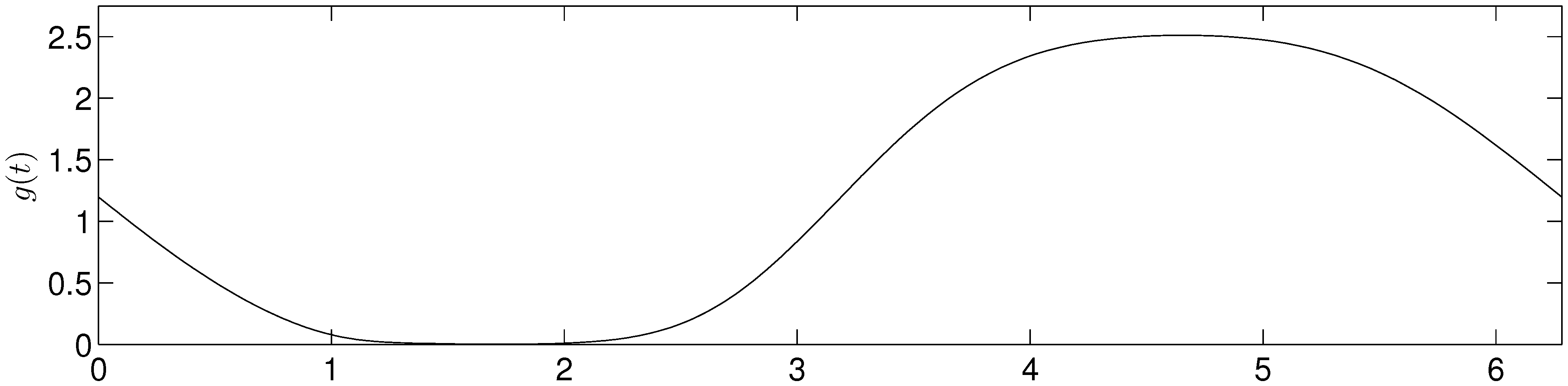Figure 2 shows the MFC over a period of a rotor oscillation in the case of a PCB with non-zero slip length. The MFC follows the path of a distorted negative sine curve, which is effectively constant and of very small magntiude between $t=1.32$ and $t=2.05$, with $g_{min}=4.97\times {10}^{-4}$. Physical dimensions of the the bearing corresponding to the result in Figure 2 are; ${\widehat{h}}_0=2\times {10}^{-4}$ m, ${\widehat{r}}_0=0.1$ m, ${\widehat{r}}_I=0.02$ m, , $\Delta \widehat{P}={10}^5$ Pa, $\widehat{\Omega }=228.21$s${}^{-1}$ and amplitude of rotor oscillation $1.8\times {10}^{-4}$. Considering an oil film with $\widehat{\rho }=800$Kgm${}^{-3}$ and $\mu ={10}^{-1}$Kgm${}^{-1}$s${}^{-1}$ gives the associated radial Reynolds number $Re=0.8$, radial velocity $\widehat{U}=0.5$ms${}^{-1}$, $R{e}^{*}=2.08\times {10}^3$ and speed parameter $\lambda =1$.

Figure 2. Minimum face clearance (MFC) over a period of rotor oscillation in the case of a PCB $\beta =0.2$ with slip length $l_s=0.29$ and amplitude of rotor oscillation $\epsilon =1.4$ with $g_{min}=4.97\times {10}^{-4}$; $a=0.2$, $\sigma =1$, $\lambda =1$, $\alpha =1$, $K_z=10$ and $D_a=1$.

Figure 2. Minimum face clearance (MFC) over a period of rotor oscillation in the case of a PCB $\beta =0.2$ with slip length $l_s=0.29$ and amplitude of rotor oscillation $\epsilon =1.4$ with $g_{min}=4.97\times {10}^{-4}$; $a=0.2$, $\sigma =1$, $\lambda =1$, $\alpha =1$, $K_z=10$ and $D_a=1$.

Table 1 shows the value of the slip length parameter when $g_{min}$ reaches a prescribed tolerance of decreasing magnitude $1\times {10}^{-3}\ge g_{tol}\ge 0$ in the case of a PCB and NCB with increasing amplitude of rotor oscillations, the smallest of which is close to where contact first occurs. Increasing the amplitude of rotor oscillations gives lower values of slip length for a given prescribed tolerance. The slip length values increase for decreasing prescribed tolerances, with tolerances $g_{tol}=1\times {10}^{-5}$ and $g_{tol}=0$ having effectively the same values; the former is significantly more straightforward to compute requiring typically only one run of the code opposed to multiple runs of the code with decreasing step size in $g_{min}$ for the later. A numerical approximation of face contact is adopted, when $g_{min}$ becomes less than a prescribed tolerance taken in this case as $g_{tol}=1\times {10}^{-5}$.

Table 1. Values of slip length for a given tolerance $0.001\ge g_{tol}\ge 0$ in the case of a PCB $\beta =0.2$ and NCB $\beta =-0.2$ for increasing values of amplitude of rotor oscillations $1.25\le \epsilon \le 1.60$ and $1.12\le \epsilon \le 1.60$, respectively; $a=0.2$, $\sigma =1$, $\lambda =1$, $\alpha =1$, $K_z=10$ and $D_a=1$.

		$g_{tol}=1\times {10}^{-3}$	$g_{tol}=1\times {10}^{-4}$	$g_{tol}=1\times {10}^{-5}$	$g_{tol}=0$
	$\epsilon =1.25$	2.20	2.34	2.35	2.35
$\beta =0.2$	$\epsilon =1.40$	0.283	0.295	0.296	0.296
	$\epsilon =1.60$	0.0542	0.0568	0.0570	0.0570
	$\epsilon =1.12$	2.39	2.58	2.60	2.60
$\beta =-0.2$	$\epsilon =1.30$	0.835	0.877	0.822	0.822
	$\epsilon =1.60$	0.0802	0.0877	0.0887	0.0887

Table 1. Values of slip length for a given tolerance $0.001\ge g_{tol}\ge 0$ in the case of a PCB $\beta =0.2$ and NCB $\beta =-0.2$ for increasing values of amplitude of rotor oscillations $1.25\le \epsilon \le 1.60$ and $1.12\le \epsilon \le 1.60$, respectively; $a=0.2$, $\sigma =1$, $\lambda =1$, $\alpha =1$, $K_z=10$ and $D_a=1$.

		$g_{tol}=1\times {10}^{-3}$	$g_{tol}=1\times {10}^{-4}$	$g_{tol}=1\times {10}^{-5}$	$g_{tol}=0$
	$\epsilon =1.25$	2.20	2.34	2.35	2.35
$\beta =0.2$	$\epsilon =1.40$	0.283	0.295	0.296	0.296
	$\epsilon =1.60$	0.0542	0.0568	0.0570	0.0570
	$\epsilon =1.12$	2.39	2.58	2.60	2.60
$\beta =-0.2$	$\epsilon =1.30$	0.835	0.877	0.822	0.822
	$\epsilon =1.60$	0.0802	0.0877	0.0887	0.0887

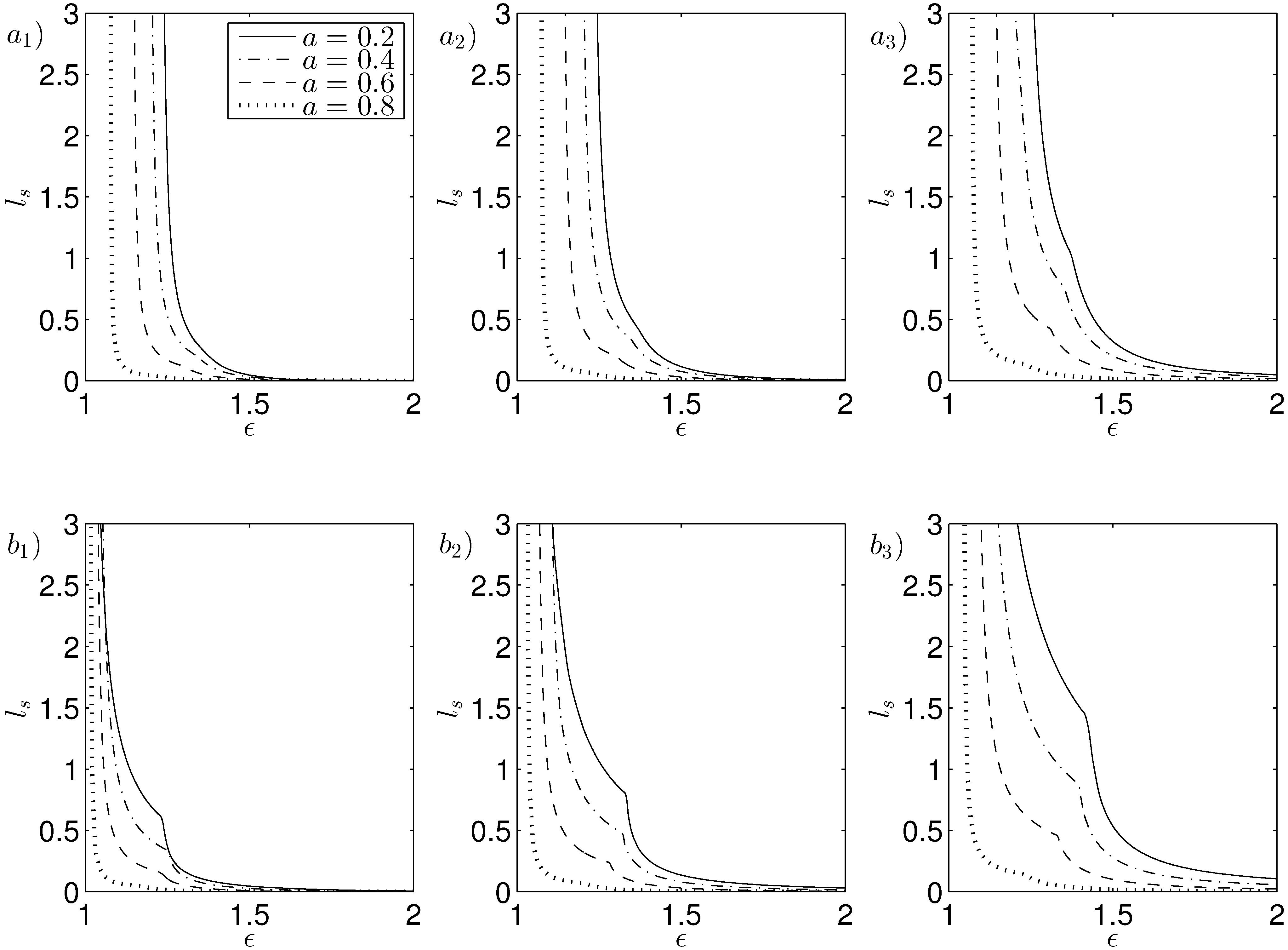
To compute the probability of contact, the values of the slip length and amplitude of rotor oscillations where contact first occurs are evaluated as shown in Figure 3. Configurations of a PCB and NCB, in the case of decreasing annulus and angle, are examined where face contact initially occurs for values of the slip length and amplitude of rotor oscillations on the curve in Figure 3. For parameter choices of slip length and amplitude of rotor oscillations above the curve, face contact occurs but a fluid film is maintained between the bearing faces for parameter choices under the curve. In the cases considered, for decreasing bearing width $0.8\ge (1-a)\ge 0.2$ face contact first occurs at lower values of amplitude of rotor oscillations for a given slip length, with the exception of a NCB with sufficiently large angle and slip length. Decreasing the coning angle of the rotor gives contact first occurring at larger values of slip length and amplitude of rotor oscillations. The contact curves exhibit non-smooth behaviour which is more distinct in a NCB than a PCB. The existence of this feature has been verified by using values of the slip length and amplitude of rotor oscillations close to the contact curve in the stroboscopic map solver, resulting in solutions of $g_{min}$ tending to the contact tolerance $g_{tol}=1\times {10}^{-5}$, and thus to the current contact curve. Analogous contact plots are produced for slip length against amplitude of rotor oscillations for a PCB and NCB with decreasing angle and increasing speed parameter in the case of a wide and narrow annulus. These results will be used to calculated the probability of contact during the parameter study. From a bearing design aspect, if the fluid gap becomes very small the tapered surfaces need to be limited to a small angle.

Figure 3. Contact plots of slip length against amplitude of rotor oscillations in the case of (a) PCB and (b) NCB with angle (1) $\mid \beta \mid =0.3$, (2) $\mid \beta \mid =0.2$ and (3) $\mid \beta \mid =0.1$ with decreasing annulus $0.8\ge (1-a)\ge 0.2$; $\lambda =1$, $\alpha =1$, $K_z=10$, $\sigma =1$ and $D_a=1$.

Figure 3. Contact plots of slip length against amplitude of rotor oscillations in the case of (a) PCB and (b) NCB with angle (1) $\mid \beta \mid =0.3$, (2) $\mid \beta \mid =0.2$ and (3) $\mid \beta \mid =0.1$ with decreasing annulus $0.8\ge (1-a)\ge 0.2$; $\lambda =1$, $\alpha =1$, $K_z=10$, $\sigma =1$ and $D_a=1$.

3. Uncertainty in Slip Length

Initially the slip length parameter is considered as a random variable reflecting the typical lack of knowledge of its precise value and the resulting uncertainty on the magnitude of $g_{min}$ is determined. Taking a constant slip length along the surface of the rotor and stator whose value is not known with certainty, a subjective interpretation of probability is used to model this lack of knowledge. Using the method of derived distributions, the corresponding effect of variability in the slip length parameter can be exactly determined, when it is expressed as a random variable. To incorporate that the slip length is always positive, a truncated log-normal probability density function (pdf) distribution is used providing a non-negative value with possible value ranging from the magnitude of bearing surface roughness to the order of the film thickness, or larger according to the nature of the fluid and solid material.

The truncated log-normal pdf and cumulative distribution function (CDF) used for the slip length are given by

$$\begin{array}{c}\hfill f_{L_s}(l_s;{\mu }_{l_s},{\sigma }_{l_s},3)=\frac{{\tilde{f}}_{L_s}(l_s;{\mu }_{l_s},{\sigma }_{l_s})}{{\tilde{F}}_{L_s}(3;{\mu }_{l_s},{\sigma }_{l_s})}\text{and}{F}_{L_s}(l_s;{\mu }_{l_s},{\sigma }_{l_s},3)=\frac{{\tilde{F}}_{L_s}(l_s;{\mu }_{l_s},{\sigma }_{l_s})}{{\tilde{F}}_{L_s}(3;{\mu }_{l_s},{\sigma }_{l_s})}\end{array}$$

(29)

in terms of the untruncated pdf, ${\tilde{f}}_{L_s}$ and CDF, ${\tilde{F}}_{L_s}$, with mean ${\mu }_{l_s}$ and standard deviation ${\sigma }_{l_s}$. The untruncated log-normal CDF is defined in terms of the untruncated pdf by

$$\begin{array}{ccc}\hfill {\tilde{F}}_{L_s}(l_s;{\mu }_{l_s},{\sigma }_{l_s})& =& \underset{-\infty }{\overset{l_s}{\int }}{\tilde{f}}_{L_s}(t;{\mu }_{l_s},{\sigma }_{l_s})dt\hfill \\ & =& \frac{1}{\sqrt{2\pi }\sqrt{ln\left(1+\frac{{\sigma }_{l_s}^2}{{\mu }_{l_s}^2}\right)}}\underset{-\infty }{\overset{l_s}{\int }}\frac{1}{t}exp\left(\frac{-{\left(lnt-ln\left(\frac{{\mu }_{l_s}^2}{\sqrt{{\sigma }_{l_s}^2+{\mu }_{l_s}^2}}\right)\right)}^2}{2{\sqrt{ln\left(1+\frac{{\sigma }_{l_s}^2}{{\mu }_{l_s}^2}\right)}}^2}\right)dt\hfill \end{array}$$

(30)

For example when a carbon surface is used, which is known to have large value of slip length, the log-normal distribution is right truncation at $l_s=3$. Initially the average value and standard deviation will be taken as $0.1$, with the effect of alternative average values and standard deviations examined later.

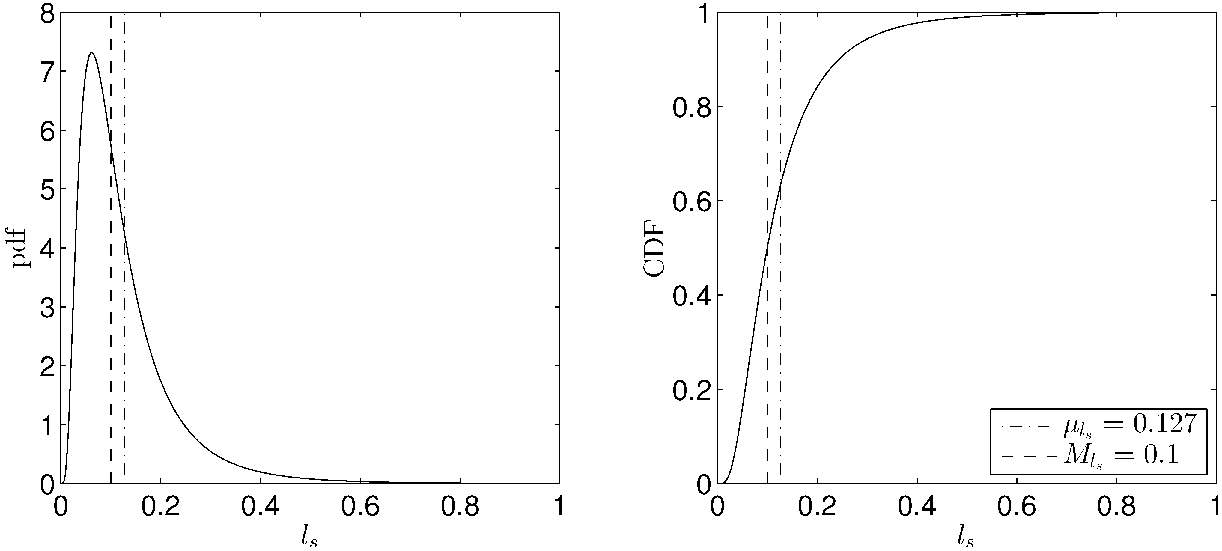
Truncating the distribution however may lead to the specified mean not being representative of the average value of the distribution. Figure 4 shows the pdf and CDF with standard deviation ${\sigma }_{l_s}=0.1$ and effective median M at the desired average value, $M_{l_s}=0.1$, requiring the prescribed mean to be larger than the average value; ${\mu }_{l_s}=0.127$. The discrepancy between the effective median and prescribed mean increases as the standard deviation increases. Therefore throughout this work the prescribed mean of the distribution is such that the effective median is representative of the desired average value of the slip length.

Figure 4. Probability density function (pdf) and cumulative distribution function (CDF) of slip length with standard deviation ${\sigma }_{l_s}=0.1$ and $M_{l_s}$$=0.1$, with prescribed mean ${\mu }_{l_s}=0.127$.

Figure 4. Probability density function (pdf) and cumulative distribution function (CDF) of slip length with standard deviation ${\sigma }_{l_s}=0.1$ and $M_{l_s}$$=0.1$, with prescribed mean ${\mu }_{l_s}=0.127$.

Describing the slip length by a pdf allows the corresponding pdf of $g_{min}$ to be found using the change of variables, $f_{Gmin}\left(g_{min}\right)=\mid \partial l_s/\partial g_{min}\mid f_{L_s}\left(l_s\right)$, where the derivative is found from the stroboscopic map solver. The CDF of $g_{min}$ can also be calculated, giving the probability $g_{min}$ is less than or equal to a given tolerance, thus the probability of contact is given when $g_{min}\le 1\text{x}{10}^{-5}$. To calculate the CDF of $g_{min}$, the set of deterministic slip lengths giving $g_{min}$ less than or equal to each possible specified value is required; namely $A_{l_s{g}_{min}}=\{L_s:{\chi }_{\epsilon }\left(l_s\right)\le g_{min}\}$. In this set, ${\chi }_{\epsilon }$ denotes the deterministic relation between the slip length and $g_{min}$ which can be found for different amplitude of rotor oscillations ε using the mathematical model. The untruncated CDF of the minimum face clearance is calculated by

$$\begin{array}{ccc}\hfill {\tilde{F}}_{G_{min}}\left(g_{min}\right)& =& P(G_{min}\le g_{min})=P({\chi }_{\epsilon }\left(L_s\right)\le g_{min})=P\left(\{L_s:{\chi }_{\epsilon }\left(l_s\right)\le g_{min}\}\right)\hfill \\ & =& {\int }_{A_{l_s{g}_{min}}}{\tilde{f}}_{L_s}(l_s;{\mu }_{l_s},{\sigma }_{l_s})d{l}_s\hfill \end{array}$$

(31)

Thus the truncated CDF for $g_{min}$ is given by

$$\begin{array}{c}\hfill F_{G_{min}}\left(g_{min}\right)=\frac{{\int }_{A_{l_s{g}_{min}}}{\tilde{f}}_{L_s}(l_s;{\mu }_{l_s},{\sigma }_{l_s})d{l}_s}{{\tilde{F}}_{L_s}(3;{\mu }_{l_s},{\sigma }_{l_s})}\end{array}$$

(32)

using the untruncated functions given in (30).

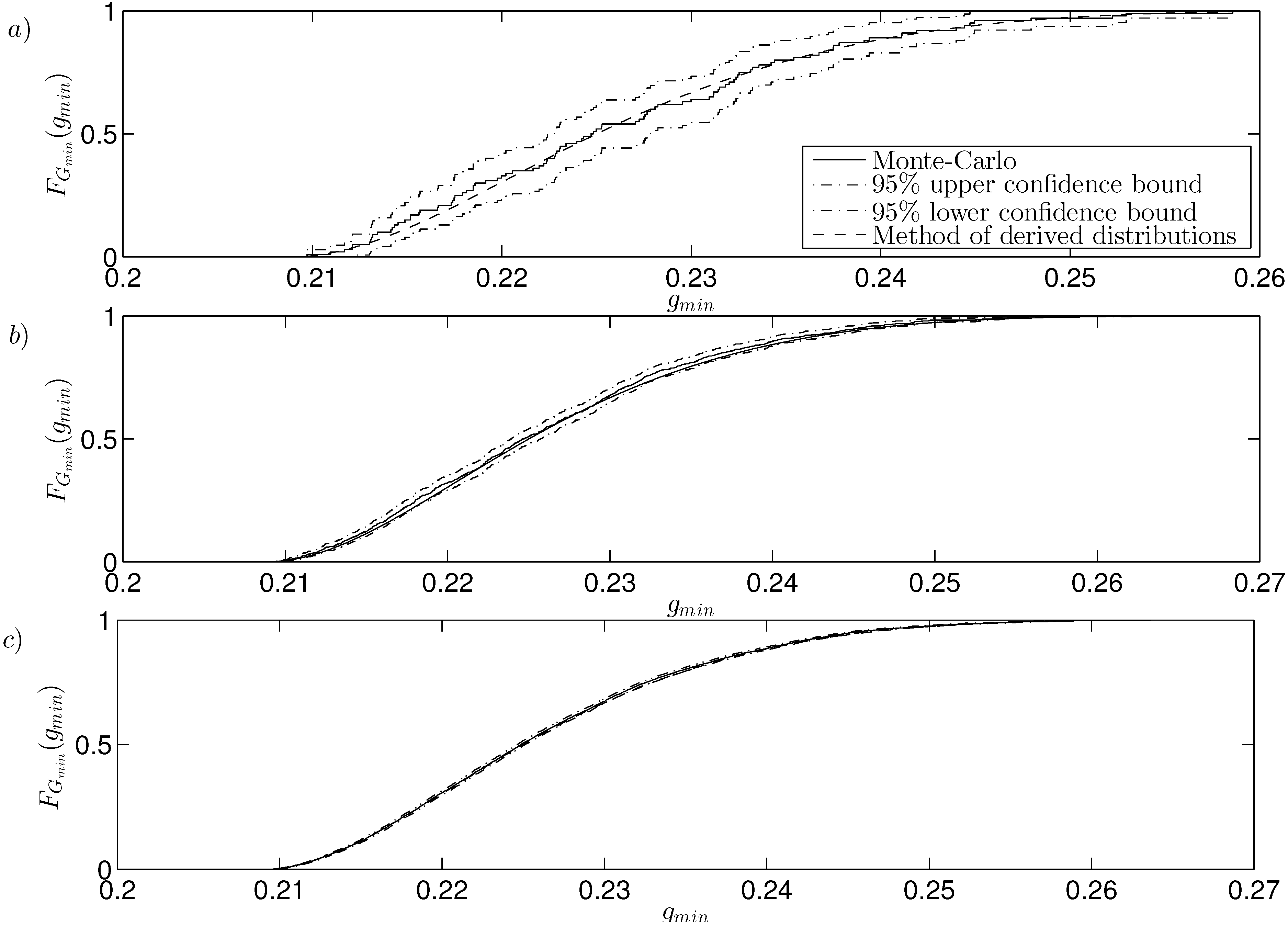
Comparison of the CDF of $g_{min}$ obtained from the Monte Carlo method and by using the method of derived distributions is given in Figure 5. In this case the Monte Carlo method is run with an increasing number of steps and the slip length values are taken at random from the truncated distribution. Obtaining the values of $g_{min}$ for each chosen slip length via the stroboscopic map solver allows the CDF and $95\%$ upper and lower confidence bounds to be computed. The CDF computed by the method of derived distributions uses Equations (32) and the deterministic relation between the slip length and $g_{min}$ to find the set of values $A_{l_s{g}_{min}}$. Increasing the number of steps used in the Monte Carlo method gives the CDF converging to the result computed via the method of derived distributions. The Monte Carlo method was computationally more expensive, requiring $10,000$ steps to achieve the same level of accuracy as the method of derived distributions. For further calculations the method of derived distributions was used to produce subsequent results. The bearing configuration in this case gives $g_{min}\ge 0.210$, giving a zero probability of contact.

Figure 5. CDF of $g_{min}$ calculated using the method of derived distributions and a Monte-Carlo method with (a) 100, (b) 1000 and (c) $10,000$ steps for the case of a PCB $\beta =0.2$ with wide annulus and slip length distribution with median $M_{l_s}$$=0.1$, standard deviation ${\sigma }_{l_s}=0.1$; $a=0.2$, $\sigma =1$, $\lambda =1$, $\alpha =1$, $K_z=10$, $D_a=1$.

Figure 5. CDF of $g_{min}$ calculated using the method of derived distributions and a Monte-Carlo method with (a) 100, (b) 1000 and (c) $10,000$ steps for the case of a PCB $\beta =0.2$ with wide annulus and slip length distribution with median $M_{l_s}$$=0.1$, standard deviation ${\sigma }_{l_s}=0.1$; $a=0.2$, $\sigma =1$, $\lambda =1$, $\alpha =1$, $K_z=10$, $D_a=1$.

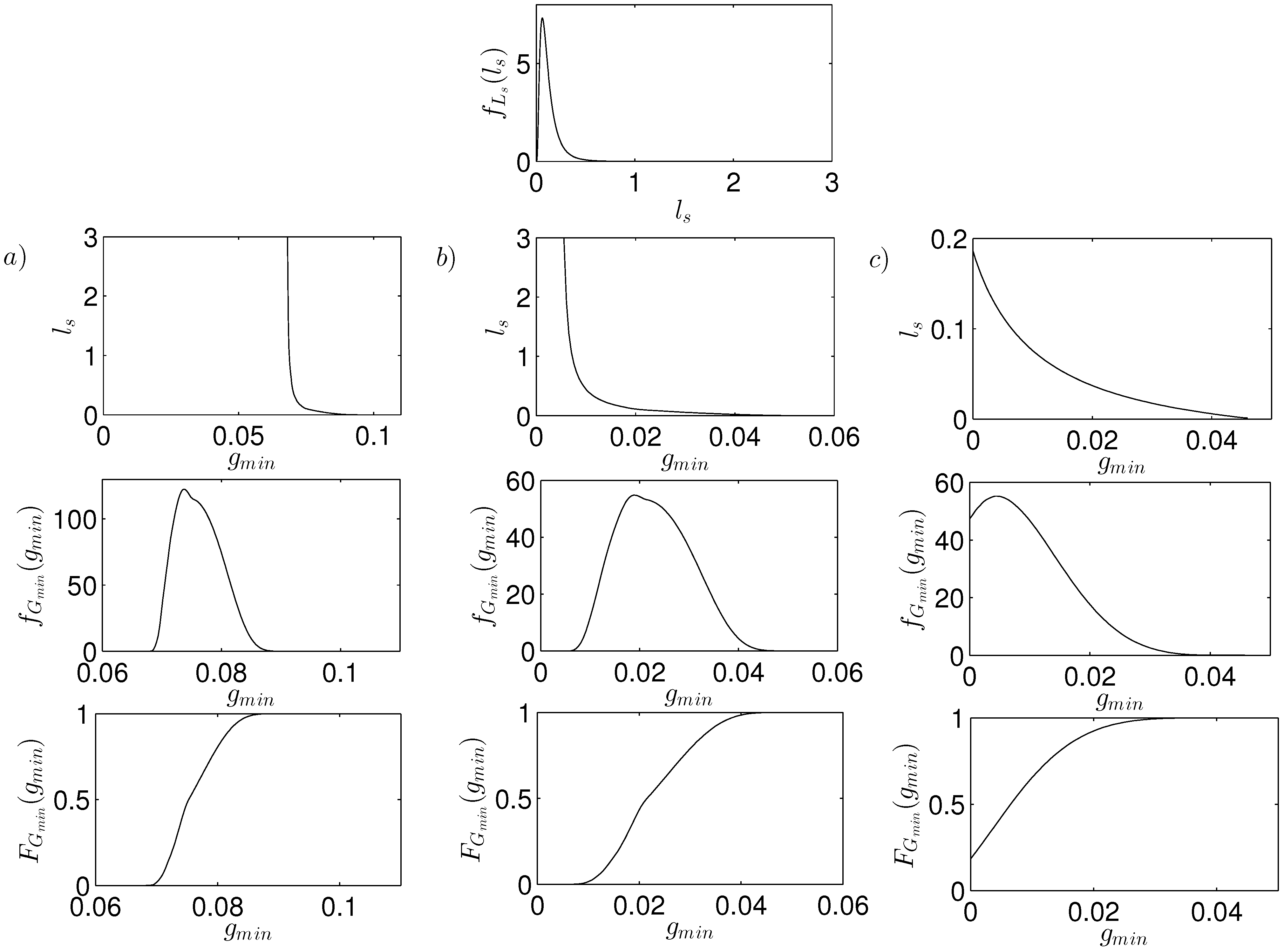
Figure 6 shows the deterministic relationship between the slip length and $g_{min}$ and the corresponding pdf and CDF of $g_{min}$ for increasing amplitude of rotor oscillations in the case of a PCB and slip length distribution; median $M_{l_s}$$=0.1$, standard deviation ${\sigma }_{l_s}=0.1$. The deterministic results show the amplitude of rotor oscillations taking $\epsilon =1.00$ and $1.07$ with increasing slip length have $g_{min}$ decreasing asymptotically to a constant value. However for larger amplitude of rotor oscillations $\epsilon =1.10$, $g_{min}$ decreases until face contact at $l_s=0.186$. The pdf of $g_{min}$ shows smaller values are likely to occur as the amplitude of rotor oscillations increase, with the CDF showing the smallest value of $g_{min}$ with probably 1 decreases as the amplitude of rotor oscillations increase. The probability of contact is given when the CDF intercepts the y-axis, giving P(contact) $=0$ for $\epsilon =1.00$ and $1.07$ but P(contact) $=0.185$ for $\epsilon =1.10$.

Figure 6. Probability density function (pdf) of slip length, deterministic relationship between $g_{min}$ and slip length, pdf of $g_{min}$ and CDF of $g_{min}$ for increasing amplitude of rotor oscillations (a) $\epsilon =1.00$, (b) $\epsilon =1.07$ and (c) $\epsilon =1.10$ in the case of a PCB $\beta =0.2$ with narrow annulus and slip length distribution with median $M_{l_s}$$=0.1$, standard deviation ${\sigma }_{l_s}=0.1$; $a=0.8$, $\sigma =1$, $\lambda =1$, $\alpha =1$, $K_z=10$, $D_a=1$.

Figure 6. Probability density function (pdf) of slip length, deterministic relationship between $g_{min}$ and slip length, pdf of $g_{min}$ and CDF of $g_{min}$ for increasing amplitude of rotor oscillations (a) $\epsilon =1.00$, (b) $\epsilon =1.07$ and (c) $\epsilon =1.10$ in the case of a PCB $\beta =0.2$ with narrow annulus and slip length distribution with median $M_{l_s}$$=0.1$, standard deviation ${\sigma }_{l_s}=0.1$; $a=0.8$, $\sigma =1$, $\lambda =1$, $\alpha =1$, $K_z=10$, $D_a=1$.

For parameter studies of the probability of contact, it is convenient to compute the probability of contact directly using

$$\begin{array}{c}\hfill P\text{(contact)}=\frac{{\int }_{A_{l_s{g}_{tol}}}{\tilde{f}}_{L_s}(l_s;{\mu }_{l_s},{\sigma }_{l_s})d{l}_s}{{\tilde{F}}_{L_s}(3;{\mu }_{l_s},{\sigma }_{l_s})}\end{array}$$

(33)

where $A_{l_s{g}_{tol}}=\{L_s:{\chi }_{\epsilon }\left(l_s\right)\le g_{tol}\}$ is the set of discrete values of the slip length parameter which give face contact for different deterministic values of the amplitude of rotor oscillations. Therefore the probability of contact is given as a function of the amplitude of rotor oscillations. The set $A_{l_s{g}_{tol}}$ can be found using the deterministic contact curves in Figure 3 and analogous plots for increasing speed parameter in the case of wide and narrow annuli.

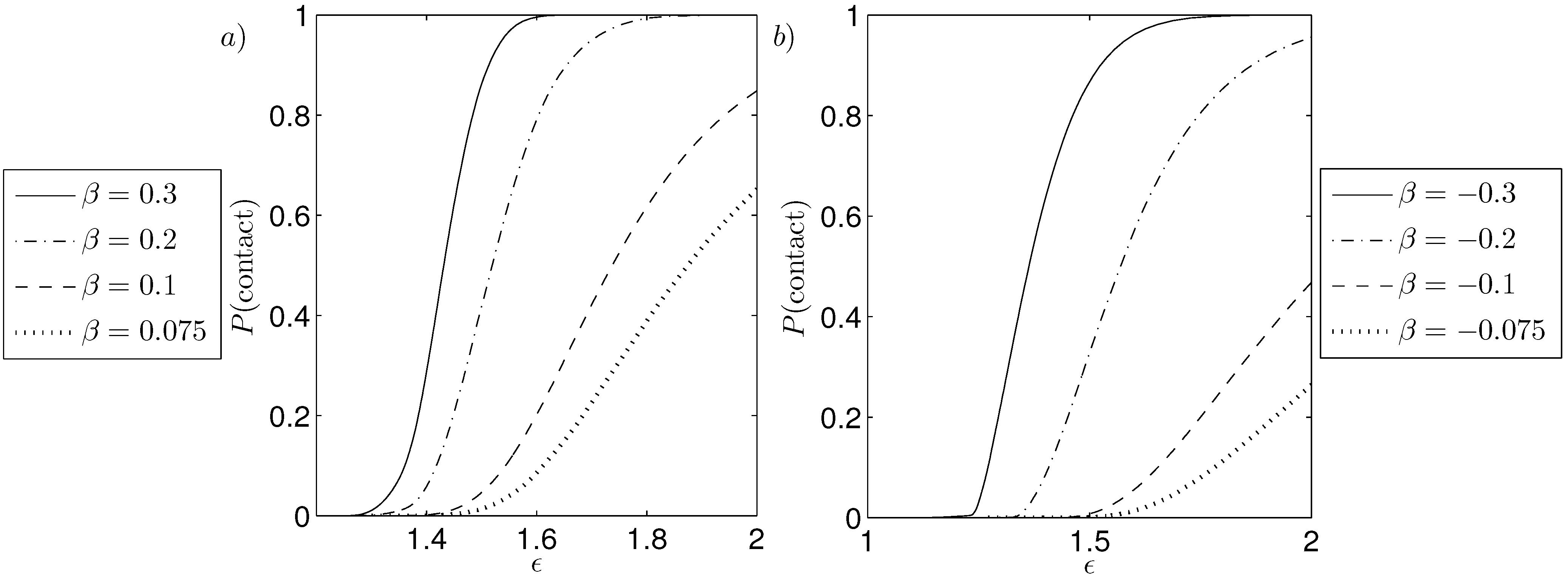
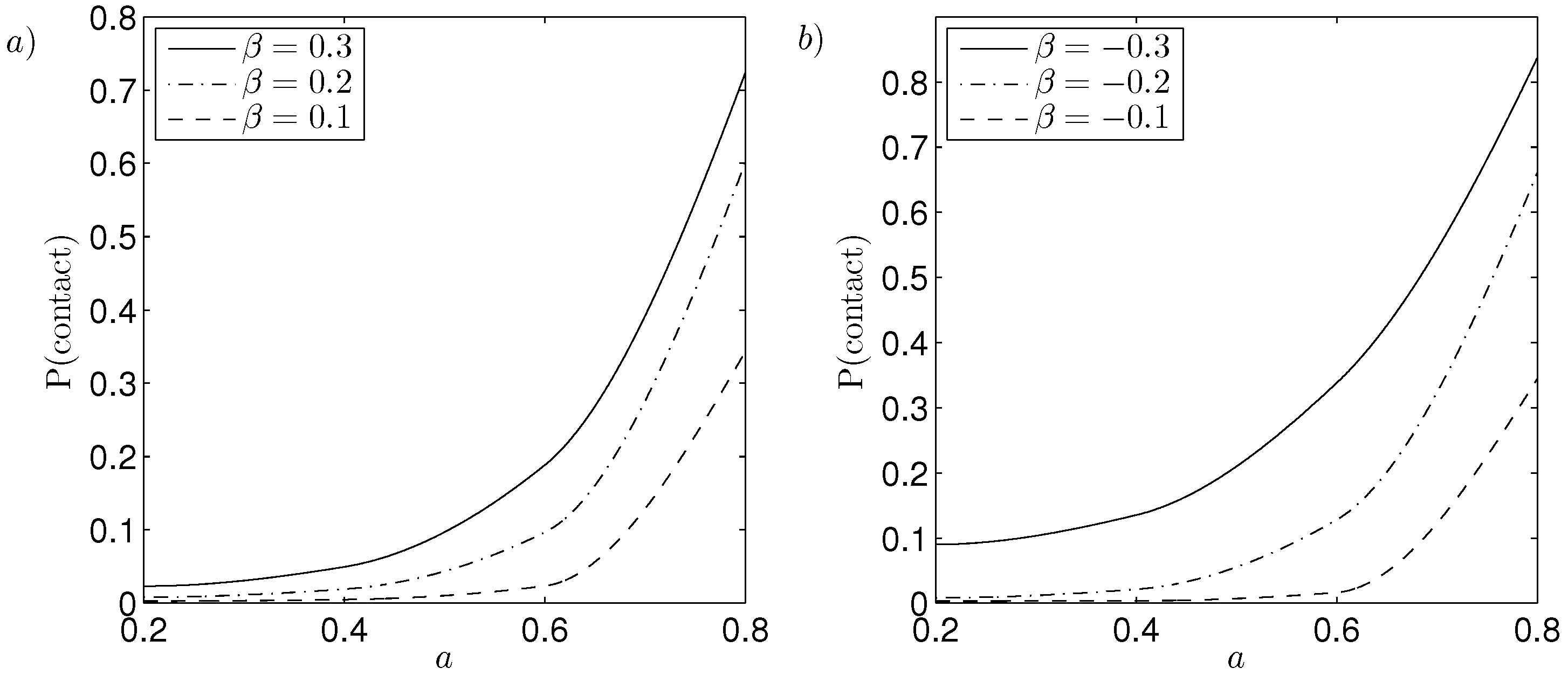
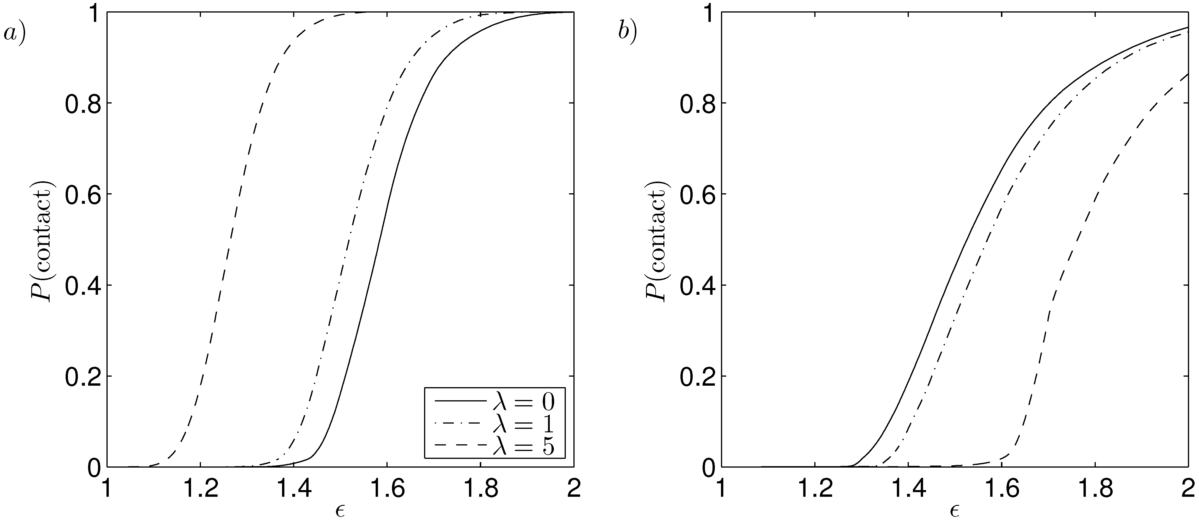
The probability of contact against amplitude of rotor oscillations for increasing speed parameter in the case of a PCB and NCB is shown in Figure 7. In the case of a PCB increasing the amplitude of rotor oscillations increases the probability of contact, with the probability of contact increasing from 0 to 1 over a small range of amplitude of rotor oscillations. For a given value of amplitude of rotor oscillations the probability of contact increases for an increasing speed parameter due to a PCB being externally pressurised and the effects of inertia overcoming the differential pressure to decrease $g_{min}$ and therefore increase the probability of contact. On the other hand a NCB has P(contact) remaining less than 1, see Figure 7b, although it becomes large at the upper limit of amplitude of rotor oscillations $\epsilon =2$. Increasing the speed parameter reduces the probability of contact for a given amplitude of rotor oscillations as a NCB is internally pressurised giving the effects of inertia coinciding with the differential pressure to increase $g_{min}$ and thus decrease the probability of contact.

Figure 7. Probability of contact against amplitude of rotor oscillations for increasing speed parameter $0\le \lambda \le 5$ in the case of (a) PCB; $\beta =0.2$ and (b) NCB $\beta =-0.2$ with wide annulus and slip length distribution median $M_{l_s}=0.1$, standard deviation ${\sigma }_{l_s}=0.1$; $a=0.2$, $\sigma =1$, $\alpha =1$, $K_z=10$, $D_a=1$.

Figure 7. Probability of contact against amplitude of rotor oscillations for increasing speed parameter $0\le \lambda \le 5$ in the case of (a) PCB; $\beta =0.2$ and (b) NCB $\beta =-0.2$ with wide annulus and slip length distribution median $M_{l_s}=0.1$, standard deviation ${\sigma }_{l_s}=0.1$; $a=0.2$, $\sigma =1$, $\alpha =1$, $K_z=10$, $D_a=1$.

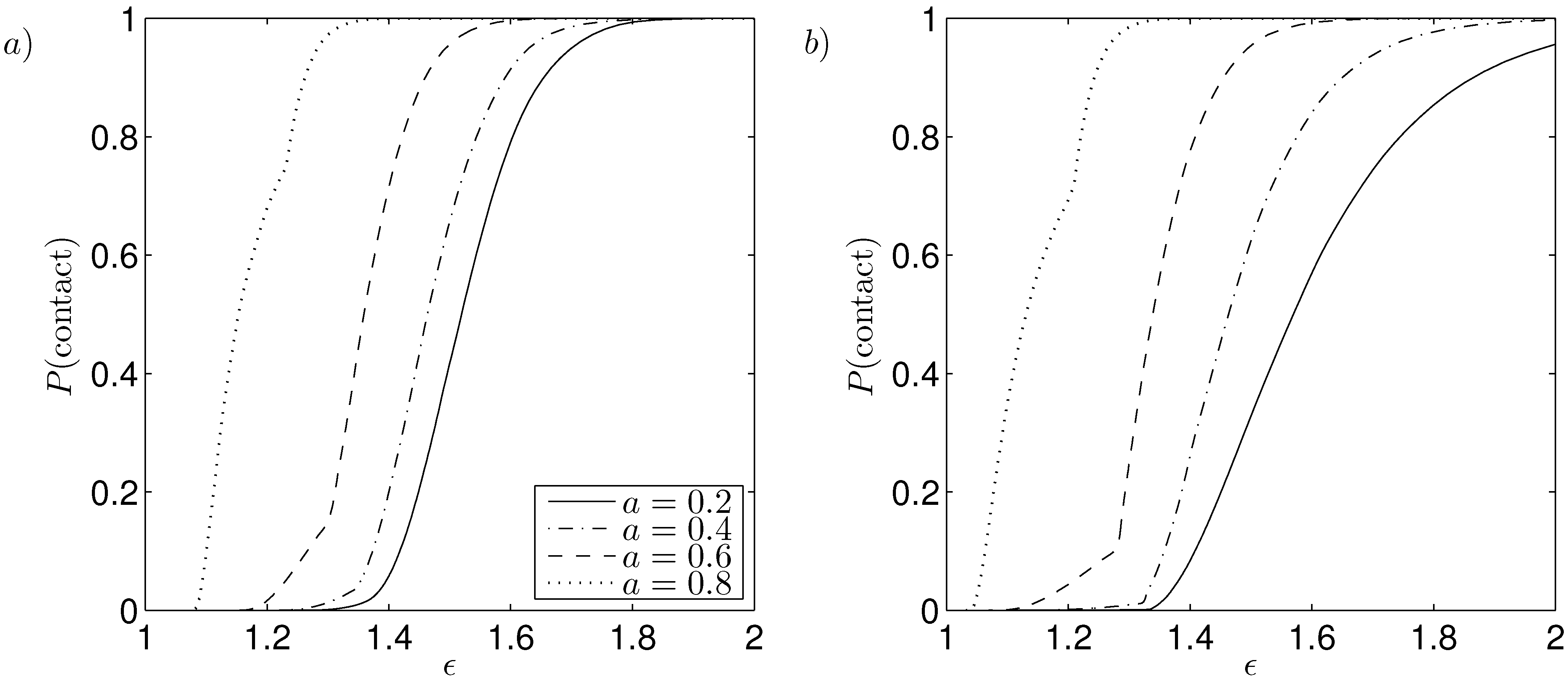
The probability of contact against amplitude of rotor oscillations for a PCB and NCB in the case of decreasing angle is given in Figure 8, where increasing the amplitude of rotor oscillations increases the probability of contact. Decreasing the coning angle in a PCB and NCB decreases the probability of contact for a given amplitude of rotor oscillations, tending to the limit of a parallel bearing which has zero probability of contact under the conditions considered in this work. It is important to observe that the non-contact condition found for a parallel bearing is due to the inclusion of inertial effect not considered in classical lubrication theory. Under non-pressurisation conditions and zero inertial effect the fluid stiffness (16) is zero and consequently contact is expected under extreme conditions. A PCB has zero probability of contact for larger amplitude of rotor oscillations than a NCB, but larger probabilities of contact for amplitude of rotor oscillations larger than a given value which is less than $\epsilon =1.50$ for all the cases considered. The non-smooth behaviour in these plots is due to the discontinuity in the deterministic solutions as shown in Figure 3.

Figure 8. Probability of contact for (a) PCB and (b) NCB with decreasing coning angle with wide annulus and slip length distribution median $M_{l_s}$$=0.1$, standard deviation ${\sigma }_{l_s}=0.1$, ${\mu }_{l_s}=0.127$; $a=0.2$, $\lambda =1$, $\sigma =1$, $\alpha =1$, $K_z=10$, $D_a=1$.

Figure 8. Probability of contact for (a) PCB and (b) NCB with decreasing coning angle with wide annulus and slip length distribution median $M_{l_s}$$=0.1$, standard deviation ${\sigma }_{l_s}=0.1$, ${\mu }_{l_s}=0.127$; $a=0.2$, $\lambda =1$, $\sigma =1$, $\alpha =1$, $K_z=10$, $D_a=1$.

The effect of decreasing bearing width on the probability of contact is shown in Figure 9 over increasing amplitude of rotor oscillations for a PCB and NCB, where increasing the amplitude of rotor oscillations increases the probability of contact. Deceasing the bearing width gives an increased probability of contact for a given amplitude of rotor oscillations, with a PCB having larger increases than a NCB. In the case of a narrow annulus $a=0.8$, a NCB has a larger probability of contact than a PCB for a given amplitude of rotor oscillations, whereas other bearing widths considered have a PCB or NCB having a larger probability of contact depending upon the magnitude of amplitude of rotor oscillations.

Figure 9. Probability of contact for (a) PCB; $\beta =0.2$ and (b) NCB; $\beta =-0.2$ with decreasing annulus $0.2\le a\le 0.8$ with slip length distribution median $M_{l_s}$$=0.1$, standard deviation ${\sigma }_{l_s}=0.1$, ${\mu }_{l_s}=0.127$; $\lambda =1$, $\sigma =1$, $\alpha =1$, $K_z=10$, $D_a=1$.

Figure 9. Probability of contact for (a) PCB; $\beta =0.2$ and (b) NCB; $\beta =-0.2$ with decreasing annulus $0.2\le a\le 0.8$ with slip length distribution median $M_{l_s}$$=0.1$, standard deviation ${\sigma }_{l_s}=0.1$, ${\mu }_{l_s}=0.127$; $\lambda =1$, $\sigma =1$, $\alpha =1$, $K_z=10$, $D_a=1$.

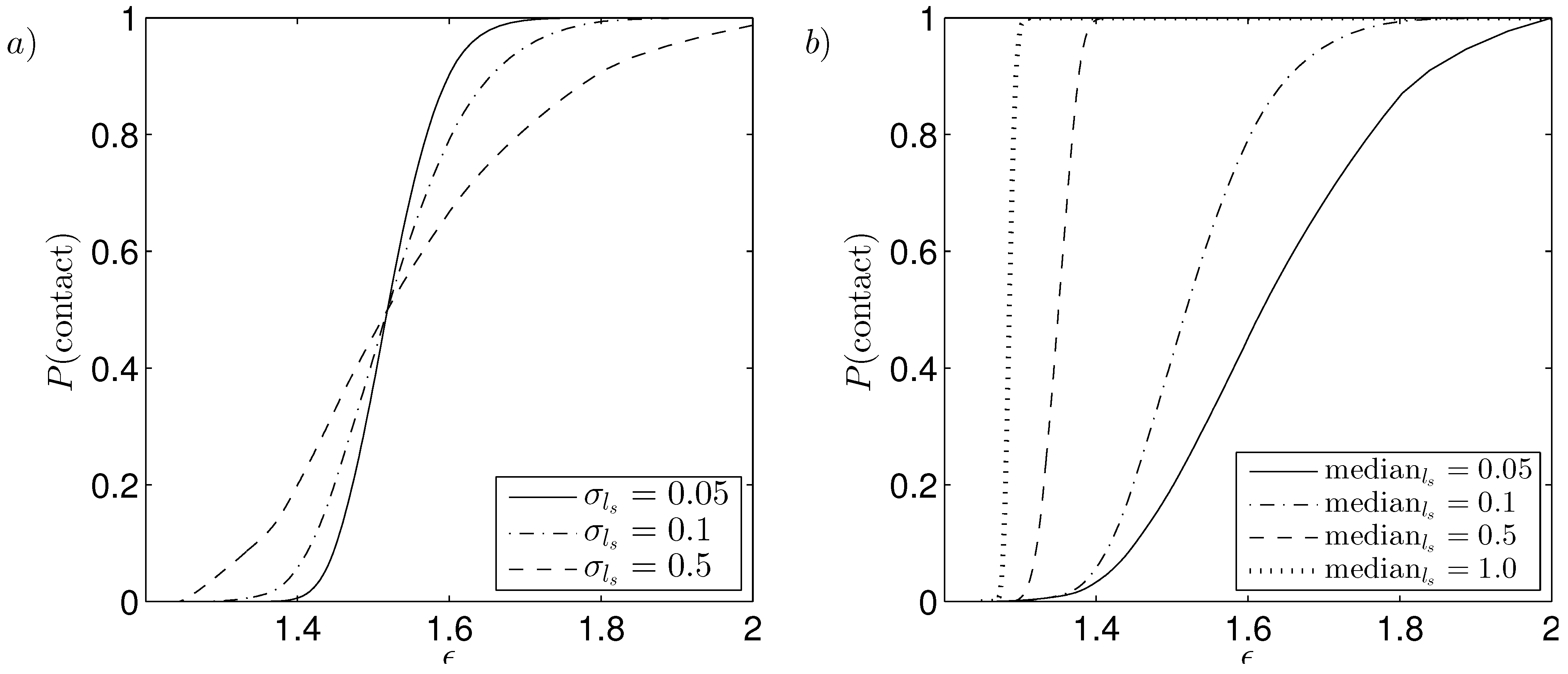
The effect of the probabilistic parameters on the probability of contact is examined by considering the case of a fixed median with increasing standard deviation and increasing median with fixed standard deviation as shown in Figure 10 for a PCB. Increasing the standard deviation of the slip length causes the probability of contact to increase for a given amplitude of rotor oscillations in the case of $\epsilon <{\epsilon }_c$, but to decrease otherwise, with critical value ${\epsilon }_c=1.52$ where the probability of contact curves intersect in Figure 10a. This situation arises as increasing the standard deviation gives slip lengths over a greater range, with $\epsilon <{\epsilon }_c$ leading to an increase in the probability of contact. Whereas for $\epsilon >{\epsilon }_c$ the range of slip lengths which do not give contact increases and thus decreases the probability of contact. The effect of slip lengths with increased median is shown in Figure 10b where a larger probability of contact for a given amplitude of rotor oscillation, with the transition of probability of contact increasing over a shorter range of amplitude of rotor oscillations.

Figure 10. Probability of contact for a wide PCB with (a) fixed median $M_{l_s}=0.1$, increasing standard deviation $0.05\le {\sigma }_{l_s}\le 0.5$ and (b) increasing median $0.05\le M_{l_s}$$\le 1.0$, fixed standard deviation ${\sigma }_{l_s}=0.1$; $\beta =0.2$, $a=0.2$, $\sigma =1$, $\lambda =1$, $\alpha =1$, $K_z=10$ and $D_a=1$.

Figure 10. Probability of contact for a wide PCB with (a) fixed median $M_{l_s}=0.1$, increasing standard deviation $0.05\le {\sigma }_{l_s}\le 0.5$ and (b) increasing median $0.05\le M_{l_s}$$\le 1.0$, fixed standard deviation ${\sigma }_{l_s}=0.1$; $\beta =0.2$, $a=0.2$, $\sigma =1$, $\lambda =1$, $\alpha =1$, $K_z=10$ and $D_a=1$.

Corresponding plots for a NCB give a similar trend to a PCB with a small magnitude change. For sufficiently large amplitude of rotor oscillations a NCB has larger probability of contact than a PCB, otherwise the reverse situation is true.

4. Uncertainty in Slip Length and Amplitude of Rotor Oscillations

An additional source of uncertainty in bearing operation is from the axial oscillations of the rotor which are subject to a random excitation. A simplified case where oscillations are considered periodic with random amplitude is given by Hou et al. [32]. For the current study the oscillations are considered periodic with constant amplitude, but the value is not known with certainty, allowing an exact solution for a two parameter random input problem to be obtained. Expressing the slip length and amplitude of rotor oscillations as random variables, and using the deterministic results for the relation between the values of slip length and amplitude of rotor oscillations at contact (for example Figure 3), allows the probability of contact to be calculated.

The rotor oscillations are described by $h_r=\epsilon sint$, where the amplitude ε is defined as a random variable instead of a fixed parameter. Following the approach adapted in the previous section the slip length is described by a truncated log-normal pdf. The amplitude of the rotor oscillations is modelled by a double truncated normal function, to include the expectation of little skewing. Truncation of the normal distribution is required to ensure the amplitude of rotor oscillations is non-negative and, as in realistic applications, the amplitude of rotor oscillations is restricted; in the results shown the upper limit is set at $\epsilon =2$ which is twice the equilibrium gap $g=1$. Initially the average value of the amplitude of rotor oscillations is taken as $\epsilon =1.2$ to reflect extreme conditions, with the amplitude of rotor oscillations larger then the equilibrium gap. The standard deviation is taken as ${\sigma }_{\epsilon }=0.1$, with the effects of changes in the average value and standard deviation examined later.

The truncated normal pdf and CDF for the amplitude of the rotor oscillations are given by

$$\begin{array}{ccc}\hfill f_E(\epsilon ;{\mu }_{\epsilon },{\sigma }_{\epsilon },0,2)& =& \frac{{\tilde{f}}_E(\epsilon ;{\mu }_{\epsilon },{\sigma }_{\epsilon })}{{\tilde{F}}_E(2;{\mu }_{\epsilon },{\sigma }_{\epsilon })-{\tilde{F}}_E(0;{\mu }_{\epsilon },{\sigma }_{\epsilon })}\hfill \end{array}$$

(34)

$$\begin{array}{ccc}\hfill F_E(\epsilon ;{\mu }_{\epsilon },{\sigma }_{\epsilon },0,2)& =& \frac{{\tilde{F}}_E(\epsilon ;{\mu }_{\epsilon },{\sigma }_{\epsilon })-{\tilde{F}}_E(0;{\mu }_{\epsilon },{\sigma }_{\epsilon })}{{\tilde{F}}_E(2;{\mu }_{\epsilon },{\sigma }_{\epsilon })-{\tilde{F}}_E(0;{\mu }_{\epsilon },{\sigma }_{\epsilon })}\hfill \end{array}$$

with mean ${\mu }_{\epsilon }$ and standard deviation ${\sigma }_{\epsilon }$. The untruncated pdf, ${\tilde{f}}_E$ and CDF, ${\tilde{F}}_E$ are defined by

$$\begin{array}{ccc}\hfill {\tilde{F}}_E(\epsilon ;{\mu }_{\epsilon },{\sigma }_{\epsilon })& =& {\int }_{-\infty }^{\epsilon }{\tilde{f}}_E(t;{\mu }_{\epsilon },{\sigma }_{\epsilon })dt=\frac{1}{{\sigma }_{\epsilon }\sqrt{2\pi }}\underset{-\infty }{\overset{\epsilon }{\int }}exp\left(\frac{-{(t-{\mu }_{\epsilon })}^2}{2{\sigma }_{\epsilon }^2}\right)dt\hfill \end{array}$$

(35)

It is assumed the amplitude of rotor oscillations and slip length random variables are statistically independent, giving the joint pdf as the product of their marginal pdf $f_{E,L_s}(\epsilon ,l_s)=f_E\left(\epsilon \right)f_{L_s}\left(l_s\right)$. To compute the probability of contact the deterministic contact curves are used, as given in Figure 3, to find the set of amplitude of rotor oscillations $A_{\epsilon g_{tol}}=\{E:G_{min}\le g_{tol}\}$ and slip lengths $A_{l_s{g}_{tol}}=\{L_s:G_{min}\le g_{tol}\}$ which give $g_{min}$ less than or equal to the contact tolerance $g_{tol}=1\times {10}^{-5}$. The probability of contact is computed numerically using

$$\begin{array}{ccc}\hfill P(G_{min}\le 0)& =& P\left(\{L_s:G_{min}\le g_{tol}\}\right)P\left(\{E:G_{min}\le g_{tol}\}\right)\hfill \\ & =& {\int }_{A_{l_s{g}_{tol}}}{f}_{L_s}\left(l_s\right)d{l}_s{\int }_{A_{\epsilon g_{tol}}}{f}_E\left(\epsilon \right)d\epsilon \hfill \end{array}$$

(36)

whose value is represented by the area above the contact curve in the probability space. The probability of contact is computed numerically using Matlab.

The probability of contact for differing bearing geometries in a PCB and NCB are shown in Figure 11 with decreasing coning angle and bearing width. Decreasing the bearing width $(1-a)$ increases the probability of contact, with greater increases as the bearing width decreases. Decreasing the coning angle in a PCB and NCB reduces the probability of contact for all given bearing widths. A PCB and NCB with small coning angle $\mid \beta \mid =0.1$ have similar probabilities of contact, whereas for increasing coning angles a PCB has consistently lower probability of contact than a NCB.

Figure 11. Probability of contact against bearing width for (a) PCB and (b) NCB with decreasing angle; $M_{\epsilon }=1.2$, ${\sigma }_{\epsilon }=0.1$, $M_{l_s}=0.1$, ${\sigma }_{l_s}=0.1$, $\sigma =1$, $\lambda =1$, $\alpha =1$, $K_z=10$ and $D_a=1$.

Figure 11. Probability of contact against bearing width for (a) PCB and (b) NCB with decreasing angle; $M_{\epsilon }=1.2$, ${\sigma }_{\epsilon }=0.1$, $M_{l_s}=0.1$, ${\sigma }_{l_s}=0.1$, $\sigma =1$, $\lambda =1$, $\alpha =1$, $K_z=10$ and $D_a=1$.

Table 2 shows the probability of contact for a PCB and NCB in the case of a wide ($a=0.2$) and narrow ($a=0.8$) annulus with increasing speed parameter. Results show increasing the coning angle consistently increases the probability of contact and the probability of contact is greater in a bearing with a narrow annulus compared to a wide annulus. Increasing the speed parameter has an opposing effect between the two bearing types, a PCB has the probability of contact increasing whereas a NCB has a decreased probability of contact. As a PCB is externally pressurised, the effects of inertia overcome the differential pressure giving contact at a smaller value of $l_s$ and therefore a larger probability of contact as the speed parameter increases. Whereas a NCB is internally pressurised giving the effects of inertia coinciding with the differential pressure to give contact at a larger value of $l_s$ as the speed parameter increases and thus a smaller probability of contact. A NCB has a larger probability of contact than a PCB, with the exception of a sufficiently large speed parameter as indicated by the shaded region in Table 2. In these cases, the contact curves for a PCB sit below those for a NCB, with contact at smaller values of slip lengths and amplitude of rotor oscillations.

Table 2. Probability of contact for a NCB ($\beta <0$) and PCB ($\beta >0$) in the case of a wide $a=0.2$ and narrow $a=0.8$ annulus with increasing speed parameter $0\le \lambda \le 5$; $M_{\epsilon }=1.2$, ${\sigma }_{\epsilon }=0.1$, $M_{l_s}=0.1$, ${\sigma }_{l_s}=0.1$, $\sigma =1$, $K_z=10$, $\alpha =1$ and $D_a=1$.

	wide, a = 0.2			narrow, a = 0.8
	λ = 0	λ = 1	λ = 5	λ = 0	λ = 1	λ = 5
$\beta =0.1$	$0.00162$	$0.00281$	$0.0414$	$0.328$	$0.343$	$0.409$
$\beta =0.2$	$0.00288$	$0.00819$	$0.291$	$0.598$	$0.602$	$0.665$
$\beta =0.3$	$0.00624$	$0.0231$	$0.609$	$0.709$	$0.724$	$0.781$
$\beta =-0.1$	$0.00337$	$0.00319$	$0.00264$	$0.357$	$0.344$	$0.292$
$\beta =-0.2$	$0.0184$	$0.00826$	$0.00326$	$0.680$	$0.671$	$0.627$
$\beta =-0.3$	$0.179$	$0.0902$	$0.00381$	$0.852$	$0.836$	$0.785$

Table 2. Probability of contact for a NCB ($\beta <0$) and PCB ($\beta >0$) in the case of a wide $a=0.2$ and narrow $a=0.8$ annulus with increasing speed parameter $0\le \lambda \le 5$; $M_{\epsilon }=1.2$, ${\sigma }_{\epsilon }=0.1$, $M_{l_s}=0.1$, ${\sigma }_{l_s}=0.1$, $\sigma =1$, $K_z=10$, $\alpha =1$ and $D_a=1$.

	wide, a = 0.2			narrow, a = 0.8
	λ = 0	λ = 1	λ = 5	λ = 0	λ = 1	λ = 5
$\beta =0.1$	$0.00162$	$0.00281$	$0.0414$	$0.328$	$0.343$	$0.409$
$\beta =0.2$	$0.00288$	$0.00819$	$0.291$	$0.598$	$0.602$	$0.665$
$\beta =0.3$	$0.00624$	$0.0231$	$0.609$	$0.709$	$0.724$	$0.781$
$\beta =-0.1$	$0.00337$	$0.00319$	$0.00264$	$0.357$	$0.344$	$0.292$
$\beta =-0.2$	$0.0184$	$0.00826$	$0.00326$	$0.680$	$0.671$	$0.627$
$\beta =-0.3$	$0.179$	$0.0902$	$0.00381$	$0.852$	$0.836$	$0.785$

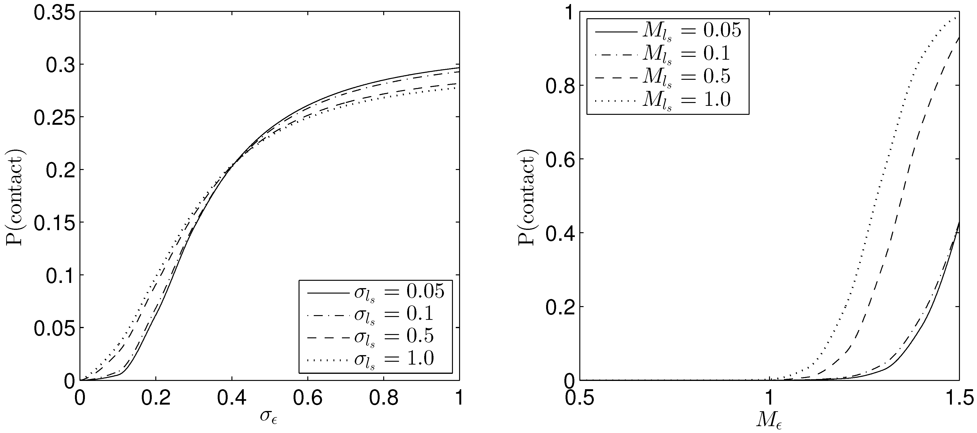
To evaluate the effect of values associated with the distribution parameters, the probability of contact is examined for increasing standard deviations with fixed medians and increasing medians with fixed standard deviations. Figure 12 shows the probability of contact against the standard deviation of the amplitude of rotor oscillations with increasing standard deviation of the slip length and against median of amplitude of rotor oscillations with increasing median of the slip length in the case of a PCB. Increasing the standard deviation of the amplitude of rotor oscillations increases the probability of contact. The effect of increasing the standard deviation of the slip length however depends on the size of the standard deviation of the amplitude of rotor oscillations with respect to a critical value ${\sigma }_{\epsilon c}$, given as the value where the probability of contact curves intersect in Figure 12a. Increasing the standard deviation of the slip length gives the probability of contact increasing (decreasing) for standard deviations of the amplitude of rotor oscillations below (above) the critical value ${\sigma }_{\epsilon c}=0.424$, due to more values of the slip length giving contact (no contact) being included. Results in Figure 12b show increasing the median value of the amplitude of rotor oscillations gives negligible probability of contact until $\epsilon \le 1$. Increasing the median of the slip length increases the probability of contact.

Figure 12. Probability of contact against (a) standard deviation of the amplitude of rotor oscillations with increasing standard deviation of the slip length $0\le {\sigma }_{l_s}\le 1$; $M_{\epsilon }=1.2$, $M_{l_s}=0.1$ and (b) median of the amplitude of rotor oscillations with increasing median of the slip length $0.1\le M\le 1.0$; ${\sigma }_{\epsilon }=0.1$, ${\sigma }_{l_s}=0.1$ in the case of a PCB with wide annulus; $a=0.2$, $\sigma =1$, $\lambda =1$, $\alpha =1$, $K_z=10$ and $D_a=1$.

Figure 12. Probability of contact against (a) standard deviation of the amplitude of rotor oscillations with increasing standard deviation of the slip length $0\le {\sigma }_{l_s}\le 1$; $M_{\epsilon }=1.2$, $M_{l_s}=0.1$ and (b) median of the amplitude of rotor oscillations with increasing median of the slip length $0.1\le M\le 1.0$; ${\sigma }_{\epsilon }=0.1$, ${\sigma }_{l_s}=0.1$ in the case of a PCB with wide annulus; $a=0.2$, $\sigma =1$, $\lambda =1$, $\alpha =1$, $K_z=10$ and $D_a=1$.

Corresponding plots for a NCB show the probability of contact for increasing standard deviation of the slip length and amplitude of rotor oscillations has a similar trend but with a decrease in magnitude for a given choice of probabilistic parameters. In the case of increasing median of the slip length and amplitude of rotor oscillations a NCB has a similar trend to a PCB but with a small magnitude shift. For the cases considered in Figure 12; small slip length medians, $M_{l_s}=0.05$ and $0.1$ give a larger probability of contact in a PCB than a NCB, effectively the same for median $M_{l_s}=0.5$ and for larger slip length median $M_{l_s}=1.0$ a NCB has larger probability of contact than a PCB.

5. Conclusions and Summary

A deterministic mathematical model is extended for a high speed pressurised thin film bearing containing a rigid coned rotor with a slip length boundary condition imposed on the bearing faces. The axial motion of the stator is modelled as a spring-mass-damper system to investigate a fully coupled unsteady bearing when subject to uncertainty in amplitude of rotor oscillations and slip length parameter. In an initial deterministic analysis of the film the Reynolds equation and stator equation are given in terms of the time dependent minimum face clearance, allowing explicit analytic expressions for the pressure field, force on the stator and a nonlinear second-order non-autonomous ordinary differential modified stator equation to be derived. A stroboscopic map solver is implemented to find periodic solutions. The performance of two coned bearing configurations, a PCB and NCB are considered under external and internal pressurisation, respectively and examined under extreme operating conditions.

Recognising the realistic implications of uncertainty in the model parameter values the slip length parameter is taken as a random variable with prescribed mean and standard deviation together with similar attributes for the amplitude of the axial rotor oscillations. The value of the prescribed mean is such that the effective median of the random parameter is representative of the required average value. The deterministic mathematical model is used to find the relation between the slip length and $g_{min}$, allowing the pdf of $g_{min}$ to be computed. The CDF of $g_{min}$ is found via the method of derived distributions from which the probability of contact can be found; a numerical approximation of face contact is used to significantly reduce the computational requirement without loss of accuracy. The probability of contact is determined directly for the parameter studies.

A detailed study is provided to evaluate the effects of uncertainty in values of the slip length parameter on potential bearing geometries associated with coning angle, bearing width and rotational speed. Results show an increase in the probability of contact as the amplitude of rotor oscillations increase, a wide bearing has a lower probability of contact than a narrow bearing and a small angle giving a reduced probability of contact compared to a large angle. Increasing the speed parameter causes a decreased probability of contact for a NCB but increased probability in a PCB due to the inertial effects overcoming the differential pressure effects. Examining the effects of different distribution parameters shows increasing the median of the slip length increases the probability of contact and increasing the standard deviation for an amplitude of rotor oscillation below a critical value ${\epsilon }_c$ increases the probability of contact whereas for amplitude of rotor oscillation $\epsilon >{\epsilon }_c$ decreases the probability of contact.

To reflect operational bearing conditions the slip length and amplitude of rotor oscillations parameters are considered as random variables with a prescribed mean and standard deviation and the method of derived distributions is used to calculate the probability of contact. Results show decreasing the bearing width and increasing the coning angle increases the probability of contact. Increasing the speed parameter gives the probability of contact increasing in a PCB but decreasing in a NCB. Increasing the slip length standard deviation causes the probability of contact to increase for standard deviations of the amplitude of rotor oscillations below a critical value ${\sigma }_{\epsilon }<{\sigma }_{\epsilon c}$, but decrease for ${\sigma }_{\epsilon }>{\sigma }_{\epsilon c}$. Increasing the median of the slip length and amplitude of rotor oscillations increases the probability of contact.