1. Introduction
There exists a wide range of works on friction analysis for assemblies with lubricated contacts. A number of them are reviewed in order to derive relevant requirements on a modeling technique to be applied in particular for internal combustion engines (ICEs).
Coy [
1] reviews approaches to model friction and wear in engines. It is demonstrated that detailed rheological models are requested, where the effects of pressure, temperature and shear rate need to be taken into account, if realistic friction and wear data are to be developed. The author states furthermore that if elastic effects are to be incorporated, then the full set of coupled equations governing the flow of the lubricant taking proper account of the moving parts of the geometry must be analyzed. Using static solvers and thus neglecting squeeze lubrication effects, is not appropriate, as squeeze effects are most important at small oil film thicknesses. Taylor and Coy [
2] compare results, which are obtained by different institutions applying different simulation models for different engines. In particular, a 1.8-liter, a two-liter and a five-liter engine are compared at different operating conditions. Comparing only the total friction power loss results shows large differences. These underline the need of accurate and stable simulation models for this kind of application. The authors note the importance of a realistic viscometry (
i.e., variations of viscosity with pressure, temperature and shear rate) consideration. In particular, the authors state that the actual power loss distribution and the overall power loss are very sensitive to the temperatures assumed in the engine components, since lubricant viscosity varies strongly with temperature. A further very detailed work has been written by Taylor [
3]. The author investigates the connecting rod bearing loads. A short bearing approximation considering squeeze effects is applied for that purpose. The author notes that, for low speeds, the connecting rod loads are often dominated by the combustion gas pressure. However, as engine speed increases, inertia effects begin to dominate, which makes an appropriate consideration of these effects necessary. Further works have been reported by Schwaderlapp
et al. [
4], where a more theoretical case of a mass less engine is presented as well as by Daniels and Braun [
5], where transient friction contributions by individual engine components during a simulated warm up are simulated as well as by Mufti and Priest [
6].
Summarizing the discussed works yields the following requests on a model in order to predict friction power loss in radial slider bearings of an ICE accurately:
All structural components need to be modeled as three-dimensional and flexible considering inertia effects.
Detailed rheological models, which are able to represent different kinds of oil, like for instance multi-grade oils, and their additives have to be provided. Lubricant properties, like viscosity, density, conductivity and heat capacity have to be considered with their dependencies related to temperature, pressure and shear rate.
The contact model has to consider hydrodynamic, mixed and boundary lubrication regimes, and therefore be able to compute pressure (hydrodynamic and asperity) and shear stresses (hydrodynamic and asperity) based on the dynamics of the clearance gap. Surface roughness has to be considered in the oil flow in terms of flow factors.
In order to guarantee realistic contact conditions, real contact surface profiles have to be considered. This implies considering the influence of, for instance, manufacturing and structural thermal deviation as well as wear profiles.
Effects of the oil supply have to be considered. Both the possibility of time dependent boundary conditions, a representation as fixed, and an oil supply network representation is required to consider the pressure and flow interaction between the main journal and connecting rod big end bearings.
The oil viscosity changes according to the lubricant temperature. Therefore, an exact determination of the local temperature distribution in the bearing is necessary, which requires the consideration of the thermal equations parallel to the hydrodynamic equations.
Due to the highly nonlinear interaction, a coupled simulation of components and contacts in time domain is needed.
2. Flexible Multi-Body System and Averaged Reynolds Equation
Offner [
9] presents a flexible multi-body approach, which considers the above listed requirements by dynamically simulating (
Figure 1) the combined torsion and bending vibrations of the component assembly. The approach is implemented in AVL EXCITE, [
10]. Allmaier
et al. [
7] and Priestner
et al. [
8] present works, of which simulation parts are based on [
9] and [
10], and which discuss a systematic validation of simulation results with experimental measurements.
The mathematical modeling of each flexible component, which will be called body in the further text, is based on a “Floating Frame of Reference Formulation”. Besides beam-mass models and structured models according to Parikyan
et al. [
13], the commonly used finite element models, for instance [
14], which may optionally be condensed, see Offner [
15], are used. Besides the excitation by gas and mass forces, the interaction between engine components as well as the non-linear behavior in the contacts between the component surfaces, shortly called joints, is considered. A detailed representation of these contacts is needed to predict the mechanical functionality, the structural excitation as well as to consider local phenomena, as for instance friction phenomena, in the contact itself. Oil film lubricated contacts play an important role. Radial and axial slider bearings as well as the piston cylinder liner contacts are typical oil film lubricated contacts, which need to be represented in a simulation model. The well-known Reynolds equation is the mathematical model, which is applied, when representing oil film lubricated contacts and which is solved on a finite volume grid. As boundary and mixed lubrication regimes are typical, an averaged Reynolds equation has to be applied. The equation computes hydrodynamic pressure in the clearance gap considering the shape of the clearance gap the amount of oil in the gap (fill rate and supply) and properties of the oil itself, as dynamic viscosity and density and flow conditions. The flow conditions are represented by flow factors. Patir and Cheng [
12] used pressure and shear flow factors as functions of surface roughness characteristics. Pressure flow factors
,
compare the average pressure flow of rough component surfaces to that of a smooth surfaces. Shear flow factors
represent the additional flow transport due to sliding of a rough component surface. These flow factors can be derived independently from the mean flow quantities obtained from numerical simulation of for instance a bearing with a randomly generated or measured surface roughness.
Furthermore, some contacts are not oil film lubricated at all, but nevertheless need a mathematical representation in the model. Examples are local areas in oil film lubricated contacts, where not enough oil support is available. For covering this, a dry contact needs to be applied. The contact equations compute fluid or dry pressure depending on the clearance gap between the body surfaces in contact and its first derivative with respect to time.
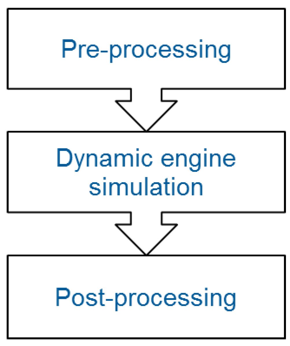
The approach consists of three basic workflow steps,
Figure 1. In a pre-processing step the setup of all bodies (e.g., engine block, crank shaft, connecting rods, pistons,
etc.) and all contacts between the bodies (e.g., main bearings, big end bearings,
etc.) of a model excitation load is done. Furthermore, operating conditions such as, for instance, gas load, engine speed and according initial conditions, have to be specified.
The non-linear model, which is set up in the pre-processing step, is solved in a time domain applying numerical time integration. A backward differentiation formula (BDF) is used for that purpose. Each time step is solved on an iterative basis solving both the equations of motion of all bodies of a model, Drab
et al. [
17], and the contact equations between certain contacting body surfaces. A Newton-Raphson procedure is applied for each contact, [
9]. Within each iteration, the clearance gap and its time derivative are interpolated from the coupled surface nodes of the two contacting bodies to the finite volume grid discretization, respectively, in a first step.
Based on the clearance gap geometry, dynamic fluid data, flow factors, etc., both the hydrodynamic and the asperity pressure but also tangential surface shear stress distributions are computed using the finite volume approach. Pressures and shear stresses are integrated to nodal forces (and moments in case of a beam model), which are again considered in the equation of motion of both connected bodies.
Obtained results can be investigated, compared and animated in a final post-processing step.
Based on this framework, a generic friction model for radial slider bearings, which is applied during the dynamic multi-body simulation, is derived in the following section.
Figure 1.
Overall workflow.
Figure 1.
Overall workflow.
3. Generic Friction Model for Radial Slider Bearings
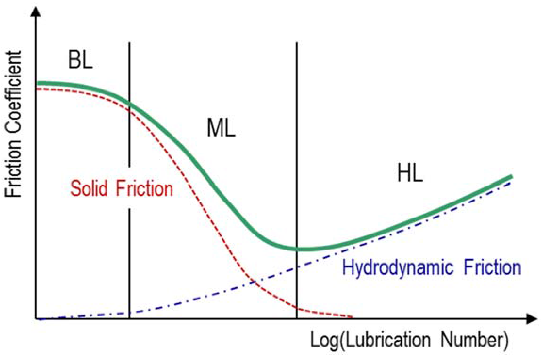
Radial slider bearings are exposed to a variety of different operating conditions in terms of loads, speeds and temperatures. The operating conditions, reflected as friction coefficient, may range depending on the lubrication number from purely hydrodynamic lubrication (HL) with a sufficiently thick oil film to mixed lubrication (ML) or even boundary lubrication (BL) with significant amounts of asperity contact (
Figure 2). The lubrication number in this figure is the typical non-dimensional speed defined by relative angular velocity, bearing load, lubricant viscosity and the bearing diameter as reference length.
In the case of hydrodynamic lubrication, friction depends on oil film formation, which again depends on the oil film viscosity, the dynamics of the clearance gap and the relative sliding velocity. In addition to hydrodynamic influences, friction depends in the case of mixed lubrication but in particular in the case of boundary lubrication also on solid contact properties. This requires an appropriate representation of shape and material properties of both contacting surfaces.
Figure 2.
Schematic representation of friction coefficient over lubrication number at boundary, mixed and hydrodynamic lubrication.
Figure 2.
Schematic representation of friction coefficient over lubrication number at boundary, mixed and hydrodynamic lubrication.
3.1. Methods
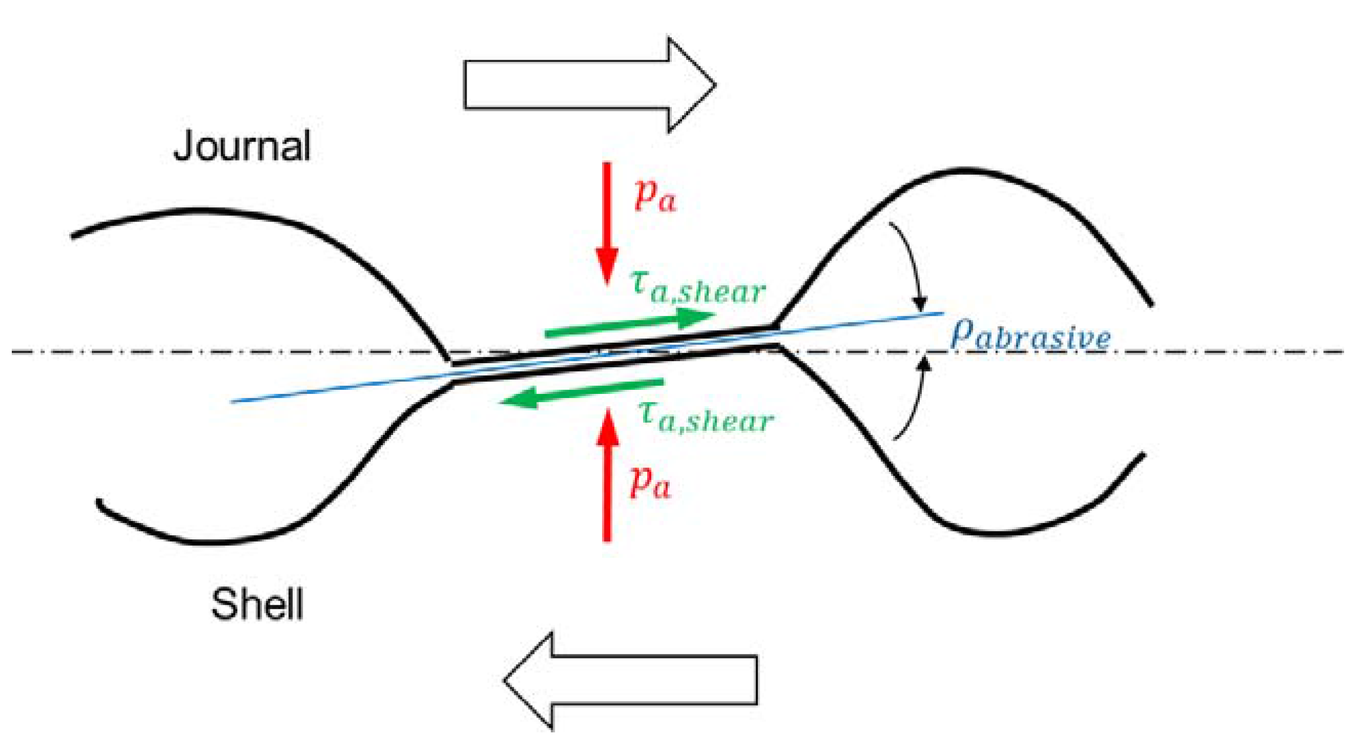
Surface friction forces are to be integrated from shear stresses, which act on the contacting body surfaces. Superimposed shear stress components from hydrodynamic and asperity contacts are considered for this purpose.
As Newtonian oil properties can be assumed, the shear stress formula of Newton [
10] can be used for evaluating the hydrodynamic shear stress. Similar to the approach used for mean oil flow, empirical shear stress factors are defined such that the mean hydrodynamic shear stress is given in terms of mean quantities, reading
Similar to the Reynolds equation, , and are the clearance gap height, the hydrodynamic pressure and the dynamic oil film viscosity. and are the velocities in sliding direction of the two contacting body surfaces journal and shell.
Equation (1) considers expressions for the mean shear stress and horizontal forces due to local pressure in rough contacts
and
.
and
are viscous shear stress tensors due to Poisseuille Couette flow. Similar to
,
is an additional term in the mean shear stress equations resulting from the combined effect of sliding and roughness. Due to the
effect, a rough surface experiences a smaller mean shear stress than the opposing smooth surface. The rough surface, however, experiences an additional horizontal force due to the local pressure acting in the sides of the asperities and valleys.
arises from averaging the sliding velocity component of the shear stress. It can be obtained through integration for any given frequency density of roughness heights. Similar to the pressure and shear flow factors, these flow factors can be identified by a separated analysis [
11], or can be taken from Patir and Cheng [
12].
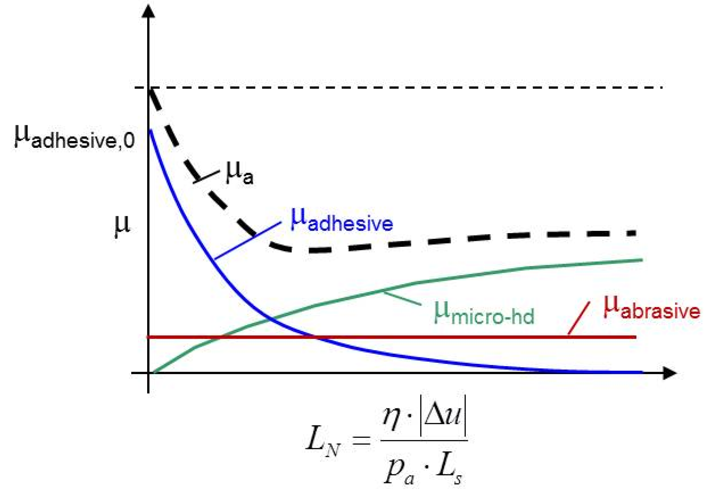
Since the yield stress varies with the instantaneous condition of the solid and surface layer properties in a complex manner, the mean asperity shear stress can be computed according Coulomb’s friction law by
where
is the asperity contact pressure. The dimensionless friction coefficient
is variable and considers the hydrodynamic surface separation in the microscopic scale for the surface roughness summit interaction as well as the transition into solid-to-solid contact due to adhesive forces (
Figure 3).
Figure 3.
Surface contact layer on journal and shell side.
Figure 3.
Surface contact layer on journal and shell side.
According to this, the coefficient can be subdivided into the sum of an abrasive
, a solid contact
and a micro-hydrodynamic
friction coefficient
is Coulomb’s friction coefficient for solid contacts at sticking condition and
is the asperity contact ratio. In addition to the dynamic viscosity
and the asperity pressure
, the lubrication number
considers the mean sliding velocity
.
is a reference length for the summit contact and reads
with an averaged summit density
, a mean contact radius
and the roughness orientation
.
The abrasive friction coefficient is depending on the shape of surface roughness texture and represents the constant part of the friction
vs. speed. The adhesive friction represents the specific shear stress limit relative to contact pressure at zero relative velocity. With increased lubrication, the percentage of solid-to-solid contact reduces according to the logarithmic function. On the other hand, it increases the percentage of the micro-hydrodynamic load carrying and, with it, the viscous shear stress in the asperity contact (
Figure 4).
Figure 4.
Asperity friction coefficient characteristic as the sum of the three friction components vs. lubrication number.
Figure 4.
Asperity friction coefficient characteristic as the sum of the three friction components vs. lubrication number.
The constants for one contact pair are “”, “” and “”, respectively. Beside the surface texture and surface material combinations, the oil additives also play a major rule. So-called friction reducer additives improve the micro-hydrodynamic pressure buildup. The coefficients have to be determined experimentally in tribometer tests.
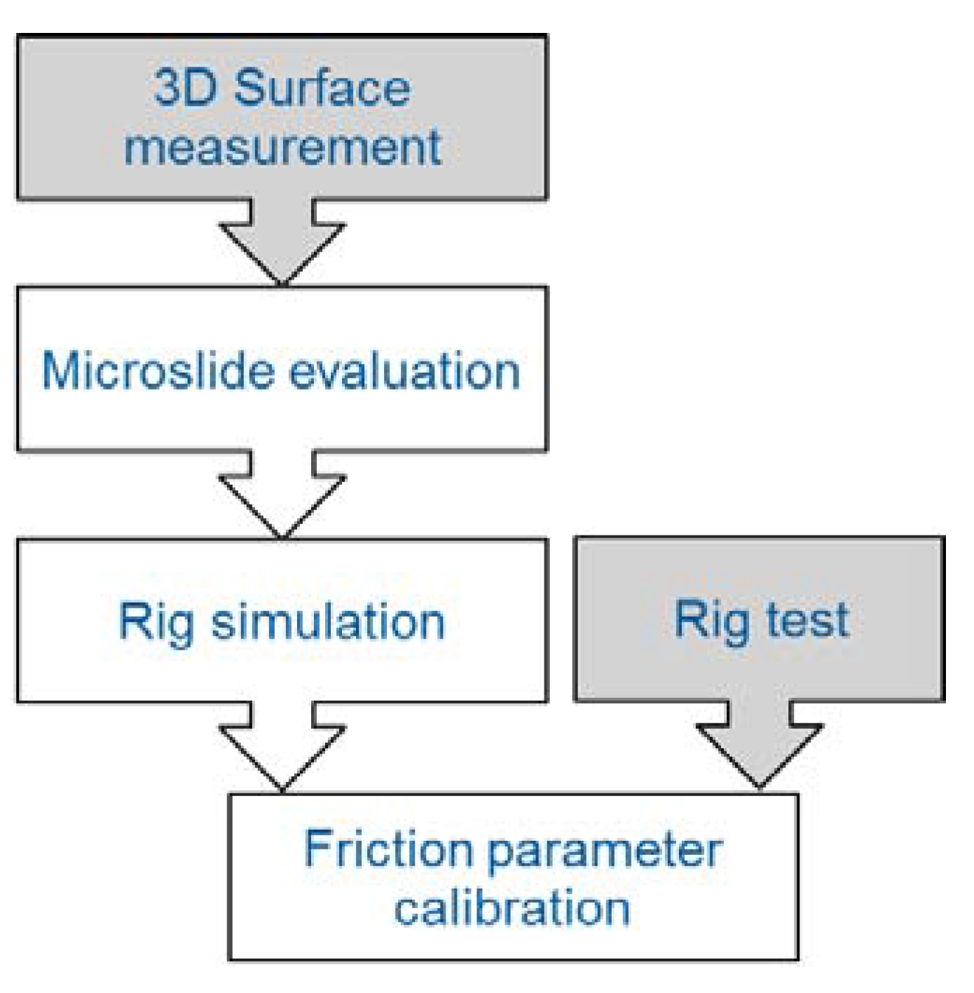
3.2. Parameter Identification Workflow
Figure 5 shows steps, which are required to identify friction parameters. These have to be done for each contact separately within the pre-processing depicted in
Figure 1.
Bearing shell and journal surfaces, which shall be used in a dynamic engine simulation, are measured in the first step.
In particular, 3D deviations from nominal cylinder surfaces are measured using a white light interferometer. Flow factors are derived via a micro-hydrodynamics analysis (see Offner
et al. [
11]). A rig simulation is done using evaluated flow factors in order to derive and calibrate friction parameters. The test bearings are operated hereby at constant speed and load. The operating points (speed and load) are chosen to cover the whole range from pure hydrodynamic to strong mixed lubrication. This parameter identification is done by correlation of measurement and simulation results. The “
”, “
” and “
” constants of Equation (3) are adjusted until the correlation between friction moment from measurement and simulation is sufficient.
Finally, the obtained parameters can be used within a dynamic engine simulation depicted in
Figure 1.
Figure 5.
Workflow sub-steps in pre-processing required for friction parameter identification.
Figure 5.
Workflow sub-steps in pre-processing required for friction parameter identification.
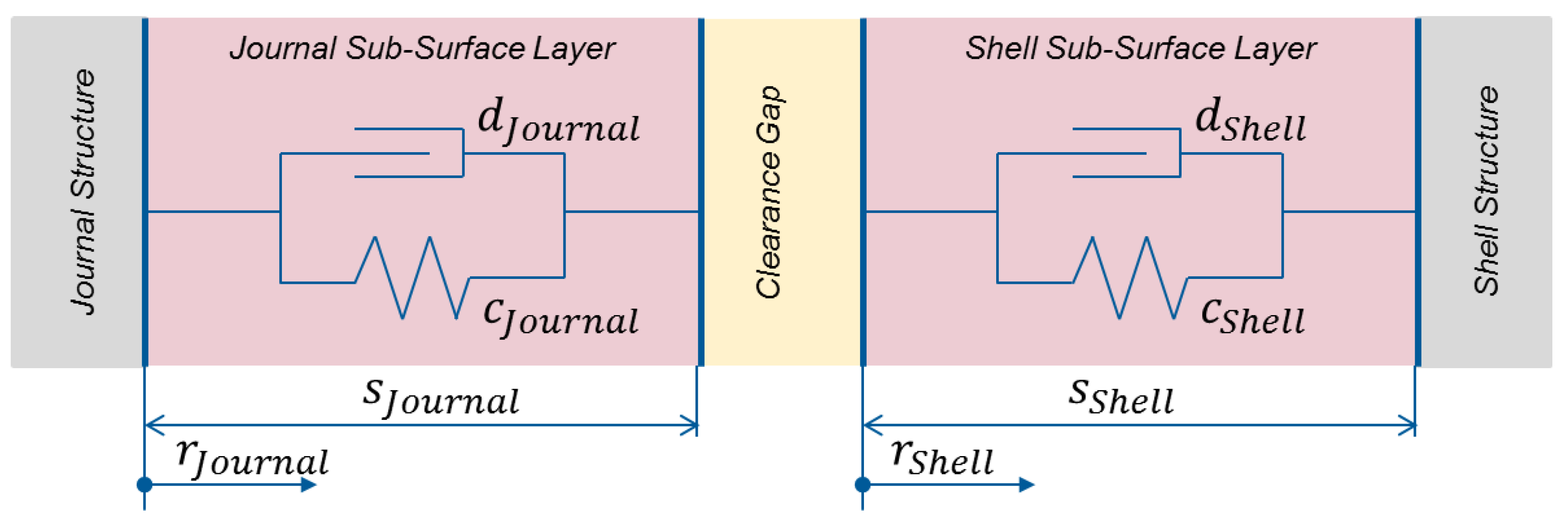
3.3. Surface Layer
In
Section 2, the interaction of structured or FEM models, which represent bodies, and joints is outlined. In the case of a joint being represented by an averaged Reynolds equation, the equation is solved on a finite volume grid. In typical applications, the discretization of the finite volume grid is several times finer compared to a usual body surface discretization using structured or FEM models. An alternative usage of a finer body discretization, which considers the detailed composite structure of the bearing shell, would increase the overall required computation times drastically and is therefore no option. However, in order to consider local deformation phenomena, as they happen, for instance, in the case of coatings with low Young’s modulus, appropriately, a fine spatial discretization of each body surface is also required. For this purpose, a surface layer is introduced in this section. Beside the numerical advantages, the surface layer approach offers the possibility to modify the surface layer properties for parameter variations without the need to update the FEM model.
Figure 6.
Surface contact layer on the journal and shell side.
Figure 6.
Surface contact layer on the journal and shell side.
The interpolation of clearance gap data and is done in several steps. Positions and velocities of connected component surface nodes in direction perpendicular to the surface are interpolated considering both gross motions as, for instance, position and angular position of a connecting rod, and local deformations as, for instance, deformation due to combustion load. Initially, the surface nodes are positioned at a nominal shape, which is a cylinder shape in the case of a big end bearing. Besides this, deviations from the nominal contours at different magnitude levels need to be considered. Both deviations at a large magnitude level, as, for instance, wedge contours, and deviations at a microscopic roughness level need to be considered. The large deviations are supposed to be static and are superimposed as profiles. The microscopic roughness level is represented by flow factors in the incorporated equations.
For both surfaces of contact, a surface layer based on the finite volume grid is introduced to consider dynamic local deformations in perpendicular direction to the body surface (
Figure 6). The additionally considered deformation at an arbitrary time step
can be written as a sum
with
. In order to consider both elastic and plastic deformation, two contributions
and
are considered, respectively
The body-specific radial shell deformation
is integrated from the radial shell deformation of the previous time step
according to
considering a time step size
and a damping-stiffness ratio
is the radial surface layer damping and
is the stiffness of the radial surface layer stiffness
with the Young’s modulus
, the layer thickness
and the progression rate
. Note that in the case of a positive
a progressive stiffness is considered, whereas in the case of
the applied stiffness is linear.
For distinguishing between elastic and plastic deformation, an additional switch function
is introduced
, the total (hydrodynamic and asperity) pressure in the clearance gap, and is the contact surface hardness.
Using
the local pressure
can be written as
Thus, depending on
, an elastic or a plastic local surface deformation is integrated by equation (8).
4. Results
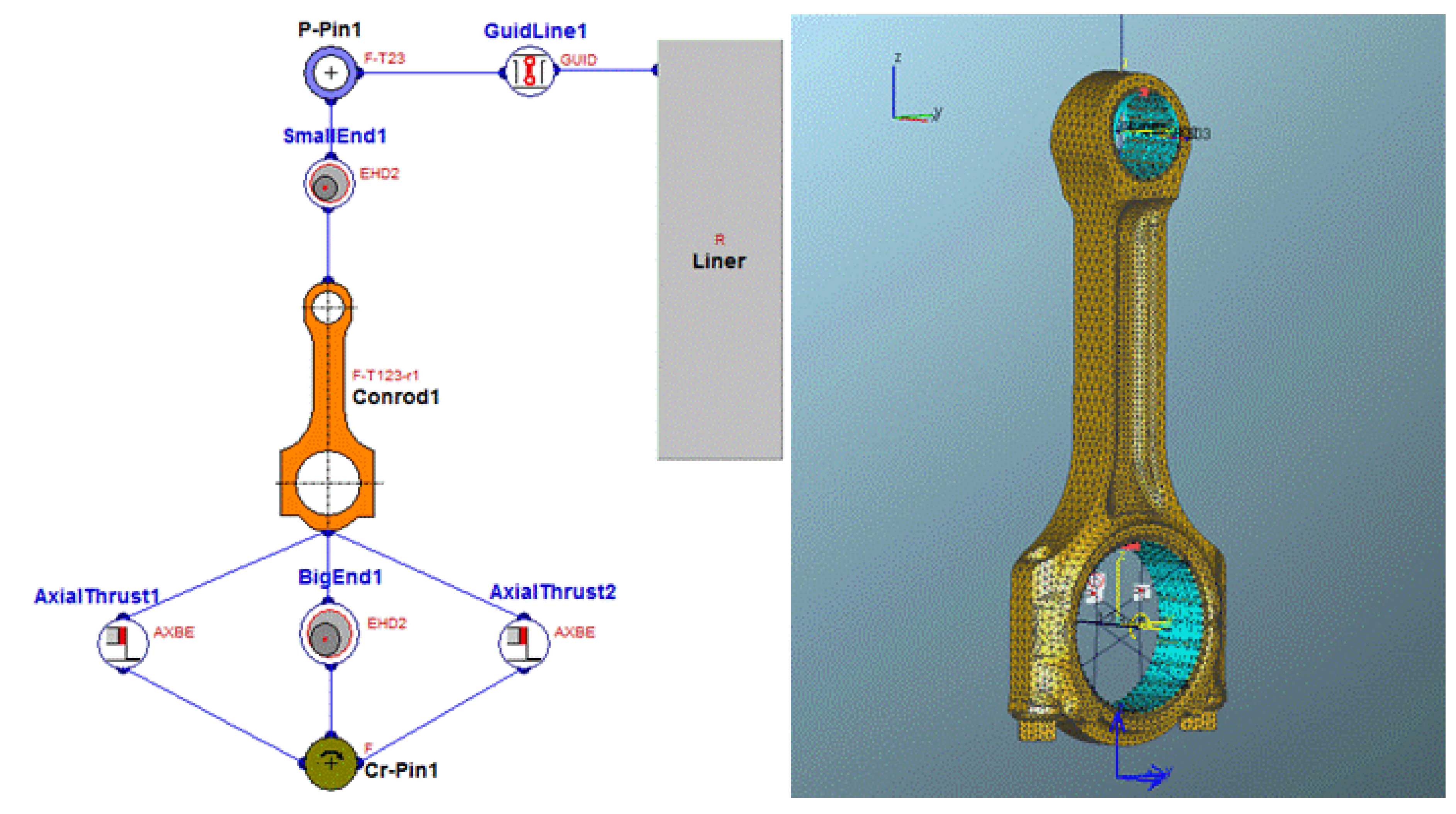
An influence study on friction loss power of different bearing shell types is presented in this section. The influences are demonstrated by assembling the bearing shells in a connecting rod big end of a four-cylinder Diesel engine. For matters of simplicity, only one of the four cylinders is represented in the model.
The model consists of four flexible bodies—a connecting rod and a piston pin, a cylinder liner to guide the motion of the piston pin and a crank pin. The crank pin performs a circular motion with constant angular velocity and represents the motion of the crankshaft. The mass of the piston is considered in the piston pin. Both the piston and the crank pin are represented by structured models according to [
13], respectively. The connecting rod is represented as a solid FEM model, [
14]. The model is condensed in a pre-processing step. The complete workflow of condensation and the resulting equations of motion are outlined in [
15].
The piston pin is guided to move along a cylinder liner using a simple nonlinear spring-damper function, see Offner
et al. [
16]. Similar functions are also applied to model two axial bearings, which restrict the axial motion of the connecting rod.
An averaged Reynolds equation considering mass conservation in combination with a Greenwood-Tripp asperity contact model is used to represent the big end and the small end bearing.
A topologic as well as a three-dimensional representation of the model is depicted in
Figure 7.
Figure 7.
Topologic (left) and three-dimensional (right) representation of the connecting rod example.
Figure 7.
Topologic (left) and three-dimensional (right) representation of the connecting rod example.
Combustion forces are integrated from pre-calculated cylinder pressures and are applied as time dependent boundary conditions on the piston pin.
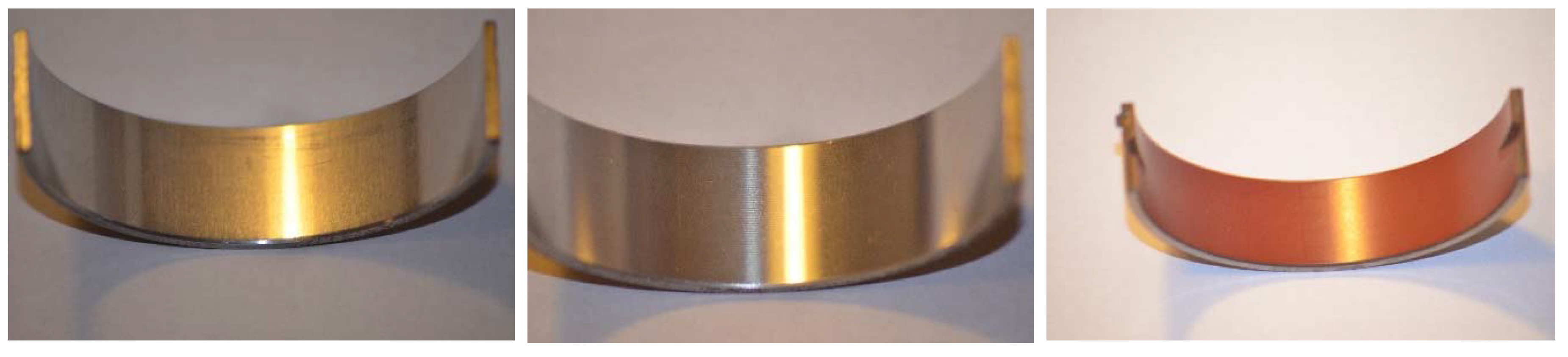
Figure 8.
Image of the AlSn-based plain (left) and grooved (middle) shell as well as of the polymer coated shell (right).
Figure 8.
Image of the AlSn-based plain (left) and grooved (middle) shell as well as of the polymer coated shell (right).
Figure 9.
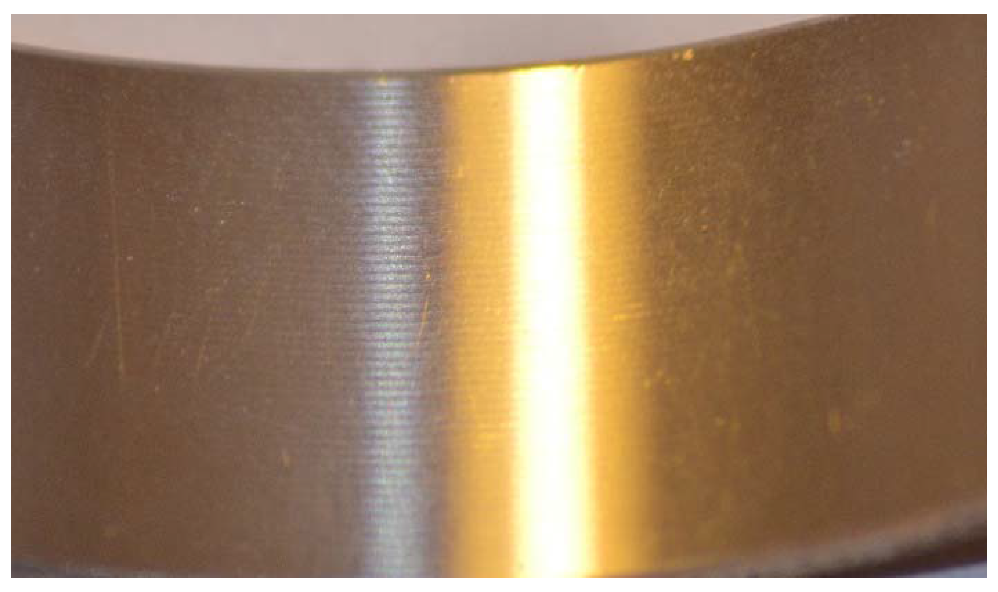
Image of the zoomed AlSn-based grooved shell surface.
Figure 9.
Image of the zoomed AlSn-based grooved shell surface.
Figure 10.
Measured deviation from nominal cylinder surface of the AlSn-plain shell.
Figure 10.
Measured deviation from nominal cylinder surface of the AlSn-plain shell.
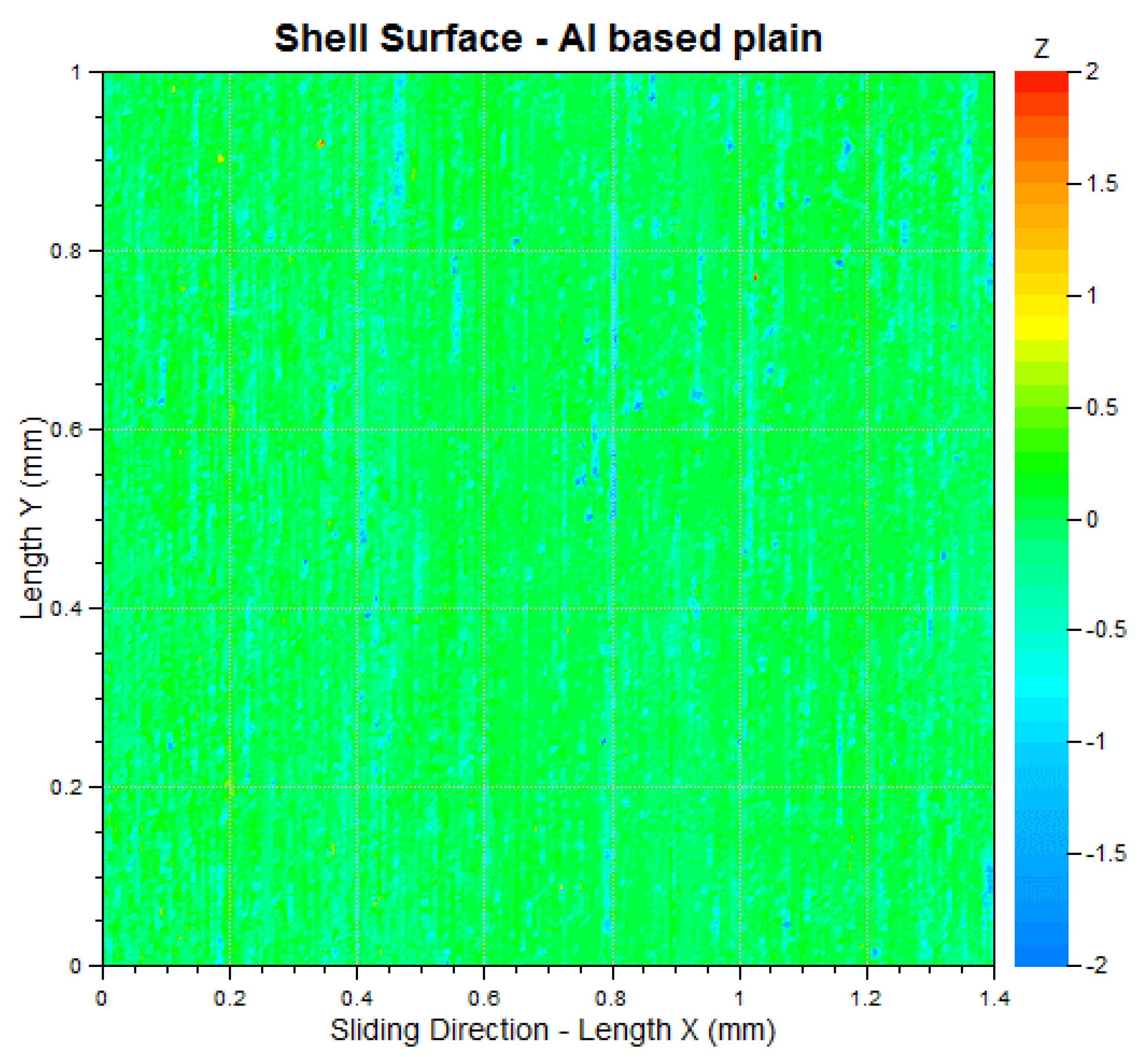
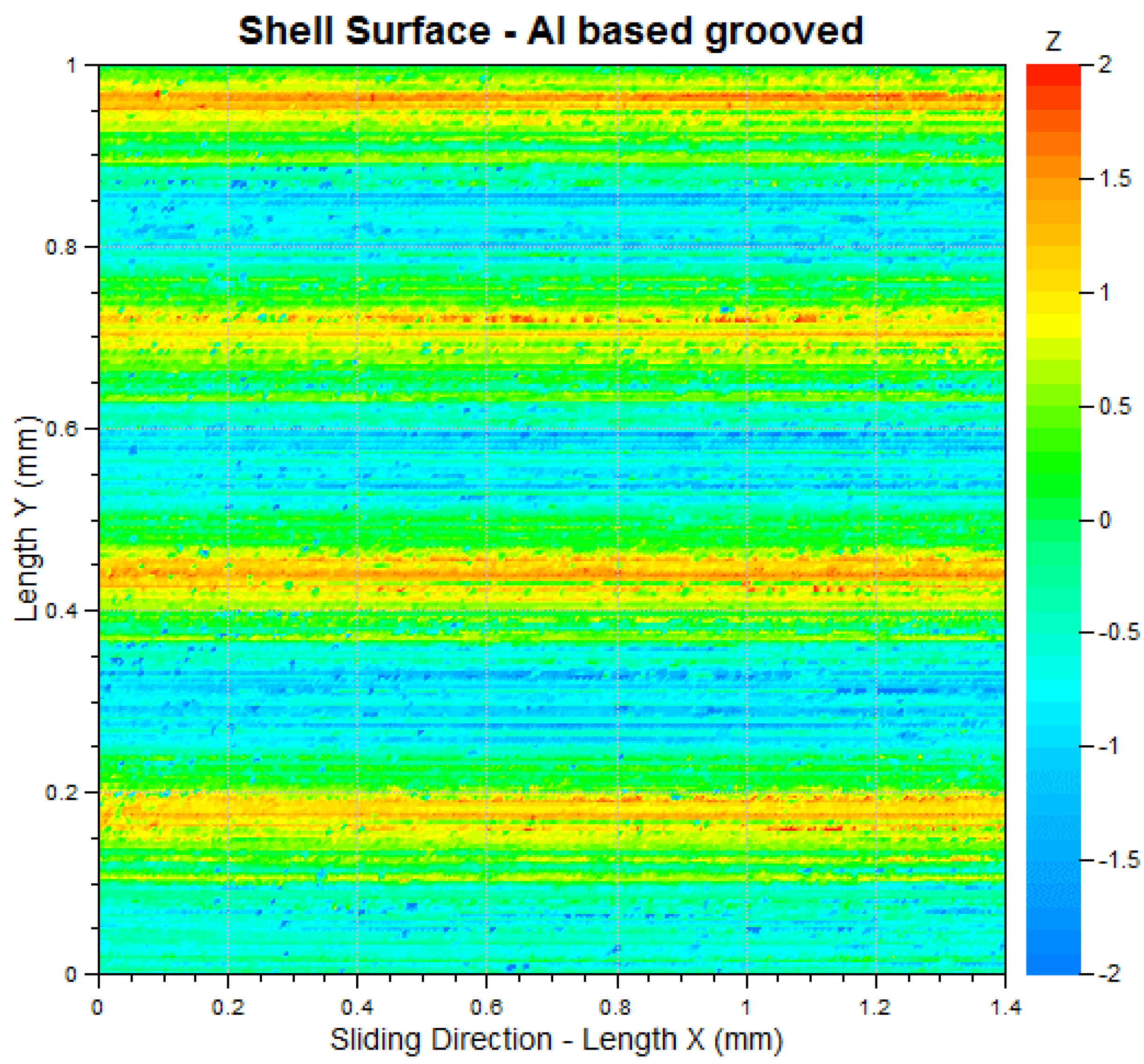
Three shells with different sliding layer types are used to instrument the big end bearing, a plain AlSn shell (
Figure 8, left), a grooved AlSn shell (
Figure 8, middle and
Figure 9) and a polymer coated (
Figure 8, right) shell.
Figure 10,
Figure 11 and
Figure 12 depict the measured deviation from a nominal cylinder surface of the three shell types, respectively. Comparing
Figure 10 and
Figure 11, the shape of the micro grooves in sliding direction can clearly be seen. Due to these micro grooves, the amplitude of deviation is also larger compared to the plain type. This deviation amplitude is also larger in case of the polymer coated shell (
Figure 12). This is caused by local deviations, which can clearly be seen in the figure.
Figure 11.
Measured deviation from nominal cylinder surface of the AlSn-grooved shell.
Figure 11.
Measured deviation from nominal cylinder surface of the AlSn-grooved shell.
Figure 12.
Measured deviation from nominal cylinder surface of the polymer coated shell.
Figure 12.
Measured deviation from nominal cylinder surface of the polymer coated shell.
From the measurements, derived shell and journal surface parameters are listed in
Table 1 and
Table 2. These are, in particular, the surface roughness and the roughness orientation to parameterize the Averaged Reynolds equation as well as the summit roughness and the mean summit height, which are required for the solid contact modelling.
Table 1.
Averaged Reynolds equation parameters for AlSn-plain, AlSn-grooved and polymer coated shell surface.
Table 1.
Averaged Reynolds equation parameters for AlSn-plain, AlSn-grooved and polymer coated shell surface.
| Surface | Surface roughness (µm) | Roughness orientation (-) |
|---|
| Shell | Journal | Shell | Journal |
|---|
| AlSn-plain | 0.300 | 0.242 | 0.539 | 10.298 |
| AlSn-grooved | 0.715 | 0.203 | 140.457 | 8.201 |
| Polymer coated | 0.547 | 0.214 | 1.006 | 9.393 |
Table 2.
Asperity contact parameters for AlSn-plain, AlSn-grooved and polymer coated shell surface.
Table 2.
Asperity contact parameters for AlSn-plain, AlSn-grooved and polymer coated shell surface.
| Surface | Summit roughness (µm) | Mean summit height (µm) |
|---|
| Shell | Journal | Shell | Journal |
|---|
| AlSn-plain | 0.220 | 0.173 | 0.250 | 0.203 |
| AlSn-grooved | 0.150 | 0.156 | 0.400 | 0.190 |
| Polymer coated | 0.402 | 0.163 | 0.546 | 0.185 |
For the polymer coated bearing, the surface layer module is also used to consider the elasto-plastic deformation off the coating layer. This is necessary because of the very low Young’s modulus of the polymer compared to white metal based bearing material. The used properties can be seen in
Table 3.
Table 3.
Surface contact layer specification.
Table 3.
Surface contact layer specification.
| | Shell |
|---|
| Layer thickness (mm) | 0.02 |
| Young’s modulus (N/mm²) | 2000 |
| Hardness (N/mm²) | 120 |
| Progression rate (-) | 1 |
| Damping stiffness ratio (s) | 1.0E-4 |
4.1. Exemplary Evaluation at a Predefined Operating Point
Equation (3) considers the friction coefficient as a sum of an abrasive, a solid (adhesive) and a hydrodynamic part.
Table 4 presents the friction coefficients for the three investigated bearing shell variants obtained at a predefined operating point. The assumptions for the operating point are an asperity contact pressure of
, a dynamic viscosity of
, a density of
, a conductivity of
, a specific heat capacity of
and a relative sliding velocity of
.
A comparison shows a significant difference between the aluminum shells and the polymer coated shell. The polymer coated shell has a significantly lower summed friction coefficient. This is mainly caused by the significantly lower adhesive friction part. On the other hand, the hydrodynamic friction coefficient dominates the adhesive friction coefficient in this case. In the two aluminum cases, adhesive friction dominates. Micro grooving the shell surface reduces the adhesive friction whereas the micro-hydrodynamic friction increases. The abrasive friction coefficient of the polymer coated shell is smaller compared to the one of the AlSn based shell. This is caused by the mainly elastic deformation of the polymer due to the asperity contact, whereas the AlSn material show mainly plastic deformation.
Table 4.
Adhesive, micro-hydrodynamic and summed friction coefficients for AlSn-plain, AlSn-grooved and polymer coated shell surface.
Table 4.
Adhesive, micro-hydrodynamic and summed friction coefficients for AlSn-plain, AlSn-grooved and polymer coated shell surface.
| Surface | Abrasive coefficient (-) | Adhesive coefficient (-) | Micro-hydrodynamic coefficient (-) | Summed coefficient (-) |
|---|
| AlSn-plain | 0.02 | 0.02 | 0.005 | 0.045 |
| AlSn-grooved | 0.02 | 0.015 | 0.007 | 0.042 |
| Polymer coated | 0.005 | 0.0025 | 0.01 | 0.0175 |
4.2. Dynamic Analysis Results
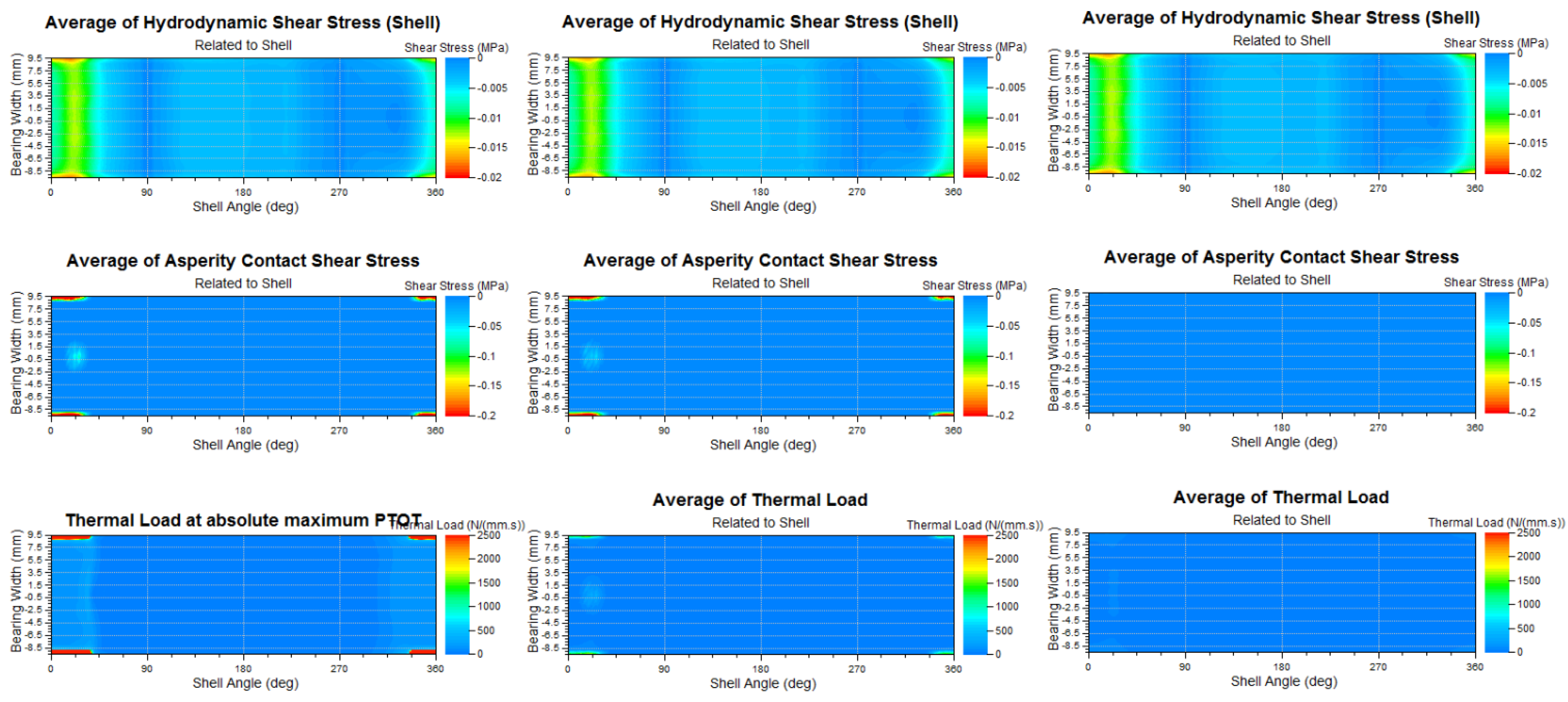
Figure 13 and
Figure 14 show results, which are obtained when using the three different bearing shell variants at an operating condition of 2000 rpm, full load, and within a dynamic analysis.
Two cycles are being calculated. As some initial conditions (local positions, orientations and velocities, oil fill ratio in clearance gap, oil temperature) are not known at the computation start, the corresponding quantities have to be presumed. These initial errors are reduced during the first cycle until reaching a cyclic steady state in the second cycle.
The average hydrodynamic and asperity shear stress as well as the thermal load distributions at absolute maximum peak total pressure are depicted.
The upper part of
Figure 13 shows a similar distribution of the averaged hydrodynamic shear stress, which acts on the shell surface. Maxima can be seen between 15- and 20-degree shell angles on both edges of the bearing shell.
The middle part of
Figure 13 compares the averaged asperity contact shear stress for the three variants. The two aluminum-based variants yield a similar distribution. The maximum values can again be found at both edges. In particular, maxima can be seen between 340 and 25-degree shell angles. Furthermore, a local maximum occurs in the center of the bearing shell approximately at a 20-degree shell angle. This is caused by the oil drilling outlet at the journal surface. The locally obtained asperity contact shear stresses are ten times larger compared to the equivalent hydrodynamics shear stresses. Different to the two AlSn variants, the polymer coated variant does not show the described phenomena. Thus, even if the polymer coated shell has larger deviations from the nominal cylinder surface (
Figure 12), it has lower friction due to lower asperity contact shear stress. This is due to increased micro-hydrodynamic effects and therefore reduced solid-to-solid contacts.
The lower part of
Figure 13 compares the thermal load distribution, obtained at the time point where the total absolute maximum peak pressure (hydrodynamic plus asperity) is reached. The plain AlSn variant shows significantly higher thermal loads at this point of time.
Figure 13.
Average hydrodynamic and asperity shear stress and thermal load at absolute maximum peak total pressure of AlSn-plain (left), AlSn-grooved (middle) and polymer coated (right) shell surface at 2000 rpm full load.
Figure 13.
Average hydrodynamic and asperity shear stress and thermal load at absolute maximum peak total pressure of AlSn-plain (left), AlSn-grooved (middle) and polymer coated (right) shell surface at 2000 rpm full load.
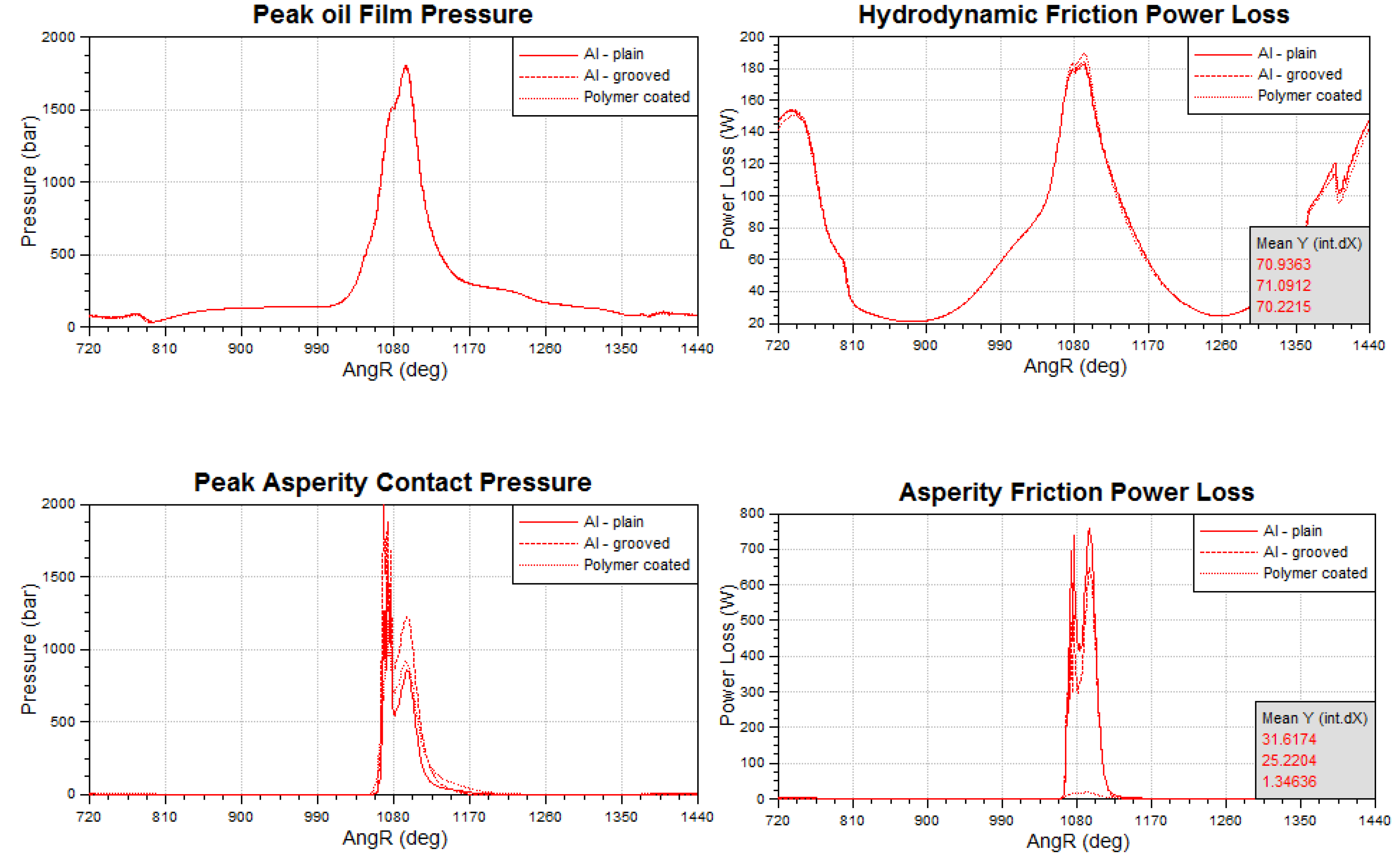
Figure 14.
Comparison of characteristic result quantities for three shell variants at 2000 rpm full load.
Figure 14.
Comparison of characteristic result quantities for three shell variants at 2000 rpm full load.
Figure 14 presents peak oil film and asperity contact pressure as well as hydrodynamic and asperity friction power loss over one engine cycle. Peak oil film pressure is almost equal, whereas the asperity contact pressure differs between the three variants. This difference also causes differences in obtained asperity friction loss power. The polymer coated variant yields only low asperity friction power loss compared to the other variants. Thus, the total friction power loss (
Table 5) of the polymer coated shell is significantly lower compared to the aluminum variants.
Table 5.
Total friction power loss for different surfaces.
Table 5.
Total friction power loss for different surfaces.
| Surface | Total Friction Power Loss (W) |
|---|
| AlSn-plain | 102.5 |
| AlSn-grooved | 96.2 |
| Polymer coated | 71.5 |


