An Adhesive Wear Model for Gears in Mixed Elastohydrodynamic Lubrication

Abstract

In this study, an adhesive wear model for a gear drive in mixed elastohydrodynamic lubrication (EHL) is proposed. The mixed-EHL model combines the average Reynolds equation with the ZMC rough-surface contact model to determine the asperity contact pressure. By incorporating the fractional film defect into the Archard wear equation, a wear rate model under mixed EHL is developed and verified against published experimental data. This wear-rate model is subsequently coupled with a transient line-contact mixed-EHL model for gears to establish a tooth-surface wear prediction model that iteratively updates the tooth geometry and contact pressure. The evolution of tooth-surface wear under mixed EHL is investigated, and the resulting wear characteristics are compared with those under dry-contact conditions. The influence of tooth-surface roughness is also systematically evaluated. The results indicate that tooth-surface wear is substantially reduced under mixed EHL and that the maximum wear occurs between the lowest point of single-tooth contact and the pitch point. Increasing surface roughness intensifies wear and shifts the maximum-wear location toward the tooth root. These findings demonstrate that appropriate lubricant selection and effective control of tooth-surface roughness are important for improving the wear resistance of gear drives.

1. Introduction

Gear drives generally operate under lubricated conditions. Proper lubrication allows a sufficiently thick oil film to form between the meshing tooth surfaces, preventing direct contact between the asperities on the surfaces and thereby avoiding wear [1]. However, manufacturing-induced roughness and the complex operating conditions of high-performance gear pairs can hinder the formation of a complete lubricant film. Under high loads, localized film breakdown may cause direct asperity contact, with the applied load shared by the lubricant film and the tooth-surface asperities. The resulting mixed-lubrication state produces tooth-surface wear, which can further degrade lubrication performance and accelerate other failure modes, including pitting and scuffing. Understanding tooth-surface wear under mixed lubrication is therefore important for improving the operational reliability of gear transmission systems.

Since Archard [2] introduced the adhesive-wear model in 1953, it has been widely applied to gear-wear prediction. Based on the Archard wear equation, Flodin and Andersson [3] developed a numerical model for mild wear in spur gears using a simplified inter-tooth load-distribution coefficient, a Winkler elastic-foundation model, and the single-point observation method to calculate contact pressure and sliding distance during meshing. They subsequently extended the approach to helical gears by using a slicing method [4,5]. Zhou and Wang [6] considered the actual meshing conditions of tooth-surface contact points and proposed a general sliding-distance model, which they combined with Hertzian contact theory and the Archard model to calculate adhesive wear in herringbone gears.

To overcome the accuracy limitations of analytical models, finite-element methods have been introduced to construct high-fidelity contact models and enable iterative wear calculations for complex gear geometries. Lundvall et al. [7] discretized the gear structure and, combining the Signorini contact formula, the Coulomb friction formula, and the Archard wear formula, used an improved Newton’s method to study wear in a heavy-duty truck transmission. Osman and Velex [8] used a finite-element-based load-distribution model to simulate mild abrasive wear in wide-faced solid spur and helical gears. Kahraman et al. [9] investigated the effect of tooth-profile deviations resulting from modification and manufacturing errors on helical gear wear, and Park and Kahraman [10,11] proposed a predictive model for hypoid gear wear and reduced the numerical cost through semi-analytical and surface-interpolation approaches. Huangfu et al. [12] constructed a multiphysics damage model coupling system elastic deformation with wear and pitting throughout the gear’s life. Although these approaches improve contact-pressure accuracy, they are computationally demanding and often neglect the lubrication state, motivating the transient line-contact mixed-EHL treatment developed here.

Regarding the wear under gear mixed lubrication, a great deal of research has been conducted in recent years. Akbarzadeh and Khonsari [13] combined wear models with the load-sharing concept to propose an accurate and efficient model for steady-state tooth-surface wear in spur gears under mixed lubrication. Masjedi and Khonsari [14] simultaneously solved the contact equations [15]—accounting for elastic, plastic, and elastoplastic deformation of surface micro-protrusions—and the mean-flow Reynolds equations [16], deriving the asperity load-carrying ratio; in combination with the mixed-lubrication wear model of Rowe [17], they further developed a rapid computational model for the wear rate of friction pairs [18] and applied it to steady-state spur-gear wear [19]. These studies established the load-sharing and fractional-film-defect concepts used in the present model; however, they are primarily based on steady-state or simplified gear representations and do not fully capture transient line-contact mixed-EHL behavior and iterative tooth-profile updating under heavy loads.

Experimental studies are essential for elucidating wear mechanisms and validating theoretical models. Krantz and Kahraman [20] and Sari and Haiahem [21] investigated the effects of lubricant viscosity, additives, and contamination on gear wear. Dizdar [22] studied the pitting resistance of sintered small-module gears, whereas Brandão et al. [23] determined average wear coefficients under various FZG operating conditions. Chin et al. [24] used absolute transmission error to assess tooth-surface wear, and Poletto et al. Lin [25] proposed a quantitatively distributed wear-measurement method for spur gears during micro-pitting and pitting tests. Other studies have combined simulations and experiments or developed dedicated twin-disc and in situ test methods to examine the effects of operating conditions and surface treatments [26,27,28,29]. In the present study, the twin-disc measurements of Wu and Cheng [30] are used to validate the wear-rate model.

Advances in sensing technology and artificial intelligence have also promoted vibration- and ultrasonic-based monitoring and life prediction for gear wear. Feng et al. [31,32] updated the wear coefficient in real time using measured vibration data and refined the model by considering Hertzian deformation and vibration cyclostationarity. Smith et al. [33] integrated gear-dynamics and tribological models to monitor and predict profile wear and pitting density. Wu et al. [34] developed an ultrasonic method for simultaneously monitoring lubricant-film thickness and coating wear, and Feng et al. [35] reviewed vibration-based gear-wear monitoring and prediction methods. Although condition monitoring is beyond the scope of this study, these investigations demonstrate the practical importance of reliable gear-wear prediction.

The published literature has substantially advanced gear-wear modeling and the theoretical and experimental analysis of EHL and mixed lubrication. Coupling between wear evolution and system dynamics, the influence of surface topography and operating parameters on lubrication regimes, and advanced condition-monitoring methods have also attracted considerable attention. Nevertheless, most existing wear-prediction methods are limited to dry contact or rely on simplified lubrication assumptions. A comprehensive adhesive-wear framework that simultaneously accounts for transient line-contact mixed EHL, asperity load sharing, fractional film defect, and iterative tooth-profile updating remains lacking for heavily loaded gear drives. The present study addresses this gap by integrating the average Reynolds equation with the ZMC rough-surface contact model and constructing a computational framework in which the worn tooth profile and the corresponding contact-pressure distribution are iteratively updated. The effects of lubricant selection and surface roughness are investigated to provide guidance for wear-resistant gear design.

2. Model

2.1. Mixed Elastohydrodynamic Lubrication Model in Line Contact

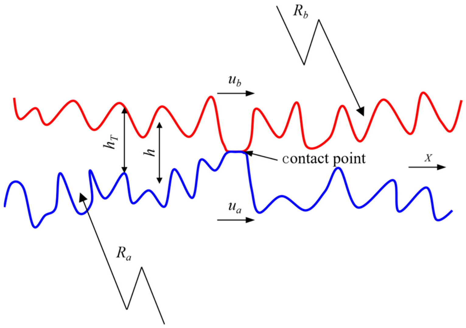
Two rough cylindrical surfaces with nominal radii R_a and R_b, respectively, are in contact under mixed lubrication, as shown in Figure 1, u_a and u_b represent the tangential velocities of cylinders a and b at the point of contact, h is the nominal oil film thickness, and h_T represents the actual oil film thickness.

2.1.1. Governing Equations

Based on the average Reynolds equation proposed by Patir and Cheng [16], the governing equations for the lubrication of a mixed elastohydrodynamic lubrication model in line contact can be written as

$${\displaystyle \frac{\partial }{\partial x}}\left({\varphi }_x{\displaystyle \frac{\rho h^3}{12\eta }}{\displaystyle \frac{\partial p_h}{\partial x}}\right)=u{\displaystyle \frac{\partial \left(\rho h_T\right)}{\partial x}}$$

(1)

In Equation (1), ρ is the density of the lubricant, η is the viscosity of the lubricant, and u is the rolling speed. ϕ_x is the pressure-flow coefficient in the x-direction, which can be expressed as

$$\left\{\begin{array}{l}{\varphi }_x=1-c{e}^{-r{\displaystyle \frac{h}{\sigma }}},\gamma \le 1\hfill \\ {\varphi }_x=1+c{\left({\displaystyle \frac{h}{\sigma }}\right)}^{-r},\gamma >1\hfill \end{array}\right.$$

(2)

here, c and r are both constants, and γ is the surface texture parameter (the aspect ratio of the asperities) defined as γ = λ_x/λ_y, where λ_x and λ_y are the autocorrelation lengths of the surface roughness in the x and y directions, determined from the surface autocorrelation function. We assume that the asperities follow a Gaussian distribution and that the roughness scales in the x and y directions are essentially the same, i.e., γ equals 1. Under these conditions, c is 0.9 and r is 0.56.

The oil film pressure must satisfy the boundary conditions: the oil film pressure at both the inlet and outlet boundaries is 0, while the oil film pressure in all other contact areas is greater than 0.

$$\left\{\begin{array}{l}{p}_h\left(x_i\right)=p_h\left(x_o\right)=0\hfill \\ p_h\left(x\right)\ge 0,x_i<x<x_o\hfill \end{array}\right.$$

(3)

where x_i and x_o represent the inlet and outlet boundaries, respectively.

Therefore, the equation for the nominal film thickness is

$$h=h_0+{\displaystyle \frac{x^2}{2R}}-{\displaystyle \frac{2}{\pi E^{\prime }}}{\displaystyle {\int }_{x_i}^{x_o}{p}_h}\ln \left(\left|x^{\prime }-x\right|\right)\mathrm{d}{x}^{\prime }$$

(4)

where h₀ is an unknown constant, and R and E’ are the equivalent radius of curvature and the modulus of elasticity, respectively.

The actual oil film thickness is

$$h_T=0.5h\left[1+\mathrm{erf}\left({\displaystyle \frac{h}{\sqrt{2}\sigma }}\right)+{\displaystyle \frac{\sigma }{\sqrt{2}\pi }}\exp \left({\displaystyle \frac{-h^2}{2{\sigma }^2}}\right)\right]$$

(5)

where, σ represents surface roughness, and the elliptic integral erf(y) can be expressed as

$$\mathrm{erf}\left(y\right)={\displaystyle \frac{2}{\sqrt{\pi }}}{\displaystyle {\int }_0^y{e}^{-{\delta }^2}\mathrm{d}\delta }$$

(6)

In Equation (1), both ρ and η depend on oil film pressure. The lubricant density is described by the Dowson–Higginson pressure–density relation [36], which is applicable within the pressure range considered in this study:

$$\rho ={\rho }_0\left(1+{\displaystyle \frac{0.6\times {10}^{-9}{p}_h}{1+1.7\times {10}^{-9}{p}_h}}\right)$$

(7)

where ρ₀ is the ambient density.

The pressure dependence of lubricant viscosity is described by the Roelands relation [37]:

$$\eta ={\eta }_0\exp \left\{\left(\ln {\eta }_0+9.67\right)\left[-1+{\left(1+5.1\times {10}^{-9}{p}_h\right)}^Z\right]\right\}$$

(8)

here, η₀ is the ambient viscosity, and Z is the viscosity-pressure index, which is expressed as

$$Z={\displaystyle \frac{\alpha }{5.1\times {10}^{-9}\left(\ln {\eta }_0+9.67\right)}}$$

(9)

According to the theory of load sharing under mixed lubrication, the load on the gears is shared by the oil film and surface asperities, so we have

$$w^{\prime }={\displaystyle {\int }_{x_i}^{x_o}{p}_h}dx+{\displaystyle {\int }_{x_i}^{x_o}{p}_a}dx$$

(10)

where p_a represents the contact pressure at the contact zone of the micro-protrusion.

2.1.2. Asperity Pressure

Since most surfaces in engineering applications conform to statistical laws, a statistical method is employed to determine the asperity pressure. The classic statistical method for rough surface modeling and contact analysis originates from the research of Greenwood and Williamson, who established a comprehensive theory of rough surface contact applicable to elastic contact. Through subsequent developments by other scholars, the CEB model—which accounts for elastic and plastic contact—and the ZMC model—which accounts for elastic, plastic, and elastoplastic contact—were gradually formulated [15]. The specific form of the ZMC model is as follows:

$$\begin{array}{ll}{p}_a& ={\displaystyle \frac{2}{3}}{E}^{\prime }n{\beta }^{0.5}{\sigma }^{1.5}\left({\displaystyle \frac{\sigma }{{\sigma }_s}}\right){\displaystyle \frac{1}{\sqrt{2\pi }}}{\displaystyle {\int }_{h^{\ast }-y_s^{\ast }}^{h^{\ast }-y_s^{\ast }+w_1^{\ast }}{w}^{\ast 1.5}{\varphi }^{\ast }\left(z^{\ast }\right)d{z}^{\ast }}\\ & +2\pi \cdot hd\cdot n\beta \sigma {\displaystyle \frac{1}{\sqrt{2\pi }}}\left({\displaystyle \frac{\sigma }{{\sigma }_s}}\right){\displaystyle {\int }_{h^{\ast }-y_s^{\ast }+w_2^{\ast }}^{\infty }{w}^{\ast }{\varphi }^{\ast }\left(z^{\ast }\right)d{z}^{\ast }}\\ & +\pi \cdot hd\cdot n\beta \sigma {\displaystyle \frac{1}{\sqrt{2\pi }}}\left({\displaystyle \frac{\sigma }{{\sigma }_s}}\right){\displaystyle {\int }_{h^{\ast }-y_s^{\ast }+w_1^{\ast }}^{h^{\ast }-y_s^{\ast }+w_2^{\ast }}{w}^{\ast }{\varphi }^{\ast }\left(z^{\ast }\right)\times \left[1-0.6\frac{\ln w_2^{\ast }-\ln w^{\ast }}{\ln w_2^{\ast }-\ln w_1^{\ast }}\right]}\\ & \times \left[1-2{\left({\displaystyle \frac{w^{\ast }-w_1^{\ast }}{w_2^{\ast }-w_1^{\ast }}}\right)}^3+3{\left({\displaystyle \frac{w^{\ast }-w_1^{\ast }}{w_2^{\ast }-w_1^{\ast }}}\right)}^2\right]d{z}^{\ast }\end{array}$$

(11)

where n is the density of the asperities, β is the radius of the asperity. h*, y*, s, w₁, w*, z*, w₂, and ϕ*(z*) are all dimensionless quantities, where h* = h/σ, y*s = y_s/σ, w*1 = w₁/σ, w* = w/σ, z* = z/σ, w*2= w₂/σ, ϕ*(z*) = ϕ(z)/σ, where w₁ is the normal strain at the initial yield threshold of the asperity, w is the normal strain of the asperity, w₂ is the normal strain at the threshold of complete plastic deformation of the asperity, and hd is the surface hardness of the softer material. The standard deviation σ_s of the rough surface height distribution relative to the average line of the surface peaks, the distance y_s between the average line of the rough surface and the average line of the surface peaks, and the probability density function ϕ(z) of the micro-peak height distribution can be expressed as:

$$\left\{\begin{array}{l}{y}_s={\displaystyle \frac{0.0459}{n\beta \sigma }}\hfill \\ {\sigma }_s=\sqrt{1-{\displaystyle \frac{3.7169\times {10}^{-4}}{{\left(n\beta \sigma \right)}^2}}\sigma }\hfill \\ \varphi \left(z\right)={\displaystyle \frac{1}{\sqrt{2\pi }\sigma }}\exp \left(-{\displaystyle \frac{z^2}{2{\sigma }^2}}\right)\hfill \end{array}\right.$$

(12)

2.1.3. Solution Method

To facilitate numerical calculations, these basic equations must be converted to a dimensionless form using the following dimensionless parameters: W = w′/(E′R), H = hR/(B²), $\overline{\rho }$ = ρ₀, $\overline{z}$ = zR/(B²), X = x/B, $\overline{y}s$ = ysR/(B²), $\overline{\eta }$ = η/η₀, P = p/pH, $\overline{\sigma }$ = σR/(B²), β = βR/(B²), V = hd/E′, U = uη₀/(E′R), $\overline{n}$ = n(B²/R)². The dimensionless form of the average Reynolds equation is

$${\displaystyle \frac{\partial }{\partial \mathrm{X}}}\left({\epsilon }_x{\displaystyle \frac{\partial P_h}{\partial X}}\right)={\displaystyle \frac{\partial }{\partial \mathrm{X}}}\left(\overline{\rho }{H}_T\right)$$

(13)

where

$$\left\{\begin{array}{c}{\epsilon }_x={\varphi }_x{\displaystyle \frac{\overline{\rho }{H}^3}{\overline{\eta }\lambda }}\\ \lambda ={\displaystyle \frac{3\mathrm{U}{\pi }^2}{4W}}\end{array}\right.$$

(14)

The dimensionless form of the nominal film thickness equation is

$$H=H_{00}+{\displaystyle \frac{X^2}{2}}-{\displaystyle \frac{1}{\pi }}{\displaystyle {\int }_{X_i}^{X_o}{P}_h}\ln \left(\left|{\overline{X}}^{\prime }-\overline{X}\right|\right)d{\overline{X}}^{\prime }$$

(15)

The dimensionless form of the actual film thickness is

$$H_T=0.5H\left[1+\mathrm{erf}\left({\displaystyle \frac{H}{\sqrt{2}\overline{\sigma }}}\right)+{\displaystyle \frac{\overline{\sigma }}{\sqrt{2}\pi }}\exp \left({\displaystyle \frac{-H^2}{2{\overline{\sigma }}^2}}\right)\right]$$

(16)

The dimensionless form of the viscosity equation is

$$\overline{\eta }=\exp \left\{\left(\ln {\eta }_0+9.67\right)\left[{\left(1+5.1\times {10}^{-9}{p}_H{P}_h\right)}^Z\right]\right\}$$

(17)

The dimensionless form of the density equation is

$$\overline{\rho }=1+{\displaystyle \frac{0.6\times {10}^{-9}{p}_H{P}_h}{1+1.7\times {10}^{-9}{p}_H{P}_h}}$$

(18)

The dimensionless form of the load equilibrium equation is

$${\displaystyle {\int }_{X_i}^{X_o}{P}_h}dX+{\displaystyle {\int }_{X_i}^{X_o}{P}_a}dX={\displaystyle \frac{\pi }{2}}$$

(19)

The dimensionless form of the asperity pressure is

$$\begin{array}{ll}\hfill P_a& ={\displaystyle \frac{2}{3}}\overline{n}{\overline{\beta }}^{0.5}{\overline{\sigma }}^{1.5}{W}^{-0.5}\left({\displaystyle \frac{\overline{\sigma }}{{\overline{\sigma }}_s}}\right){\displaystyle {\int }_{h^{\ast }-y_s^{\ast }}^{h^{\ast }-y_s^{\ast }+w_1^{\ast }}{w}^{\ast 1.5}{\varphi }^{\ast }\left(z^{\ast }\right)d{z}^{\ast }}\hfill \\ & +2\pi V\overline{n}\overline{\beta }\overline{\sigma }{W}^{-0.5}\left({\displaystyle \frac{\overline{\sigma }}{{\overline{\sigma }}_s}}\right){\displaystyle {\int }_{h^{\ast }-y_s^{\ast }+w_2^{\ast }}^{\infty }{w}^{\ast }{\varphi }^{\ast }\left(z^{\ast }\right)d{z}^{\ast }}\hfill \\ & +\pi V\overline{n}\overline{\beta }\overline{\sigma }{W}^{-0.5}\left({\displaystyle \frac{\overline{\sigma }}{{\overline{\sigma }}_s}}\right){\displaystyle {\int }_{h^{\ast }-y_s^{\ast }+w_1^{\ast }}^{h^{\ast }-y_s^{\ast }+w_2^{\ast }}{w}^{\ast }{\varphi }^{\ast }\left(z^{\ast }\right)\times \left[1-0.6\frac{\ln w_2^{\ast }-\ln w^{\ast }}{\ln w_2^{\ast }-\ln w_1^{\ast }}\right]}\hfill \\ & \times \left[1-2{\left({\displaystyle \frac{w^{\ast }-w_1^{\ast }}{w_2^{\ast }-w_1^{\ast }}}\right)}^3+3{\left({\displaystyle \frac{w^{\ast }-w_1^{\ast }}{w_2^{\ast }-w_1^{\ast }}}\right)}^2\right]d{z}^{\ast }\hfill \end{array}$$

(20)

After the dimensionless transformation, the basic equations must be discretized. The average Reynolds equation can be discretized as

$${\displaystyle \frac{1}{\Delta X^2}}\left[{\epsilon }_{xi-1/2}{P}_{hi-1}-\left({\epsilon }_{xi-1/2}+{\epsilon }_{xi+1/2}\right)P_{hi}+{\epsilon }_{xi+1/2}{P}_{hi+1}\right]={\displaystyle \frac{{\overline{\rho }}_i{H}_{Ti}-{\overline{\rho }}_{i-1}{H}_{Ti-1}}{\Delta X}}$$

(21)

where

$$\left\{\begin{array}{c}{\epsilon }_{xi-1/2}={\displaystyle \frac{1}{2}}\left({\epsilon }_{xi-1}+{\epsilon }_{xi}\right)\\ {\epsilon }_{xi+1/2}={\displaystyle \frac{1}{2}}\left({\epsilon }_{xi}+{\epsilon }_{xi+1}\right)\end{array}\right.$$

(22)

The discrete form of the nominal film thickness equation is

$$H_i=H_{00}+{\displaystyle \frac{X_i^2}{2}}-{\displaystyle \frac{1}{\pi }}{\displaystyle \sum _{j=0}^n{K}_{i,j}{P}_{hj}}$$

(23)

where

$$\begin{array}{ll}\hfill K_{i,j}=& \left(i-j+1/2\right)\Delta X\left[\ln \left(\left|i-j+1/2\right|\Delta X\right)-1\right]-\hfill \\ & \left(i-j-1/2\right)\Delta X\left[\ln \left(\left|i-j-1/2\right|\Delta X\right)-1\right]\hfill \end{array}$$

(24)

The discrete form of the actual film thickness equation is

$$H_{Ti}=0.5H_i\left[1+\mathrm{erf}\left({\displaystyle \frac{H_i}{\sqrt{2}\overline{\sigma }}}\right)+{\displaystyle \frac{\overline{\sigma }}{\sqrt{2}\pi }}\exp \left({\displaystyle \frac{-H_i^2}{2{\overline{\sigma }}^2}}\right)\right]$$

(25)

The discrete form of the load balance equation is

$$\Delta X{\displaystyle {\displaystyle \sum _{j=0}^{n-1}}\left(P_{hj}+P_{hj+1}\right)}+\Delta X{\displaystyle {\displaystyle \sum _{j=0}^{n-1}}\left(P_{aj}+P_{aj+1}\right)}={\displaystyle \frac{\pi }{2}}$$

(26)

The discrete form of the asperity contact pressure is

$$P_a=P_{a_1}+P_{a_2}+P_{a_3}$$

(27)

where

$$P_{a_1}={\displaystyle \frac{1}{3V}}\overline{n}{\overline{\beta }}^{-0.5}{\overline{\sigma }}^{0.5}{C}_{on}\Delta Z_1{\displaystyle \sum _{m_1=1}^{M_1}\left[\begin{array}{l}{\left(Z_{m_1}^{\ast }-J_1\right)}^{1.5}\exp \left(-0.5{\left(\frac{\overline{\sigma }}{{\overline{\sigma }}_s}{Z}_{m_1}^{\ast }\right)}^2\right)\\ +{\left(Z_{m_1-1}^{\ast }-J_1\right)}^{1.5}\exp \left(-0.5{\left(\frac{\overline{\sigma }}{{\overline{\sigma }}_s}{Z}_{m_1-1}^{\ast }\right)}^2\right)\end{array}\right]}$$

(28)

$$P_{a_2}=\Delta Z_3{C}_{on}{\displaystyle \sum _{m_3=1}^{M_3}\left[\begin{array}{l}\left(Z_{m_3}^{\ast }-J_1\right)\exp \left(-0.5{\left(\frac{\overline{\sigma }}{{\overline{\sigma }}_s}{Z}_{m_3}^{\ast }\right)}^2\right)\\ +\left(Z_{m_3-1}^{\ast }-J_1\right)\exp \left(-0.5{\left(\frac{\overline{\sigma }}{{\overline{\sigma }}_s}{Z}_{m_3-1}^{\ast }\right)}^2\right)\end{array}\right]}$$

(29)

$$P_{a_2}={\displaystyle \frac{1}{2}}\Delta Z_2{\displaystyle \sum _{m_2=1}^{M_2}\left\{\begin{array}{l}\left(Z_{m_2}^{\ast }-J_1\right)\times \exp \left(-0.5{\left(\frac{\overline{\sigma }}{{\overline{\sigma }}_s}{Z}_{m_2}^{\ast }\right)}^2\right)\times \left[1-0.6\frac{\ln w_2^{\ast }-\ln \left(Z_{m_2}^{\ast }-J_1\right)}{\ln w_2^{\ast }-\ln w_1^{\ast }}\right]\times \\ \left[1-2{\left(\frac{\left(Z_{m_2}^{\ast }-J_1\right)-w_1^{\ast }}{w_2^{\ast }-w_1^{\ast }}\right)}^3+3{\left(\frac{\left(Z_{m_2}^{\ast }-J_1\right)-w_1^{\ast }}{w_2^{\ast }-w_1^{\ast }}\right)}^2\right]+\left(Z_{m_2-1}^{\ast }-J_1\right)\times \\ \exp \left(-0.5{\left(\frac{\overline{\sigma }}{{\overline{\sigma }}_s}{Z}_{m_2-1}^{\ast }\right)}^2\right)\times \left[1-0.6\frac{\ln w_2^{\ast }-\ln \left(Z_{m_2-1}^{\ast }-J_1\right)}{\ln w_2^{\ast }-\ln w_1^{\ast }}\right]\times \\ \left[1-2{\left(\frac{\left(Z_{m_2-1}^{\ast }-J_1\right)-w_1^{\ast }}{w_2^{\ast }-w_1^{\ast }}\right)}^3+3{\left(\frac{\left(Z_{m_2-1}^{\ast }-J_1\right)-w_1^{\ast }}{w_2^{\ast }-w_1^{\ast }}\right)}^2\right]\end{array}\right\}}$$

(30)

$$C_{on}=\pi V\overline{n}\overline{\sigma }{W}^{-0.5}\left({\displaystyle \frac{\overline{\sigma }}{{\overline{\sigma }}_s}}\right)$$

(31)

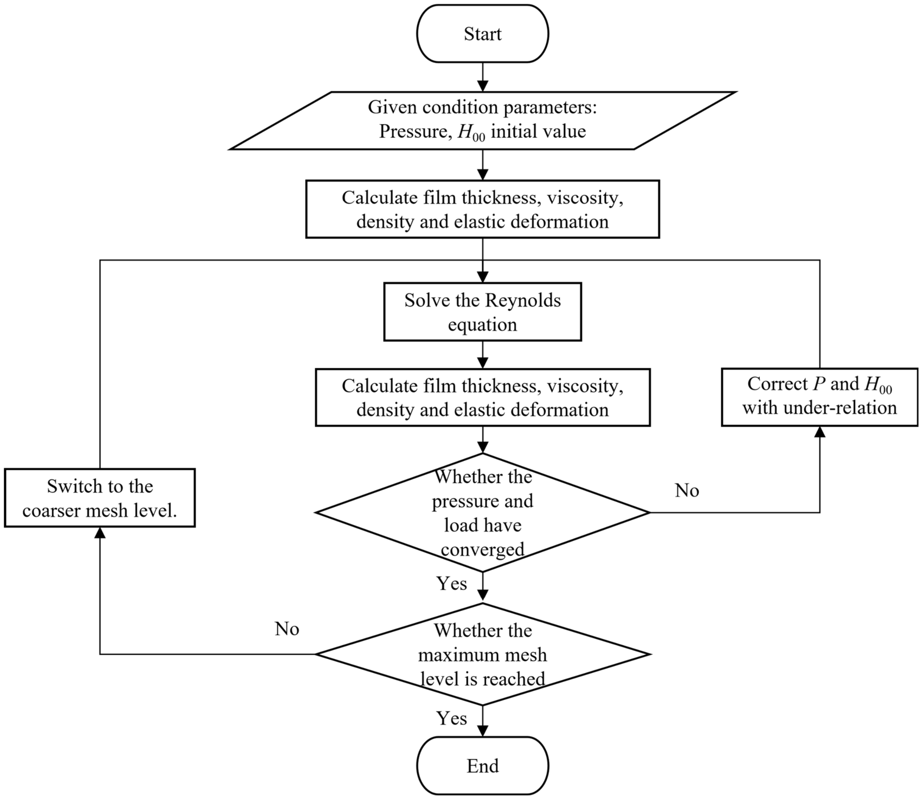
To improve computational accuracy and solution efficiency, the numerical solution method employs the Progressive Mesh Densification (PMD) method. This method first performs iterations on a sparse mesh; when the solution to the equation falls below a specified computational error threshold, it advances to the next level of a dense mesh to continue the iterations until the solution to the equation on the highest-level mesh simultaneously satisfies both the pressure convergence criterion and the load convergence criterion, as shown in Figure 2.

The results of the numerical calculations must satisfy the pressure convergence criteria and the load convergence criteria, that is,

$${\displaystyle \frac{\left|P-P_{OLD}\right|}{P}}\le E_{RP}$$

(32)

$${\displaystyle \frac{{\displaystyle {\int }_{X_i}^{X_o}\left|P-P_{old}\right|}dX}{{\displaystyle {\int }_{X_i}^{X_o}P}dX}}\le E_{RW}$$

(33)

The flowchart for the numerical solution is shown in Figure 3:

2.1.4. Validation of the Mixed EHL Model

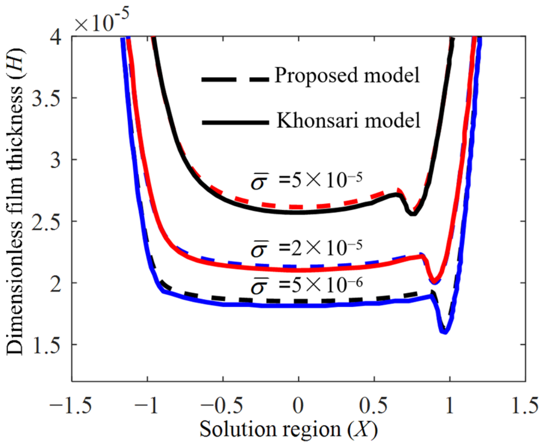
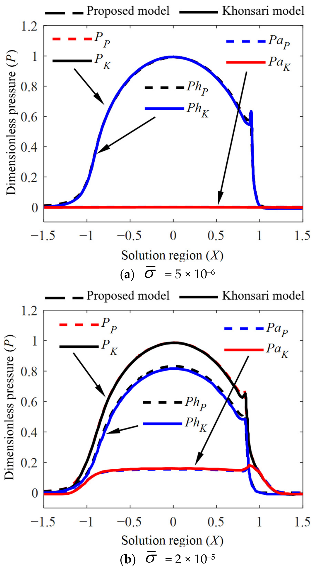
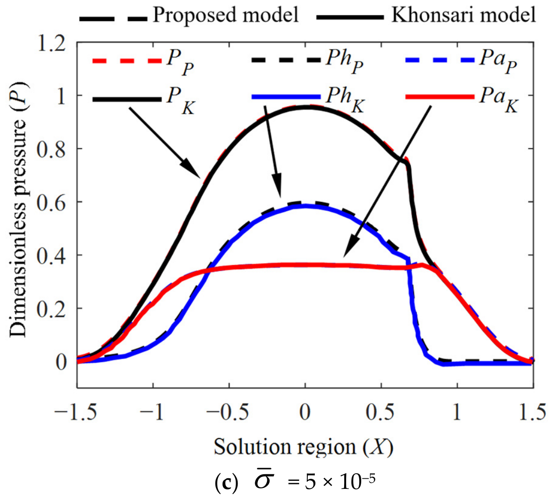
To verify the accuracy of the mixed lubrication model, a comparative analysis of the dimensionless oil film thickness and dimensionless contact pressure under different roughness conditions was conducted based on the parameters in Ref. [14]. The model in Ref. [14] simultaneously solves the Patir–Cheng average Reynolds equation, the elastic-deformation equation, and the ZMC asperity-contact model, with the total pressure shared by the lubricant film and asperities. The benchmark parameters are W = 1 × 10⁻⁴, U = 1 × 10⁻¹¹, G = 4500, and V = 0.01, while the dimensionless roughness values are $\overline{\sigma }$ = 5 × 10⁻⁶, 2 × 10⁻⁵, and 5 × 10⁻⁵. The asperity radius is selected such that $\overline{\sigma }/\overline{\beta }=0.01$.

The results are shown in Figure 4 and Figure 5, respectively. Figure 4 shows the distribution of the dimensionless oil film thickness for three surface roughness conditions. The solid lines represent the results from Ref. [14], while the dashed lines represent the results from the model presented in this work, with operating parameters of W = 1 × 10⁻⁴, U = 1 × 10⁻¹¹, G = 4500, V = 0.01. It is evident from the figure that, under different surface roughness conditions ($\overline{\sigma }$ = 5 × 10⁻⁶, 2 × 10⁻⁵, 5 × 10⁻⁵), the dimensionless oil film thickness distribution obtained by the presented model is essentially consistent with the published results; the distribution trends are consistent, and the numerical values are essentially equal. Specifically, the NRMSE values are 1.73%, 0.91%, and 1.02%, respectively, while the corresponding mean relative errors are 1.70%, 0.79%, and 0.95%. The maximum pointwise relative deviation among the three cases is 4.71%. These quantitative comparisons confirm that the present mixed-EHL model accurately reproduces the published numerical benchmark within the tested parameter range. As shown in Figure 4, the oil film thickness increases with increasing surface roughness. This is primarily attributed to the increased load borne by the asperities and their influence on the flow of the lubricating oil.

Figure 5 illustrates the specific distributions of oil film pressure, asperity pressure, and total pressure at different surface roughness levels corresponding to those in Figure 4, where P represents the total pressure, Ph represents the oil film pressure, and Pa represents the asperity pressure. The solid lines represent results from the references, distinguished by the subscript K; the dashed lines represent the results of the presented model, distinguished by the subscript P. As can be seen from Figure 5, for different surface roughness levels, the oil film pressure, asperity pressure, and total pressure calculated by the model in this work are consistent with the results in the references, further demonstrating the validity of the presented model. The data shown in Figure 5 indicate that as surface roughness increases, the oil film pressure gradually decreases, while the asperity pressure gradually increases. At the outlet, due to the contact of asperities, the total pressure is non-zero; as surface roughness increases, the position where the outlet pressure is zero moves farther away from the outlet. Furthermore, as surface roughness increases, the amplitude of the secondary pressure peak decreases, and the location of the pressure spike tends toward the center. For higher surface roughness values, the peak almost disappears. Due to contact between the asperities, the total pressure gradually extends in the direction of sliding as surface roughness increases, causing the maximum value of the total pressure to slowly decrease.

2.2. Wear Model of Mixed EHL in Line Contact

2.2.1. Wear Model

In a friction pair under mixed lubrication conditions, the load is shared by the lubricating oil film and asperities; wear occurs due to the contact between the asperities under relative sliding. By extending the adhesive wear rate model from dry contact conditions to mixed lubrication conditions, the following formula for the volumetric wear rate Ω_lub under mixed lubrication can be derived [18]

$${\Omega }_{\mathrm{lub}}=K\psi \left({\displaystyle \frac{L_a}{100}}\right){\displaystyle \frac{F{u}_s}{H}}$$

(34)

where K is the dimensionless wear coefficient; L_a is the percentage of load carried by surface asperities, representing the percentage of total pressure accounted for by the pressure from these asperities; F is the normal load; u_s is the relative sliding velocity; H is the surface hardness; and ψ is the fractional film defect, following the boundary-lubrication concept proposed by Kingsbury [38] and subsequently used in the lubricated adhesive-wear model of Rowe [17]. ψ represents the fraction or probability of asperity-contact sites that are not protected by adsorbed lubricant molecules and may equivalently be interpreted as the ratio of the unprotected metal-to-metal contact area to the real asperity contact area, which is expressed as follows:

$$\psi =1-\exp \left[-{\displaystyle \frac{D_a}{u_s{t}_0}}\exp \left(-{\displaystyle \frac{Q_a}{R_g{T}_s}}\right)\right]$$

(35)

In Equation (35), D_a is the molecular diameter of the oil film; t₀ is the fundamental time of molecular vibration in the adsorbed state; Q_a is the heat of the adsorbed film, which can be determined experimentally; R_g is the molar gas constant; and T_s is the contact temperature at the friction interface, which is composed of the body temperature T₀ and the flash temperature T_f, T_s = T₀ + T_f. L_a can be obtained from the model in Section 2.2; therefore, the only unknown quantity in Equation (35) is the contact temperature T_s.

The primary methods for calculating gear body temperature include the finite element method, the diffusion diagram method, and the thermal network analogy method. In this work, the thermal network method described in Ref. [39] is used to calculate the gear body temperature.

During the meshing process of gears, the rectangular contact area moves along the tooth height. According to the flash temperature formula proposed by Tian and Kennedy [40] for a rectangular heat source moving on a semi-infinite body:

$$T_f={\displaystyle \frac{qL}{\sqrt{\pi }(K_1\sqrt{1+P_{e1}}+K_2\sqrt{1+P_{e2}})}}$$

(36)

where q is the average heat flux generated by friction in the contact zone; L is the width of the contact zone; K₁ and K₂ are the thermal conductivities of the driving and driven gears, respectively; and P_e1 and P_e2 are the Peclet coefficients of the driving and driven gears, respectively. The expressions are as follows:

$$\begin{array}{l}{P}_{e1}={\displaystyle \frac{L\cdot u_1}{4k_1}},\\ P_{e2}={\displaystyle \frac{L\cdot u_2}{4k_2}}\end{array}$$

(37)

where u₁ and u₂ are the tangential velocities of the driving and driven gears, respectively, at the point of contact, and k₁ and k₂ are the thermal diffusivity coefficients of the driving and driven gears, respectively.

The formula for calculating the frictional heat flux q in Equation (36) is:

$$q=f_d\cdot u_s\cdot \overline{p}$$

(38)

where f_d is the coefficient of friction during dry meshing of the tooth surfaces, and $\overline{p}$ is the average contact pressure at the point of contact.

Under mixed lubrication conditions, the total heat flux q consists of the heat flux q_a from contact friction between the asperities and the heat flux q_h from shear friction in the lubricant, that is,

$$q=q_a+q_h$$

(39)

Based on Equation (38) and the theory of load sharing in mixed lubrication, the formula for calculating the contact friction heat flux q_a of a micro-protrusion is:

$$q_a=f_c\cdot u_s\cdot p_a=f_c\cdot u_s\cdot p(L_a/100)$$

(40)

where f_c is the coefficient of friction for a asperity body under unlubricated contact.

The shear friction heat flux q_h of the lubricating oil is calculated based on the limiting shear stress τ_lim of the lubricating oil [18], that is,

$$q_h={\tau }_{\lim }\cdot u_s$$

(41)

Based on the relationship between the limiting shear stress τ_lim of a lubricant and the oil film pressure, we have:

$${\tau }_{\lim }={\Lambda }_{\lim }\cdot p_h={\Lambda }_{\lim }\cdot p(1-L_a/100)$$

(42)

where Λ_lim is the limiting shear stress coefficient of the lubricant.

Solving the system of Equations (39)–(42), we obtain:

$$q=f_c\cdot u_s\cdot p(L_a/100)+u_s\cdot {\Lambda }_{\lim }\cdot p(1-L_a/100)$$

(43)

Substituting Equation (43) into Equation (36), the instantaneous temperature of the tooth surface of a spur gear pair at a given moment of meshing can be obtained. By combining this with the contact parameters during the meshing process, the distribution of the tooth surface wear rate from tooth engagement to disengagement can be determined.

2.2.2. Validation of the Wear Model

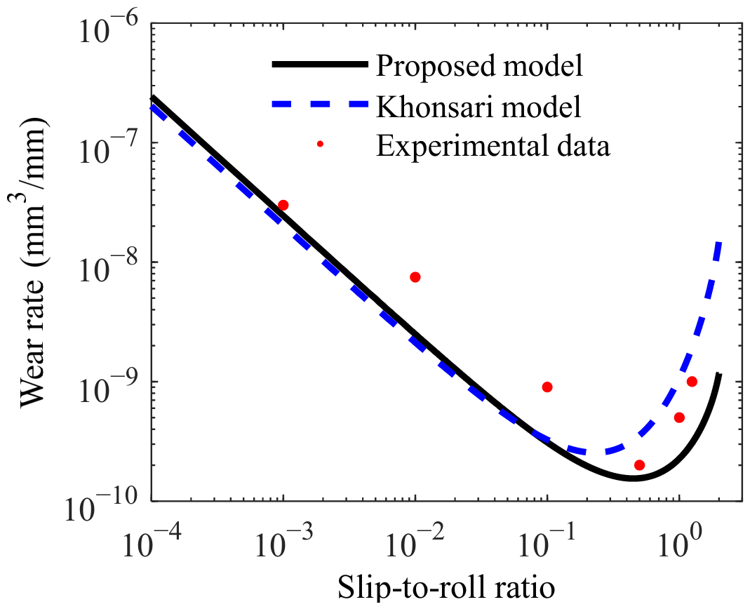
To simulate mixed lubrication under line contact conditions, Wu and Cheng [30] used a small dual-disk friction tester equipped with two independently driven motors, which allowed them to easily adjust the sliding-to-rolling ratio between the friction pairs. During the test, the rolling speed was kept constant (u_r = 1.83 m/s), and the sliding-to-rolling ratio was adjusted by varying the rotational speeds of the two disks. Lubricating oil is supplied on the inlet side of the contact point to ensure sufficient lubrication at the contact interface. The relevant parameters of the lubricating oil are: X = 3 × 10⁻¹⁰ m, t₀ = 3 × 10⁻¹² s, E_a = 49 × 10³ J/mol, and R_g = 8.31 J/(mol·K). Subsequently, Masjedi and Khonsari [18] conducted a theoretical study based on these experimental parameters, using a viscoelastic coefficient 5 × 10⁻⁸ m²/N, a limiting shear stress Λ = 0.06 MPa, and the following material parameters for the disks: thermal emissivity k₁ = k₂ = 1 × 10⁻⁵, thermal conductivity K₁ = K₂ = 60.5 W/(m·K), dimensionless dry wear coefficient K = 5 × 10⁻⁴, surface roughness σ = 0.34 μm, and asperity friction coefficient f_c = 0.12. Based on the above experimental parameters, the average Reynolds equation, and the formula for calculating the wear rate under mixed EHL, Figure 6 shows a comparison of the surface wear rates obtained using the model presented in this work with data from published studies.

As shown in Figure 6, the trends and numerical values of surface wear rates at different roll-to-slide ratios obtained from the proposed model show good agreement with both the experimental data from Wu and Cheng and the empirical formula from Masjedi and Khonsari. Compared with the results from Masjedi and Khonsari, the proposed model is closer to the experimental values, which demonstrates the validity of the proposed wear model.

2.3. Wear Model of Mixed EHL in Gears

2.3.1. Mixed EHL Model of Gear Drive

The lubrication problem for gear pair can be equivalently modeled as an infinitely long line-contact model. Due to the time-varying contact radius of the gear pair during meshing, transient effects must be taken into account; thus, the governing equation can be written as

$${\displaystyle \frac{\partial }{\partial x}}\left({\varphi }_x{\displaystyle \frac{\rho h^3}{12\mu }}{\displaystyle \frac{\partial p_h}{\partial x}}\right)=u{\displaystyle \frac{\partial \left(\rho h_T\right)}{\partial x}}+{\displaystyle \frac{\partial \left(\rho h_T\right)}{\partial t}}$$

(44)

For the relevant parameters in the equation, see Section 2.2.1.

The dimensionless form is

$${\displaystyle \frac{\partial }{\partial X}}\left({\epsilon }_x{\displaystyle \frac{\partial P_h}{\partial X}}\right)=C_u\left(t\right){\displaystyle \frac{\partial }{\partial \mathrm{X}}}\left(\overline{\rho }{H}_T\right)+{\displaystyle \frac{\partial }{\partial \overline{t}}}\left(\overline{\rho }{H}_T\right)$$

(45)

where C_u(t) = u(t)/u_e, where u(t) is the rolling speed during the meshing process, and u_e is the rolling speed at the node.

The discrete form is

$$\begin{array}{cc}\hfill {\displaystyle \frac{1}{\Delta X^2}}\left[{\epsilon }_{xi-1/2}{P}_{hi-1}-\left({\epsilon }_{xi-1/2}+{\epsilon }_{xi+1/2}\right)P_{hi}+{\epsilon }_{xi+1/2}{P}_{hi+1}\right]=C_u\left(\overline{t}\right)& {\displaystyle \frac{{\overline{\rho }}_i{H}_{Ti}-{\overline{\rho }}_{i-1}{H}_{Ti-1}}{\Delta X}}\hfill \\ & +{\displaystyle \frac{{\overline{\rho }}_i{H}_{Ti}-{\overline{\rho }}_i^{^}{H}_{Ti}^{^}}{\Delta \overline{t}}}\hfill \end{array}$$

(46)

Accordingly, the nominal film thickness equation becomes

$$h=h_0+{\displaystyle \frac{x^2}{2R\left(t\right)}}-{\displaystyle \frac{2}{\pi E^{\prime }}}{\displaystyle {\int }_{x_i}^{x_o}{p}_h}\ln \left(\left|x^{\prime }-x\right|\right)d{x}^{\prime }$$

(47)

where R(t) represents the total radius of curvature during gear meshing.

The dimensionless form is

$$H=H_{00}+{\displaystyle \frac{X^2}{2C_R\left(t\right)}}-{\displaystyle \frac{1}{\pi }}{\displaystyle {\int }_{X_i}^{X_o}{P}_h}\ln \left(\left|{\overline{X}}^{\prime }-\overline{X}\right|\right)d{\overline{X}}^{\prime }$$

(48)

where C_R(t) = R(t)/R₀, where R₀ is the reference radius of curvature.

The discrete form is

$$H_i=H_{00}+{\displaystyle \frac{X_i^2}{2C_R\left(t\right)}}-{\displaystyle \frac{1}{\pi }}{\displaystyle \sum _{j=0}^n{K}_{i,j}{P}_{hj}}$$

(49)

The load-balancing equation becomes

$$w^{\prime }\left(t\right)={\displaystyle {\int }_{x_i}^{x_o}{p}_h}dx+{\displaystyle {\int }_{x_i}^{x_o}{p}_a}dx$$

(50)

The dimensionless form is

$${\displaystyle {\int }_{X_i}^{X_o}{P}_h}dX+{\displaystyle {\int }_{X_i}^{X_o}{P}_a}dX={\displaystyle \frac{\pi }{2}}{C}_w\left(t\right)$$

(51)

where C_w(t) = w(t)/w₀, where w(t) is the load during the meshing process and w₀ is the total load.

The discrete form is

$$\Delta X{\displaystyle {\displaystyle \sum _{j=0}^{n-1}}\left(P_{hj}+P_{hj+1}\right)}+\Delta X{\displaystyle {\displaystyle \sum _{j=0}^{n-1}}\left(P_{aj}+P_{aj+1}\right)}={\displaystyle \frac{\pi }{2}}{C}_w\left(\overline{t}\right)$$

(52)

Using the load calculation model for asperity on tooth surfaces described in Section 2.1.2, solve the problem using the numerical calculation method described in Section 2.1.3.

2.3.2. Wear Depth of Gears in Mixed EHL

In Equation (34), Ω_lub represents the volumetric wear rate under mixed EHL (m³/s). Dividing both sides of the equation by the contact area A, and considering that the linear wear rate is Ω_lub = A·Δh (where Δh is the wear depth per unit time, in m/s) and P_a = (FL_a/100)/A, we obtain:

$$\Delta h={\displaystyle \frac{K\psi }{H}}{P}_a{u}_s$$

(53)

By integrating both sides of Equation (53) with respect to time t, we obtain the following formula for calculating the wear depth under mixed lubrication:

$$h={\displaystyle {\int }_0^t\frac{K\psi }{H}{P}_a{u}_s\mathrm{d}t}={\displaystyle \frac{K\psi }{H}}{P}_{a}S$$

(54)

where S represents the sliding distance.

By converting the equation to an integral form, we obtain the following formula for calculating the wear depth at any point p on the surface of the friction pair:

$$h_p={\displaystyle {\int }_0^s\frac{K\psi }{H}{P}_a}\mathrm{d}S$$

(55)

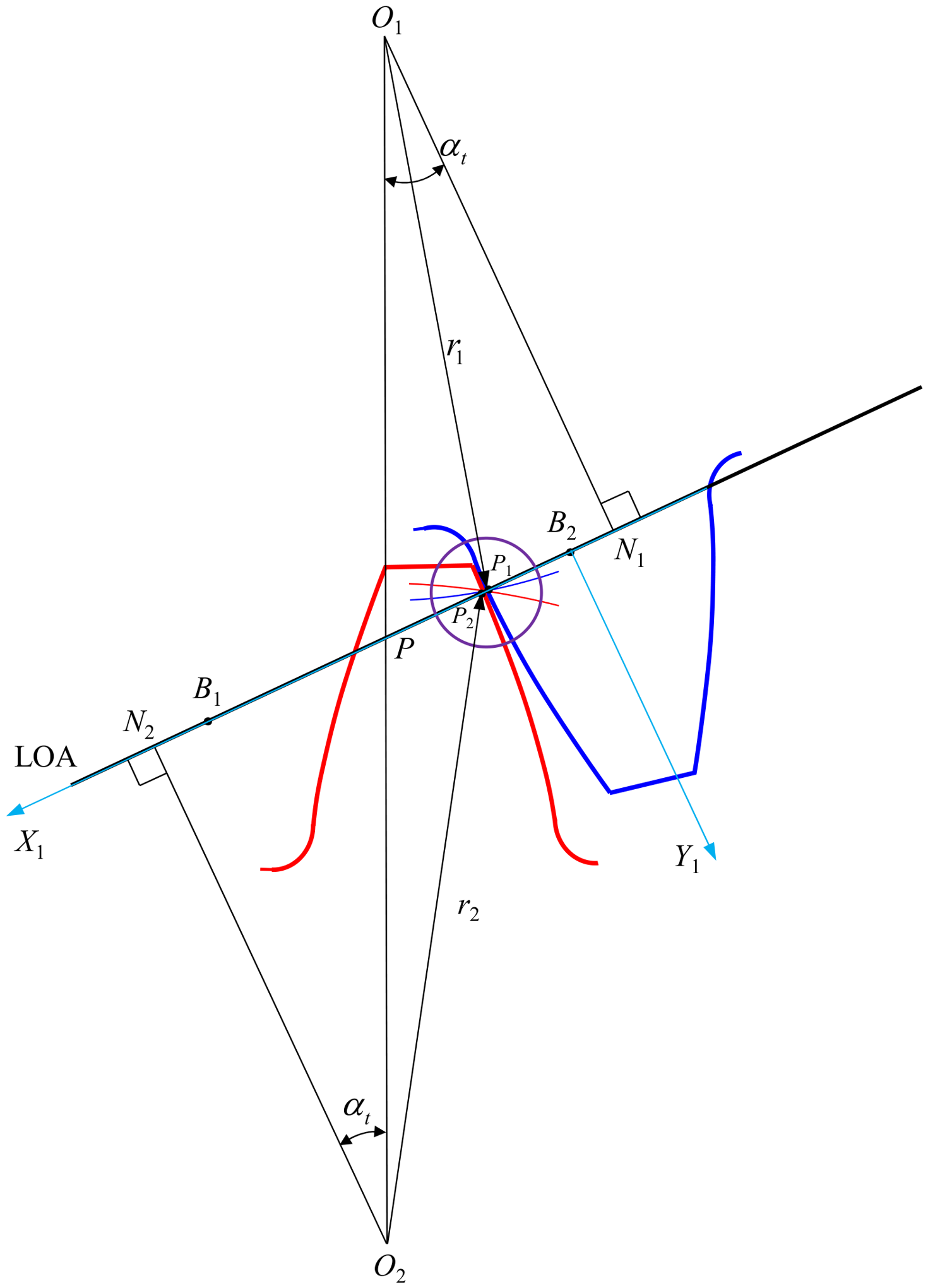
The engagement of the gear pair is shown in Figure 7, the blue and red curves represent the tooth profiles of the driving and driven gears, respectively. The gear pair enters engagement at B₂ and exits engagement at B₁. At any meshing instant, P₁ and P₂ are the corresponding contact points on the driving- and driven-gear tooth profiles and coincide at the instantaneous contact position. According to the involute gear-meshing principle, the successive contact positions lie on the straight line B₂B₁, which is the line of action. Therefore, each point on B₂B₁ represents a specific meshing instant, and progression from B₂ to B₁ represents the complete process from the start to the end of engagement. The ‘Direction of the line of contact’ used in the subsequent figures is thus defined as the direction from B₂ to B₁.

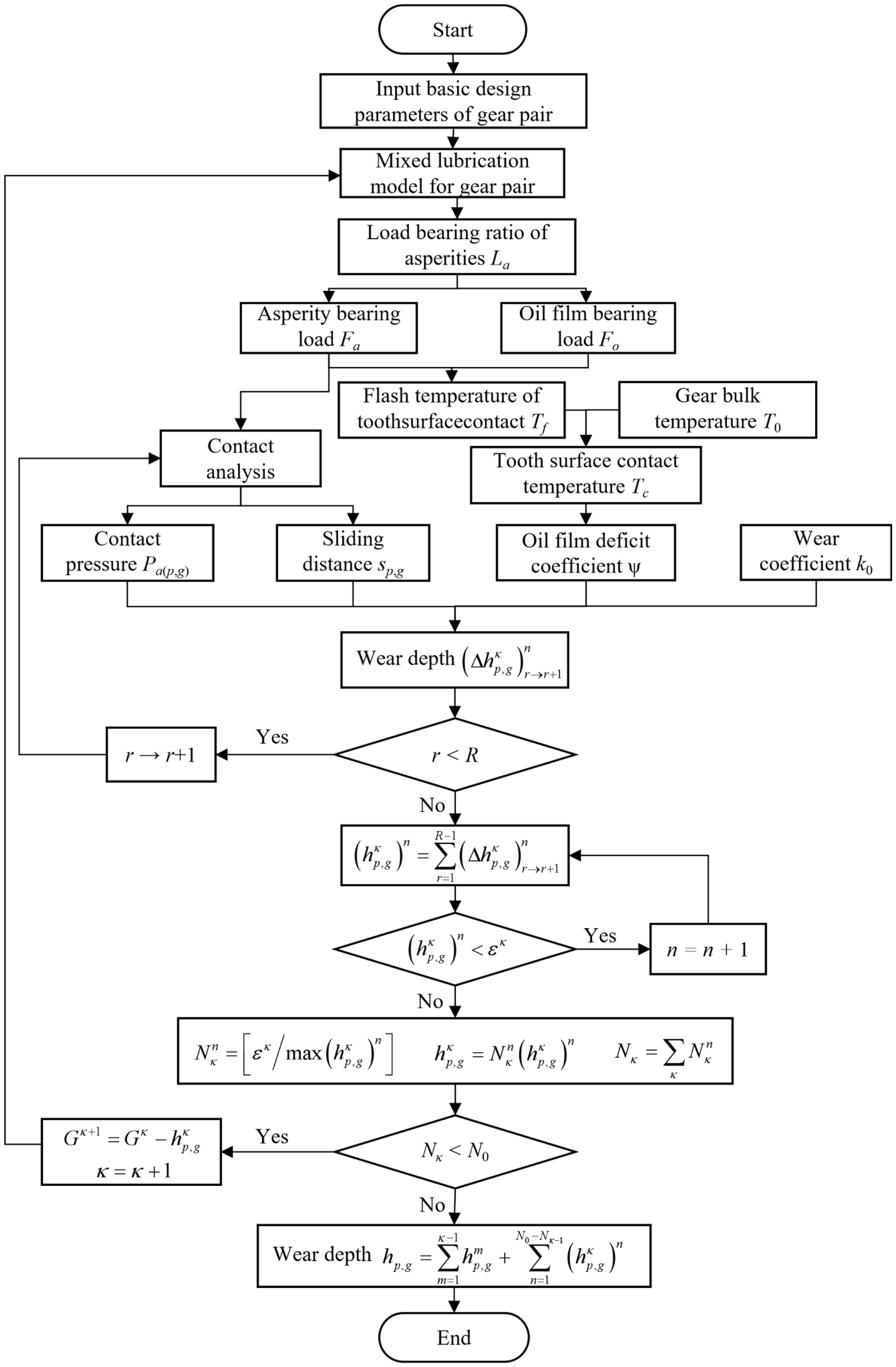
Based on the initial gear design parameters and the principle of generating gear surface cutting, the tooth surfaces of the driving gear and the driven gear are discretized into I and J nodes, respectively. The contact positions of the gear pair within one meshing cycle are discretized into R equal segments. The oil film deficiency coefficient ψ(r) and the asperity load ratio L_a(r) are calculated separately at position r (r = 1, 2, 3, …, R). Then, the contact pressure on the tooth surfaces of the driving and driven gears ${\left(P_i^{\kappa }\right)}_r^n$ (i = 1, 2, 3, …, I) and ${\left(P_j^{\kappa }\right)}_r^n$ (j = 1, 2, 3, …, J). Based on the sliding distances S_i,r→r+1 and S_j,r→r+1 at the discrete points on the driving and driven gears obtained using the single-point observation method, and in combination with the Archard wear equation, the formula for calculating the wear depth generated during the transition from contact position r to contact position r + 1 on the driving and driven gears is given by

$${\left(\Delta h_i^{\kappa }\right)}_{r\to r+1}^n={\displaystyle \frac{1}{2}}{k}_0\left[{\left(P_i^{\kappa }\right)}_r^n+{\left(P_i^{\kappa }\right)}_{r+1}^n\right]{\left(S_i^{\kappa }\right)}_{r\to r+1}^n$$

(56)

$${\left(\Delta h_j^{\kappa }\right)}_{r\to r+1}^n={\displaystyle \frac{1}{2}}{k}_0\left[{\left(P_j^{\kappa }\right)}_r^n+{\left(P_j^{\kappa }\right)}_{r+1}^n\right]{\left(S_j^{\kappa }\right)}_{r\to r+1}^n$$

(57)

where ${\left(\Delta h_i^{\kappa }\right)}_{r\to r+1}^n$ and ${\left(\Delta h_j^{\kappa }\right)}_{r\to r+1}^n$ represent the wear depths at discrete points on the tooth surfaces of the driving and driven gears, respectively.

During one meshing cycle, the cumulative wear depth on the tooth surface is

$${\left(h_i^{\kappa }\right)}^n={\displaystyle \sum _{r=1}^{R-1}{\left(\Delta h_i^{\kappa }\right)}_{r\to r+1}^n}$$

(58)

$${\left(h_j^{\kappa }\right)}^n={\displaystyle \sum _{r=1}^{R-1}{\left(\Delta h_j^{\kappa }\right)}_{r\to r+1}^n}$$

(59)

In a gear system operating under mixed EHL, tooth surface wear is minimal. Once wear accumulates to a certain extent, the gear system enters a phase of severe wear, the wear rate rises sharply, and the transmission system fails. Suppose that when the maximum wear depth at any discrete point on the tooth surface of the driving or driven gear reaches ε^κ, the tooth profile is updated; then, the number of meshing cycles for the gear pair at this point is

$$N_{\kappa }^n=\left[{\displaystyle \frac{{\epsilon }^{\kappa }}{\max \{{\left(h_i^{\kappa }\right)}^n,{\left(h_j^{\kappa }\right)}^n\}}}\right]$$

(60)

In Equation (60), [] denotes the floor function. At this point, the depth of tooth surface wear on the driving and driven gears is

$$h_i^{\kappa }={\displaystyle \sum _{n=1}^{N_{\kappa }^n}{\left(h_i^{\kappa }\right)}^n}$$

(61)

$$h_j^{\kappa }={\displaystyle \sum _{n=1}^{N_{\kappa }^n}{\left(h_j^{\kappa }\right)}^n}$$

(62)

After subtracting the wear depth from the tooth profile, calculate the updated tooth surface wear depth according to the procedure described above. The expression for the tooth surface wear depth after N₀ revolutions is

$$h_i={\displaystyle {\displaystyle \sum _{m=0}^{\kappa -1}}{h}_i^{\kappa }}+{\displaystyle {\displaystyle \sum _{n=1}^{N_0-N_{\kappa -1}^n}}{\left(h_i^{\kappa }\right)}^n}$$

(63)

$$h_j={\displaystyle {\displaystyle \sum _{m=0}^{\kappa -1}}{h}_j^{\kappa }}+{\displaystyle {\displaystyle \sum _{n=1}^{N_0-N_{\kappa -1}^n}}{\left(h_j^{\kappa }\right)}^n}$$

(64)

The calculation process for tooth surface wear under mixed EHL is shown in Figure 8.

3. Results and Discussion

3.1. Wear Evolution of Gears in Mixed EHL

For a gear pair operating under low-speed, heavy-load mixed lubrication conditions, the analysis is conducted based on the basic parameters of the gear pair in

Table 1. Parameters of the gear pair.

Parameters	Value	Parameters	Value
Number of teeth	Zp = 50, Zg = 50	Input speed	n1 = 80 r/min
Module	mn = 3 mm	Load torque	Tin = 800 N∙m
Pressure angle	α = 20°	Modulus of elasticity	E1 = 206 GPa, E2 = 206 GPa
Tooth width	B = 30 mm	Poisson’s ratio	μ1 = 0.3, μ2 = 0.3

. The relevant lubricant parameters are: α = 1.5 × 10⁻⁸ m²/N, Λ_lim = 0.065, and μ₀ = 0.08 Pa·s. It is assumed that when the surface roughness is 0.5 μm, the corresponding asperity friction coefficient is 0.135; when the surface roughness is 0.8 μm, the corresponding asperity friction coefficient is 0.15; and when the roughness is 1.2 μm, the corresponding asperity friction coefficient is 0.165. Taking the dimensionless wear coefficient K under dry contact conditions as 5 × 10⁻⁴ and the tooth surface hardness v as 6 GPa, the dimensional wear coefficient is 8.33 × 10⁻⁸ mm²/N.

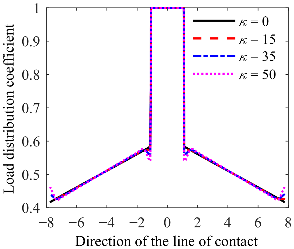
Tooth surface wear depth is relatively small under mixed EHL. To analyze the tooth surface wear behavior of a spur gear pair under mixed EHL more intuitively, the gear profile was updated after every 1 × 10⁶ meshing cycles. The load distribution coefficients for gear profile renewal frequencies of κ = 0, 15, 35, and 50 are shown in Figure 9. As can be seen from the figure, the load distribution coefficients under mixed EHL vary little, as the number of profile renewals increases, there is essentially no change at most meshing positions, except at the points of engagement, disengagement, and the alternating single-to-double tooth contact positions. This is primarily because the depth of tooth surface wear is relatively small under mixed EHL, and the change in tooth profile caused by wear has a minimal impact on meshing performance. Significant wear depth occurs at the alternating single- and double-tooth contact positions, causing the load distribution coefficient to decrease. Moreover, the more meshing cycles there are, the smaller the load distribution coefficient becomes. At the same time, the adjacent tooth pairs that are meshing are precisely at the moment of engagement or disengagement, so the load distribution coefficient of the adjacent tooth pairs increases as the number of meshing cycles increases.

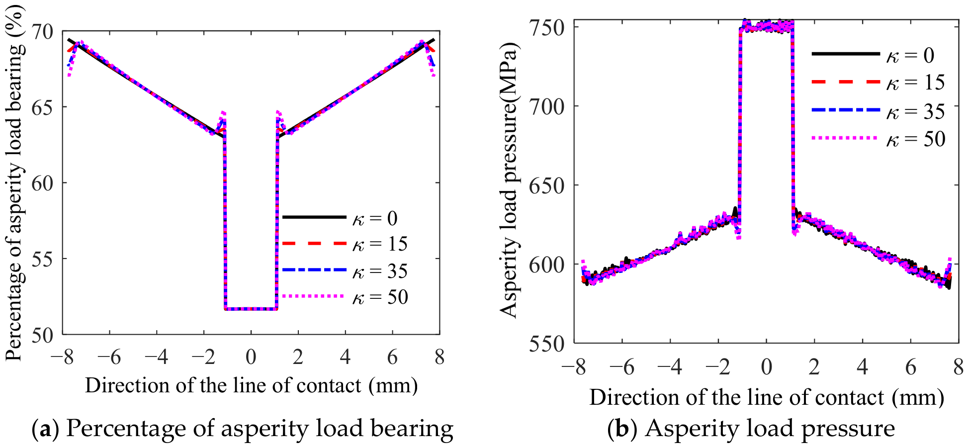
Figure 10 shows the percentage of load borne by asperities and the contact pressure for different numbers of tooth profile renewals. As shown in Figure 10a, the percentage of load borne by asperities on the tooth surfaces varies between 51.67% and 69.43% during a single meshing cycle. Compared to dry contact condition, part of the load between the meshing tooth surfaces is borne by the oil film, thereby preventing significant wear caused by direct metal-to-metal contact. The total load on a meshing gear pair in the double-teeth contact is smaller than in the single-tooth contact, yet the percentage of load borne by the protrusions is greater than in the single-tooth contact. This is primarily because, under high loads, the greater the deformation of the asperities, the easier it is for a good lubricating oil film to form on the meshing tooth surfaces, resulting in an increase in the proportion of load borne by the oil film and a decrease in the proportion borne by the asperities. However, because the total load increment in the single-tooth contact is large, even though the load-bearing percentage of the asperities in this zone is small, the total load borne by the asperities still increases, leading to higher load-bearing pressure on the asperities, as shown in Figure 10b. As the number of meshing cycles increases, the trend in the asperities’load-bearing percentage is opposite to that of the load distribution coefficient, whereas the trend in the load-bearing pressure of the asperities is consistent with that of the load distribution coefficient.

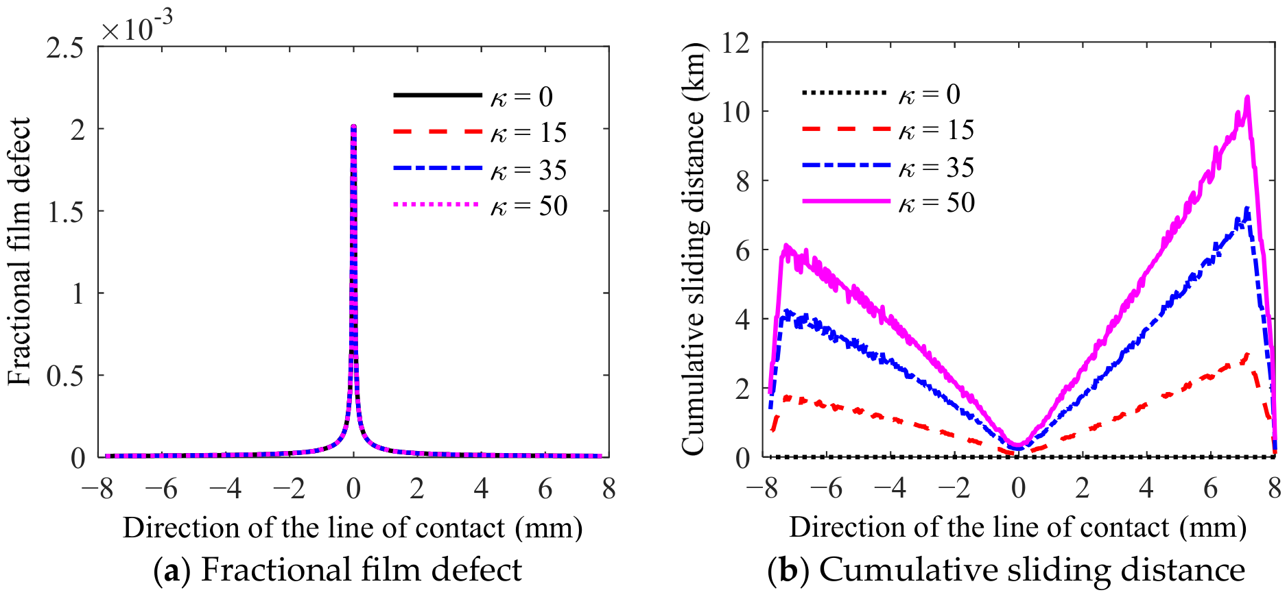
Figure 11 shows the variation in the oil film deficiency coefficient and the cumulative sliding distance during the meshing process. As can be seen from Figure 11a, from the engaging-in to the engaging-out, the oil film deficiency coefficient first increases and then decreases, reaching a maximum value of 2.01 × 10⁻³ at the pitch point and a minimum value of 8.85 × 10⁻⁶ at the engaging-in and engaging-out positions. Furthermore, the oil film deficiency coefficient is larger the closer the position is to the pitch point, primarily because this coefficient is related to the relative sliding velocity; at the pitch point, the relative sliding velocity is zero, resulting in the maximum value of the oil film deficiency coefficient. As shown in Figure 11b, the cumulative sliding distance on the tooth surface increases with the number of meshing cycles. Overall, it exhibits a distribution pattern that decreases sequentially from the tooth root to the pitch point and increases sequentially from the pitch point to the tooth tip.

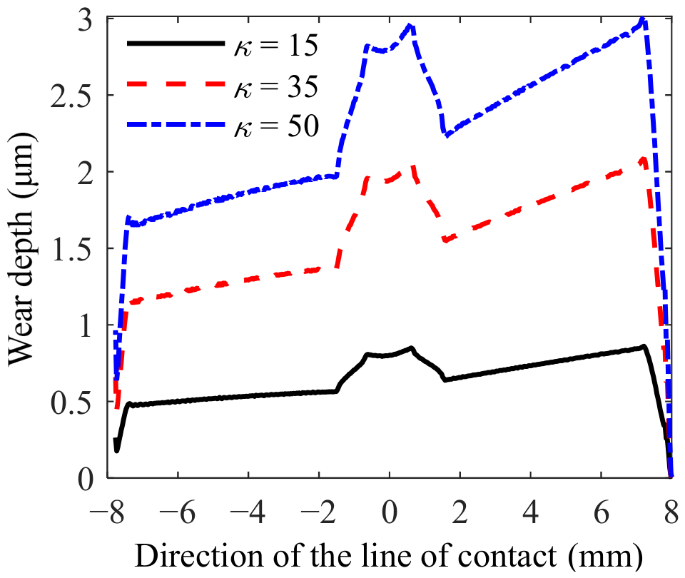
Based on the variation trends of asperity pressure, oil film depletion coefficient, and sliding distance, and in combination with the calculation model for tooth surface wear depth under mixed EHL, the tooth surface wear depth of the driving gear can be determined in Figure 12. For a meshing gear pair under mixed lubrication conditions, the tooth surface wear depth is relatively small. The wear depth in the single-tooth contact is relatively large, while in the double-teeth contact, the wear depth shows a gradual decrease from the point of engagement to the point of recession. The maximum tooth surface wear depth occurs between the lowest point of single-tooth contact and the pitch point, the wear depth at the pitch point position is not zero, a phenomenon that has been confirmed in numerous previous studies. When the number of tooth profile renewals, κ, is 15, 35, and 50, respectively, the maximum tooth surface wear depth is calculated to be 0.846 μm, 2.054 μm, and 2.96 μm, respectively; the wear depth at the root was calculated to be 0.840 μm, 2.046 μm, and 2.959 μm, respectively; the wear depth at the tip was calculated to be 0.477 μm, 1.166 μm, and 1.691 μm, respectively. From this, it can be inferred that as the number of gear meshing cycles increases, the rates of wear depth increase at the lowest point of a single tooth contact, the root, and the tip are essentially the same. This is primarily because the wear rate on the gear surfaces is low when the gear pair operates under mixed lubrication; the amount of wear generated on the gear surfaces is small, and its impact on the meshing condition is minimal, resulting in a largely linear increase in wear depth. It can be seen that if a gear transmission system operates under these conditions for an extended period, its service life can be significantly extended.

3.2. Wear Depths of the Gears Between the Mixed EHL and the Dry Contact

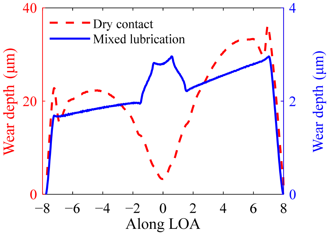
To conduct a comparative analysis of tooth surface wear characteristics under mixed lubrication and dry contact conditions, the tooth surface wear depths of the driving gear under these two operating conditions were compared. The results are shown in Figure 13. Since the wear coefficient, contact pressure, and sliding distance are higher under dry contact conditions, resulting in more pronounced wear, the total number of meshing cycles under dry contact conditions was set to 5 × 10³, with the tooth profile updated after every 100 meshing cycles; while under mixed lubrication conditions, the total number of meshing cycles was set to 5 × 10⁷, with the tooth profile updated after every 1 × 10⁶ meshing cycles. As shown in Figure 13, the gear pair operating under mixed EHL exhibits a smaller tooth surface wear depth. At 5 × 10⁷ meshing cycles, during the process from engagement to disengagement, the tooth surface wear depth decreases sequentially across the gear surface, except in the single-tooth contact, where the wear depth is relatively large. The maximum tooth surface wear depth occurs between the lowest point of single-tooth contact and the pitch point, with a value of 2.96 μm. Compared to the tooth root and tooth tip, the wear depth at the pitch point is greater, with a value of 2.81 μm. For the gear pair with the same parameters under dry contact conditions, the depth of tooth surface wear exhibits a distribution trend of first decreasing and then increasing from the engagement to the disengagement process. The maximum depth of tooth surface wear occurs at the tooth root, with a value of 36.21 μm. Compared to the tooth root and tooth tip, the depth of wear at the pitch point is smaller, with a value of 3.32 μm.

Figure 13 also shows that the distribution of tooth surface wear depth under mixed EHL is several orders of magnitude smaller than that under dry contact. In other words, for the same type of heavy-duty gear transmission, the use of lubricant can significantly reduce tooth surface wear. The reasons why tooth surface wear depth is smaller under mixed EHL than under dry contact can be summarized as follows: First, under mixed lubrication conditions, an oil film deficiency coefficient is introduced (Figure 11a), with values ranging from approximately 8.85 × 10⁻⁶ to 2.01 × 10⁻³. At most locations, the coefficient is on the order of 10⁻⁵, while only near the pitch point does it reach 10⁻³, significantly reducing the depth of tooth surface wear. Second, under mixed EHL, wear occurs only in the areas where the asperities bear the load, and the proportion of the total load borne by the asperities is only 50% to 70%, as can be seen in Figure 10a. Third, as the load borne by the asperities decreases, the contact width also decreases, thereby reducing the cumulative sliding distance of the tooth surface contact pairs. Under the combined influence of these three main factors, the depth of tooth surface wear under mixed EHL is significantly reduced, and the distribution pattern of wear depth differs considerably from that under dry contact conditions. This demonstrates that lubricants can greatly reduce tooth surface wear, and the use of lubricants is key to the anti-wear design of tooth surfaces.

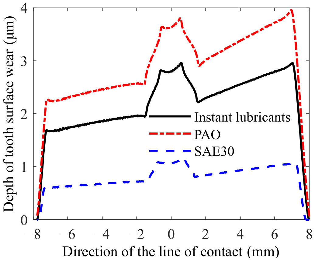
To investigate the effect of different lubricants on tooth surface wear in gear pairs under mixed EHL, two additional lubricants—poly-α-olefin (PAO) and engine oil (SAE30)—were selected for comparative analysis with the lubricant used in this study. The main parameters of PAO are: α = 1.5 × 10⁻⁸ m²/N, Λ_lim = 0.0434, μ₀ = 0.04 Pa·s; the main parameters of SAE30 are: α = 2.5 × 10⁻⁸ m²/N, Λ_lim = 0.091, μ₀ = 0.35 Pa·s. The distribution of tooth surface wear depth for the meshing gear pair at 5 × 10⁷ meshing cycles is shown in Figure 14. As shown in the figure, the trends in tooth surface wear depth distribution are generally consistent across the three lubricants, although there are differences in the specific values. For SAE30 lubricating oil, the tooth surface wear depths at the tooth root, the lowest point of single-tooth contact, and the tooth tip were calculated to be 1.077 μm, 1.153 μm, and 0.607 μm, respectively; for PAO lubricating oil, the tooth surface wear depths at the tooth root, the lowest point of single-tooth contact, and the tooth tip were calculated to be 3.958 μm, 3.808 μm, and 2.265 μm, respectively. Under constant operating conditions for the gear pair, different types of lubricants have a significant impact on tooth surface wear; the wear depth with PAO lubricant is approximately 3.4 times that of SAE30 lubricant. Therefore, for gear transmission systems operating under different conditions, selecting the appropriate type of lubricant can further improve the anti-wear performance of the gear teeth.

3.3. Effect of Surface Roughness on Tooth Surface Wear

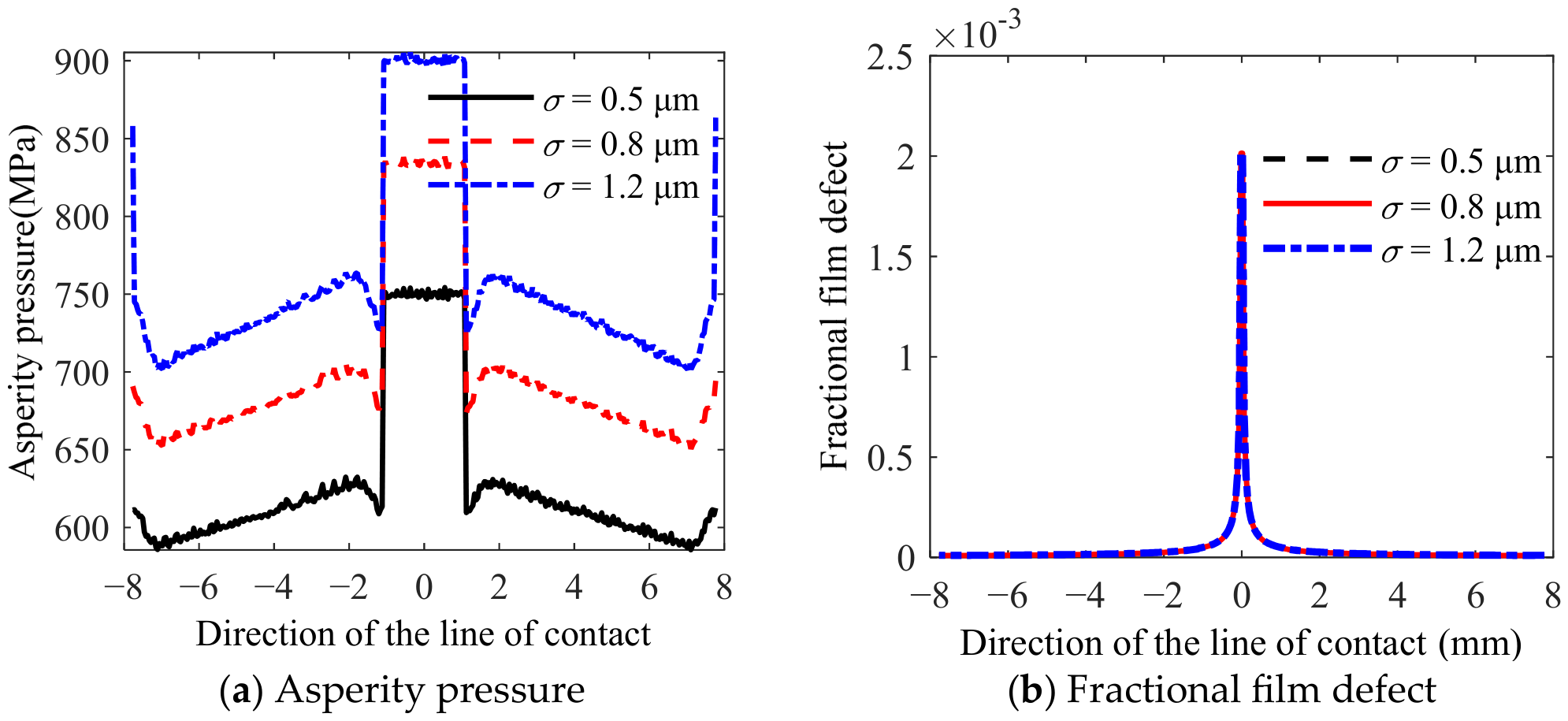
In the average Reynolds equation, because the pressure-flow coefficient ϕ_x, which is related to surface roughness, is introduced in Equation (2), it is of great significance to investigate the effect of surface roughness on the wear behavior of gear tooth surfaces under mixed EHL. The asperity pressure and fractional film defect for different roughness levels are shown in Figure 15. In Figure 15a, as surface roughness increases, the asperity pressure increases, as surface roughness σ increases from 0.5 μm to 1.2 μm, the maximum asperity pressure rises from 754.2 MPa to 904 MPa, an increase of 19.86%. This is primarily because the increase in surface roughness leads to a greater number of asperities in contact, thereby reducing the load-bearing capacity of the oil film. As tooth surface roughness increases, the pressure of the asperities at the engagement and disengagement positions rises more rapidly. However, surface roughness has a relatively minor effect on the fractional film defect, as shown in Figure 15b. This is primarily because the fractional film defect is related only to sliding speed and contact temperature; although tooth surface roughness affects contact temperature, its influence is negligible at low rotational speeds.

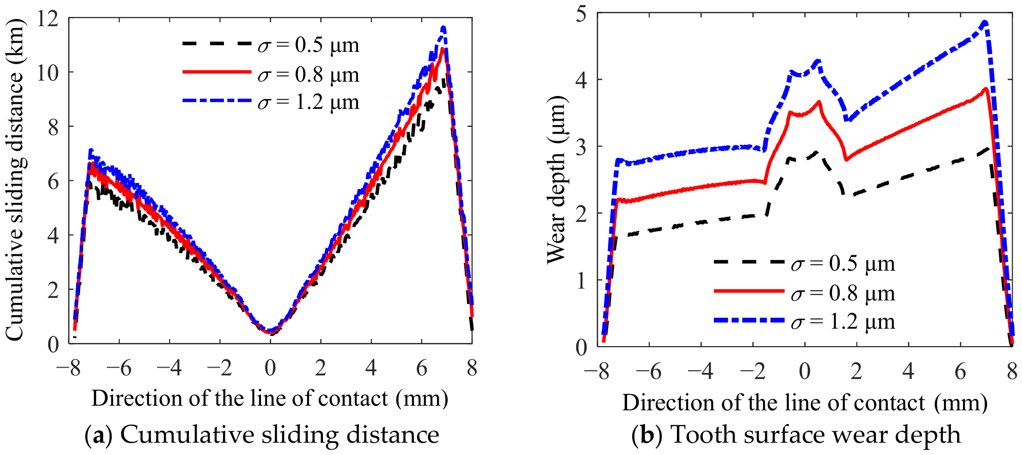
As surface roughness increases, the load-bearing pressure on the asperities increases, leading to an increase in contact width. Since the sliding distance is directly proportional to the contact width, the cumulative sliding distance also gradually increases (Figure 16a). Based on the variation patterns of the aforementioned parameters with respect to tooth surface roughness, the effects of different tooth surface roughness levels on the distribution of tooth surface wear depth under mixed EHL can be determined, as shown in Figure 16b. As tooth surface roughness increases, the depth of tooth surface wear also increases. The specific reason for this is that, apart from the oil film depletion coefficient being insensitive to changes in roughness, both the pressure exerted by the asperities and the cumulative sliding distance increase with increasing surface roughness. As the tooth surface roughness σ increased from 0.5 μm to 1.2 μm, the maximum wear depth at the tooth root increased from 2.959 μm to 4.862 μm, the maximum wear depth near the lowest point of single-tooth contact increased from 2.96 μm to 4.29 μm, and the maximum wear depth at the tooth tip increased from 1.691 μm to 2.805 μm—representing increases of 64.3%, 44.9%, and 65.9%, respectively. It can be concluded that as tooth surface roughness increases, the depth of tooth surface wear also increases, and the location of the maximum wear depth shifts from between the lowest point of single-tooth contact and the pitch point to near the tooth root. Therefore, minimizing tooth surface roughness as much as possible is also a critical aspect of tooth surface wear-resistant design.

3.4. Practical Implications for Gear Design and Manufacturing

The results obtained in this study provide several practical guidelines for the anti-wear design and manufacture of gear drives. First, the selection of the lubricant is of primary importance: for the operating conditions considered, the tooth-surface wear depth obtained with PAO is about 3.4 times that obtained with SAE30 (Figure 14), indicating that a lubricant with appropriate viscosity, limiting shear stress, and adsorption characteristics can markedly reduce tooth-surface wear. Second, the tooth-surface roughness should be controlled during the finishing process: increasing σ from 0.5 um to 1.2 um increases the maximum wear depth by 44.9–65.9% and shifts the critical wear zone from the single-tooth contact region towards the tooth root (Figure 16), which supports specifying appropriate roughness limits in grinding/honing. Third, since the maximum wear depth occurs between the lowest point of single-tooth contact and the pitch point, profile modification and surface treatment (e.g., hardening or coating) should be focused on this critical zone to extend the gear service life.

3.5. Practical Selection and Calibration of the Dimensionless Wear Coefficient K

As discussed in Section 2.2.1, the dimensionless wear coefficient K in the Archard-type wear model is not an intrinsic material constant: its value depends on the material pair, heat treatment and surface hardness, surface roughness and running-in state, contact pressure, slide-to-roll ratio, temperature, lubricant type and additive chemistry, and the prevailing lubrication regime. The following approaches are recommended for selecting and fine-tuning K during practical implementation.

(1)

Selecting initial values from published data. For a material pair and an operating mode similar to the target application, reference values of K can be taken from the literature. For example, average wear coefficients for common gear steels under standardized test conditions have been reported from twin-disc and FZG gear tests [23], and such values can serve as a reasonable starting point, as was done in the present study.

(2)

Bench-scale calibration tests. When the specific material pair, heat treatment, and surface finish of the target gear drive are known, K can be calibrated by controlled twin-disc or pin-on-disc tests that reproduce the operating mode (normal load, slide-to-roll ratio, speed, and temperature). The wear depth Δh measured over a known sliding distance S is substituted into the inverted form of the wear model, that is, K = Δh·H/(ψ·p_a·S). This test–calibrate–simulate workflow provides a direct and reliable route for transferring the model to a new application.

(3)

In-service fine-tuning using condition-monitoring data. During practical operation, the wear coefficient can be updated from measured condition indicators, such as vibration-based wear estimation [31,32] or transmission-error measurements [24], which reflect the actual accumulated wear on the tooth surfaces. The updated value of K is then fed back into the model to refresh the wear prediction, forming an iterative fine-tuning loop that progressively reduces the prediction error during implementation.

(4)

Sensitivity analysis and uncertainty management. Before calibrated data become available, sensitivity analyses over a plausible range of K should be performed. The fine-tuning during practical implementation mainly requires updating K to reflect the specific material pair and operating mode, whereas the mixed-lubrication contribution is treated explicitly by the model. This modular structure facilitates the calibration workflow described above and enhances the transferability of the proposed framework to different gear applications.

4. Conclusions

In this work, a line-contact mixed elastohydrodynamic lubrication (EHL) model was established to determine the asperity-supported load. By incorporating the fractional film defect into the Archard adhesive-wear model, a volumetric wear-rate model for mixed-EHL conditions was developed and validated against published experimental data. This formulation was coupled with a transient line-contact gear model to establish a framework for predicting tooth-surface wear with iterative geometry and pressure updates. The evolution of tooth-surface wear under mixed EHL, its differences from dry-contact wear, and its sensitivity to surface roughness were then investigated. The main conclusions are as follows:

(1)

The line-contact mixed-EHL model and volumetric wear-rate model, based on the average Reynolds equation and the ZMC rough-surface contact model, agree closely with published numerical and experimental results.

(2)

Under mixed EHL, the predicted tooth-surface wear depth is relatively small but is greater in the single-tooth contact region. The maximum wear occurs between the lowest point of single-tooth contact and the pitch point, and the pitch-point wear remains nonzero.

(3)

Increasing the tooth-surface roughness σ from 0.5 to 1.2 μm increases the local wear depth by 44.9–65.9% and shifts the maximum-wear location toward the tooth root, confirming the importance of surface-finish control for wear reduction.

The proposed model provides a computational tool for the wear-resistant design and condition assessment of high-performance gear drives, while several limitations should be acknowledged. The Archard-based model considers only adhesive wear, assumes a constant wear coefficient, and represents boundary-film protection through the fractional film defect; running-in variations and other damage mechanisms are neglected. Although the wear-rate model was validated using published twin-disc experiments, gear-level predictions were compared only with numerical data and require dedicated experimental validation. Further simplifications include infinitely long line contact, essentially isothermal analysis, constant load and speed within each meshing cycle, and omission of manufacturing errors, profile modifications, and system dynamics. Future work will address these limitations using improved damage models and controlled gear tests.

References

1. Chen, G.; Huang, K.; Lu, J.; Su, J.; Huang, X.; Ouyang, Y.; Zhang, J.; Ming, W. PμSL 3D printing-constructed biomimetic hierarchical structures: For droplet manipulation and drag reduction. Prog. Org. Coat. 2026, 213, 109969. [Google Scholar] [CrossRef] [Scilit]
2. Archard, J. Contact and rubbing of flat surfaces. J. Appl. Phys. 1953, 24, 981–988. [Google Scholar] [CrossRef] [Scilit]
3. Flodin, A.; Andersson, S. Simulation of mild wear in spur gears. Wear 1997, 207, 16–23. [Google Scholar] [CrossRef] [Scilit]
4. Flodin, A.; Andersson, S. Simulation of mild wear in helical gears. Wear 2000, 241, 123–128. [Google Scholar] [CrossRef] [Scilit]
5. Flodin, A.; Andersson, S. A simplified model for wear prediction in helical gears. Wear 2001, 249, 285–292. [Google Scholar] [CrossRef] [Scilit]
6. Zhou, C.; Wang, H. An adhesive wear prediction method for double helical gears based on enhanced coordinate transformation and generalized sliding distance model. Mech. Mach. Theory 2018, 128, 58–83. [Google Scholar] [CrossRef] [Scilit]
7. Lundvall, O.; Klarbring, A. Simulation of Wear by Use of a Nonsmooth Newton Method—A Spur Gear Application. Mech. Struct. Mach. 2001, 29, 223–238. [Google Scholar] [CrossRef] [Scilit]
8. Osman, T.; Velex, P. Static and dynamic simulations of mild abrasive wear in wide-faced solid spur and helical gears. Mech. Mach. Theory 2010, 45, 911–924. [Google Scholar] [CrossRef] [Scilit]
9. Bajpai, P.; Kahraman, A.; Anderson, N.E. A Surface Wear Prediction Methodology for Parallel-Axis Gear Pairs. J. Tribol. 2004, 126, 597–605. [Google Scholar] [CrossRef] [Scilit]
10. Park, D.; Kahraman, A. A surface wear model for hypoid gear pairs. Wear 2009, 267, 1595–1604. [Google Scholar] [CrossRef] [Scilit]
11. Park, D.; Kolivand, M.; Kahraman, A. Prediction of surface wear of hypoid gears using a semi-analytical contact model. Mech. Mach. Theory 2012, 52, 180–194. [Google Scholar] [CrossRef] [Scilit]
12. Huangfu, Y.; Dong, X.; Chen, K.; Peng, Z. Coupling mechanism between systematic elastic deformation and gear surface damage. Int. J. Mech. Sci. 2023, 238, 107850. [Google Scholar] [CrossRef] [Scilit]
13. Akbarzadeh, S.; Khonsari, M.M. Prediction of Steady State Adhesive Wear in Spur Gears Using the EHL Load Sharing Concept. J. Tribol. 2009, 131, 024503. [Google Scholar] [CrossRef] [Scilit]
14. Masjedi, M.; Khonsari, M.M. Film Thickness and Asperity Load Formulas for Line-Contact Elastohydrodynamic Lubrication with Provision for Surface Roughness. J. Tribol. 2012, 134, 011503. [Google Scholar] [CrossRef] [Scilit]
15. Zhao, Y.; Maietta, D.M.; Chang, L. An Asperity Microcontact Model Incorporating the Transition From Elastic Deformation to Fully Plastic Flow. J. Tribol. 1999, 122, 86–93. [Google Scholar] [CrossRef] [Scilit]
16. Patir, N.; Cheng, H.S. An Average Flow Model for Determining Effects of Three-Dimensional Roughness on Partial Hydrodynamic Lubrication. J. Lubr. Technol. 1978, 100, 12–17. [Google Scholar] [CrossRef] [Scilit]
17. Rowe, C.N. Some Aspects of the Heat of Adsorption in the Function of a Boundary Lubricant. Asle Trans. 1966, 9, 101–111. [Google Scholar] [CrossRef] [Scilit]
18. Masjedi, M.; Khonsari, M.M. An engineering approach for rapid evaluation of traction coefficient and wear in mixed EHL. Tribol. Int. 2015, 92, 184–190. [Google Scholar] [CrossRef] [Scilit]
19. Masjedi, M.; Khonsari, M.M. On the prediction of steady-state wear rate in spur gears. Wear 2015, 342–343, 234–243. [Google Scholar] [CrossRef] [Scilit]
20. Krantz, T.L.; Kahraman, A. An Experimental Investigation of the Influence of the Lubricant Viscosity and Additives on Gear Wear. Tribol. Trans. 2004, 47, 138–148. [Google Scholar] [CrossRef] [Scilit]
21. Sari, M.R.; Haiahem, A.; Flamand, L. Effect of Lubricant Contamination on Gear Wear. Tribol. Lett. 2007, 27, 119–126. [Google Scholar] [CrossRef] [Scilit]
22. Dizdar, S. Pitting resistance of sintered small-module gears. Proc. Inst. Mech. Eng. Part J J. Eng. Tribol. 2013, 227, 1225–1240. [Google Scholar] [CrossRef] [Scilit]
23. Brandão, J.A.; Cerqueira, P.; Seabra, J.H.O.; Castro, M.J. Measurement of mean wear coefficient during gear tests under various operating conditions. Tribol. Int. 2016, 102, 61–69. [Google Scholar] [CrossRef] [Scilit]
24. Chin, Z.Y.; Smith, W.A.; Borghesani, P.; Randall, R.B.; Peng, Z. Absolute transmission error: A simple new tool for assessing gear wear. Mech. Syst. Signal Process. 2021, 146, 107070. [Google Scholar] [CrossRef] [Scilit]
25. Lin, J.; Teng, C.; Bergstedt, E.; Li, H.; Shi, Z.; Olofsson, U. A quantitatively distributed wear-measurement method for spur gears during micro-pitting and pitting tests. Tribol. Int. 2021, 157, 106839. [Google Scholar] [CrossRef] [Scilit]
26. Su, J.; Ouyang, Y.; Yin, L.; Shi, Z.; Zhou, C.; Wang, H.; Hu, B. Advancing wind turbine gearbox durability with eco-friendly GO nanolubricants: CFD simulation–experiment synergy for understanding flow dynamics, wear suppression and surface restoration mechanisms. Tribol. Int. 2025, 213, 111034. [Google Scholar] [CrossRef] [Scilit]
27. Rycerz, P.; Kadiric, A. The influence of slide-roll ratio on the extent of micropitting damage in rolling-sliding contacts pertinent to gear applications. Tribol. Lett. 2019, 67, 63. [Google Scholar] [CrossRef] [Scilit]
28. Lin, J.; Bergstedt, E.; Lindholm, P.; Shi, Z.; Olofsson, U. In situ measurement of gear tooth profile during FZG gear micropitting test. Surf. To-Pography Metrol. Prop. 2019, 7, 015018. [Google Scholar] [CrossRef] [Scilit]
29. Hasan, M.; Mohammed, O.D.; Kolar, C.; Björling, M.; Larsson, R. Study of wear and micropitting in rolling/sliding contacts operating under boundary lubrication conditions. Procedia Struct. Integr. 2022, 42, 1169–1176. [Google Scholar] [CrossRef] [Scilit]
30. Wu, S.; Cheng, H.S. A Sliding Wear Model for Partial-EHL Contacts. J. Tribol. 1991, 113, 134–141. [Google Scholar] [CrossRef] [Scilit]
31. Feng, K.; Smith, W.A.; Peng, Z. Use of an improved vibration-based updating methodology for gear wear prediction. Eng. Fail. Anal. 2021, 120, 105066. [Google Scholar] [CrossRef] [Scilit]
32. Feng, K.; Smith, W.A.; Borghesani, P.; Randall, R.B.; Peng, Z. Use of cyclostationary properties of vibration signals to identify gear wear mechanisms and track wear evolution. Mech. Syst. Signal Process. 2021, 150, 107258. [Google Scholar] [CrossRef] [Scilit]
33. Feng, K.; Smith, W.A.; Randall, R.B.; Wu, H.; Peng, Z. Vibration-based monitoring and prediction of surface profile change and pitting density in a spur gear wear process. Mech. Syst. 2022, 165, 108319. [Google Scholar] [CrossRef] [Scilit]
34. Zhang, C.; Zhang, K.; Wu, X.; Wang, Y.; Zheng, G.; Feng, K. Ultrasonic monitoring of lubrication and wear characteristics from overlapping echoes. Int. J. Mech. Sci. 2025, 309, 111071. [Google Scholar] [CrossRef] [Scilit]
35. Feng, K.; Ji, J.; Ni, Q.; Beer, M. A review of vibration-based gear wear monitoring and prediction techniques. Mech. Syst. Signal Process. 2023, 182, 109605. [Google Scholar] [CrossRef] [Scilit]
36. Dowson, D.; Higginson, G.R. Elasto-Hydrodynamic Lubrication: The Fundamentals of Roller and Gear Lubrication; Pergamon Press: Oxford, UK, 1966. [Google Scholar]
37. Roelands, C.J.A. Correlational Aspects of the Viscosity-Temperature-Pressure Relationship of Lubricating Oils. Doctoral Dissertation, Technical University of Delft, Delft, The Netherlands, 1966. [Google Scholar]
38. Kingsbury, E.P. Some Aspects of the Thermal Desorption of a Boundary Lubricant. J. Appl. Phys. 1958, 29, 888–891. [Google Scholar] [CrossRef] [Scilit]
39. Hu, B.; Zhou, C.; Wang, H.; Chen, S. Nonlinear tribo-dynamic model and experimental verification of a spur gear drive under loss-of-lubrication condition. Mech. Syst. Signal Process. 2021, 153, 107509. [Google Scholar] [CrossRef] [Scilit]
40. Tian, X.; Kennedy, F.E., Jr. Maximum and average flash temperatures in sliding contacts. J. Tribol. 1994, 116, 167–174. [Google Scholar] [CrossRef] [Scilit]
Figure 1. Oil film thickness distribution at the interface with rough surfaces.
Lubricants 14 00330 g001
Figure 2. Basic principle of the progressive grid method.
Lubricants 14 00330 g002
Figure 3. Flowchart for solving the average Reynolds equation under line contact.
Lubricants 14 00330 g003
Figure 4. Comparison of dimensionless oil film thickness under different surface roughness values.
Lubricants 14 00330 g004
Figure 5. Comparison of dimensionless contact stresses for different surface roughness.
Lubricants 14 00330 g005aLubricants 14 00330 g005b
Figure 6. Comparison of wear rates at different Slide-to-roll ratios between the proposed model and the reference model.
Lubricants 14 00330 g006
Figure 7. Engagement of the gear pair.
Lubricants 14 00330 g007
Figure 8. Flowchart of tooth surface wear calculation under mixed EHL.
Lubricants 14 00330 g008
Figure 9. Load distribution coefficients for different numbers of tooth profile updates.
Lubricants 14 00330 g009
Figure 10. Percentage of load bearing by micro-protrusions on the tooth surface and pressure for different numbers of tooth profile updates.
Lubricants 14 00330 g010
Figure 11. Fractional film defect and cumulative sliding distance for different numbers of tooth profile updates.
Lubricants 14 00330 g011
Figure 12. Wear depth on the tooth surface of a drive gear for different numbers of tooth profile updates.
Lubricants 14 00330 g012
Figure 13. Comparison of tooth surface wear depth under dry and mixed lubrication conditions.
Lubricants 14 00330 g013
Figure 14. Effect of different types of lubricants on wear on tooth surfaces under mixed lubrication conditions.
Lubricants 14 00330 g014
Figure 15. Asperity pressure and fractional film defect of a micro-protrusion at different roughness levels.
Lubricants 14 00330 g015
Figure 16. Cumulative sliding distance and wear depth on tooth surfaces at different roughness levels.
Lubricants 14 00330 g016