Abstract
The anti-slip performance of road surfaces directly affects traffic safety, yet existing evaluation methods based on texture features often suffer from limited interpretability and low accuracy. To overcome these limitations, a portable 3D laser surface analyzer was used to acquire road texture data, while a dynamic friction coefficient tester provided friction measurements. A multi-view fractal dimension index was developed to comprehensively describe the complexity of texture across spatial, cross-sectional, and depth dimensions. Combined with road surface temperature, this index was integrated into an XGBoost-based prediction model to evaluate friction at driving speeds of 10 km/h and 70 km/h. Comparative analysis with linear regression, decision tree, support vector machine, random forest, and backpropagation (BP) neural network models confirmed the superior predictive performance of the proposed approach. The model achieved backpropagation (R2) values of 0.80 and 0.82, with root mean square errors (RMSEs) of 0.05 and 0.04, respectively. Feature importance analysis indicated that fractal characteristics from multiple texture perspectives, together with temperature, significantly influence anti-slip performance. The results demonstrate the feasibility of using non-contact texture-based methods to replace traditional contact-based friction testing. Compared with traditional statistical indices and alternative machine learning algorithms, the proposed model achieved improvements in R2 (up to 0.82) and reduced RMSE (as low as 0.04). This study provides a robust indicator system and predictive model to advance road surface safety assessment technologies.
1. Introduction
Pavement anti-slip performance plays a critical role in ensuring road traffic safety, as inadequate low friction can markedly elevate the risk of accidents [1]. It is typically quantified by the tire-pavement friction coefficient, which is affected by various factors such as vehicle load, speed, slip ratio, rubber properties, ambient and pavement temperatures, and the thickness of surface water films [2]. Among these, pavement texture is considered a critical determinant, as it enables tires to displace surface water and penetrate water films, thereby maintaining effective contact with the road surface [3,4]. Therefore, regularly monitoring pavement texture and accurately predicting its anti-slip performance is crucial for traffic safety management.
Fractal dimension has been considered an important indicator in pavement surface image data segmentation, classification, and characterization [5,6]. M.M. Villani et al. [7] raised the pavement anti-slip performance of asphalt mixture by considering the fractal indicators in road material design. Lin Li et al. [8] and Mehran Motamedi et al. [9] utilized the fractal parameters and the correlation function to describe the pavement surface texture roughness in determining the tire/pavement surface elastic contact behavior. Jiale Lu et al. [10] simulated the pavement surface polish by taking into account the combined fractal parameter and conventional statistical parameters. Ke Zhong et al. [11] used the fractal theory as well as the Fourier transform to develop a dynamic anti-sliding risk early warning model for airport pavement. Cheng Liu and You Zhan et al. [12] demonstrated that the fractal dimension correlated to the BPN (British pendulum number) with a coefficient of 0.6 while the vertical height ratio has been appropriately selected. Kaifeng Wang et al. [13] revealed that a correlation coefficient of 0.95074 existed between the fractal and the BPN in the anti-slip particles sprayed asphalt mixture in a laboratory study. Generally, the fractal dimension is still an important indicator in determining the pavement anti-slip performance. For example, values close to 2.0 typically indicate smoother surfaces, which are less favorable for skid resistance, whereas values approaching 2.5–2.8 represent more complex and irregular textures that are usually associated with improved anti-slip performance. However, existing studies still fall short in accurately correlating directional fractal dimension with in-situ pavement friction, especially under varying speeds and environmental conditions.
With advances in noncontact three-dimensional (3D) measurement technologies and developments in high-performance computers, wavelet analysis, the Hilbert-Huang transform, fractal analysis, power spectra density, and Persson’s model have been used to characterize pavement macrotexture attributes and correlate them with friction performance [14,15,16,17]. Besides the traditional texture parameters, such as the mean profile depth (MPD), Li et al. [18] selected an array of three-dimensional (3D) areal texture parameters to predict surface friction at various speeds. Researchers have created a relational model that links anti-slip performance and pavement roughness using two-dimensional images of pavement [19,20]. However, the two-dimensional data lacks information on the elevation of the road surface. As a result, it is not possible to provide a complete description of the texture features of the road surface in detail. Hartikainen et al. [21] analyzed the connection between root mean square roughness (RMS) and BPN by layering the road texture in the elevation direction. Kanafi et al. [22] layered the pavement structure using the projected area and established an ideal anti-slip performance evaluation model. Pavement texture characteristics are described using fractal theory due to the self-similarity of pavement micro morphology [23]. Hanyu Zhang et al. [24] collected the texture geometric information of asphalt mixture specimens indoors, and demonstrated that there is a good correlation between the Fractal dimension of pavement texture and pendulum friction meter test data (BPN). Li et al. [25] analyzed the correlation between road texture features, including fractal characteristics, and grip tester friction data based on on-site road texture data with 1 mm accuracy. Ding and Zhan et al. [26] collected high-precision pavement texture data, and also described texture features of different heights through difference box Fractal dimension and effective contact area, establishing the correlation model between difference box Fractal dimension and pendulum friction meter test data. The methods for gathering information about road texture have evolved from low-precision indoor testing to high-precision on-site collection. Nowadays, the main research method for evaluating road surface anti-slip performance is based on this high-precision on-site collection of road texture features. However, previous research only discussed the connection between texture fractal dimension and road friction at low speeds, and the model correlation could be enhanced.
Recently, the application of machine learning has opened new avenues for predicting pavement friction. Deep learning models such as convolutional neural networks and residual networks have been proposed to extract pavement texture features from images and reconstruct 3D models to predict the pavement anti-slip performance [27,28,29,30]. Liu et al. [31] extracted features from the single view road image based on the depth neural network encoder, and built a 3D model of the road macro texture to evaluate the anti-slip performance of the road. Yang et al. [32] established a Convolutional neural network prediction model for pavement anti-sliding performance based on 1 mm precision field pavement texture data. Zhan et al. [33] proposed a residual network prediction model of pavement friction depth suitable for surface finish data sets. Although these neural network-based approaches have demonstrated promising predictive capabilities, most of them require large training datasets, substantial computational resources and lack of interpretability. In parallel, recent researches [34,35] have explored alternative strategies, such as partial least squares regression with non-standard texture parameters and binocular vision combined with deep learning for texture characterization. These developments underscore the growing diversity of machine learning techniques that can be leveraged to evaluate pavement anti-slip performance. Moreover, beyond pavement engineering, artificial intelligence, machine learning, and computer-aided design have already proven effective in various scientific and industrial domains, including manufacturing optimization, material processing, and engineering design [36,37,38]. These cross-disciplinary applications further highlight the potential of AI-driven methodologies for advancing pavement engineering research.
In contrast, tree-based machine learning algorithms, such as the Random Forest, Gradient Boosting Decision Trees(GBDT) and the XGBoost, offer several advantages [39,40], such as the ability of handling small datasets, faster training and higher accuracy, and interpretability. For example, Yang et al. [41] established a pavement anti-slip performance model based on a random forest algorithm based on high-precision field pavement texture data, effectively explaining the impact of various pavement texture parameters on pavement anti-slip performance. Zhan et al. [42] developed multi-scale evaluation metrics for measuring pavement anti-slip performance using real-world pavement data. They also created a perception model for pavement anti-slip performance based on GBDT. They found that road surface temperature has a significant impact on the prediction of the target friction coefficient. Additionally, Zhan et al. developed an XGBoost-based framework integrating fast fourier transform (FFT) analysis to establish correlations between texture features and pavement friction values (BPN), finding that road surface temperature significantly impacts friction coefficient prediction. However, these studies still face limitations such as relatively low correlation levels and a lack of high-speed friction prediction, given that the BPN primarily reflects friction at a speed of approximately 5 km/h [43]. Moreover, limited attention has been paid to multi-directional texture characteristics under varying vehicle speeds, where dynamic effects are more significant.
Therefore, this study integrates pavement texture features from multiple spatial perspectives within a novel multi-view fractal framework and employs a tree-based machine learning model, specifically the XGBoost algorithm, to predict pavement anti-slip performance at vehicle speeds of 10 km/h and 70 km/h, representing low- and high-speed conditions, respectively. The main objectives of this research are as follows:
(1) To characterize multi-view fractal dimensions by analyzing the pavement texture in surface, cross-sectional, and depth perspectives;
(2) To prepare the 221 datasets of the high-resolution pavement texture data using an LS-40 portable 3D laser surface analyzer;
(3) To develop and optimize the XGBoost model by hyperparameter tuning based on the texture multi-view fractal dimension value and pavement friction data.
(4) the XGBoost model performance evaluation by comparing with that of other classical machine learning algorithms.
2. Multi-View Fractal Method for Road Texture
2.1. Overview of Fractal Dimension
The fractal dimension provides a quantitative measure of geometric irregularity and is widely used to capture the complexity of shapes and textures in image analysis. In the context of pavement surface characterization, the fractal dimension serves as an effective indicator of surface roughness, which is closely related to frictional performance. Several types of fractal dimensions have been proposed, including the box-counting dimension, correlation dimension, and Hausdorff dimension. Among these, the box-counting dimension was selected in this study as the primary feature for modeling pavement anti-slip performance, owing to its computational stability, algorithmic simplicity, and ease of implementation in digital environments.
The calculation process for box dimension involves covering the fractal image with a box of side length r, counting the number of non-empty boxes, and reducing the box’s side length. As r approaches 0, the box-counting fractal dimension is obtained using a specific formula.
where D box denotes the box dimension, r denotes the side length of the box; N(r) indicates the number of non-empty boxes.
The limit in Equation (1) is challenging to solve, but by using the least squares method to linearly fit data points (ln(1/r), ln(N(r))), we can obtain a solution.
where a is the box dimension Dbox.
2.2. Multi-View Fractal of Road Texture
The multi-view fractal model offers a comprehensive characterization of pavement texture complexity by capturing fractal features from multiple spatial orientations, including surface, cross-sectional, and depth perspectives (i.e., surface, shallow, and deep layers). This study systematically investigates the fractal properties of pavement texture through the application of multi-view fractal dimensions, thereby providing a more detailed and multidimensional understanding of pavement surface morphology.
The schematic diagram in this article shows that the x-axis represents the road’s sideways direction, while the y-axis represents the driving direction.
(1) Spatial-view fractal dimension. As shown in Figure 1, The spatial fractal dimension quantifies the three-dimensional complexity of the pavement texture. To calculate this dimension, the 3D point cloud of the pavement surface texture is reconstructed. Using the cube box-counting method [44], a cubic grid with side length r is overlaid on the 3D point cloud, and the number of occupied cubes, denoted as N(r). Equations (1) and (2) are substituted to obtain the spatial fractal dimension, which is denoted as F3D.
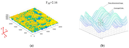
Figure 1.
3D Fractal Schematic. (a) 3D point cloud images; (b) Schematic diagram of cube coverage method.
(2) Transverse profile fractal dimension. Road texture data were acquired using the LS-40 portable 3D laser surface analyzer [41], which produced 2448 linear scan lines along the transverse direction of the lane. Each scan line consisted of 2048 height data points. The data were segmented into 2448 transverse profiles, and their fractal dimensions were computed using Equations (1) and (2). The average of these values represents the two-dimensional fractal dimension of the pavement texture in the transverse direction, denoted as F2D1, as illustrated in Figure 2.
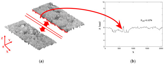
Figure 2.
Texture transverse profile diagram. (a) Schematic diagram of 3D point cloud transverse profile; (b) Schematic diagram of transverse profile texture.
(3) Longitudinal profile fractal dimension. Similarly, the 3D texture data were divided into 2048 groups along the longitudinal direction of the lane. As shown in Figure 3, the fractal dimension of each longitudinal profile was calculated, and the average value was taken as the longitudinal fractal dimension of the pavement texture, denoted as F2D2.
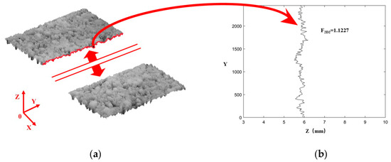
Figure 3.
Texture longitudinal profile diagram. (a) Schematic diagram of 3D point cloud longitudinal profile; (b) Schematic diagram of longitudinal profile texture.
(4) Top-view fractal dimension. To analyze the pavement texture from a top-down perspective, a 3D point cloud reconstruction model was generated and color-coded as shown in Figure 4. The RGB images were converted to grayscale by removing hue and saturation components while retaining brightness, following Equation (3). The grayscale images were then binarized using the Otsu’s maximum inter-class variance method [45], with threshold values predominantly ranging between 0.78 and 0.82, as depicted in Figure 5. Finally, the fractal dimension of the binary image was calculated using Equations (1) and (2), as shown in Figure 6. This resulting fractal dimension, denoted as FSur, characterizes the surface complexity of the pavement.
where, Gray represents the grayscale value; R, G, and B represent the red, green, and blue components of the pixel.
Figure 4.
Color rendering diagram.
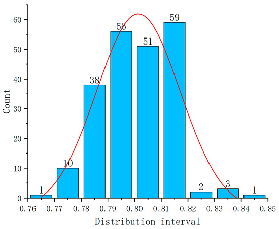
Figure 5.
Threshold frequency distribution map.
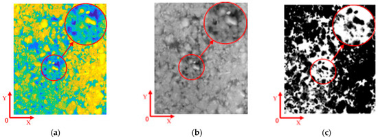
Figure 6.
Schematic Diagram for Fractal Calculation of Pavement Surface. (a) Texture surface layer cloud image; (b) Texture surface grayscale image; (c) Texture surface binary map (Fractal = 1.85).
(5) Top-segmentation-view fractal dimension. When tires contact the road surface, the actual contact area varies across different regions. As the depth within the pavement texture increases, the tire-road contact area continuously changes, resulting in certain portions of the texture that may not directly interact with the tires. This spatial variability can affect the accuracy of anti-slip performance evaluation models that rely solely on surface texture features. To address this limitation, the present study proposes dividing the pavement texture into ten equal layers along the depth direction and quantifying the geometric complexity of each layer through fractal dimension analysis. The choice of ten layers was based on previous fractal-based pavement studies [26], which demonstrated that segmentation at this scale provides a balance between capturing sufficient morphological detail and avoiding excessive redundancy.
The depth profile fractal analysis is implemented as shown in Figure 7: First, a 3D point cloud reconstruction of the pavement texture is generated. Subsequently, the texture is horizontally segmented into ten equally spaced cross-sectional layers along the depth axis. Finally, the fractal dimension of each layer’s cross-sectional profile is calculated using Equations (1) and (2). These fractal dimensions, denoted as F10% through F90%, represent the geometric complexity at successive depth intervals within the pavement texture.
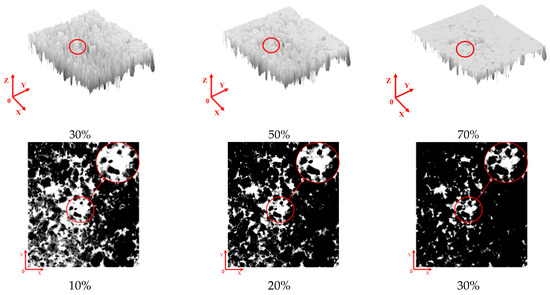
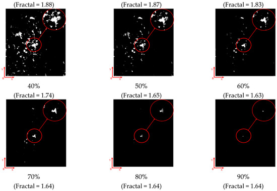
Figure 7.
Cross-section diagram of the road surface at different depths.
Statistical analysis is carried out on the obtained multi-view fractal dimension (F3D, F2D, FSur, F10% ~ F90%) and road surface temperature (T), as shown in Figure 8. The road surface temperature (T) ranges from 11.6 to 29.0 °C. The F3D is between 2.06 and 2.28, the F2D is between 1.12 and 1.13, the FSur is between 1.81 and 1.87, and the fractal dimension of other depth profiles is between 1.60 and 1.88. The spatial fractal dimension is the highest among the examined directions and differs significantly from the fractal dimensions obtained in the transverse and depth directions. This finding indicates that the spatial complexity of the pavement texture images is distinctly greater than that observed in the transverse and depth cross-sectional images. Although the fractal dimensions derived from the cross-sectional and depth directions are relatively close, their differences remain statistically significant, suggesting notable variations in texture complexity when viewed from different perspectives.
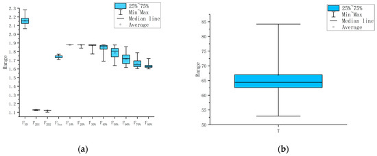
Figure 8.
Boxplot of characteristic. (a) Fractal dimension data; (b) Parallel temperature data (Put the temperatures in according to the order of each collection.).
3. Data Acquisition
3.1. Road Texture Data Collection
In this study, road texture data were acquired using the LS-40 portable 3D laser surface analyzer. The device operates based on the principle of laser triangulation, utilizing a high-definition CMOS camera in conjunction with a laser transmitter, as illustrated in Figure 9b. During data acquisition, the laser beam is projected vertically onto the road surface, while the CMOS camera captures the reflected laser light from various surface points. As the laser-camera assembly moves, the CMOS continuously records reflections over time, integrating each laser line’s data to reconstruct a three-dimensional point cloud representation of the road texture. The scanning range of the device covers a longitudinal length of 115 mm with 2448 data points and a horizontal length of 102 mm with 2048 data points, achieving a spatial accuracy of 0.05 mm. For this research, a total of 221 road texture datasets were collected, including 144 datasets from the LTPP SPS-10 asphalt pavement test section in Oklahoma, United States, and 77 datasets from asphalt pavements located around the campus of Oklahoma State University (OSU) in Stillwater.
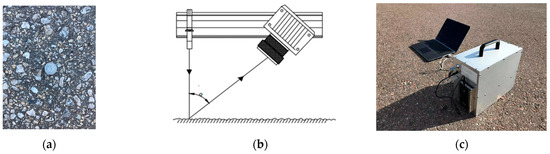
Figure 9.
Schematic diagram of road texture point cloud collection. (a) Site Map of Road Texture; (b) Laser triangulation schematic; (c) LS-40 Portable 3D Laser Surface Analyzer.
3.2. Road Texture Data Processing
During the process of scanning road texture information using the LS-40 portable 3D laser surface analyzer, there may be a small number of outliers in the collected data due to environmental and human factors. This study used the MAD [46] (median absolute deviation) method to adjust outliers in road texture data. Specifically, data points beyond the [Xmedian ± n·MAD] range were not removed but were replaced by the nearest boundary value within the range. This ensured that extreme outliers were moderated while preserving the overall data distribution and minimizing bias. Step 1: Find the median Xmedian in this set of data. Step 2: Calculate the absolute deviation of each data from the median. Step 3: Obtain the median MAD of the absolute deviation value. Last step: Determine parameter n·MAD to obtain a reasonable range of data [Xmedian − n·MAD, Xmedian + n·MAD]. The n·MAD means the n times of the MAD, which is used to construct a data range for detecting and correcting outliers, and then helping adjust the data that exceeds the range, as shown in the Equation (4).
3.3. Data Collection of Pavement Anti Slip Performance
Pavement texture data collection was accompanied by measurement of the pavement’s anti-slip performance using the Dynamical Friction Coefficient Tester (DFT), as illustrated in Figure 10. The testing process is fully automated and controlled by a computer. A torque sensor located beneath the device captures the dynamic friction coefficient of the pavement surface across a speed range from 10 to 80 km/h, which corresponds to the operational limits of the testing device.
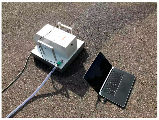
Figure 10.
Dynamic friction coefficient tester.
This study investigates the influence of vehicle speed on pavement anti-slip performance by analyzing dynamic friction coefficients measured at multiple speeds. Specifically, coefficients recorded at speeds of 10, 15, 20, 25, 30, 40, 50, 60, and 70 km/h are denoted as DFT10 through DFT70, respectively. These data were collected from two sites: the LTPP SPS-10 asphalt pavement test section and the asphalt pavement around the Oklahoma State University (OSU) Stillwater campus, as shown in Figure 11. Statistical analysis was performed using violin plots, which display key summary statistics including the minimum, maximum, median, and interquartile range (25th to 75th percentile) of the data. The violin plot’ s shape also visualizes the distribution density of the measurements. Results indicate that the distribution density of dynamic friction coefficients measured at different speeds on the same road section are relatively consistent. For this investigation, the minimum speed of 10 km/h and the maximum speed of 70 km/h were selected. These two speeds were deliberately chosen to represent extreme low-speed (urban driving) and high-speed (highway) conditions. Intermediate speeds were measured but displayed consistent trends; thus, the two representative speeds provide a simplified yet effective evaluation.
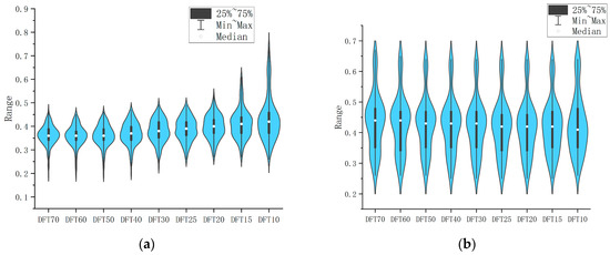
Figure 11.
In-situ friction data collection. (a) LTPP section Dynamical friction data; (b) Dynamical friction data around the OSU Stillwater campus.
4. The XGBoost Evaluation Model for Road Friction
4.1. The XGBoost Algorithm
The XGBoost (Extreme Gradient Boosting) is a state-of-the-art ensemble learning algorithm based on gradient boosting decision trees (GBDT) [47]. It is particularly well-suited for applications involving limited data, as it exhibits strong performance on small-sample datasets, making it ideal for scenarios where high-resolution pavement texture data are expensive or difficult to obtain. This study chooses decision trees as the primary learning tool for the XGBoost gradient enhancement. The basic idea is to add new decision trees continuously, and each tree will fit the residual of the previous tree’s prediction results to reduce model bias. After the final iteration is completed, the cumulative results of all trees will be the prediction results of the sample. The predicted value
is defined as:
where,
is the predicted result of sample i after the t-th iteration;
represents the prediction results of the first t − 1 trees;
denotes the model of the t-th tree.
The objective function calculation formula for the XGBoost is:
where n denotes the total amount of sample data
the Loss function, which is used to measure the error between the predicted value
and the true value
; The regularization term
is used to control the complexity of the model and avoid overfitting. The expression is:
where,
denotes the penalty coefficient of the decision tree leaf node;
indicates the regularization coefficient of L2; T and w denote the number and weight of leaf nodes in the t-th tree;
is the weight coefficient of the jth leaf node.
As shown in Figure 12, the XGBoost builds upon the fundamental concept of the second-order Taylor formula of the Loss function to enhance the accuracy of the Loss function. The model also employs multithreading to parallel search for the optimal segmentation point for each feature, thereby significantly improving the training speed.
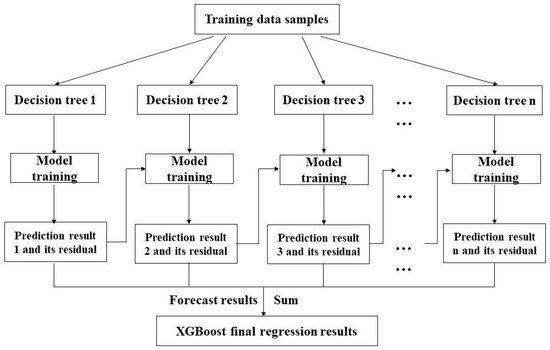
Figure 12.
Schematic diagram of the XGBoost regression algorithm principle.
4.2. The XGBoost Hyperparameter Tuning
In this study, the road texture multi-view fractal dimension (F3D, F2D, FSur, F10% ~ F90%) and road surface temperature are taken as the eigenvalues, and DFT10 and DFT70 are taken as the label data. Randomly select 70% of the data as the training set and 30% as the prediction set, and establish a regression model for road anti-slip performance based on the XGBoost algorithm.
In machine learning, hyperparameters refer to parameters that must be specified prior to the commencement of the training process. These parameters critically influence the model’s final performance. Table 1 summarizes the key hyperparameters of the XGBoost algorithm that require tuning.

Table 1.
The XGBoost hyperparameters.
This study aimed to create a reliable predictive model for the anti-slip performance of the XGBoost pavement. To achieve this, a double-layer grid search method was used to optimize the relevant parameters. The method involves two search cycles. During the first cycle, a wider search range and cycle step size are used to identify the approximate location of the optimal parameters. This helps to avoid extended search times. In the second cycle, a smaller search range is used based on the results of the first cycle. This allows for a more precise determination of the optimal parameter combination by reducing the cycle step size.
The double-layer grid search method is conducted as the following specific settings: n-estimators have a search range of 20–200 and a step size of 20. The search range of max-depth is 1–100, with a step size of 5. The search range for the learning rate is 0–1, and the step size is 0.1. The search range of reg-alpha is 0–1, and the step size is 0.1. The search range of reg-lambda is 0–1, and the step size is 0.1. By nested loop search for each parameter combination, determine the second search setting for each parameter as the search range of n-estimators is 80–100, with a step size of 1. The search range of max-depth is 1–6, with a step size of 1. The search range for the learning rate is 0.1–0.2, and the step size is 0.001. The search range of reg-alpha is 0.1–0.2, and the step size is 0.001. The search range of reg-lambda is 0.2–0.3, and the step size is 0.001.
Finally, it was determined that the model had the optimal results when n-estimators were 90, max-depth was 5, the learning rate was 0.125, reg-alpha was 0.121, and reg-lambda was 0.28. To mitigate potential overfitting, L1 and L2 regularization were applied, tree depth was restricted, and a five-fold cross-validation was conducted.
An example decision tree in the XGBoost model after hyperparameter tuning is shown in Figure 13.
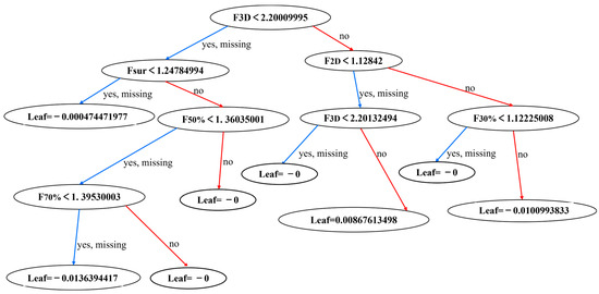
Figure 13.
Example Decision Tree in the XGBoost Model.
4.3. The Classical Prediction Model Selection for Comparison
In order to further verify the prediction performance of the XGBoost model established in this paper, this paper establishes five machine learning models based on the same eigenvalues: linear regression (LR), decision tree (DT), support vector machine (SVM), random forest (RF), BP neural network (BPNN).
4.3.1. Linear Regression Model
The linear regression algorithm is one of the most basic algorithms of machine learning. It is a Supervised learning algorithm used to predict continuous values. The multiple linear regression model can describe the relationship between the dependent variable Y and the independent variables X1, X2, X3, …, Xn.
where,
is a constant term,
(1, 2, 3, …, n) is the regression coefficient,
is the error term.
4.3.2. Decision Tree Model
Decision tree is one of the most commonly used machine learning algorithms. The establishment of the regression decision Tree model is essentially a recursive process, which recursively divides the independent variable space. Divide the feature data into N units R1, R2, …, RN, and assign a specific output value CN, to each unit. The regression decision tree model [48] is represented as:
Segmenting the feature space, with the i-th variable xi and its value s, the feature space is divided into two regions:
Furthermore, solve the following equation to obtain the optimal segmentation point s corresponding to the variable i. Repeat the above process for each region until the conditions are met, and complete the establishment of a regression decision tree.
The hyperparameter selection of the regression decision tree pavement anti-slip performance prediction model established by this research institute is shown in Table 2:
Table 2.
Decision tree hyperparameters.
4.3.3. Random Forest Model
Random forest is an ensemble learning algorithm that contains multiple decision trees. It uses the Bootstrap sampling method to randomly select data groups from the original data set to build a training sample set and repeats the process several times to create different training sample sets. For each training sample set, a node random splitting technique is used to construct a CART regression tree, and the minimum mean square deviation principle is adopted. For any partition node s corresponding to feature A, the data is divided into datasets D1 and D2, and the partition features and nodes corresponding to the minimum mean square difference between D1 and D2 and the minimum sum of mean square deviations between D1 and D2 are obtained. The specific expression [49] is as follows:
where, C1 is the sample output mean of the D1 dataset, and C2 is the sample output mean of the D2 dataset.
Finally, the mean value of the regression results of each regression tree is the final regression result of the Random forest.
where, F is the final regression result of random forest, fi is the result of the i-th regression tree, and n is the number of regression trees.
The super parameter selection of the prediction model for anti-slip performance of Random forest pavement established in this study is shown in the following Table 3:
Table 3.
Random forest hyperparameters.
4.3.4. SVM Model
SVM (Support Vector Machine) [50] is a classical machine learning algorithm, which per forms data regression in the way of Supervised learning. The support vector machine algorithm maps the original data to the high-dimensional space through nonlinear mapping to find the Hyperplane with the smallest error. The regression function established in high-dimensional space is shown in Equation (1).
Then, Lagrange function is introduced to solve ω and b, obtain the regression equation.
where,
is Lagrange operator, N is the number of support vectors, cis the penalty coefficient,
is the kernel function,
is the error term.
The hyperparameter selection of the support vector machine pavement anti-slip performance prediction model established by this research institute is shown in Table 4:
Table 4.
SVM hyperparameters.
4.3.5. BPNN Model
BPNN is a multi-layer feedforward network system that combines a large number of neurons to solve nonlinear complex problems using a gradient steepest descent learning strategy. In the process of forward transmission, the output value of each node is obtained according to the output value, weight value, threshold value, and Activation function of all nodes in the upper layer. The specific formula [51] is as follows:
where, m is the number of nodes, ω is the weight value, b is the threshold value, and f is the Activation function.
During the reverse transmission process, by continuously adjusting the weights and thresholds of the network along the steepest descent direction of the sum of relative error squares, the error in achieving the actual output and expected output of the system is reduced. The specific formula is as follows:
where, E is the Error function, d is the output layer result, δ is the learning signal.
The hyperparameter selection of the BPNN pavement anti-slip performance prediction model established by this research institute is shown in Table 5:
Table 5.
BPNN hyperparameters.
5. Result Analysis
5.1. The Pavement Texture Feature Correlation Analysis
Further, Pearson correlation analyses were performed both between and within groups on the datasets comprising multi-view fractal dimensions (F3D, F2D, FSur, F10% ~ F90%), road surface temperature, and dynamic friction coefficients. The results are presented as follows. As shown in Figure 14, no significant linear correlations were observed among the multi-view fractal dimensions, road surface temperature, and dynamic friction coefficients. This lack of linear association underscores the necessity of employing machine learning algorithms capable of capturing and explaining nonlinear relationships to more effectively investigate the underlying connections between the selected features and pavement friction. Moreover, Figure 15 reveals that, with the exception of certain depth-profile fractal dimensions, the fractal correlation coefficients between adjacent depth layers are relatively high, reflecting the continuity inherent in road texture. In contrast, the linear correlation coefficients among other features generally remain below 0.6. These findings indicate that the multi-view fractal dimensions and road surface temperature independently characterize distinct aspects of pavement texture complexity, justifying their combined use for comprehensive modeling of anti-slip performance.
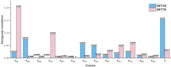
Figure 14.
Intergroup correlation between comprehensive fractal dimension and pavement friction coefficient.
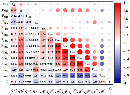
Figure 15.
Intra-group correlation of model characteristics (The left column shows the ranked order of feature importance. The right column presents SHAP (Shapley additive explanations) value distributions across samples. The numbers in the squares indicate the relative contribution scores of each feature. The circle size reflects the magnitude of influence on the model’s prediction.).
5.2. The Friction Prediction Results of the XGBoost Model
In this study, the coefficient of determination (R2) and root-mean-square error (RMSE) were selected as evaluation metrics to assess the predictive accuracy of the XGBoost model. The R2 value ranges from 0 to 1, with values closer to 1 indicating better model fit, while a smaller RMSE indicates higher prediction accuracy. Regression validation of the dynamic friction coefficient was performed using the hyperparameter-optimized model, with results summarized in Table 6 and illustrated in Figure 16. As shown, the model achieved R2 values of 0.80 for DFT10 and 0.82 for DFT70, with RMSE values below 0.05 in both cases, demonstrating its effectiveness in capturing the relationship between multi-view fractal dimensions and dynamic friction coefficient while maintaining high accuracy.
Table 6.
The XGBoost model prediction evaluation indicators.
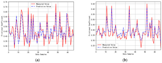
Figure 16.
Prediction results of pavement anti-slip performance (with error bars indicating ±1 standard deviation). (a) 10 km/h; (b) 70 km/h.
5.3. The Performance Comparison Between the XGBoost and Other Machine Learning Algorithms
The performance of the XGBoost are compared with that of the LR, DT, RF, SVM, and BPNN models. Based on the R2 results shown in Figure 17 and Figure 18, which compare six algorithms at both low (10 km/h) and high (70 km/h) vehicle speeds, the XGBoost model exhibits the highest predictive accuracy. As shown in Table 7: Traditional approaches such as LR model and DT model demonstrate limited generalization on the test sets (LR: R2 = 0.35 at 10 km/h, 0.44 at 70 km/h; DT: R2 = 0.68 and 0.65), while the BPNN model yields moderate performance (R2 = 0.50 at 10 km/h, 0.60 at 70 km/h). The ensemble and kernel-based methods-RF model (R2 = 0.71 at 10 km/h, 0.77 at 70 km/h) and the SVM model (R2 = 0.61 and 0.78)-offer improvements but still fall short of the XGBoost’s results. The XGBoost model not only achieves superior R2 values in both training and testing phases but also maintains an optimal balance between fit quality and generalization, underscoring its robustness and efficacy in modeling the nonlinear relationships between multi-view texture features and pavement friction across varying speeds.
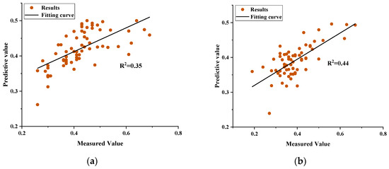
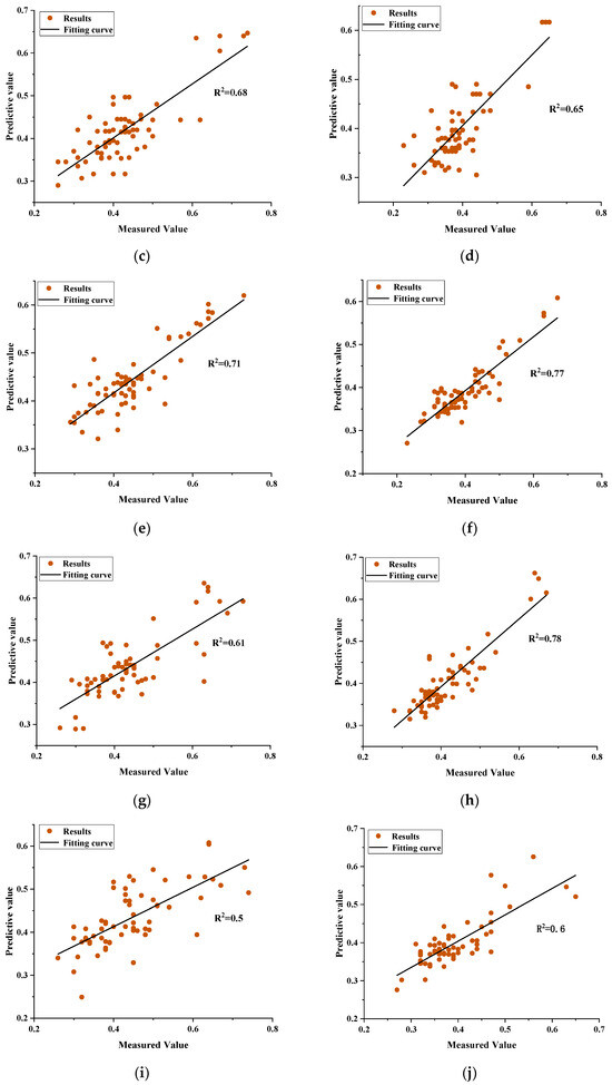
Figure 17.
Prediction results of the adopted machine learning models. (a) Linear regression model for DFT10; (b) Linear regression model for DFT70; (c) Decision tree model for DFT10; (d) Decision tree model for DFT70; (e) Random forest model for DFT10; (f) Random forest model for DFT70; (g) SVM model for DFT10; (h) SVM model for DFT70; (i) BPNN model for DFT10; (j) BPNN model for DFT70.
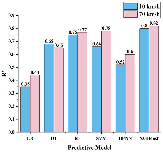
Figure 18.
Comparison Chart of Different Prediction Models R2.
Table 7.
Prediction R2 results for contrast models.
5.4. The Model Features Importance Analysis
The XGBoost model can determine the degree of influence of features on prediction results through feature importance analysis. Its evaluation idea is to calculate the importance of each feature in a single tree of the model and then take the average of all trees. The specific calculation process is shown in Equations (23) and (24).
where,
denotes the importance of a feature in a single tree; L − 1 is the number of non-leaf nodes in the tree; Vt represents the selected features during internal node t splitting;
is the reduction in square loss after splitting the internal node t;
is the importance of features in the model; M is the number of trees in the model.
This study evaluates the feature importance within the XGBoost model for predicting pavement anti-slip performance based on multi-view fractal dimensions, with results illustrated in Figure 19. It is evident that across both low- and high-speed conditions, the features F3D, F2D1, F2D2, FSur, and surface temperature (T) exert a substantial influence on the model. A more detailed breakdown indicates that F3D ranked the highest, followed by F2D2 at low speed and F2D1 + FSur at high speed. Surface temperature consistently showed strong influence, while deeper segmentation fractals contributed moderately (scores 50–80). Among these, F3D demonstrates the greatest impact on model predictions, reflecting the comprehensive spatial complexity of the road texture. In contrast, the other fractal features represent more localized or specific texture characteristics, accounting for their relatively lower importance. Surface temperature (T) also plays a significant role, primarily due to the necessity of temperature correction when interpreting friction coefficient measurements [52]. As temperature corrections were not applied in the preliminary stages of this study, temperature remains a critical factor influencing the target friction coefficient within the model. Furthermore, under slow-sliding conditions, the longitudinal profile fractal dimension (F2D2) has a pronounced effect on the model, whereas under fast-sliding conditions, transverse profile fractal (F2D1) and top-view fractal (FSur) features exhibit heightened importance, with scores exceeding 100. Additionally, the variable influence of cross-sectional fractal dimensions at different depth layers on the dynamic friction coefficient prediction under varying speeds suggests that pavement texture features at distinct depths contribute differently to anti-slip performance depending on the vehicle speed.
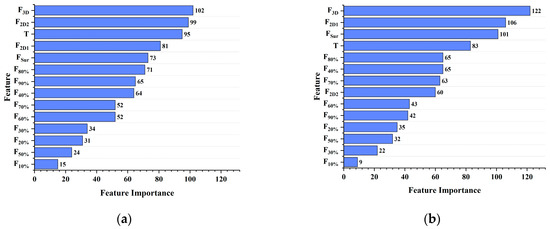
Figure 19.
Importance of the XGBoost model features. (a) 10 km/h; (b) 70 km/h.
Concurrently, as shown in Figure 20, the random forest model, whose predictive performance ranks second only to that of the XGBoost model for pavement anti-slip evaluation, was also subjected to feature importance analysis. The results indicate that F3D exerts the greatest influence under both low- and high-speed conditions. Additionally, F2D1 plays a more prominent role during fast sliding scenarios, whereas F2D2 is more influential in slow sliding states, consistent with the findings observed in the XGBoost model. However, the relative importance of other features differs markedly from those identified by the XGBoost model, with several features contributing minimally and exhibiting negligible impact on the model’s predictive outcomes.
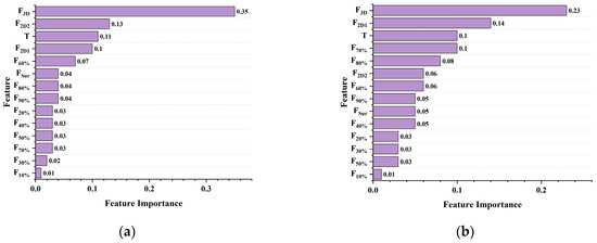
Figure 20.
Importance of RF model features. (a) 10 km/h; (b) 70 km/h.
In summary, the spatial morphology of the texture, cross-sectional texture characteristics, fractal dimensions of profiles at varying depths, and road surface temperature collectively govern the anti-slip performance of pavement surfaces.
6. Conclusions
(1) In this study, an LS-40 portable three-dimensional surface analyzer with an accuracy of 0.05 mm was used to collect road texture data, and the complexity of road texture was comprehensively characterized by multi-view fractal dimension. The fractal feature indicators of F3D, F2D1, F2D2, FSur, and F10%~F90% texture were proposed from the space, cross-section, and depth directions, respectively, improving the fractal characterization method of road texture under various spatial perspectives.
(2) For evaluating road friction, the dynamic friction coefficients measured at 10 km/h and 70 km/h were employed to represent low- and high-speed conditions, respectively. Analysis of the multi-view fractal characteristics, road surface temperature, and dynamic friction data revealed no direct linear correlation among these variables. Nevertheless, each feature independently contributes to describing the complexity of the pavement texture.
(3) By integrating multi-view fractal dimension features-capturing pavement texture complexity across spatial, cross-sectional, and depth dimensions-with road surface temperature, we developed a robust the XGBoost-based regression model for friction prediction. A two-stage grid search was used to optimize model hyperparameters, yielding a well-calibrated structure capable of learning from high-dimensional, nonlinear feature spaces.
(4) The model achieved high predictive accuracy, with R2 values of 0.80 and 0.82 at speeds of 10 km/h and 70 km/h, respectively. These results validate the effectiveness of the proposed multi-view fractal + the XGBoost framework in characterizing texture-friction relationships. Unlike prior approaches that utilize either standard texture indices or single-view fractal parameters, our method provides a more granular, scale-aware assessment of anti-slip performance and enables the potential transition from contact-based testing to efficient, non-contact friction evaluation.
(5) Through analysis of the XGBoost model for pavement anti-slip performance evaluation, it was determined that multiple factors significantly influence anti-slip behavior. These factors encompass the spatial morphology of texture, cross-sectional texture properties, fractal characteristics of profiles at varying texture depths within the multi-view fractal dimension framework, as well as road surface temperature. Furthermore, the relative importance of these factors was found to vary depending on the vehicle speed regime.
In addition, although 221 datasets were used in this study—which is relatively large for high-resolution pavement texture research—the sample size is still limited compared to typical machine learning applications. The higher training R2 values compared to testing results suggest possible mild overfitting, which we have mitigated through cross-validation and regularization. However, several limitations remain: (i) the dataset was collected from only two locations in Oklahoma, which may restrict the generalizability of the findings; (ii) only surface temperature was considered as an environmental factor, while humidity, rainfall, and seasonal cycles were not included; and (iii) only two representative speeds were analyzed. Therefore, future studies should expand to larger geographic regions, employ larger-scale datasets, incorporate multiple environmental variables, and investigate a wider range of vehicle speeds to further validate and generalize the proposed framework.
Author Contributions
Conceptualization, Y.P.; methodology, Y.P.; software and formal analysis, Z.Z.; investigation, Y.P.; resources, Q.J.L. and G.Y.; data curation, X.Y.; writing—original draft preparation, J.K.; writing—review and editing, J.K. and X.Y.; visualization, Z.Z.; supervision, Y.P.; project administration, L.K.; funding acquisition, Y.P. All authors have read and agreed to the published version of the manuscript.
Funding
This research was funded by “Key Laboratory Open Foundation of New Technology for Construction of Cities in Mountain Area, China, grant number LNTCCMA-20250116”, “Chongqing Technology Innovation and Application Development Project: Sichuan—Chongqing Science and Technology Innovation Cooperation Program, grant number CSTB2024TIAD-CYKJCXX0004”, “National Natural Science Foundation, China, grant number 52208425” and “Chongqing Chengtou Infrastructure Construction Co., Ltd. joint technology research project, grant number CQCT-JS-SC-GC-2024-0076”.
Data Availability Statement
The datasets generated or analyzed during the current study are not available due to confidentiality agreements and cannot be shared.
Conflicts of Interest
Author Xinyi Yu was employed by Chongqing Loke Highway Maintenance Co., Ltd. Author Zhengqi Zhang was employed by Hangzhou Jiaotong Engineering Design Co., Ltd. The remaining authors declare that the research was conducted in the absence of any commercial or financial relationships that could be construed as a potential conflict of interest.
References
- Chen, J.; Yuan, X.W.; Liu, Q.; Zhao, C.; Zhou, R.Y.; Huang, J.L. Identifying Texture and Friction of Asphalt Pavement Surface with Optimized Close-Range Photogrammetry Method. J. Test. Eval. 2023, 51, 3081–3094. [Google Scholar] [CrossRef]
- Zhong, J.T.; Zhang, J.; Huang, K.; Blankenship, P.; Ma, Y.T.; Xiao, R.; Huang, B.S. An investigation of texture-friction relationship with laboratory ring-shaped asphalt mixture specimens via close-range photogrammetry. Constr. Build. Mater. 2024, 442, 137508. [Google Scholar] [CrossRef]
- Liu, X.; Luo, H.; Chen, C.; Zhu, L.; Chen, S.; Ma, T.; Huang, X. A technical survey on mechanism and influence factors for asphalt pavement skid-resistance. Friction 2024, 12, 845–868. [Google Scholar] [CrossRef]
- Li, S.; Hu, J.Y.; Tan, Y.Q.; Xiao, S.Q.; Han, M.Z.; Li, S.; Li, J.L.; Wang, W. A review of non-contact approach for pavement skid resistance evaluation based on texture. Tribol. Int. 2024, 196, 109737. [Google Scholar] [CrossRef]
- Li, Y. Fractal Dimension Estimation for Color Texture Images. J. Math. Imaging Vis. 2019, 62, 37–53. [Google Scholar] [CrossRef]
- Chen, X.H.; Wang, D.W. Fractal and spectral analysis of aggregate surface profile in polishing process. Wear 2011, 271, 2746–2750. [Google Scholar] [CrossRef]
- Villani, M.M.; Scarpas, A.; de Bondt, A.; Khedoe, R.; Artamendi, I. Application of fractal analysis for measuring the effects of rubber polishing on the friction of asphalt concrete mixtures. Wear 2014, 320, 179–188. [Google Scholar] [CrossRef]
- Li, L.; Wang, K.C.P.; Luo, W. Pavement Friction Estimation Based on the Heinrich/Klüppel Model. Period. Polytech. Transp. Eng. 2016, 44, 89–96. [Google Scholar] [CrossRef][Green Version]
- Legrand, P.; Sandu, C.; Taheri, S.; Motamedi, M. Characterization of Road Profiles Based on Fractal Properties and Contact Mechanics. Rubber Chem. Technol. 2017, 90, 405–427. [Google Scholar] [CrossRef]
- Lu, J.; Pan, B.; Che, T.; Sha, D. Discrete element analysis of friction performance for tire-road interaction. Ind. Lubr. Tribol. 2020, 72, 977–983. [Google Scholar] [CrossRef]
- Zhong, K.; Sun, M.; Liu, Z.; Zheng, K. Research on dynamic evaluation model and early warning technology of anti-sliding risk for the airport pavement. Constr. Build. Mater. 2020, 239, 117820. [Google Scholar] [CrossRef]
- Liu, C.; Zhan, Y.; Deng, Q.; Qiu, Y.; Zhang, A. An improved differential box counting method to measure fractal dimensions for pavement surface skid resistance evaluation. Measurement 2021, 178, 109376. [Google Scholar] [CrossRef]
- Wang, K.; Li, Y.; Zhu, Y.; Xiang, H.; Lu, G. Research on Characteristics of Macrotexture for Colored Anti-Skid Coating on Pavement Based on Fractal Theory. Transp. Res. Rec. J. Transp. Res. Board 2022, 2676, 129–140. [Google Scholar] [CrossRef]
- Ueckermann, A.; Wang, D.; Oeser, M.; Steinauer, B. A contribution to non-contact skid resistance measurement. Int. J. Pavement Eng. 2015, 16, 646–659. [Google Scholar] [CrossRef]
- Zelelew, H.; Khasawneh, M.; Abbas, A. Wavelet-based characterisation of asphalt pavement surface macro-texture. Road Mater. Pavement Des. 2014, 15, 622–641. [Google Scholar] [CrossRef]
- Kane, M.; Rado, Z.; Timmons, A. Exploring the texture–friction relationship: From texture empirical decomposition to pavement friction. Int. J. Pavement Eng. 2014, 16, 919–928. [Google Scholar] [CrossRef]
- Ueckermann, A.; Wang, D.; Oeser, M.; Steinauer, B. Calculation of skid resistance from texture measurements. J. Traffic Transp. Eng. 2015, 2, 3–16. [Google Scholar] [CrossRef]
- Li, Q.; Yang, G.; Wang, K.C.P.; Zhan, Y.; Wang, C. Novel Macro- and Microtexture Indicators for Pavement Friction by Using High-Resolution Three-Dimensional Surface Data. Transp. Res. Rec. J. Transp. Res. Board 2017, 2641, 164–176. [Google Scholar] [CrossRef]
- Panagouli, O.K.; Kokkalis, A.G. Skid resistance and fractal structure of pavement surface. Chaos Solitons Fractals 1998, 9, 493–505. [Google Scholar] [CrossRef]
- Kokkalis, A.G.; Panagouli, O.K. Fractal Evaluation of Pavement Skid Resistance Variations. II: Surface Wear. Chaos Solitons Fractals 1998, 9, 1891–1899. [Google Scholar] [CrossRef]
- Hartikainen, L.; Petry, F.; Westermann, S. Frequency-wise correlation of the power spectral density of asphalt surface roughness and tire wet friction. Wear 2014, 317, 111–119. [Google Scholar] [CrossRef]
- Mahboob Kanafi, M.; Tuononen, A.J. Top topography surface roughness power spectrum for pavement friction evaluation. Tribol. Int. 2017, 107, 240–249. [Google Scholar] [CrossRef]
- Kokkalis, A.G.; Tsohos, G.H.; Panagouli, O.K. Consideration of Fractals Potential in Pavement Skid Resistance Evaluation. J. Transp. Eng. 2002, 6, 128. [Google Scholar] [CrossRef]
- Zhang, H.; Chen, X.; Xu, G.; Huang, D.; He, J. Effect of Surface Texture Variation on Skid Resistance of Asphalt Pavement. In Proceedings of the China International Conference on Transportation and Infrastructure (CICTP), Nanjing, China, 6–8 July 2019; pp. 987–998. [Google Scholar] [CrossRef]
- Lin, L.; Wang, K.C.P.; Li, Q. Geometric texture indicators for safety on asphalt concrete pavements with 1 mm 3D laser texture data. Int. J. Pavement Res. Technol. 2016, 9, 49–62. [Google Scholar] [CrossRef]
- Ding, S.; Wang, K.C.P.; Yang, E.; Zhan, Y. Influence of effective texture depth on pavement friction based on 3D texture area. Constr. Build. Mater. 2021, 287, 123002. [Google Scholar] [CrossRef]
- Tan, Q.; Xu, X.; Liang, H. Physiological Big Data Mining Through Machine Learning and Wireless Sensor Networks. Int. J. Distrib. Syst. Technol. 2023, 14, 1–12. [Google Scholar] [CrossRef]
- Krizhevsky, A.; Sutskever, I.; Hinton, G.E. ImageNet classification with deep convolutional neural networks. Commun. ACM 2017, 60, 84–90. [Google Scholar] [CrossRef]
- Rasol, M.; Schmidt, F.; Ientile, S. FriC-PM: Machine Learning-based road surface friction coefficient predictive model using intelligent sensor data. Constr. Build. Mater. 2023, 370, 130567. [Google Scholar] [CrossRef]
- Yu, M.; Liu, S.; You, Z.; Yang, Z.; Li, J.; Yang, L.; Chen, G. A prediction model of the friction coefficient of asphalt pavement considering traffic volume and road surface characteristics. Int. J. Pavement Eng. 2023, 24, 2160451. [Google Scholar] [CrossRef]
- Liu, C.; Li, J.; Gao, J.; Yuan, D.; Gao, Z.; Chen, Z. Three-dimensional texture measurement using deep learning and multi-view pavement images. Measurement 2021, 172, 108828. [Google Scholar] [CrossRef]
- Yang, G.; Li, Q.J.; Zhan, Y.; Fei, Y.; Zhang, A. Convolutional Neural Network-Based Friction Model Using Pavement Texture Data. J. Comput. Civ. Eng. 2018, 32, 1943–5487. [Google Scholar] [CrossRef]
- Zhan, Y.; Li, J.Q.; Yang, G.; Wang, K.C.P.; Yu, W. Friction-ResNets: Deep Residual Network Architecture for Pavement Skid Resistance Evaluation. J. Transp. Eng. Part B Pavements 2020, 146, 04020027. [Google Scholar] [CrossRef]
- Ban, I.; Deluka-Tibljaš, A.; Ružić, I. Skid Resistance Performance Assessment by a PLS Regression-Based Predictive Model with Non-Standard Texture Parameters. Lubricants 2024, 12, 23. [Google Scholar] [CrossRef]
- Yu, M.; Zhang, R.; Tang, O.; Jin, D.; You, Z.; Zhang, Z. Construction and optimization of asphalt pavement texture characterization model based on binocular vision and deep learning. Measurement 2025, 248, 116946. [Google Scholar] [CrossRef]
- Massimo, B.; Davide, M.; Mattia, N.; Francesco, Z. Machine Learning for industrial applications: A comprehensive literature review. Expert Syst. Appl. 2021, 175, 114820. [Google Scholar] [CrossRef]
- Mohammad, M.; Mohammad, R.T. Investigation of Polyamide 12 Powder Cooling Process under Natural Convection via Porous Medium, Non-porous Medium, and Experimental Approaches. J. Mater. Eng. Perform. 2024, 34, 9352–9373. [Google Scholar] [CrossRef]
- Sanghyun, W.; Jongchan, P.; Joon-Young, L.; In So, K. CBAM: Convolutional Block Attention Module. In Proceedings of the Proceedings of the European Conference on Computer Vision (ECCV), Munich, Germany, 8–14 September 2018; pp. 3–19. [Google Scholar] [CrossRef]
- Mao, Y.H.; He, C.; Jiang, L.Z. Postearthquake train operation safety assessment model based on machine learning. Intell. Transp. Infrastruct. 2024, 3, liae017. [Google Scholar] [CrossRef]
- Tang, Y.Z.; Qian, Y.; Yang, E.H. Weakly supervised convolutional neural network for pavement crack segmentation. Intell. Transp. Infrastruct. 2022, 1, liac013. [Google Scholar] [CrossRef]
- Yang, G.; Yu, W.; Li, Q.J. Random Forest-Based Pavement Surface Friction Prediction Using High-Resolution 3D Image Data. J. Test. Eval. A Multidiscip. Forum Appl. Sci. Eng. 2021, 2, 49. [Google Scholar] [CrossRef]
- Zhan, Y.; Liu, C.; Deng, Q.S.; Feng, Q.; Qiu, Y.J.; Zhang, A.; He, X.L. Integrated FFT and XGBoost framework to predict pavement skid resistance using automatic 3D texture measurement. Measurement 2022, 188, 110638. [Google Scholar] [CrossRef]
- Yan, Y.; Ran, M.; Sandberg, U.; Zhou, X.; Xiao, S. Spectral Techniques Applied to Evaluate Pavement Friction and Surface Texture. Coatings 2020, 10, 424. [Google Scholar] [CrossRef]
- Zhang, Y.H.; Zhou, H.W.; Xie, H.P. Improved cubic covering method for fractal dimensions of a fracture surface of rock. Chin. J. Rock Mech. Eng. 2005, 24, 3192–3196. [Google Scholar]
- Onur, T.O. Improved Image Denoising Using Wavelet Edge Detection Based on Otsu’s Thresholding. Acta Polytech. Hung. 2022, 19, 79–92. [Google Scholar] [CrossRef]
- Park, J.W.; Moon, Y.S. Robust estimation of target scale by removing outlier motion vectors using MAD. Electron. Lett. 2015, 51, 691–693. [Google Scholar] [CrossRef]
- Chen, T.; Guestrin, C. XGBoost: A Scalable Tree Boosting System. In Proceedings of the 22nd ACM SIGKDD International Conference on Knowledge Discovery and Data Mining, San Francisco, CA, USA, 13–17 August 2016; Association for Computing Machinery: New York, NY, USA, 2016; pp. 785–794. [Google Scholar] [CrossRef]
- Krzywinski, M.; Altman, N. Classification and regression trees. Nat Methods 2017, 14, 757–758. [Google Scholar] [CrossRef]
- Friedman, J.H. Greedy function approximation: A gradient boosting machine. Ann. Stat. 2001, 29, 1189–1232. [Google Scholar] [CrossRef]
- Cortes, C.; Vapnik, V. Support-vector networks. Mach. Learn. 1995, 20, 273–297. [Google Scholar] [CrossRef]
- Hastie, T.; Tibshirani, R.; Friedman, J. The Elements of Statistical Learning: Data Mining, Inference, and Prediction, 2nd ed.; Springer: New York, NY, USA, 2009. [Google Scholar] [CrossRef]
- Eng, M.; Tighe, S.L. Effect of Short-term and Long-term Weather on Pavement Surface Friction. Int. J. Pavement Res. Technol. 2010, 3, 295. [Google Scholar]
Disclaimer/Publisher’s Note: The statements, opinions and data contained in all publications are solely those of the individual author(s) and contributor(s) and not of MDPI and/or the editor(s). MDPI and/or the editor(s) disclaim responsibility for any injury to people or property resulting from any ideas, methods, instructions or products referred to in the content. |
© 2025 by the authors. Licensee MDPI, Basel, Switzerland. This article is an open access article distributed under the terms and conditions of the Creative Commons Attribution (CC BY) license (https://creativecommons.org/licenses/by/4.0/).