Predicting Asphalt Pavement Friction by Using a Texture-Based Image Indicator

Abstract

Pavement skid resistance is of vital importance for road safety. The objective of this study is to propose and validate a texture-based image indicator to predict pavement friction. This index enables pavement friction to be predicted easily and inexpensively using digital images, with predictions correlated to Dynamic Friction Tester (DFT) measurements. Three different types of asphalt surfaces (Dense-Grade Asphalt Concrete, Open-Grade Friction Course, and Chip Seal) were evaluated subject to various tire polishing cycles. Images were taken with corresponding friction coefficients obtained using DFT in the laboratory. The aggregate protrusion area is proposed as the indicator. Statistical models are established for each asphalt surface type to correlate the proposed indicator with friction coefficients. The results show that the adjusted R-squared values of all relationships are above 0.90. Compared to other image-based indicators in the literature, the proposed image indicator more accurately reflects the changes in pavement friction with the number of polishing cycles, proving its cost-effective use for considering pavement friction in the mix design stage.

1. Introduction

Skid resistance, the force generated when a tire, prevented from rotating, slides along the pavement surface, is a key indicator for quality management and routine maintenance. Accurately measuring skid resistance ensures that the required friction is achieved before the pavement is put into use, which is crucial for driving safety. Inadequate skid resistance can lead to high risks, such as sliding, rear-end collisions, and longer braking distances, potentially causing traffic accidents [1]. Additionally, efficient measurement techniques are needed to quickly assess whether the pavement in use provides sufficient friction for vehicles [2], facilitating routine management by transportation departments. Furthermore, skid resistance also indicates the degree of wear and aging of the pavement, making accurate prediction a valuable guide for pre-maintenance.

Traditional methods for measuring skid resistance typically involve direct friction measurements. These include field tests, high-speed and laboratory tests, as well as low-speed approaches. High-speed methods encompass four distinct skid resistance measurement techniques, all of which require attaching a trailer or a wheel to a vehicle and measuring the friction force at the interface between a locked, sliding wheel and the wet pavement surface [3,4]. Laboratory tests often employ the British Pendulum Tester (BPT) and the Dynamic Friction Tester (DFT). These tests measure pavement friction by assessing the loss of kinetic energy in a sliding pendulum or rotating disk when it contacts the roadway surface, converting this loss to a frictional force [5,6]. Although direct friction measurements provide a clear reflection of the pavement’s actual skid resistance, they are limited to spot measurements and are not suitable for large-scale assessments. Additionally, these methods are heavily influenced by testing vehicles and experimental conditions, necessitating the involvement of skilled technicians. Consequently, researchers have recently proposed new methods for measuring skid resistance.

Recently, novel methods for non-contact measurement of pavement friction have been studied. Pérez-Acebo et al. [7] developed two skid resistance prediction models for an entire road network. These machine learning models consider multiple factors affecting skid resistance and can assist road management departments in predicting future skid resistance. However, this method requires identifying pavement materials and calculating traffic volume, and it does not provide real-time measurements. Roy et al. [8] proposed image-based indicators of microtexture and macrotexture for pavement to predict initial skid resistance. Nonetheless, the predicted skid resistance may not accurately reflect the pavement’s condition after years of traffic, as skid resistance can deteriorate over time. Du et al. [9] utilized the signal processing technique of wavelet decomposition to characterize pavement texture but failed to establish a correlation model with friction. Yang et al. [10] employed a deep learning network, FrictionNet-V, based on three-dimensional (3D) laser imaging technology to evaluate skid resistance. However, the extensive and complex information in the raw 3D data can lead to overfitting issues and poor result stability [11,12], especially when the training sample data are limited and the network layers are deep. Additionally, the laser equipment required demands high memory for data storage and is expensive [13].

The challenges of friction measurements still exist. Traditional direct friction measurement methods suffer from poor repeatability and low correlation between various equipment indicators. Additionally, these methods can only provide point-based friction predictions, resulting in discontinuous outcomes. Among the novel non-contact methods, texture-based approaches estimate pavement friction by calculating characteristic indicators, but the correlation between these indicators and skid resistance is relatively low. Despite the fact that deep learning has been proven to be a reliable method for estimating pavement friction, its effectiveness is constrained by the quality and size of the training dataset. Inconsistencies and inadequacies in the true value data can confuse the deep learning network during training, leading to inadequate accuracy and low portability to other scenarios [14].

To address these limitations, this study explores a cost-effective and non-intrusive way of using image processing methods to evaluate skid resistance of pavement surface. First, digital images and friction coefficients are collected from asphalt slabs with different surface texture patterns. Then, a series of image processing algorithms are developed. Finally, an interpretable image indicator representing the selected texture feature is proposed to predict friction with good accuracy. Compared to image-based indicators developed in previous studies, the established method can more effectively reflect the changes in pavement friction with varying wear levels, making it potentially applicable to field detection of pavement friction under repeated traffic loading.

The novelty of this approach lies in its use of a single, interpretable texture indicator (aggregate protrusion area) derived from 2D digital images captured with a smartphone, processed through straightforward algorithms as described in Section 3.1. Unlike Roy et al. [8], which focused on initial skid resistance using multiple texture indicators, this method captures friction changes across wear cycles, achieving high correlation (R²_adj > 0.90, Section 4.1) for multiple pavement types. In contrast to 3D-surface-based methods like Yang et al. [10], which rely on costly laser equipment and complex data prone to overfitting, this approach uses cost-effective 2D imaging, reducing equipment costs and computational complexity while maintaining robust performance across varying wear conditions. This simplicity and portability enhance its applicability for real-time field assessments, addressing the limitations of both prior image-based and 3D-surface-based methods.

2. Laboratory Experiment and Data Collection

2.1. Friction Data Acquisition

Laboratory tests were conducted on three asphalt surfaces: Dense-Grade Asphalt Concrete (DGAC), Open-Grade Friction Course (OGFC), and Chip Seal, with one slab prepared for each surface type due to experimental constraints. These surfaces were selected to represent a range of macrotexture characteristics relevant to image-based texture analysis for friction prediction: DGAC for moderate macrotexture typical of highways, OGFC for high macrotexture and drainage, and Chip Seal for very high macrotexture due to exposed aggregates, ideal for skid resistance studies. Stone Mastic Asphalt (SMA) was not included due to its macrotexture similarity to DGAC and the resource limitations that restricted this study to three distinct pavement types.

Friction coefficients were measured using the Dynamic Friction Tester (DFT), with a single measurement per slab per wear level due to limited experimental conditions, conducted at a controlled temperature of 20–25 °C to ensure consistency. The DFT is a portable instrument designed to measure the friction value of pavement surfaces, allowing for the recording of friction coefficients at various speeds. Despite the lack of repeated measurements, the high correlation between friction coefficients and the proposed image indicator (R²_adj > 0.90, Section 4.1) suggests reliable data. Simulated trafficking was performed using a three-wheel polisher, following ASTM E1911-09a [15], with a platform applying a 68 kN load via three 2.80/2.40-4 tires (35 psi pressure), driven by a motor at 60 cycles per minute. The polishing process was conducted along a circular wheel path with a diameter of 28.5 cm, matching the DFT test circle.

The DGAC mix was designed with a nominal maximum aggregate size (NMAS) of 12.5 mm, following a dense-graded mix design with a bitumen content of 5.0% by weight and a target air void content of 4–7%. The OGFC mix had an NMAS of 9.5 mm, characterized by a high air void content (18–22%) and a bitumen content of 6.0%, designed to enhance drainage and friction. The Chip Seal surface consisted of a single-layer application of 10 mm NMAS aggregates embedded in a 1.2 kg/m² emulsion binder, providing a high-texture surface for improved skid resistance. All test specimens were constructed using crushed granite aggregates, selected for their common use in asphalt pavements. No significant aggregate loss was observed during the simulated trafficking process for any of the tested surfaces.

The friction data were collected at a constant speed of 40 km/h and recorded after the vehicle tire had rotated 0 k, 50 k, 90 k, 150 k, 300 k, 390 k, 450 k, and 500 k times on the samples. On the same sample, friction can vary slightly at different positions due to the effects of water, load, and other factors [16]. Therefore, all pavement slabs were kept dry prior to conducting the experiment. Additionally, external conditions such as temperature and humidity were kept consistent during data collection to minimize the impact of environmental factors. The evolution of friction coefficients with polishing cycles is shown in Figure 1 for three different asphalt surfaces.

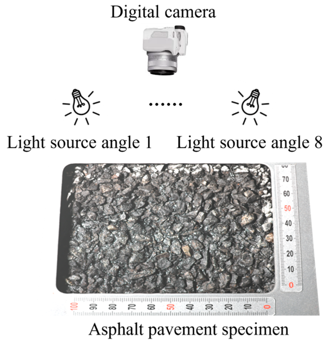
2.2. Digital Image Acquisition

Images of the pavement surface were captured when the polisher had abraded the surface to the set number of rotations. The images were taken using a smartphone camera (e.g., iPhone 12 Pro) with a 12 MP sensor upscaled to a resolution of 350 dpi for both horizontal and vertical dimensions and a pixel size of 6000 × 4000, saved in JPEG format. The camera was hand-held at an approximate distance of 30–50 cm from the test surface to capture the region of interest (ROI) alongside the reflective silver calibration board. Adjustable LED lights with a color temperature of approximately 5500 K were used to illuminate the pavement surface, allowing for consistent lighting across 8 different angles (Figure 2). Each image contained 24,000,000 pixels, with each pixel consisting of three values (R, G, B). Considering that the quality of pavement image texture is mainly determined by factors such as lighting conditions, camera position, and other variables [17,18,19], at least 10 images with 8 different light source angles were collected for each level of wear to evaluate the practicality of the proposed image processing methods. The images were taken with the corresponding friction values and polishing cycles; some examples are shown in Figure 3.

3. Analysis Methodology

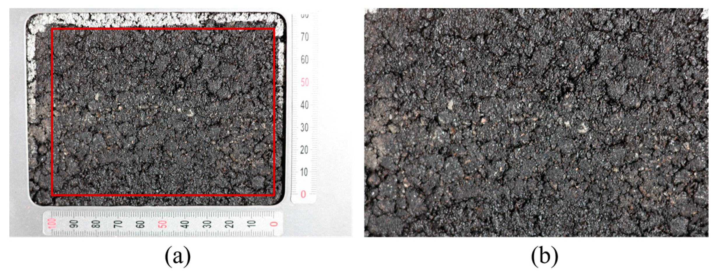
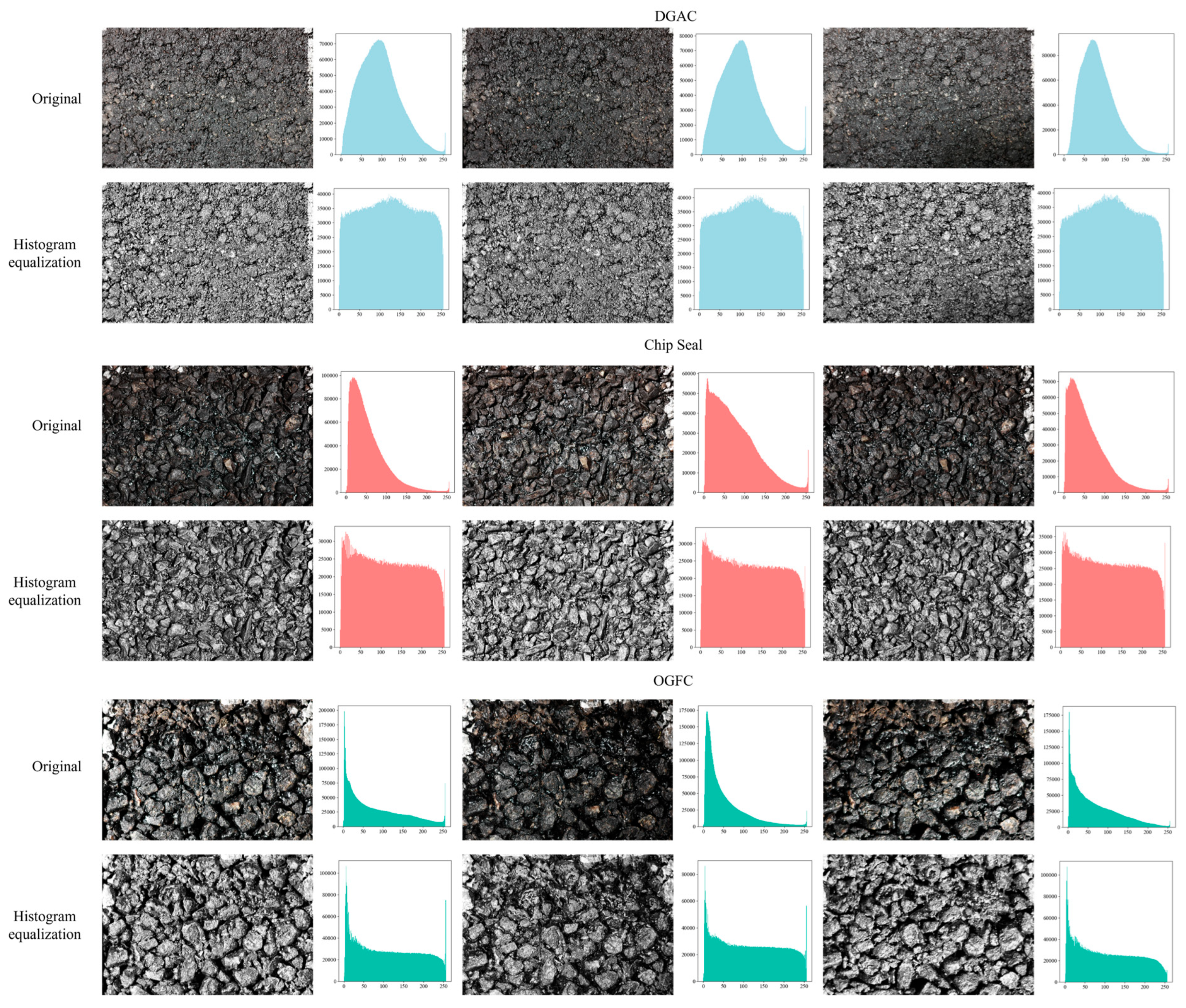
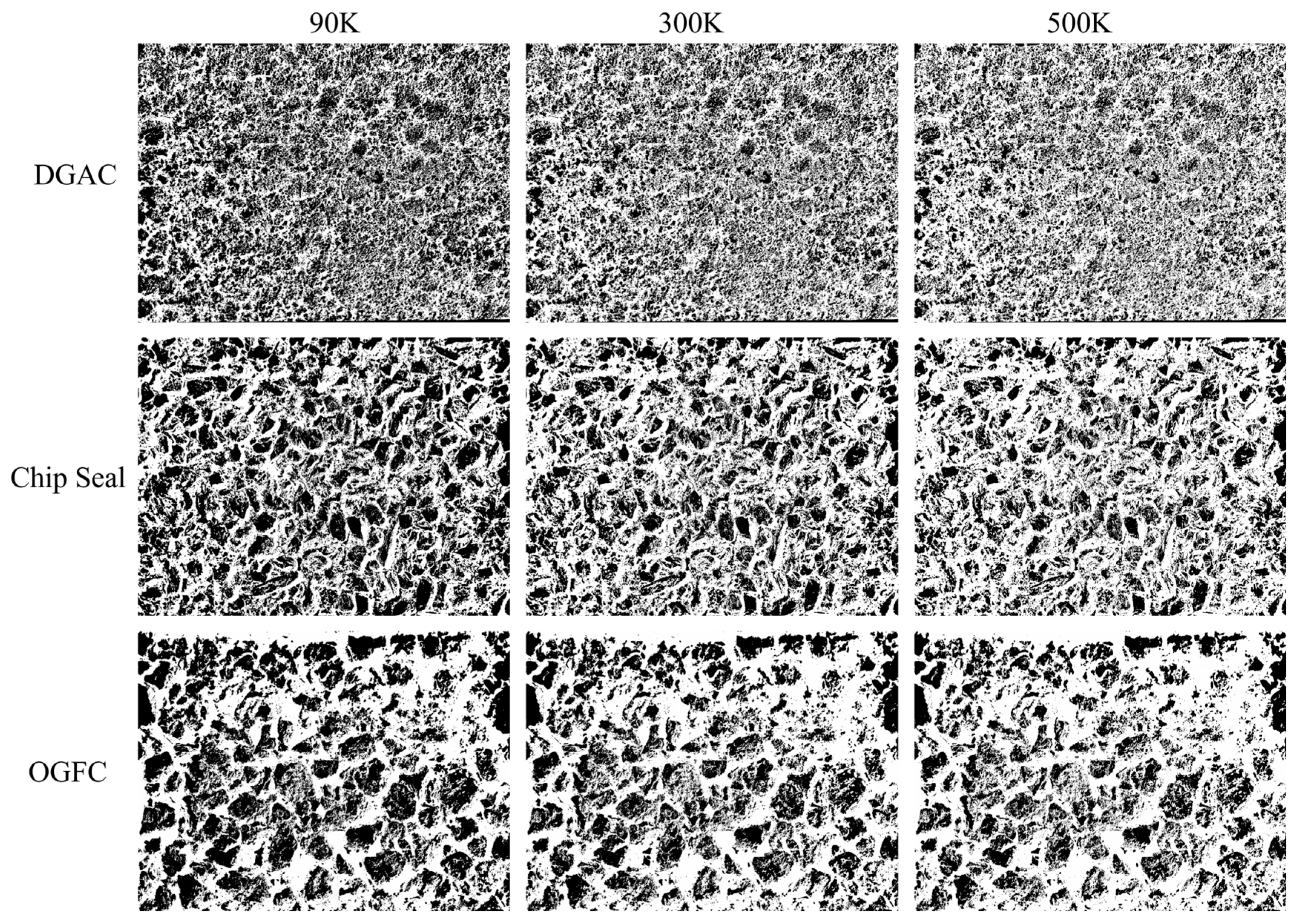
3.1. Image Preprocessing

A series of image processing algorithms were performed to obtain the binary image and extract the image-based texture feature for friction prediction, as shown in Figure 4. For each level of wear, 10 images were selected from one asphalt slab per surface type (DGAC, OGFC, and Chip Seal), across 8 polishing cycles, resulting in a total of 240 images (3 surfaces × 1 slab × 8 wear levels × 10 images) to evaluate the texture features.

First, a region of interest (ROI) sized 100 mm × 75 mm is selected and cropped from the color image (as shown within the red box in Figure 5a) using an image processing program, with no physical scaling rulers employed. The reflective silver calibration board, included in the images, serves as a visual reference to identify the ROI boundaries, excluding non-pavement areas such as the board itself and white marks that do not represent the true brightness values of the pavement. In practice, users of this method can adjust the camera’s height above the ground according to the area of the pavement they wish to measure, potentially eliminating the need for cropping. As the equipment used in this study does not have a fixed position, slight variations in the distance between the lens and the sample occur during image capture. To ensure consistency, each cropped ROI is programmatically adjusted to a standardized pixel dimension of 3400 × 2550, corresponding to 100 mm × 75 mm at 350 dpi, as shown in Figure 5b. The image resolution of 0.0294 × 0.0294 mm meets the required precision for pavement skid resistance analysis [20]. Next, the adjusted RGB image is converted to an 8-bit grayscale image using the weighted average method [21,22,23]. The calculation method is expressed in Equation (1) as follows:

Gray = 0.299 × R + 0.587 × G + 0.114 × B

(1)

where Gray is the resulting grayscale value, and R, G, and B are the red, green, and blue channel values of the original image, respectively [24,25,26].

In practice, shooting devices occasionally generate unqualified images due to the impact of external light, surface reflectance properties, and other factors [27,28,29]. As shown in Figure 6, three representative images are selected from the image sets of each mixture type to demonstrate these effects. The original photos show the imaging results under different lighting conditions and material types. For instance, the third original photo in the DGAC category illustrates that when the light incidence angle is not perpendicular to the pavement, part of the pavement appears clear while another part is shrouded in shadows. Similarly, the second original photo in the OGFC category demonstrates that when the pavement color is darker and the light source is tilted, it only illuminates a small portion of the pavement. However, in the first original photo of the OGFC category, even if the lighting angle is orthogonal, the reflective properties of the pavement can cause the aggregates to exhibit uneven brightness. Since the subsequent threshold selection step performs binarization based on pixel brightness values, the brightness distribution of such unqualified images needs to be adjusted to ensure consistency for determining a uniform threshold for each type of mixture.

Typically, histogram equalization techniques are used to redistribute the grayscale values of an image to address such issues [30]. However, traditional methods may result in the loss of local details, especially in images with varying brightness [31,32,33]. Adaptive Histogram Equalization (AHE) mitigates this by dividing the image into multiple small blocks (referred to as ‘tiles’ or ‘grids’) and applying histogram equalization to each tile individually [34]. The boundaries between tiles are then smoothed using bilinear interpolation. Building on AHE, Contrast Limited Adaptive Histogram Equalization (CLAHE) introduces the concept of contrast limiting [35]. This involves clipping the histogram of each tile, with the clip limit being a predefined parameter that determines the maximum number of pixels for any single grayscale level [36]. This prevents excessive contrast enhancement and avoids amplifying noise. As shown in Figure 6, CLAHE is applied to the grayscale image by transforming the values to achieve a brightness distribution where all values are equally probable. The original images under different lighting conditions show varying gray distributions. After applying CLAHE, the gray levels of the same type of pavements are distributed equally. This eliminates discrepancies in the binarization results caused by varying lighting conditions, leading to more consistent texture feature values. Additionally, this algorithm enhances the local contrast of the image, making the details more pronounced.

For subsequent image segmentation tasks, the histogram-equalized image needs to be denoised. Due to its smooth and artifact-free characteristics, the Gaussian filter is widely used [37,38]. A two-dimensional (2D) Gaussian filter is chosen to smooth the surface. This filter smooths the image through a convolution operation, with the convolution kernel generated by the 2D Gaussian function G(x,y). The calculation method is defined in Equation (2) as follows:

$$G(x,y)={\displaystyle \frac{1}{2\pi {\sigma }^2}}{e}^{-{\displaystyle \frac{x^2+y^2}{2{\sigma }^2}}}$$

(2)

where (x,y) represents coordinates relative to the center of the Gaussian kernel, and σ is the standard deviation that determines the width of the Gaussian distribution. When the filter smooths the image, pixels in different positions in the neighborhood are given different weights. Pixels farther from the center of the Gaussian kernel (filter window) have smaller weights [39]. Thus, more of the overall gray distribution characteristics of the image are retained compared to median and arithmetic mean filters [40].

3.2. Texture Feature Extraction

The contact area between the tire and the road surface significantly impacts the skid resistance of the pavement [41]. To extract the area metric, we can assume the existence of a frictional contact surface. Textures above this surface will come into contact with the rubber and generate friction, while textures below this surface will have little to no contact with the rubber. If 3D laser data of the pavement are available, the position of this contact surface relative to the pavement can be calculated, and then the actual contact area can be predicted using methods such as machine learning [42]. However, these methods require collecting a large amount of data to train the machine learning model [43,44]. Additionally, regression models need to be established to achieve the final goal of predicting friction [45], making the entire prediction process computationally expensive and time-consuming.

Due to the significant impact of the aggregate’s morphological characteristics on the surface properties of asphalt pavement [46] and the fact that aggregates with sharp, angular shapes offer better skid resistance [47,48,49], it is concluded that the more protruding aggregates the pavement has, the stronger the friction the tire will experience. Therefore, even though 2D images cannot provide depth information like 3D point cloud data and we cannot calculate the absolute elevation of the contact surface to extract realistic contact area, we can still quantify texture features based on the difference in grayscale information between the protruding parts of the aggregates and both the non-protruding parts of the aggregates and the asphalt. Since the grayscale distribution of images of the same mixture type is adjusted for consistency in the preprocessing step, and the grayscale contrast between the protruding aggregates and other parts of the pavement is enhanced, an appropriate binarization algorithm can determine a unified threshold for each pavement type to effectively segment the grayscale image, as shown in Figure 7, retaining only the aggregates protruding from the surface (marked in black) and removing other regions by treating them as background (marked in white). For the sake of convenience in the text, this textural feature will be referred to as “Area”.

In the field of image processing, researchers have proposed various binarization methods, which are mainly divided into global thresholding methods and local (adaptive) thresholding methods [50,51,52]. This study opts for the global thresholding method, primarily because the defined protruding part of the aggregates is relative to the entire pavement rather than relative to its surrounding small area. Consequently, a uniform threshold should be applied to the entire image instead of determining the threshold at each pixel location based on the pixel value distribution of its neighborhood block. Representative global thresholding methods like Otsu’s Method [53] and IsoData [54] have demonstrated robust performance in image segmentation. Considering the characteristics of the grayscale distribution of the analyzed images, this paper selects the IsoData method, which adapts better to complex gray-level distributions and is less sensitive to noise. Otsu’s method is not chosen because it is more suitable for bimodal gray-level histograms and performs poorly with unimodal or multimodal distributions [55,56].

Specifically, the IsoData method selects an initial threshold T0 (the mid-value of the grayscale range). The image is then split into a low grayscale part (grayscale value ≤ T) and a high grayscale part (grayscale value > T). The mean grayscale value μ_L for the low grayscale part (Equation (3)) and the mean grayscale value μ_H for the high grayscale part (Equation (4)) are calculated. The threshold is updated according to Equation (5). The difference between the new threshold T_new and the old threshold T is compared. If the difference is less than the preset tolerance ε, the threshold is considered to have converged, and the final threshold T_final is used to convert the grayscale image into a binary image (Equation (6)). If not, the new threshold T_new is set as the current threshold T, and the iterative calculation continues.

$${\mu }_L={\displaystyle \frac{1}{N_L}}{\displaystyle \sum _{i=1}^{N_L}{I}_i}$$

(3)

$${\mu }_H={\displaystyle \frac{1}{N_H}}{\displaystyle \sum _{i=N_L+1}^{N_L+N_H}{I}_i}$$

(4)

$$T_{new}={\displaystyle \frac{{\mu }_L+{\mu }_H}{2}}$$

(5)

$$I(x,y)=\left\{\begin{array}{l}1, \mathrm{if} I_{gray}(x,y)>T_{final}\\ 0, \mathrm{if} I_{gray}(x,y)\le T_{final}\end{array}\right.$$

(6)

where N_L and N_H are the total number of pixels in the low and high grayscale parts, respectively. I_i represents the grayscale value, and I(x, y) is the pixel value of the binary image at the coordinates (x, y).

As previously mentioned, by adjusting the grayscale distribution of each type of mixture to be consistent, the thresholds derived from this algorithm for various pavement images are relatively similar. The thresholds set for the images of DGAC, Chip Seal, and OGFC surfaces are 127, 124, and 115, respectively. Users should note that due to differences between field operation conditions and the experimental setup in this study, such as lighting conditions during photography and the color of the mixtures, the thresholds used in this paper should be further calibrated for practical use. The primary purpose of this study is to provide an imaging-based methodology for quickly estimating pavement friction. More extensive data can be utilized to further train and refine the models established in this study.

Some of the segmentation results are shown in Figure 7. For the same type of mixture, the area of the protruding aggregates decreases after more polishing cycles, corresponding to a reduction in the actual friction [57]. Given that the number of pixels along the width of the image is 2550 and the corresponding actual length is 75 mm, it is straightforward to calculate the actual area size of the black parts in the binarized image.

Table 1. Examples of texture feature calculation results.

Pavement Type	Area (mm2)	Friction	Polishing Cycles (k)
DGAC	2795.53	0.54	50
	2611.88	0.52	90
	2427.15	0.50	150
	……
Chip Seal	2547.03	0.67	50
	2122.78	0.63	90
	1856.24	0.60	150
	……
OGFC	2518.15	0.38	50
	2634.07	0.36	90
	2456.65	0.36	150
	……

presents some of the calculated results of the Area indicators along with their corresponding true friction values and the number of polishing cycles. It is evident that the Area on the same type of pavement shows a regular linear change with friction. However, the pattern for any one type of pavement cannot be directly applied to others. Therefore, it is necessary to develop separate models for different pavement types. Detailed experimental results can be found in Section 4. More variables are not introduced because overfitting is a common issue in multiple linear regression models when the sample size is small relative to the number of predictors [58,59]. Additionally, capturing the nonlinear relationships between the predictors and DFT is challenging with limited data [60,61,62].

3.3. Other Image-Based Indicators from Literature

Various image-based indicators have been proposed to directly or indirectly predict the pavement friction. This study selects three indicators that have demonstrated relatively good predictive performance in previous research experiments. These indicators are used to establish relationships with DFT friction to evaluate the effectiveness and superiority of the proposed texture feature.

Valikhani et al. [63] proposed an image-based metric called Aggregate Ratio (AR), defined by Equation (7):

AR = A_aggregate/A_surface

(7)

where A_surface represents the area of the surface, which is equal to the entire image size, and A_aggregate represents the complete particle area of aggregates. The selection of image thresholds in their study is based on the grayscale value differences between the aggregate surface and the black asphalt. In contrast, our study determines thresholds based on the differences in grayscale values between the protruding parts of the aggregates and both the non-protruding parts of the aggregates and the asphalt.

Roy et al. [8] utilized the wavelet transform method to extract image texture features. By decomposing the image into sub-images of different resolutions and detail images containing high-frequency details, detail coefficients are extracted from the high-frequency detail images. The energy features are obtained by calculating the arithmetic mean of the squared values of the detail coefficients at each decomposition level. Based on these energy features, a macrotexture indicator called the Surface Macrotexture Index (SMI) is proposed to determine the skid resistance of newly constructed road surfaces.

Wan et al. [64], based on the brightness distinction between convex and concave parts, used the maximum entropy method to segment the concave areas of the pavement. They then employed the Fractal Dimension (FD) to characterize the concave distribution characteristics (CDC) of pavements, establishing a strong correlation with texture depth (TD) and mean texture depth (MTD) obtained through the sand patch method. The FD is calculated using the box-counting method, as defined in Equation (8).

$$FD=-\underset{\epsilon \to 0}{\lim }{\displaystyle \frac{\log (N(\epsilon ))}{\log (\epsilon )}}$$

(8)

where ε represents the changeable box size and Nε(P) represents the minimum number of an n-dimensional box. The calculation processes of all the above indicators are reproduced according to the previous literature [8,63,64], where the calculation details can be found.

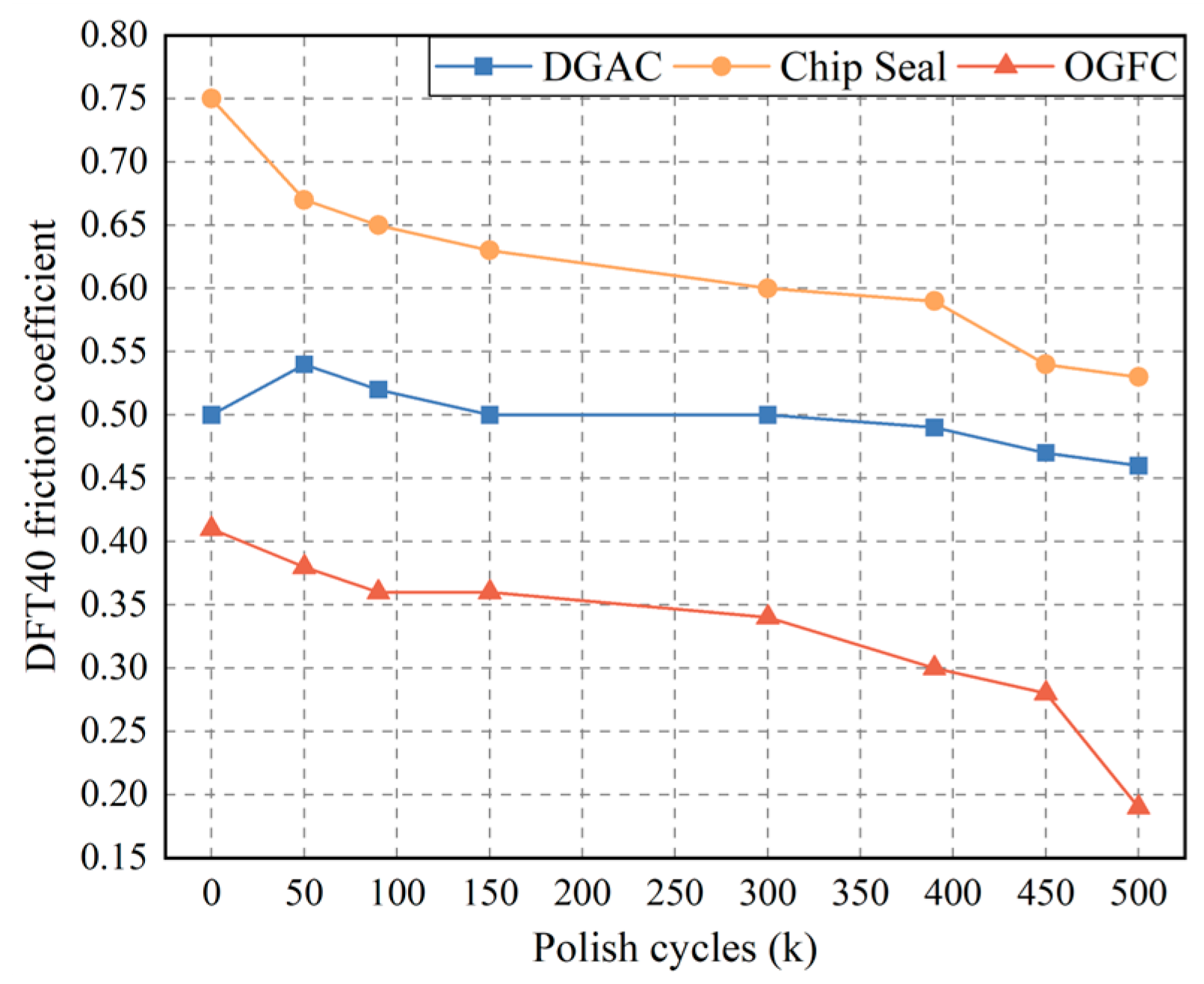
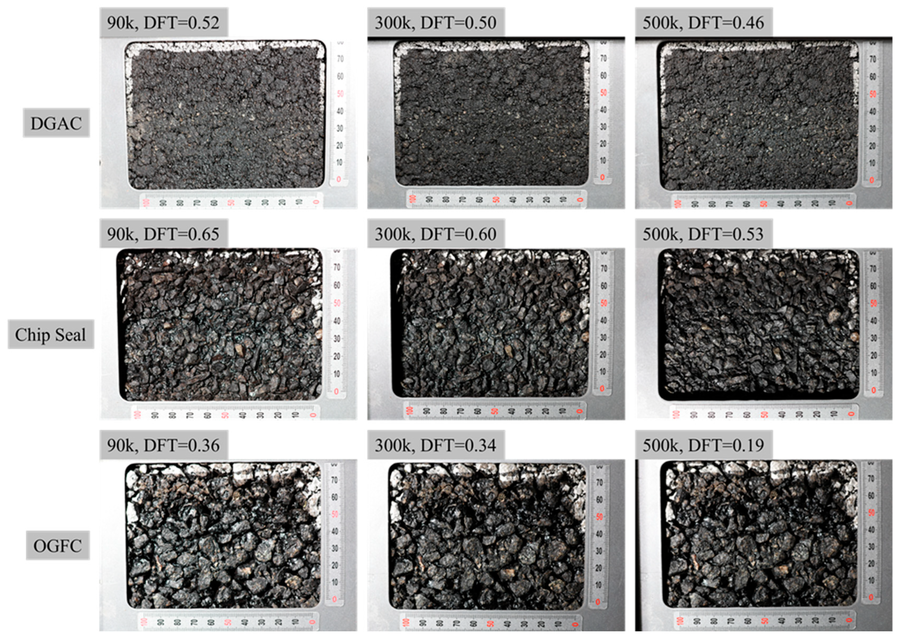
4. Results and Discussion

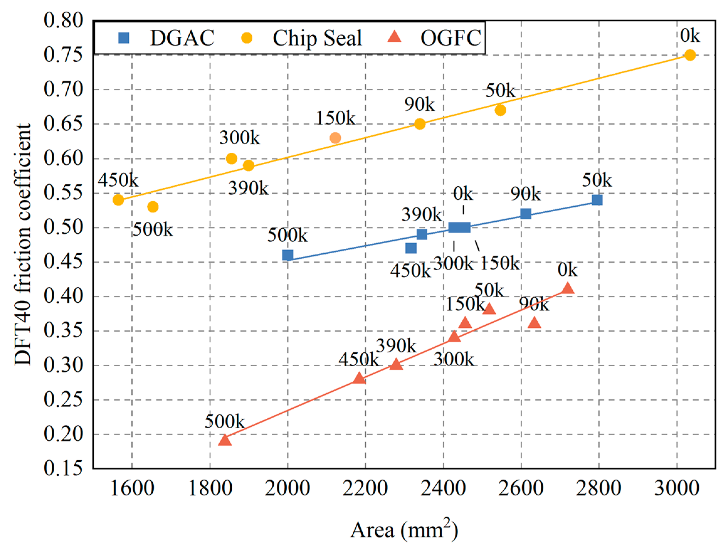
4.1. Evaluation of Proposed Image Indicator

This study is conducted on a laptop with an AMD Ryzen 9 5900 HX central processing unit (CPU). Data from DGAC, Chip Seal, and OGFC surfaces in the dataset are used to build the relationship models. As shown in Figure 8, the Area determined from image analysis is compared to DFT data to develop separate models for different pavement types. Most of the data points are found close to the line of equality, indicating that the proposed indicator is valid [65,66]. As the number of times the tires polish the pavement increases, friction is expected to reduce as the macrotexture diminishes and the area of protruding textures decreases. However, as documented in [67], the friction of the pavement can slightly increase in the early stages of grinding. At this stage, if one touches the pavement with a finger, the texture appears rougher and potentially more abrasive. Except for DGAC pavement, our data do not reflect this friction change trend in the early stages, primarily because the intervals between the polishing cycles when measuring the friction were not small enough. Research indicates that the macrotexture of aggregate surfaces significantly impacts the skid resistance of pavement, and this macrotexture is primarily controlled by aggregate gradation parameters [68]. Generally, mixtures with a larger nominal maximum aggregate size (NMAS) tend to provide better skid resistance [69]. As shown in Figure 8, Chip Seal exhibits higher surface friction compared to DGAC. However, this evaluation criterion is not absolute, as the friction of OGFC is lower than that of DGAC.

Table 2. The established friction prediction models for various types of pavements.

Pavement Type	Pearson’s Correlation	R2	R2adj	Regression Models
DGAC	0.9620	0.9255	0.9130	DFT = 0.2396 + 1.0632 × 10−4 Area
Chip Seal	0.9851	0.9704	0.9655	DFT = 0.3151 + 1.4331 × 10−4 Area
OGFC	0.9782	0.9569	0.9498	DFT = −0.2504 + 2.4260 × 10−4 Area

summarizes the indicators of the linear regression equations, and the calculation formulas for the three selected indicators are shown in Equations (9)–(11):

$$r={\displaystyle \frac{{\displaystyle \sum (y_i-\overline{y})}({\widehat{y}}_i-\overline{\widehat{y}})}{\sqrt{{{\displaystyle \sum (y_i-\overline{y})}}^2{({\widehat{y}}_i-\overline{\widehat{y}})}^2}}}$$

(9)

$$R^2=1-{\displaystyle \frac{{{\displaystyle \sum (y_i-{\widehat{y}}_i)}}^2}{{{\displaystyle \sum (y_i-\overline{y})}}^2}}$$

(10)

$$R_{adj}^2=1-({\displaystyle \frac{1-R^2}{n-p-1}}\times (n-1))$$

(11)

where r represents the Pearson Correlation Coefficient, which measures the linear relationship between two variables. R² is the Coefficient of Determination (COD) [70,71,72,73], representing the proportion of variance in the dependent variable that is predictable from the independent variable. R²_adj is the Adjusted Coefficient of Determination, which adjusts the R² value based on the number of predictors in the model, providing a more accurate measure of the model’s explanatory power [74,75,76]. y_i are the observed values, and ${\widehat{y}}_i$ are the predicted values. $\overline{y}$ is the mean of the observed values, and $\overline{\widehat{y}}$ is the mean of the predicted values. n is the number of observations, and p is the number of predictors [77,78,79,80].

The adjusted R² values for all three models are greater than 0.90, indicating significant relationships [81,82,83,84]. The different slopes of the three regression lines suggest that the rate of friction reduction varies among different pavement types under the same wear conditions. For example, the friction reduction in OGFC pavements is significantly higher than that of DGAC pavements. This information can guide the selection of materials for pavements with different functions. For instance, DGAC material is a better choice for constructing long-lasting pavements.

Despite similar aggregate protrusion areas across the three surfaces, as shown in Figure 8, differences in DFT40 values are observed, primarily due to variations in mix design and surface texture. The Chip Seal surface, with a 10 mm NMAS and a single-layer application of aggregates embedded in a 1.2 kg/m² emulsion binder, exhibits a positive texture with exposed aggregates, resulting in higher DFT40 values (e.g., intercept of 0.3151 in Table 2) due to enhanced macrotexture and direct aggregate–tire contact. In contrast, DGAC, with a 12.5 mm NMAS and a dense–graded structure (4–7% air voids), has a smoother surface with less pronounced macrotexture, leading to lower DFT40 values (intercept of 0.2396). OGFC, with a 9.5 mm NMAS and high air void content (18–22%), features a porous, negative texture that enhances drainage but reduces aggregate–tire contact, resulting in the lowest DFT40 values (negative intercept of −0.2504). As all surfaces used crushed granite aggregates, aggregate type does not contribute to these differences. These variations in NMAS, binder properties, and positive/negative texture explain the distinct friction trends observed in Figure 8, highlighting the influence of surface-specific characteristics on skid resistance beyond the aggregate protrusion area alone.

Regarding the sources of error in the proposed prediction method, the following four possibilities are identified: First, the limited number of samples (240 images total, one slab per surface type, Section 3.1) leads to limited accuracy in prediction models and restricts the implementation of training/test splits or cross-validation [85], which could increase the risk of overfitting. To mitigate this, simple linear regression models were used, as they are less prone to overfitting compared to complex models [86], and experimental conditions were tightly controlled, including consistent temperature (20–25 °C, Section 2.1) and standardized image capture with eight lighting angles processed via CLAHE (Section 2.2 and Section 3.1) to ensure uniform brightness. The high R²_adj values (>0.90) across three distinct pavement types with varied macrotextures (DGAC, OGFC, and Chip Seal) suggest robustness of the models despite the lack of a separate test set. Second, obtaining the actual friction values of the pavement under high-speed conditions is challenging, which also results in some inevitable prediction errors. Third, the threshold selection method for image binarization is not perfect, resulting in some texture features being ignored or overly enhanced. Fourth, the single DFT measurement per wear level (Section 2.1) introduces potential variability, though the strong correlation (R²_adj > 0.90) mitigates this concern. Future studies with larger datasets will incorporate training/test splits or k-fold cross-validation to enhance model generalizability and further validate the proposed image-based indicator.

4.2. Comparison of Accuracy for Different Image-Based Indicators

The same image dataset was used to calculate three image-based indicators in the literature (AR, SMI, and FD) and evaluate their accuracy for friction prediction. Figure 9 shows the correlation between the AR calculation results and DFT friction obtained using linear regression. Compared to the proposed indicator, the R² values of the three fitted lines are quite low, indicating they do not effectively capture the trend of the data points [87,88,89]. This is because, using the threshold-based method from the literature, the area of exposed aggregates on the same pavement does not significantly change with different polishing cycles. The minor variations in AR values for the same mix under different polish cycles are due to the contrast and brightness of the images not being perfectly adjusted to the same levels. In other words, the proposed indicator can better simulate the interaction between aggregates and tires as they undergo repeated polishing, providing a more accurate prediction of friction. The AR indicator might be more suitable for evaluating the initial friction of different types of pavements, offering a simple and effective means for approximate friction assessment. However, due to the limited number of mix types included in this study, we did not establish a predictive model to verify the potential applicability of this indicator.

Figure 10 shows the results of fitting SMI and DFT using linear equations for different mixture types. The adjusted R² values for the DGAC and Chip Seal models are both higher than 0.90, indicating a significant relationship between SMI and DFT in this case [90,91,92], and SMI performs similarly to the proposed indicator. Due to the wavelet transform method’s superior noise resistance compared to the threshold segmentation method, it allows for more accurate extraction of macrotexture features. Therefore, extracting the SMI to represent pavement friction is even more effective, as demonstrated in the case of DGAC. The adjusted R² value between SMI and DFT is 0.9481, while the adjusted R² value between Area and DFT is 0.9130. However, the adjusted R² value for the OGFC model is only 0.8061, indicating a weaker correlation between SMI and DFT [93,94,95], which is worse than the proposed indicator. Considering that friction is influenced by both macrotexture and microtexture, this indicates that the contribution of microtexture to OGFC friction cannot be ignored. The macrotexture indicator (SMI) fails to fully capture this influence because wavelet transform involves complex multi-scale analysis, which may lead to microtexture information loss or the introduction of errors during feature extraction. In contrast, threshold segmentation, which directly processes the grayscale values of the images, is relatively simple and can better preserve the original information.

Figure 11 illustrates the relationship between FD and DFT for various mixtures. According to the adjusted R² values of the models, using FD to predict the friction of Chip Seal performs similarly to the proposed indicator but performs worse for DGAC and OGFC. This is because FD can capture the complexity and irregularity of surfaces at different scales, making it excellent at representing the texture of Chip Seal pavements, which have rough surfaces with significant multi-scale irregularities. For DGAC pavements, which have relatively regular and smooth textures, the FD does not provide additional useful information. In this case, a simple threshold selection method can more effectively capture the key surface features. For OGFC, a porous hydrophobic material, image-based indicators fail to capture the internal pore structure of such pavements. Compared to concave distribution characteristics (CDC), the protruding aggregates have a more direct and significant impact on friction performance. Additionally, the FD method requires the selection and tuning of multiple parameters, such as the choice of wavelet basis and the number of decomposition levels. Incorrect parameter selection can lead to poor prediction results [96,97,98]. In contrast, the proposed method is relatively easy to implement, requiring only the selection of an appropriate threshold based on the type of mixture.

5. Conclusions

This study proposed a texture-based image indicator for characterizing surface texture features and predicting pavement friction. The proposed image preprocessing techniques effectively mitigate the effects of varying lighting conditions and camera heights during photography. Modeling results indicate that the aggregate protrusion area, extracted using a threshold selection algorithm, establishes a strong correlation with DFT-measured friction coefficients. The adjusted R² values of friction prediction models exceed 0.90 for each of three different types of pavement surfaces. Comparative analysis demonstrates that the proposed image indicator outperforms other image-based indices, particularly in accurately reflecting changes in pavement friction with polishing cycles.

It is proved that the proposed image indicator and models can be used to evaluate pavement friction during the mix design phase. However, it is important to note that this study developed prediction models for each type of asphalt mixture or surface treatment separately, and the established method may not be applicable to pavement surface types not included in the dataset for model development. Future work is needed to evaluate the feasibility of the image indicator for network application using images taken from the moving vehicle and friction measurements from the skid tester in the field.

References

1. Grande, Z.; Castillo, E.; Mora, E.; Lo, H.K. Highway and road probabilistic safety assessment based on Bayesian network models. Comput. Aided Civ. Infrastruct. Eng. 2017, 32, 379–396. [Google Scholar] [CrossRef]
2. Čelko, J.; Kováč, M.; Kotek, P. Analysis of the pavement surface texture by 3D scanner. Transp. Res. Procedia 2016, 14, 2994–3003. [Google Scholar] [CrossRef]
3. Antle, C.E.; Wambold, J.; Henry, J.; Rado, Z. International PIARC Experiment to Compare and Harmonize Texture and Skid Resistance Measurement. PIARC Tech. Commitee Surf. Charact. C 1995, 1, 1995. [Google Scholar]
4. Rezaei, A.; Masad, E.; Chowdhury, A.; Harris, P. Predicting asphalt mixture skid resistance by aggregate characteristics and gradation. Transp. Res. Rec. 2009, 2104, 24–33. [Google Scholar] [CrossRef]
5. Rado, Z.; Yager, T.; Wambold, J.; Hall, J. Guide for Pavement Friction; The National Academies Press: Washington, DC, USA, 2006. [Google Scholar]
6. Asi, I.M. Evaluating skid resistance of different asphalt concrete mixes. Build. Environ. 2007, 42, 325–329. [Google Scholar] [CrossRef]
7. Pérez-Acebo, H.; Gonzalo-Orden, H.; Findley, D.J.; Rojí, E. A skid resistance prediction model for an entire road network. Constr. Build. Mater. 2020, 262, 120041. [Google Scholar] [CrossRef]
8. Roy, N.; Mondal, P.G.; Kuna, K.K. Image-based indices of aggregates for predicting the initial skid resistance of bituminous pavements. Constr. Build. Mater. 2023, 400, 132776. [Google Scholar] [CrossRef]
9. Du, Y.; Weng, Z.; Li, F.; Ablat, G.; Wu, D.; Liu, C. A novel approach for pavement texture characterisation using 2D-wavelet decomposition. Int. J. Pavement Eng. 2022, 23, 1851–1866. [Google Scholar] [CrossRef]
10. Yang, G.; Zhang, A.A.; Wang, K.C.; Li, J.Q.; Liu, W.; Liu, Y. Deep-learning based non-contact method for assessing pavement skid resistance using 3D laser imaging technology. Int. J. Pavement Eng. 2023, 24, 2147520. [Google Scholar] [CrossRef]
11. Dan, H.-C.; Lu, B.; Li, M. Evaluation of asphalt pavement texture using multiview stereo reconstruction based on deep learning. Constr. Build. Mater. 2024, 412, 134837. [Google Scholar] [CrossRef]
12. Feng, C.; Bačić, B.; Li, W. SCA-LSTM: A Deep Learning Approach to Golf Swing Analysis and Performance Enhancement. In Proceedings of the International Conference on Neural Information Processing, Auckland, New Zealand, 2–6 December 2024; pp. 72–86. [Google Scholar]
13. Dan, H.-C.; Yan, P.; Tan, J.; Zhou, Y.; Lu, B. Multiple distresses detection for Asphalt Pavement using improved you Only Look Once Algorithm based on convolutional neural network. Int. J. Pavement Eng. 2024, 25, 2308169. [Google Scholar] [CrossRef]
14. Wang, Y.; Yu, B.; Zhang, X.; Liang, J. Automatic extraction and evaluation of pavement three-dimensional surface texture using laser scanning technology. Autom. Constr. 2022, 141, 104410. [Google Scholar] [CrossRef]
15. ASTM E1911-09a; Standard Test Method for Measuring Paved Surface Frictional Properties Using the Dynamic Friction Tester. ASTM: West Conshohocken, PA, USA, 2009.
16. Bazlamit, S.M.; Reza, F. Changes in asphalt pavement friction components and adjustment of skid number for temperature. J. Transp. Eng. 2005, 131, 470–476. [Google Scholar] [CrossRef]
17. Li, Z.; Ji, Q.; Ling, X.; Liu, Q. A Comprehensive Review of Multi-Agent Reinforcement Learning in Video Games. Authorea Prepr. 2025. preprint. [Google Scholar] [CrossRef]
18. Lu, B.; Dan, H.-C.; Zhang, Y.; Huang, Z. Journey into automation: Image-derived pavement texture extraction and evaluation. arXiv 2025, arXiv:2501.02414. [Google Scholar]
19. Wang, R.; He, Y.; Sun, T.; Li, X.; Shi, T. UniTMGE: Uniform Text-Motion Generation and Editing Model via Diffusion. In Proceedings of the 2025 IEEE/CVF Winter Conference on Applications of Computer Vision (WACV), Tucson, AZ, USA, 28 February–4 March 2025; pp. 6104–6114. [Google Scholar]
20. Yu, M.; You, Z.; Wu, G.; Kong, L.; Liu, C.; Gao, J. Measurement and modeling of skid resistance of asphalt pavement: A review. Constr. Build. Mater. 2020, 260, 119878. [Google Scholar] [CrossRef]
21. Gonzalez, R.C. Digital Image Processing; Pearson Education: Chennai, India, 2009. [Google Scholar]
22. Lu, Z.; Lu, B.; Wang, F. CausalSR: Structural causal model-driven super-resolution with counterfactual inference. Neurocomputing 2025, 646, 130375. [Google Scholar] [CrossRef]
23. Shi, C.; Tao, Y.; Zhang, H.; Wang, L.; Du, S.; Shen, Y.; Shen, Y. Deep semantic graph learning via llm based node enhancement. arXiv 2025, arXiv:2502.07982. [Google Scholar]
24. Lu, Z.; Lu, B.; Wang, W.; Wang, F. Differentiable NMS via Sinkhorn Matching for End-to-End Fabric Defect Detection. arXiv 2025, arXiv:2505.07040. [Google Scholar]
25. Yu, S.; Li, Z.; Gu, J.; Wang, R.; Liu, X.; Li, L.; Guo, F.; Ren, Y. CWMS-GAN: A small-sample bearing fault diagnosis method based on continuous wavelet transform and multi-size kernel attention mechanism. PLoS ONE 2025, 20, e0319202. [Google Scholar] [CrossRef]
26. Li, L.; Wang, R.; Zou, M.; Guo, F.; Ren, Y. Enhanced ResNet-50 for garbage classification: Feature fusion and depth-separable convolutions. PLoS ONE 2025, 20, e0317999. [Google Scholar] [CrossRef]
27. Li, P.; Yang, Q.; Geng, X.; Zhou, W.; Ding, Z.; Nian, Y. Exploring diverse methods in visual question answering. In Proceedings of the 2024 5th International Conference on Electronic Communication and Artificial Intelligence (ICECAI), Shenzhen, China, 31 May–2 June 2024; pp. 681–685. [Google Scholar]
28. Liu, Y.; Qin, X.; Gao, Y.; Li, X.; Feng, C. SETransformer: A hybrid attention-based architecture for robust human activity recognition. arXiv 2025, arXiv:2505.19369. [Google Scholar]
29. Zheng, J.; Chen, L.; Wang, J.; Chen, Q.; Huang, X.; Jiang, L. Knowledge distillation with T-Seg guiding for lightweight automated crack segmentation. Autom. Constr. 2024, 166, 105585. [Google Scholar] [CrossRef]
30. Ding, T.; Xiang, D.; Rivas, P.; Dong, L. Neural Pruning for 3D Scene Reconstruction: Efficient NeRF Acceleration. arXiv 2025, arXiv:2504.00950. [Google Scholar]
31. Pizer, S.M.; Amburn, E.P.; Austin, J.D.; Cromartie, R.; Geselowitz, A.; Greer, T.; ter Haar Romeny, B.; Zimmerman, J.B.; Zuiderveld, K. Adaptive histogram equalization and its variations. Comput. Vis. Graph. Image Process. 1987, 39, 355–368. [Google Scholar] [CrossRef]
32. He, Y.; Wang, X.; Shi, T. Ddpm-moco: Advancing industrial surface defect generation and detection with generative and contrastive learning. In Proceedings of the International Joint Conference on Artificial Intelligence, Jeju Island, Republic of Korea, 3–9 August 2024; pp. 34–49. [Google Scholar]
33. Li, Z. Retrieval-Augmented Forecasting with Tabular Time Series Data. In Proceedings of the 4th Table Representation Learning Workshop at ACL 2025, Vienna, Austria, 31 July 2025. [Google Scholar]
34. Wu, C.; Huang, H.; Zhang, L.; Chen, J.; Tong, Y.; Zhou, M. Towards automated 3D evaluation of water leakage on a tunnel face via improved GAN and self-attention DL model. Tunn. Undergr. Space Technol. 2023, 142, 105432. [Google Scholar] [CrossRef]
35. Zuiderveld, K. Contrast limited adaptive histogram equalization. In Graphics Gems IV; Elsevier: Amsterdam, The Netherlands, 1994; pp. 474–485. [Google Scholar]
36. Liu, S.; Zhang, Y.; Li, X.; Liu, Y.; Feng, C.; Yang, H. Gated multimodal graph learning for personalized recommendation. arXiv 2025, arXiv:2506.00107. [Google Scholar]
37. Jähne, B. Digital Image Processing; Springer Science & Business Media: Berlin/Heidelberg, Germany, 2005. [Google Scholar]
38. Wu, C.; Huang, H.; Chen, J.; Zhou, M.; Han, S. A novel Tree-augmented Bayesian network for predicting rock weathering degree using incomplete dataset. Int. J. Rock Mech. Min. Sci. 2024, 183, 105933. [Google Scholar] [CrossRef]
39. Lee, J.-S. Digital image smoothing and the sigma filter. Comput. Vis. Graph. Image Process. 1983, 24, 255–269. [Google Scholar] [CrossRef]
40. Gonzales, A.L.; Ramos, A.L.; Lacson, J.M.; Go, K.S.; Furigay, R.B. Optimizing Image and Signal Processing Through the Application of Various Filtering Techniques: A Comparative Study. In Proceedings of the Novel & Intelligent Digital Systems Conferences, Athens, Greece, 28–29 September 2023; pp. 151–170. [Google Scholar]
41. Zheng, B.; Chen, J.; Zhao, R.; Tang, J.; Tian, R.; Zhu, S.; Huang, X. Analysis of contact behaviour on patterned tire-asphalt pavement with 3-D FEM contact model. Int. J. Pavement Eng. 2022, 23, 171–186. [Google Scholar] [CrossRef]
42. Yun, D.; Hu, L.; Tang, C. Tire–road contact area on asphalt concrete pavement and its relationship with the skid resistance. Materials 2020, 13, 615. [Google Scholar] [CrossRef]
43. Chen, L.; Lu, Y.; Wu, C.-T.; Clarke, R.; Yu, G.; Van Eyk, J.E.; Herrington, D.M.; Wang, Y. Data-driven detection of subtype-specific differentially expressed genes. Sci. Rep. 2021, 11, 332. [Google Scholar] [CrossRef] [PubMed]
44. Du, D.; Bhardwaj, S.; Lu, Y.; Wang, Y.; Parker, S.J.; Zhang, Z.; Van Eyk, J.E.; Yu, G.; Clarke, R.; Herrington, D.M. Embracing the informative missingness and silent gene in analyzing biologically diverse samples. Sci. Rep. 2024, 14, 28265. [Google Scholar] [CrossRef] [PubMed]
45. Du, Y.; Qin, B.; Weng, Z.; Wu, D.; Liu, C. Promoting the pavement skid resistance estimation by extracting tire-contacted texture based on 3D surface data. Constr. Build. Mater. 2021, 307, 124729. [Google Scholar] [CrossRef]
46. Jiang, J.; Ni, F.; Gao, L.; Yao, L. Effect of the contact structure characteristics on rutting performance in asphalt mixtures using 2D imaging analysis. Constr. Build. Mater. 2017, 136, 426–435. [Google Scholar] [CrossRef]
47. Shah, S.M.R.; Abdullah, M.E. Effect of aggregate shape on skid resistance of compacted hot mix asphalt (HMA). In Proceedings of the 2010 Second International Conference on Computer and Network Technology, Bangkok, Thailand, 23–25 April 2010; pp. 421–425. [Google Scholar]
48. Ma, C.; Hou, D.; Jiang, J.; Fan, Y.; Li, X.; Li, T.; Ma, Z.; Ben, H.; Xiong, H. Elucidating the synergic effect in nanoscale MoS2/TiO2 heterointerface for Na-ion storage. Adv. Sci. 2022, 9, 2204837. [Google Scholar] [CrossRef]
49. Han, D.; Qi, H.; Hou, D.; Wang, S.; Kong, J.; Xu, X.; Wang, C. Dynamic detection mechanism model of acoustic emission for high-speed train axle box bearings with local defects. Mech. Syst. Signal Process. 2025, 235, 112943. [Google Scholar] [CrossRef]
50. Li, P.; Abouelenien, M.; Mihalcea, R.; Ding, Z.; Yang, Q.; Zhou, Y. Deception detection from linguistic and physiological data streams using bimodal convolutional neural networks. In Proceedings of the 2024 5th International Conference on Information Science, Parallel and Distributed Systems (ISPDS), Guangzhou, China, 31 May–2 June 2024; pp. 263–267. [Google Scholar]
51. Xing, Z.; Zhao, W. Unsupervised action segmentation via fast learning of semantically consistent actoms. In Proceedings of the AAAI Conference on Artificial Intelligence, Vancouver, BC, Canada, 20–27 February 2024; pp. 6270–6278. [Google Scholar]
52. Xing, Z.; Zhao, W. Calibration-free indoor positioning via regional channel tracing. IEEE Internet Things J. 2024, 12, 5449–5461. [Google Scholar] [CrossRef]
53. Otsu, N. A threshold selection method from gray-level histograms. Automatica 1975, 11, 23–27. [Google Scholar] [CrossRef]
54. Ridler, T.W.; Calvard, S. Picture thresholding using an iterative selection method. IEEE Trans. Syst. Man Cybern 1978, 8, 630–632. [Google Scholar]
55. Sezgin, M.; Sankur, B.l. Survey over image thresholding techniques and quantitative performance evaluation. J. Electron. Imaging 2004, 13, 146–168. [Google Scholar] [CrossRef]
56. Xing, Z.; Zhao, W. Segmentation and completion of human motion sequence via temporal learning of subspace variety model. IEEE Trans. Image Process. 2024, 33, 5783–5797. [Google Scholar] [CrossRef]
57. Zuo, H.; Li, Z.; Gong, J.; Tian, Z. Intelligent road crack detection and analysis based on improved YOLOv8. In Proceedings of the 2025 8th International Conference on Advanced Algorithms and Control Engineering (ICAACE), Shanghai, China, 21–23 March 2025; pp. 1192–1195. [Google Scholar]
58. Hawkins, D.M. The problem of overfitting. J. Chem. Inf. Comput. Sci. 2004, 44, 1–12. [Google Scholar] [CrossRef]
59. Ding, T.; Xiang, D.; Sun, T.; Qi, Y.; Zhao, Z. AI-driven prognostics for state of health prediction in Li-ion batteries: A comprehensive analysis with validation. arXiv 2025, arXiv:2504.05728. [Google Scholar]
60. Kaiser, E.; Kutz, J.N.; Brunton, S.L. Sparse identification of nonlinear dynamics for model predictive control in the low-data limit. Proc. R. Soc. A 2018, 474, 20180335. [Google Scholar] [CrossRef] [PubMed]
61. Chen, B. The Pivotal Role of Accounting in Civilizational Progress and the Age of Advanced AI: A Unified Perspective. Econ. Manag. Innov. 2025, 2, 49–54. [Google Scholar] [CrossRef]
62. Yang, H.; Yu, L.; Lin, X.; Liu, Y.; Qiao, X.; Li, H.; Dong, B.; Chen, T. An edge computing-based lightweight topology identification method for low voltage power distribution networks. In Proceedings of the International Conference on Smart Electrical Grid and Renewable Energy, Suzhou, China, 9–12 August 2024; pp. 269–282. [Google Scholar]
63. Valikhani, A.; Jaberi Jahromi, A.; Pouyanfar, S.; Mantawy, I.M.; Azizinamini, A. Machine learning and image processing approaches for estimating concrete surface roughness using basic cameras. Comput. Aided Civ. Infrastruct. Eng. 2021, 36, 213–226. [Google Scholar] [CrossRef]
64. Wan, T.; Wang, H.; Feng, P.; Diab, A. Concave distribution characterization of asphalt pavement surface segregation using smartphone and image processing based techniques. Constr. Build. Mater. 2021, 301, 124111. [Google Scholar] [CrossRef]
65. Li, Z. Physics-Informed Neural Networks (PINNs) for Building Thermal Dynamics: Benchmarking on ASHRAE RP-1312 and BOPTEST. In Proceedings of the ICML 2025 CO-BUILD Workshop on Computational Optimization of Buildings, Vancouver, BC, Canada, 13–19 July 2025. [Google Scholar]
66. Huo, M.; Lu, K.; Li, Y.; Zhu, Q.; Chen, Z. Ct-patchtst: Channel-time patch time-series transformer for long-term renewable energy forecasting. arXiv 2025, arXiv:2501.08620. [Google Scholar]
67. Vieira, T.; Sandberg, U.; Erlingsson, S. Negative texture, positive for the environment: Effects of horizontal grinding of asphalt pavements. Road Mater. Pavement Des. 2021, 22, 1–22. [Google Scholar] [CrossRef]
68. Prowell, B.D.; Zhang, J.; Brown, E.R. Aggregate Properties and the Performance of Superpave-Designed Hot Mix Asphalt; Transportation Research Board: Washington, DC, USA, 2005. [Google Scholar]
69. Praticò, F.; Vaiana, R. A study on the relationship between mean texture depth and mean profile depth of asphalt pavements. Constr. Build. Mater. 2015, 101, 72–79. [Google Scholar] [CrossRef]
70. Kang, Z.; Zhang, Y.; Deng, X.; Li, X.; Zhang, Y. LP-DETR: Layer-wise Progressive Relations for Object Detection. arXiv 2025, arXiv:2502.05147. [Google Scholar]
71. Wu, Q.; Xia, C.; Tian, S. AI-Driven Sentiment Analytics: Unlocking Business Value in the E-Commerce Landscape_v1. arXiv 2025, arXiv:2504.08738. [Google Scholar]
72. Qiu, X.; Hu, J.; Zhou, L.; Wu, X.; Du, J.; Zhang, B.; Guo, C.; Zhou, A.; Jensen, C.S.; Sheng, Z. Tfb: Towards comprehensive and fair benchmarking of time series forecasting methods. arXiv 2024, arXiv:2403.20150. [Google Scholar] [CrossRef]
73. Gao, L.; Cui, L.; Chen, S.; Deng, L.; Wang, X.; Yan, X.; Zhu, H. AMTrans: Auto-Correlation Multi-Head Attention Transformer for Infrared Spectral Deconvolution. Tsinghua Sci. Technol. 2024, 30, 1329–1341. [Google Scholar] [CrossRef]
74. Shen, Y.; Zhang, H.; Shen, Y.; Wang, L.; Shi, C.; Du, S.; Tao, Y. Altgen: Ai-driven alt text generation for enhancing epub accessibility. In Proceedings of the 2025 International Conference on Artificial Intelligence and Computational Intelligence, Kuala Lumpur, Malaysia, 14–16 February 2025; pp. 78–83. [Google Scholar]
75. Song, J.; Ding, K.; Cheng, R.; Zhao, X.; Luo, X.; Liu, Y.; Tian, Y.; Duan, Z. Research on brand strategy of hotel enterprises—Taking hyatt hotel group as an example. Open J. Bus. Manag. 2025, 13, 861–869. [Google Scholar] [CrossRef]
76. Song, J.; Ding, K.; Cheng, R.; Luo, X.; Liu, Y.; Tian, Y.; Duan, Z. Research on the internationalization process of chinese hotel management groups—Taking jinjiang hotel group as an example. Open J. Bus. Manag. 2024, 13, 41–48. [Google Scholar] [CrossRef]
77. Zhong, J.; Wang, Y. Enhancing Thyroid Disease Prediction Using Machine Learning: A Comparative Study of Ensemble Models and Class Balancing Techniques. Researh Sq. 2025, preprint. [Google Scholar]
78. Zhong, J.; Wang, Y.; Zhu, D.; Wang, Z. A Narrative Review on Large AI Models in Lung Cancer Screening, Diagnosis, and Treatment Planning. arXiv 2025, arXiv:2506.07236. [Google Scholar]
79. Qiu, X.; Wu, X.; Lin, Y.; Guo, C.; Hu, J.; Yang, B. Duet: Dual clustering enhanced multivariate time series forecasting. arXiv 2024, arXiv:2412.10859. [Google Scholar]
80. Xu, J.; Zhao, Y.; Li, X.; Zhou, L.; Zhu, K.; Xu, X.; Duan, Q.; Zhang, R. Teg-di: Dynamic incentive model for federated learning based on tripartite evolutionary game. Neurocomputing 2025, 621, 129259. [Google Scholar] [CrossRef]
81. Zhang, Y.; Zhu, M.; Gui, K.; Yu, J.; Hao, Y.; Sun, H. Development and application of a monte carlo tree search algorithm for simulating da vinci code game strategies. In Proceedings of the 2024 5th International Conference on Intelligent Computing and Human-Computer Interaction (ICHCI), Nanchang, China, 27–29 September 2024; pp. 5–11. [Google Scholar]
82. Li, X.; He, Y.; Zu, S.; Li, Z.; Shi, T.; Xie, Y.; Zhang, K. Multi-Modal Large Language Model with RAG Strategies in Soccer Commentary Generation. In Proceedings of the 2025 IEEE/CVF Winter Conference on Applications of Computer Vision (WACV), Tucson, AZ, USA, 28 February–4 March 2025; pp. 6197–6206. [Google Scholar]
83. Qiu, X.; Li, Z.; Qiu, W.; Hu, S.; Zhou, L.; Wu, X.; Li, Z.; Guo, C.; Zhou, A.; Sheng, Z. Tab: Unified benchmarking of time series anomaly detection methods. arXiv 2025, arXiv:2506.18046. [Google Scholar]
84. Zhang, H.; Shen, Y.; Wang, L.; Shi, C.; Du, S.; Tao, Y.; Shen, Y. Comparative analysis of large language models for context-aware code completion using safim framework. In Proceedings of the 2025 International Conference on Artificial Intelligence and Computational Intelligence, Kuala Lumpur, Malaysia, 14–16 February 2025; pp. 572–576. [Google Scholar]
85. Diao, X.; Zhang, C.; Wu, T.; Cheng, M.; Ouyang, Z.; Wu, W.; Gui, J. Learning musical representations for music performance question answering. arXiv 2025, arXiv:2502.06710. [Google Scholar]
86. Diao, X.; Zhang, C.; Wu, W.; Ouyang, Z.; Qing, P.; Cheng, M.; Vosoughi, S.; Gui, J. Temporal working memory: Query-guided segment refinement for enhanced multimodal understanding. arXiv 2025, arXiv:2502.06020. [Google Scholar]
87. Gao, H.; Wang, Z.; Li, Y.; Long, K.; Yang, M.; Shen, Y. A survey for foundation models in autonomous driving. arXiv 2024, arXiv:2402.01105. [Google Scholar]
88. Zhu, K.; Xu, J.; Zhou, L.; Li, X.; Zhao, Y.; Xu, X.; Li, S. Dmaf: Data-model anti-forgetting for federated incremental learning. Clust. Comput. 2025, 28, 30. [Google Scholar] [CrossRef]
89. Chen, B. Leveraging Advanced AI in Activity-Based Costing (ABC) for Enhanced Cost Management. J. Comput. Signal Syst. Res. 2025, 2, 53–62. [Google Scholar] [CrossRef]
90. Liu, F.; Liu, J.; Wang, B.; Wang, X.; Liu, C. SiamBRF: Siamese broad-spectrum relevance fusion network for aerial tracking. IEEE Geosci. Remote Sens. Lett. 2024, 21, 6002405. [Google Scholar] [CrossRef]
91. Huang, J.; Du, L.; Chen, X.; Fu, Q.; Han, S.; Zhang, D. Robust mid-pass filtering graph convolutional networks. In Proceedings of the ACM Web Conference, Austin TX USA, 30 April–4 May 2023; pp. 328–338. [Google Scholar]
92. Dong, B.; Guo, Z.; Mulat, A.; Tian, Y.; Lu, M.; Yuan, Y.; Liu, X. Leveraging heterogeneous networks to analyze energy storage systems in power systems and renewable energy research: A scientometric study. Front. Energy Res. 2024, 12, 1424928. [Google Scholar] [CrossRef]
93. Liu, F.; Liu, J.; Chen, Q.; Wang, X.; Liu, C. SiamHAS: Siamese tracker with hierarchical attention strategy for aerial tracking. Micromachines 2023, 14, 893. [Google Scholar] [CrossRef]
94. Liu, F.; Wang, X.; Chen, Q.; Liu, J.; Liu, C. SiamMAN: Siamese multi-phase aware network for real-time unmanned aerial vehicle tracking. Drones 2023, 7, 707. [Google Scholar] [CrossRef]
95. Huang, J.; Mo, Y.; Hu, P.; Shi, X.; Yuan, S.; Zhang, Z.; Zhu, X. Exploring the role of node diversity in directed graph representation learning. In Proceedings of the Thirty-Third International Joint Conference on Artificial Intelligence, Jeju Island, Republic of Korea, 3–9 August 2024; pp. 2072–2080. [Google Scholar]
96. Ke, Z.; Cao, Y.; Chen, Z.; Yin, Y.; He, S.; Cheng, Y. Early warning of cryptocurrency reversal risks via multi-source data. Financ. Res. Lett. 2025, 85, 107890. [Google Scholar] [CrossRef]
97. Yu, D.; Liu, L.; Wu, S.; Li, K.; Wang, C.; Xie, J.; Chang, R.; Wang, Y.; Wang, Z.; Ji, R. Machine learning optimizes the efficiency of picking and packing in automated warehouse robot systems. In Proceedings of the 2025 IEEE International Conference on Electronics, Energy Systems and Power Engineering (EESPE), Shenyang, China, 17–19 March 2025; pp. 1325–1332. [Google Scholar]
98. Diao, X.; Cheng, M.; Barrios, W.; Jin, S. Ft2tf: First-person statement text-to-talking face generation. In Proceedings of the 2025 IEEE/CVF Winter Conference on Applications of Computer Vision (WACV), Tucson, AZ, USA, 28 February–4 March 2025; pp. 4821–4830. [Google Scholar]
Figure 1. DFT40 vs. polish cycles for different mixtures.
Lubricants 13 00341 g001
Figure 2. Digital images taken with different lighting angles.
Lubricants 13 00341 g002
Figure 3. Raw images of pavement surface with corresponding DFT40 friction coefficients and polishing cycles.
Lubricants 13 00341 g003
Figure 4. Flowchart for pavement texture feature extraction.
Lubricants 13 00341 g004
Figure 5. ROI selection: (a) the raw image and (b) the cropped and resized image.
Lubricants 13 00341 g005
Figure 6. The comparison before and after CLAHE.
Lubricants 13 00341 g006
Figure 7. Binarization results of different mixtures after varying numbers of polishing cycles.
Lubricants 13 00341 g007
Figure 8. Relationships between the proposed image indicator and DFT40 friction coefficients for three asphalt surfaces.
Lubricants 13 00341 g008
Figure 9. Relationship between AR and DFT40 friction coefficients for three asphalt surfaces.
Lubricants 13 00341 g009
Figure 10. Relationship between SMI and DFT40 friction coefficients for three asphalt surfaces.
Lubricants 13 00341 g010
Figure 11. Relationship between FD and DFT40 friction coefficients for three asphalt surfaces.
Lubricants 13 00341 g011