Linear Rolling Guide Surface Wear-State Identification Based on Multi-Scale Fuzzy Entropy and Random Forest

Abstract

As a critical precision transmission element in numerical control (NC) machines, the linear rolling guide (LRG) suffers from surface wear degradation, which significantly impairs machining accuracy and operational reliability. Despite its importance, effective identification methods for LRG degradation remain limited. In this study, a hybrid approach combining multi-scale fuzzy entropy (MFE) with a gray wolf-optimized random forest (GWO-RF) algorithm was proposed to identify the surface wear state of the LRG. Preload degradation and vibration signals were collected at three surface wear stages throughout the LGR’s service life. The vibration signals were decomposed and reconstructed using complete ensemble empirical mode decomposition with adaptive noise (CEEMDAN), followed by multi-scale fuzzy entropy analysis of the reconstructed signals. After dimensionality reduction via kernel principal component analysis (KPCA), the processed features were fed into the GWO-RF model for classification. Experimental results demonstrated a recognition accuracy of 97.9%.

1. Introduction

The linear rolling guide (LRG) has high positioning accuracy, good load-bearing capacity, low friction resistance, and high reliability. It is widely used in the transmission systems of numerical control (NC) machines [1,2]. To improve the rigidity and accuracy of LRGs, rolling elements with different interference fits are usually used to generate preloads and eliminate gaps [3,4]. However, during operation, the rolling elements circulate between the rail and carriage raceways, which should ideally achieve pure rolling. In practice, due to uneven load distribution, insufficient lubrication, and manufacturing errors, local micro-slipping occurs at the contact interface, resulting in a rolling–sliding motion and causing surface wear. On the other hand, repeated Hertzian contact stress further leads to material fatigue, eventually causing pitting, spalling, and scratches on the raceway surface.

Furthermore, surface wear between the rolling elements and the raceway gradually reduces the preload, which negatively affects machining accuracy and the quality of finished parts. This surface wear also leads to the degradation of preload drag force, stiffness, and dynamic accuracy. Therefore, accurately identifying the surface wear state of LRGs is important for ensuring product quality, maintaining manufacturing reliability, and improving production safety.

Several theoretical models have been developed to predict the performance degradation of LRGs. Zou et al. [5] revealed the mechanism by which friction and wear affect the variation in contact stiffness in linear rolling guides, indicating that changes in contact status induced by wear are the core cause of stiffness degradation. Zhou et al. [6] introduced fractal theory into an LRG preload degradation model to calculate microcontact behavior and intermittent surface wear between the rolling elements and the raceway. Wang et al. [7] established a two-stage preload degradation model, showing that LRG surface wear could be divided into immediate and stable stages. Yu et al. [8] proposed a dynamic time-varying reliability model considering wear degradation for linear guides. This model treats the wear process as a stochastic process and constructs a mathematical expression of the evolution of reliability over time by introducing a wear rate function and a performance degradation threshold. These studies provided theoretical explanations of the LRG surface wear mechanism and confirmed that surface wear stages can be distinguished based on preload degradation. In addition, to reduce the adverse effects of vibration and improve dynamic positioning accuracy in precision equipment using LRGs, Zhang et al. [9,10] have proposed active vibration reduction strategies based on macro–micro composite stages. However, due to uncertainties in external loads, operating speeds, temperature rise, and lubrication conditions, these models still need further improvement for accurately predicting LRG surface wear in practical applications.

Both direct and indirect methods have been used to monitor surface wear status. Direct monitoring relies on industrial microscopes or other surface morphology imaging equipment to visualize surface wear. For example, Dutta et al. [11] applied gray-level co-occurrence matrix technology to evaluate the online acquisition of machining surface images, extracting contrast and uniformity features to assess surface wear conditions. Poletto et al. [12] used a white-light interferometer to obtain the three-dimensional topography of gear surfaces affected by different surface wear types, including roughness distribution, damage severity, and texture direction. The corresponding roughness parameters were then used to characterize gear wear. However, these direct methods are generally unsuitable for online monitoring. In contrast, indirect monitoring involves using sensors to collect signals such as vibrations, currents, and acoustic emissions under different wear conditions. These signals are then mapped to specific wear states using machine learning or deep learning algorithms. For example, Yin et al. [13] developed a physics-guided degradation trajectory model by integrating physical priors with data-driven methods, further improving the accuracy and reliability of rolling bearing remaining useful life prediction. Hu et al. [14] established mappings between static and dynamic degradation of grease performance and bearing wear under various operating conditions, enabling quantitative evaluation of lubrication–life integration. Wen et al. [15,16] extracted ten types of time-domain statistical features from vibration signals of a ball-screw mechanism, which were classified by a multi-classifier to evaluate the degree of degradation. Qin et al. [17] used unsupervised K-means clustering to divide tool wear stages and determined the parameters of a stacked sparse autoencoder through experiments, establishing a recognition model capable of predicting both the wear state and extent. Hu et al. [18] innovatively employed CBN grinding wheels integrated with wireless sensors to enable real-time online monitoring of key grinding zone parameters (e.g., grinding force, vibration, and temperature) and proposed a closed-loop feedback control strategy to effectively adjust grinding process parameters, thereby precisely controlling raceway surface performance. Similarly, Liu et al. [19] proposed a current signal method to track the wear condition of a ball-screw system by identifying the relationship between natural frequency and wear progression. More recently, Yin et al. [20] conducted a comprehensive review of research progress on the application of machine learning and deep learning for surface quality prediction in CNC machining. The study discussed the complexity of surface quality prediction and systematically categorized its influencing factors and model development pathways. Despite these advancements, accurate identification methods for LRG wear status remain insufficient.

To address these challenges and improve the accuracy of LRG surface wear-state identification in practical applications, this study aims to develop a novel hybrid method for LRG surface wear-state identification. Specifically, the objectives are as follows:

(1)

To propose a signal processing strategy combining CEEMDAN and MFE to effectively extract wear-related features from vibration signals.

(2)

To optimize the random forest algorithm using the gray wolf optimization (GWO) algorithm to improve the classification accuracy of wear states.

(3)

To validate the effectiveness of the proposed method through experiments, achieving high-precision identification of three typical LRG wear stages (run-in wear, stable wear, and severe wear).

The structure of this paper is organized as follows: Section 1 introduces the research background and significance, Section 2 describes the proposed methods in detail, Section 3 presents the experimental setup and accuracy verification, and the final section provides the conclusions.

2. Methods

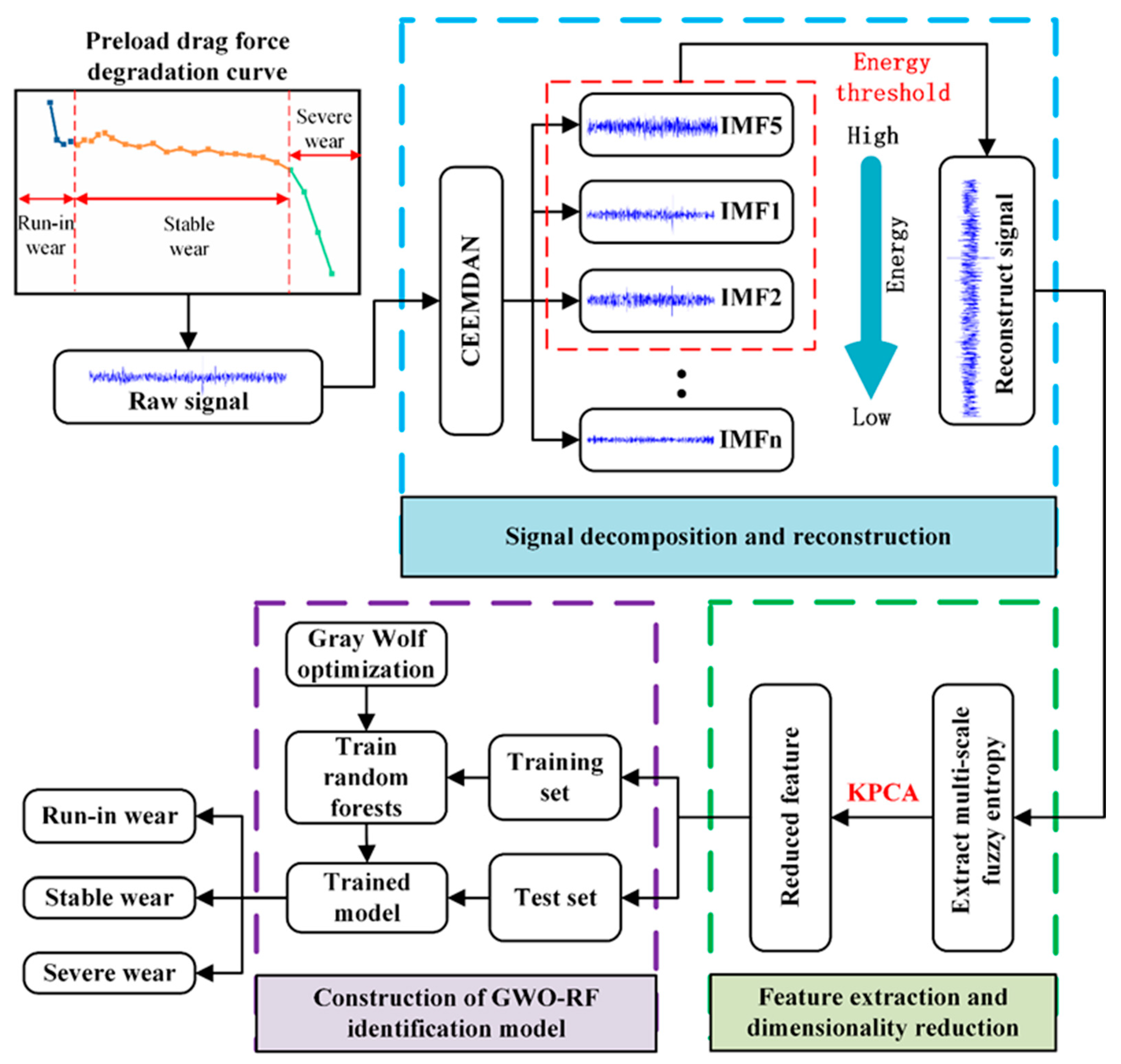
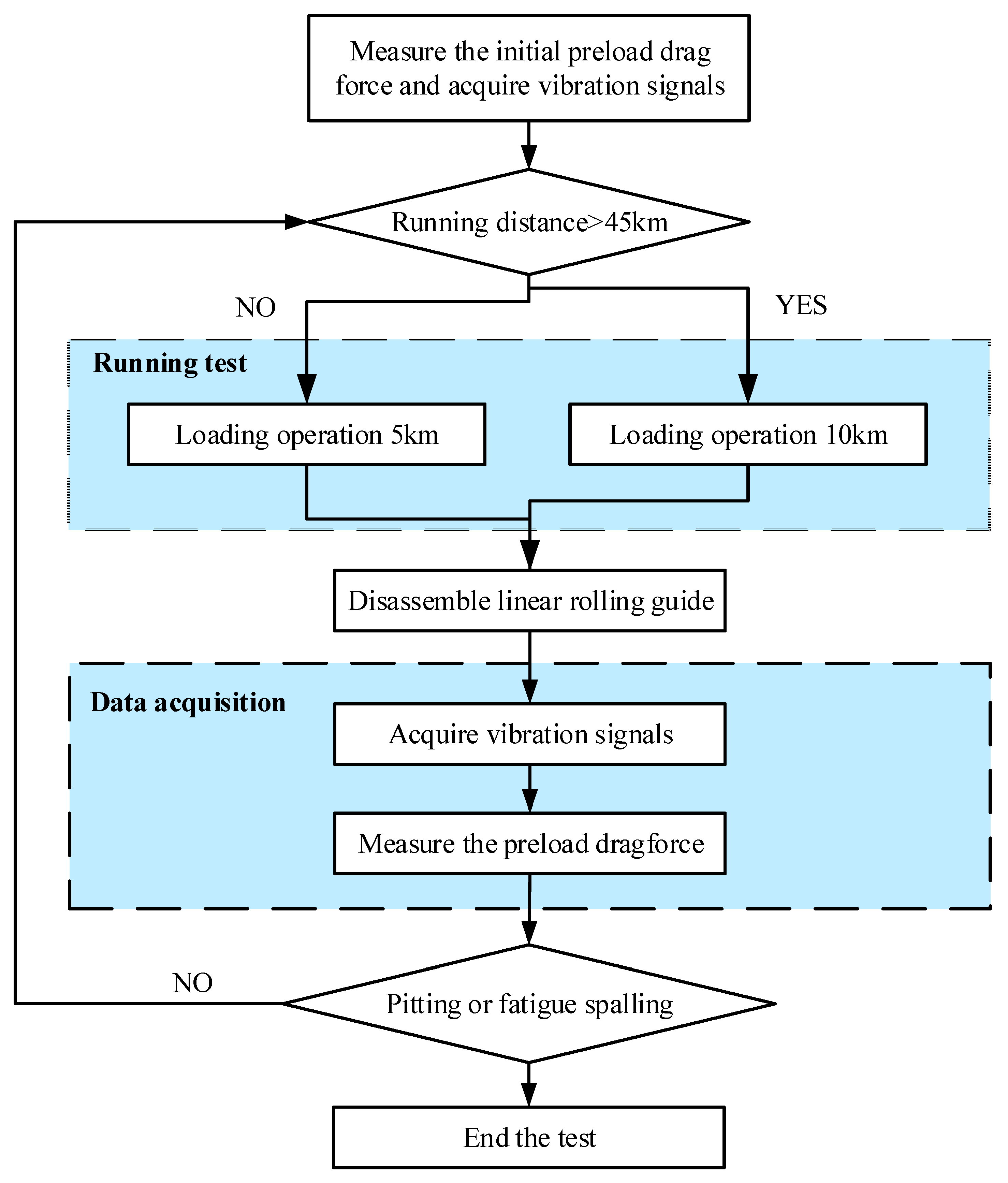
To accurately identify the surface wear state of LRGs, this study proposes a comprehensive method integrating signal processing, feature extraction, and machine learning. The overall process is illustrated in Figure 1, which can be divided into four key steps:

(1)

Signal acquisition and wear stage division: Full-period vibration signals during the LRG surface wear process were collected, and the wear process was divided into three stages (run-in wear, stable wear, and severe wear) based on the degradation trend of preload drag force.

(2)

Signal decomposition and reconstruction: The original vibration signals were decomposed using complete ensemble empirical mode decomposition with adaptive noise (CEEMDAN) to obtain multiple intrinsic mode function (IMF) components. IMFs meeting the energy threshold were selected for signal reconstruction to reduce noise interference.

(3)

Feature extraction and dimensionality reduction: Multi-scale fuzzy entropy (MFE) was extracted from the reconstructed signals to construct a feature set, and kernel principal component analysis (KPCA) was applied for dimensionality reduction to simplify the feature space.

(4)

Wear state classification: The reduced features were input into a gray wolf-optimized random forest (GWO-RF) model for training and prediction, achieving accurate identification of wear states.

2.1. Decomposition and Reconstruction of CEEMDAN

Under normal circumstances, the acquired vibrational signal from an LRG has a high noise content and a low signal-to-noise ratio, which increases the difficulty of characterizing performance degradation. Therefore, it was necessary to apply noise reduction to the acquired signal. Empirical mode decomposition (EMD) has been extensively applied to nonlinear and non-stationary signals owing to its non-parametric characteristics and decomposition capability. However, EMD suffers from modal aliasing and endpoint effects and may produce spurious components that do not exist in the original signal [21]. Ensemble empirical mode decomposition (EEMD) reduces modal aliasing and extreme point effects by superimposing white noise onto the original signal to generate a new signal for decomposition. However, EEMD fails to fully suppress residual auxiliary noise, and the Gaussian white noise added in each decomposition varies randomly. As a result, it cannot ensure that the number of intrinsic mode function (IMF) components remains consistent across decompositions [22]. Adaptive noise-based CEEMDAN is employed to derive the first IMF component and the first remainder by performing EMD on the original signal superimposed with Gaussian white noise. The first remainder is then superimposed with noise for subsequent EMD decomposition. This iterative process allows the method to resolve the limitations of EMD and EEMD decomposition until the termination criterion is met [23]. The CEEMDAN decomposition procedure is outlined as follows:

(1)

Gaussian white noise is superimposed on the original signal to generate the decomposed signal:

$$x_i\left(t\right)=x\left(t\right)+n_i$$

(1)

The average of the first IMF component is calculated. The component was obtained through the EMD decomposition of $x_i\left(t\right)$, based on which the first-order modal component of the CEEMDAN decomposition:

$$\overline{IM{F}_1}={\displaystyle \frac{1}{n}}\sum _{i=1}^{n}IM{F}_{1i}$$

(2)

(2)

The first-order modal component residuals $r_1\left(t\right)$ are calculated as follows:

$$r_1\left(t\right)=x\left(t\right)-\overline{IM{F}_1}$$

(3)

(3)

White noise is added to the remainder of the modal component obtained in Equation (2) to construct a new decomposed signal of $r_1\left(t\right)+{\epsilon }_1{E}_1\left(n_i\right)$, and the second modal component $\overline{IM{F}_2}$ can be obtained as follows:

$$\overline{IM{F}_2}={\displaystyle \frac{1}{n}}\sum _{i=1}^n{E}_1\left(r_1\right(t)+{\epsilon }_1{E}_1(n_i\left)\right)$$

(4)

(4)

The second-order modal component residuals $r_2\left(t\right)$ are calculated as follows:

$$r_2\left(t\right)=r_1\left(t\right)-\overline{IM{F}_2}$$

(5)

(5)

Steps (1–4) were repeated until the extreme points of the margin signals were <3 to end the decomposition. Then, the K-order modal components and residuals were obtained, and the final decomposition result could be expressed as follows:

$$x(t)=\sum _{K=1}^K\overline{IM{F}_K}+r_K(t)$$

(6)

The extracted IMF components represented signal characteristics across distinct frequency bands, with those containing key information exhibiting higher amplitudes and correspondingly greater energy. Accordingly, all IMF components were arranged in descending order based on their energy contributions. IMF components with higher energy ratios indicated a greater influence on the original signal. The energy ratio of each IMF component was calculated as follows:

$$\left\{\begin{array}{c}{E}_i={\displaystyle \sum _{j=1}^N}x(j{)}^2\\ {\beta }_i={\displaystyle \frac{E_i}{\sum _{i=1}^M{E}_i}}\end{array}\right.$$

(7)

Here, $x\left(j\right)$is the corresponding amplitude of each point in the time series, N is the length of the time series, $E_i$is the energy of $IM{F}_i$, M is the number of IMFs obtained by decomposition, and ${\beta }_i$ is the energy proportion of the IMF component. The energy threshold was established after determining the energy ratio of each component. When the sum of the energy ratios of the current $k$-order IMF exceeded the set threshold, the previous $k$-order IMF was selected to reconstruct the signal. At this time, the reconstructed signal was considered to contain important information from the initial signal.

2.2. Feature Extraction and Dimensionality Reduction

2.2.1. Multi-Scale Fuzzy Entropy (MFE)

Fuzzy entropy [24] was used to measure the probability of generating a new pattern when the dimensionality of a time series varied. The complexity of the sequence increased with the entropy. For a $N$-point time series $\left\{u\right(i):1\le i\le N\}$, the vector $X_i^m$ is expressed as follows:

$$X_i^m=\left\{u\right(i),u(i+1)......u(i+m-1\left)\right\}-u0\left(i\right)$$

(8)

where $u0\left(i\right)$ is the mean value of the time series of length $m$, expressed as follows:

$$u0(i)={\displaystyle \frac{1}{m}}\sum _{j=0}^{m-1}u(i+j)$$

(9)

The distance between vector $X_i^m$and vector $X_j^m$is expressed by the maximum value of the difference between the corresponding elements of two vectors, i.e.:

$$d_{ij}^m=d\left[X_i^m,X_j^m\right]=\underset{k\in \left(0,m-1\right)}{max}\left|\left(u\right(i+k)-u0(i\left)\right)-\left(u\right(j+k)-u0(j\left)\right)\right|$$

(10)

The similarity between the vectors $X_i^m$ and $X_j^m$ is calculated by the fuzzy function$\mu (d_{ij}^m,n,r)$, which is in exponential form, i.e.:

$$D_{ij}^m(n,r)=\mu (d_{ij}^m,n,r)=\mathit{exp}(-(d_{ij}^m{)}^n/r)$$

(11)

where n and r represent the gradient and boundary width of the function, respectively.

The function ${\varphi }^m(n,r)$ was defined as follows:

$${\varphi }^m(n,r)={\displaystyle \frac{1}{N-m}}\sum _{i=1}^{N-m}({\displaystyle \frac{1}{N-m-1}}\sum _{j=1,j\ne i}^{N-m}{D}_{ij}^m)$$

(12)

Similarly, the above steps for the vector $X_i^{m+1}$ were repeated to obtain the function ${\varphi }^{m+1}(n,r)$.

$${\varphi }^{m+1}(n,r)={\displaystyle \frac{1}{N-m}}\sum _{i=1}^{N-m}({\displaystyle \frac{1}{N-m-1}}\sum _{j=1,j\ne i}^{N-m}{D}_{ij}^{m+1})$$

(13)

Based on functions ${\varphi }^m(n,r)$ and ${\varphi }^{m+1}(n,r)$, the fuzzy entropy of the time series can be expressed as follows:

$$FuzzyEn(m,n,r,N)=\mathit{ln}({\varphi }^m(n,r)-\mathit{ln}({\varphi }^{m+1}(n,r))$$

(14)

MFE [25] introduces a scale factor ($\tau =\mathrm{1,2},.....$) to establish a new coarse-grained vector $\{x_1,x_2,......,x_N\}$ for the original sequence of length$N$.

$$y_j(\tau )={\displaystyle \frac{1}{\tau }}\sum _{i=(j-1)\tau +1}^{j\tau }{x}_i,1\le j\le {\displaystyle \frac{N}{\tau }}$$

(15)

When $\tau =1$, $y_j\left(1\right)$ is the original sequence. For $\tau >1$, the original sequence was split into coarse-grained vector sequences $y_j\left(\tau \right)$ of length $N/\tau$ at different scales. Then, the fuzzy entropy of the coarse-grained vector at each scale was calculated and expressed as a function of the scale factor.

The MFE analysis characterized the complexity and self-similarity properties of time series across multiple scale factors, consistent with the physical interpretation of fuzzy entropy at a single scale. If the entropy of one time series exceeded that of another across most scales, it was considered to exhibit greater complexity. Conversely, a decreasing trend of entropy with increasing scale factors indicated that the sequence possessed a relatively simple structure with richer information content at smaller scales.

2.2.2. Kernel Principal Component Analysis (KPCA)

The features reflecting the surface wear process of the LRG were extracted from the computed multi-scale fuzzy entropy (MFE) of the vibrational signals. However, when the dimensionality of the original feature space was excessively high, issues such as data sparsity and computational difficulties in distance measurement arose—commonly referred to as the “dimension disaster”. To address this dimensionality problem, it was essential to transform the original high-dimensional feature space into a lower-dimensional subspace through mathematical dimensionality reduction techniques. Given the complexity and variability of the LRG vibrational signals, the resulting feature space often exhibited nonlinear characteristics, necessitating the application of nonlinear dimensionality reduction methods. Kernel principal component analysis (KPCA) addressed this by mapping the original data to a higher-dimensional feature space via nonlinear transformation, followed by linear dimensionality reduction in that space. This approach enabled effective preservation of the original data structure while maximizing the extraction of underlying nonlinear information.

KPCA first normalized the initial data to obtain a new sample set $x_i(i=\mathrm{1,2},......,n)$, and then introduced a nonlinear function $\varphi \left(x\right)$ to map the sample set to the high-dimensional feature space F. The covariance matrix W can be expressed as follows:

$$W={\displaystyle \frac{1}{n}}\sum _{i=1}^n\varphi \left(x_i\right)\varphi (x_i{)}^T$$

(16)

The eigenvalues $\lambda$and eigenvectors A of the matrix W satisfy the following:

$$\lambda A=WA$$

(17)

A nonlinear function $\varphi (x_i{)}^T$ was introduced at both ends of Equation (17), and the eigenvector $A={\sum }_{j=1}^n{\alpha }_j\varphi \left(x_j\right)$ was substituted into Equation (17) to obtain:

$$\lambda \sum _{j=1}^n{\alpha }_j\varphi (x_i{)}^T\varphi (x_j)=W\sum _{j=1}^n{\alpha }_j\varphi (x_i{)}^T\varphi (x_j)$$

(18)

Combining Equation (16) with Equation (18) results in:

$$\lambda \sum _{j=1}^n{\alpha }_j\varphi (x_i{)}^T\varphi (x_j)={\displaystyle \frac{1}{n}}\sum _{i=1}^n\varphi (x_i)\varphi (x_i{)}^T\sum _{j=1}^n{\alpha }_j\varphi (x_i{)}^T\varphi (x_j)$$

(19)

In general, the form of the mapping function $\varphi$was unknown; thus, the kernel function $\kappa$ was introduced:

$$\kappa (x_i,x_j)=\varphi \left(x_i{)}^T\varphi \right(x_j)$$

(20)

Equation (19) could be expressed as follows:

$$KA=n\lambda A$$

(21)

where K is the $\kappa$corresponding kernel matrix, whose eigenvalue is $n\lambda$, and whose corresponding eigenvector is $A=({\alpha }_1;{\alpha }_2;......;{\alpha }_n)$. For any sample, the projection of the data in the high-dimensional feature space F on the feature vector $V_k(k=\mathrm{1,2},...,d)$ was the principal component feature of the initial data, expressed as follows:

$$V_{\varphi \left(x\right)}=\sum _{j=1}^n{\alpha }_j^k\varphi (x_j{)}^T\varphi (x)=\sum _{j=1}^n{\alpha }_j^k\kappa (x_j,x)$$

(22)

2.3. Random Forest-State Recognition Based on the Gray Wolf Optimization Algorithm (GWO-RF)

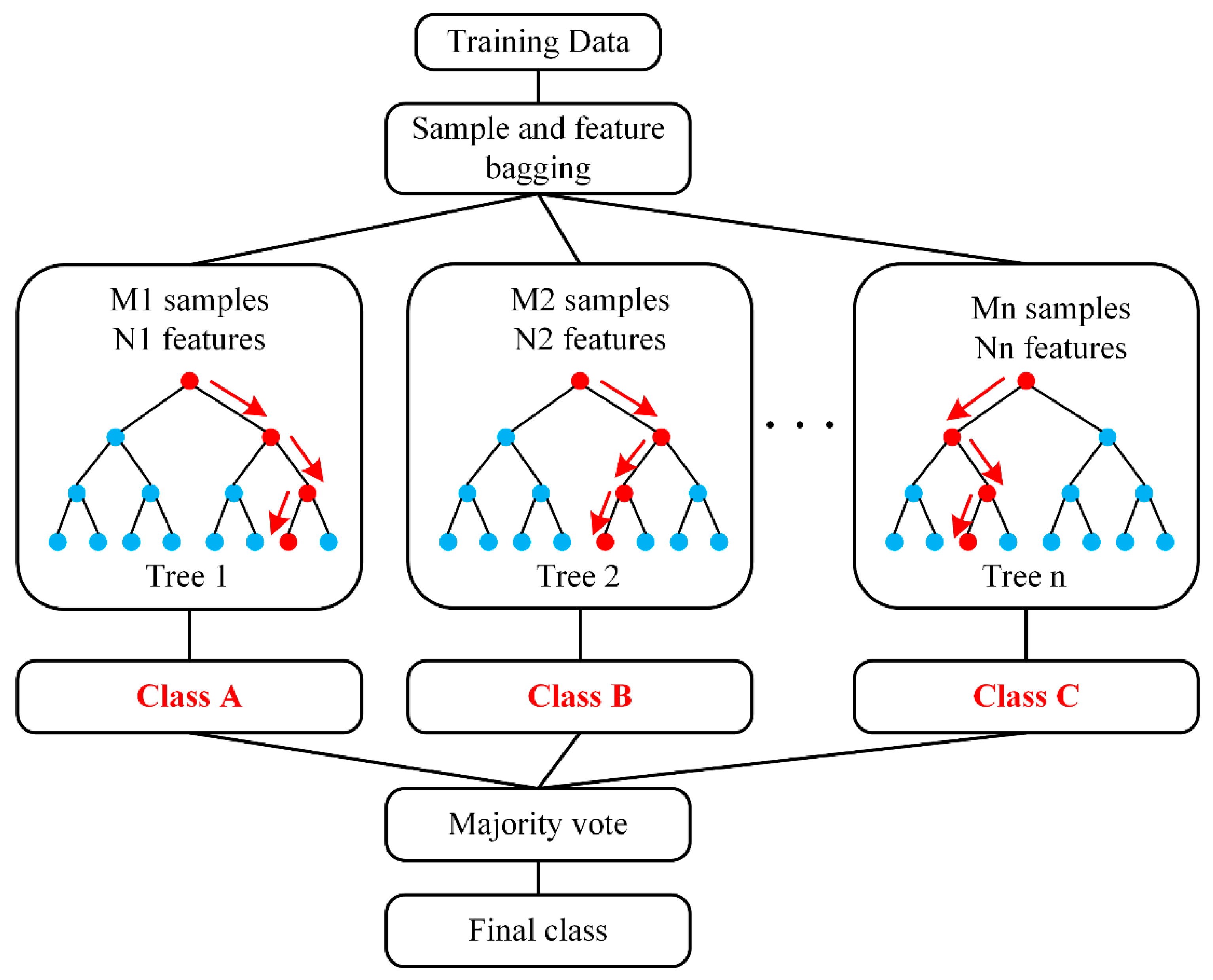
Ensemble learning is a machine-learning method that completes the classification task by constructing and combining multiple classifiers to improve prediction performance. Examples include boosting, bagging, and stacking, where bagging is parallel ensemble learning. For a collection of data sets containing m samples, we first randomly selected a sample and placed it in the sampling set. Then, it was put back in the initial data set so that it may be chosen again for subsequent sampling. The process was repeated $m$times to obtain a set containing $m$samples. In this way, T sample sets containing $m$training samples were obtained. Each sample set was used to train the base learner, which was blended using straightforward voting to create an ensemble learner. Random forest (RF) [26] is an extended variant of bagging, and its principle is depicted in Figure 2. Based on the decision-tree-based learner to build bagging, a random attribute selection was introduced in the training of the decision tree. The optimal attribute was selected from the attribute set of the current node (assuming there were $n$attributes) to separate the properties. RF randomly selected a subset of $k$attributes from the attribute set of each node of the base decision tree and then selected an optimal attribute from the subset for division. The degree of randomness introduced was determined by the parameters k, where $k={\mathit{log}}_{2}n$was usually selected. RF not only guaranteed randomness but also avoided over-fitting of the model by double sampling of samples and features.

The choice of some hyperparameters in the RF algorithm affected the classification performance and robustness of the model. To improve the performance of the trained model, it was necessary to optimize the hyperparameters. The gray wolf optimization algorithm (GWO) is a swarm-intelligence optimization algorithm, which was derived from simulating the hierarchical mechanism and hunting behavior of actual gray wolves in nature. Assuming that the wolf pack social structure comprised wolf $\alpha$, wolf $\beta$, wolf $\delta$, and wolf $\omega$ from high to low, their predation behavior during hunting could be expressed as follows:

$$D=\left|C\cdot X_P^t-X^t\right|$$

(23)

$$X^{t+1}=X_P^t-A\cdot D$$

(24)

where D represents the distance between an individual gray wolf and the prey, $X_P^t$represents the prey position vector, $X^t$represents the current position of the gray wolf, and t is the number of iterations. The next position of the gray wolf was determined by Equation (24). A is the convergence factor and C is the swing factor, expressed as follows:

$$\left\{\begin{array}{c}A=2a{r}_1-a\\ C=2r_2\end{array}\right.$$

(25)

where $r_1$ and $r_2$ are random numbers between 0 and 1. $a$ is the distance control parameter, which decreased linearly from 2 to 0 as the number of iterations increased. Assuming that $\alpha$, $\beta$, and $\delta$ had a stronger ability to identify the potential position of the prey, the positions of the three wolves were retained during each iteration and used to judge the position of the prey. At the same time, other gray wolves updated their positions in accordance with that of the optimal gray wolf. The final position of the gray wolf attacking the prey can be described as follows:

$$X^{t+1}={\displaystyle \frac{X_1+X_2+X_3}{3}}$$

(26)

where $X_1{X}_2{X}_3$ are the updated positions of $\alpha$, $\beta$, and $\delta$, respectively, based on their distance from other gray wolves.

Here, the RF was built based on the GWO method, by optimizing the number of decision trees with a minimal number of leaf nodes. In general, higher numbers of decision trees yielded better model effects. However, the accuracy of the model fluctuated when the quantity reached a certain point. Meanwhile, the required calculations and memory increased, and the training time increased. The minimum number of leaf nodes mainly controlled the minimum number of leaf node samples. If the number of leaf node samples was less than the parameter value, it no longer branched.

3. Experiments and Method Verification

The experimental data utilized in this study were obtained from full-cycle vibrational signals of the LRG. The SHS35R series linear guide, manufactured by THK Co., Ltd. (Tokyo, Japan), was selected as the test specimen. The nominal basic static load rating (C₀) of the specimen was 96.6 kN, while its basic dynamic load rating (C) was 62.3 kN. The experimental setup comprised a running test platform, a preload drag-force measurement platform, and a vibration data acquisition system. All experiments were conducted in a constant-temperature laboratory equipped with a dehumidifier, maintaining the ambient temperature within 20 ± 2 °C and relative humidity ≤ 80%. Additionally, during the acquisition of vibration and preload drag-force signals, all other large-scale equipment in the laboratory was shut down to eliminate external noise interference.

3.1. Running Test Bench

The running test was conducted on the dedicated test platform (Figure 3) to obtain performance parameters characterizing the surface wear state of the LRG. The test platform was composed of a bed frame, a gantry loading mechanism, a servo motor (①), a rack-and-pinion transmission system (②③), a guide rail adapter plate (⑧), and two linear guide pairs (⑦) [27]. The LRG under test was mounted on the adapter plate, with a cushion block (④) installed on the carriage. The load was applied to the carriage via hand wheels (⑥) positioned on both sides of the gantry loading mechanism. A FN3000-A2 force sensor (⑤) (Supply Voltage, Sensitivity “FSO”2:) installed on the loading block measured the applied load and transmitted the data to the acquisition system. The reciprocating motion of the carriage was realized by the servo motor driving the rack-and-pinion mechanism. During testing, the applied load corresponded to 40% of the rated dynamic load, with a running speed of 50 m/min and a unidirectional travel distance of 1100 mm.

3.2. Preload Drag-Force Test Bench

The preload drag-force LRG performance indicator deteriorated because of surface wear between the rolling elements and the raceway. The schematic of the preload drag-force test system is shown in Figure 4, consisting of a bed frame, a servo motor, a workbench, a dynamometer, and a computer. The dynamometer was securely installed on the workbench, which was driven by the servo motor to achieve the reciprocating motion of the carriage. The running speed of the carriage was 0.7 m/min, and the dynamometer sampled data at a rate of 100 Hz. The total measuring length, corresponding to the carriage’s travel distance, was 1100 mm. The preload drag force was measured three times during both forward and reverse strokes. To minimize the influence of acceleration and deceleration phases, only the data collected from the constant-speed segment (990 mm) were used to calculate the average preload drag force.

3.3. Vibrational Data Acquisition

A vibrational signal acquisition system was constructed, similar in configuration to the preload drag-force test platform, to capture vibration signals of the LRG under different surface wear conditions. As shown in Figure 5, vibration sensors were mounted on the top and side surfaces of the carriage, as well as on the top surface at the guide rail’s end. The sensitivities of the sensors were 501.33 mV/g, 488.97 mV/g, and 489.64 mV/g, respectively. The ProsigP8020 data acquisition system operated at a sampling frequency of 5000 Hz, corresponding to carriage speeds of 7 m/min, 14 m/min, and 21 m/min.

Figure 6 shows the LRG test procedure. First, the initial preload drag force (0.7 m/min) and vibrational signals (7 m/min, 14 m/min, 21 m/min) were recorded. Then, the LRG operated the running test bench under a vertical load of 40% C (24.92 kN) at 50 m/min. Measurements were taken every 5 km up to 45 km and every 10 km thereafter, continuing until fatigue spalling occurred on the carriage raceway.

4. Results and Discussion

4.1. Test Results

As shown in Figure 7a, the preload drag-force degradation of the LRG exhibited three distinct stages. From 0 to 20 km, the force dropped sharply, representing the run-in surface wear stage. Between 20 and 175 km, the decline slowed, indicating stable surface wear. From 175 to 205 km, the force again decreased rapidly, corresponding to severe surface wear. Figure 7b presents images of the carriage raceway surface at each stage, revealing large fatigue spalling after 205 km. 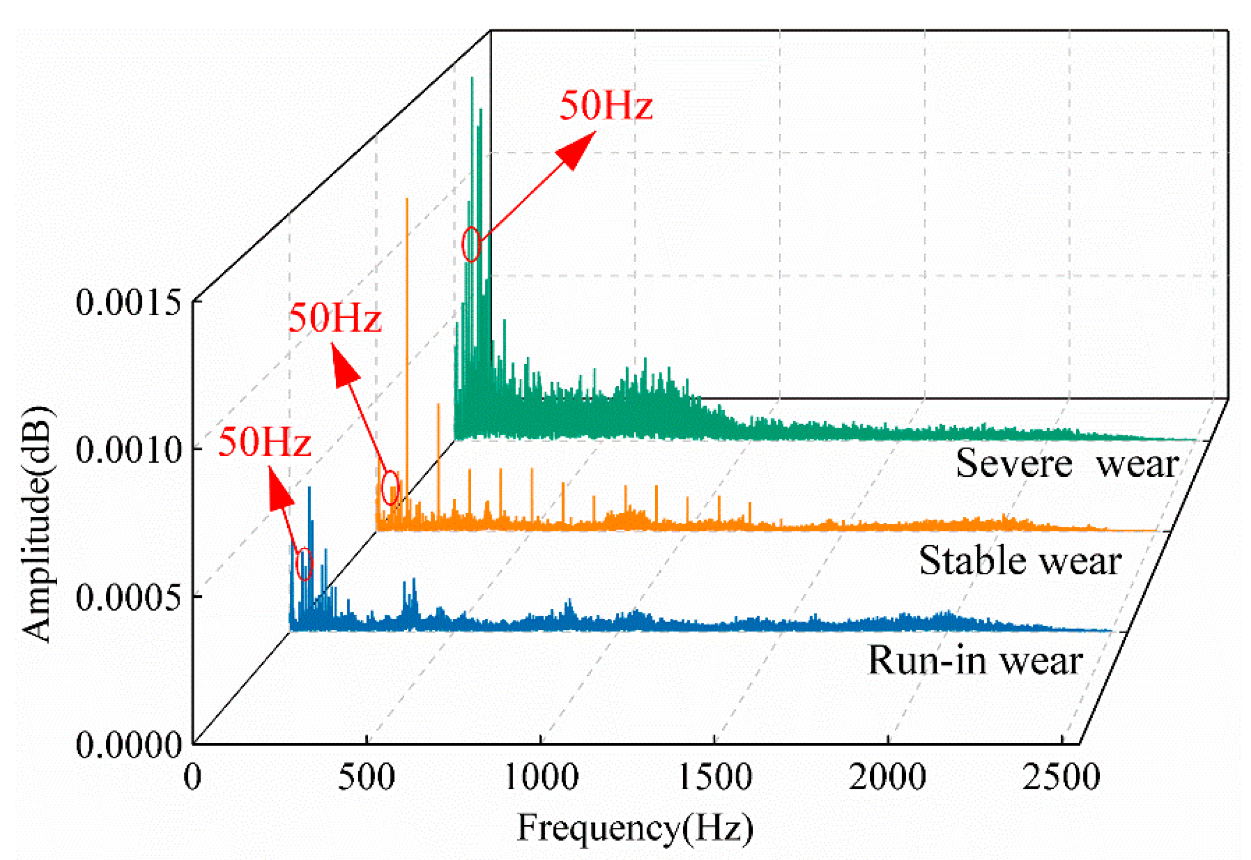Figure 7c shows the vibration signals over the full test period, with noticeable variation only during severe surface wear. As shown in Figure 8, there are distinguishable trends among different wear states in specific frequency bands (e.g., around 50 Hz and in the high-frequency range). However, we found that in terms of actual recognition performance, traditional frequency-domain features (such as spectral peaks and energy distribution) still exhibit lower discriminative power compared to MFE features. Therefore, further signal processing was necessary to extract meaningful surface wear-related features.

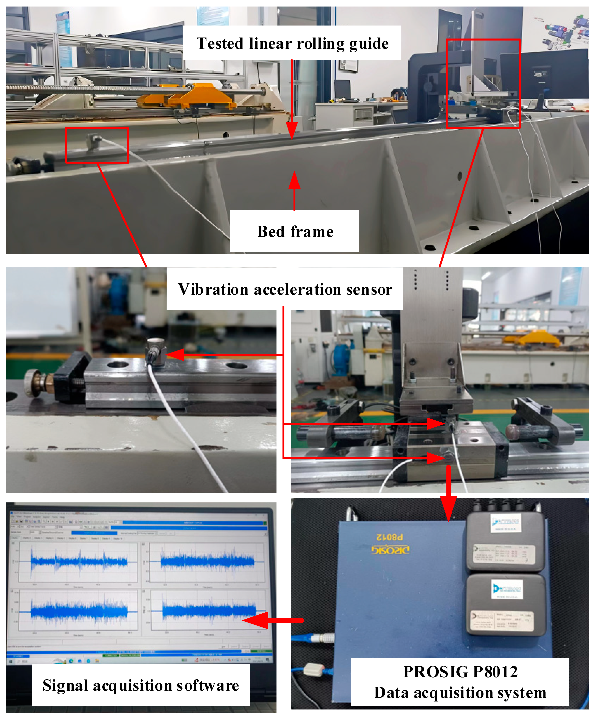
The vibration signal collected at 7 m/min from the top surface of the carriage was used to validate the method. The dataset comprised 100 samples for the run-in surface wear stage, 320 samples for the stable surface wear stage, and 60 samples for the severe surface wear stage. Each sample contained 1024 data points, forming the complete dataset ($480\times 1024$).

4.2. Results of Signal Decomposition and Reconstruction

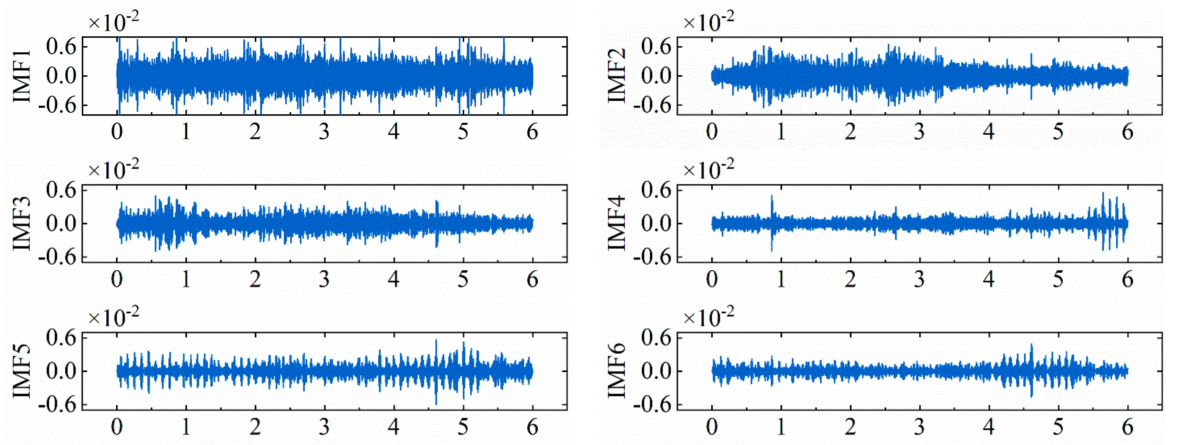
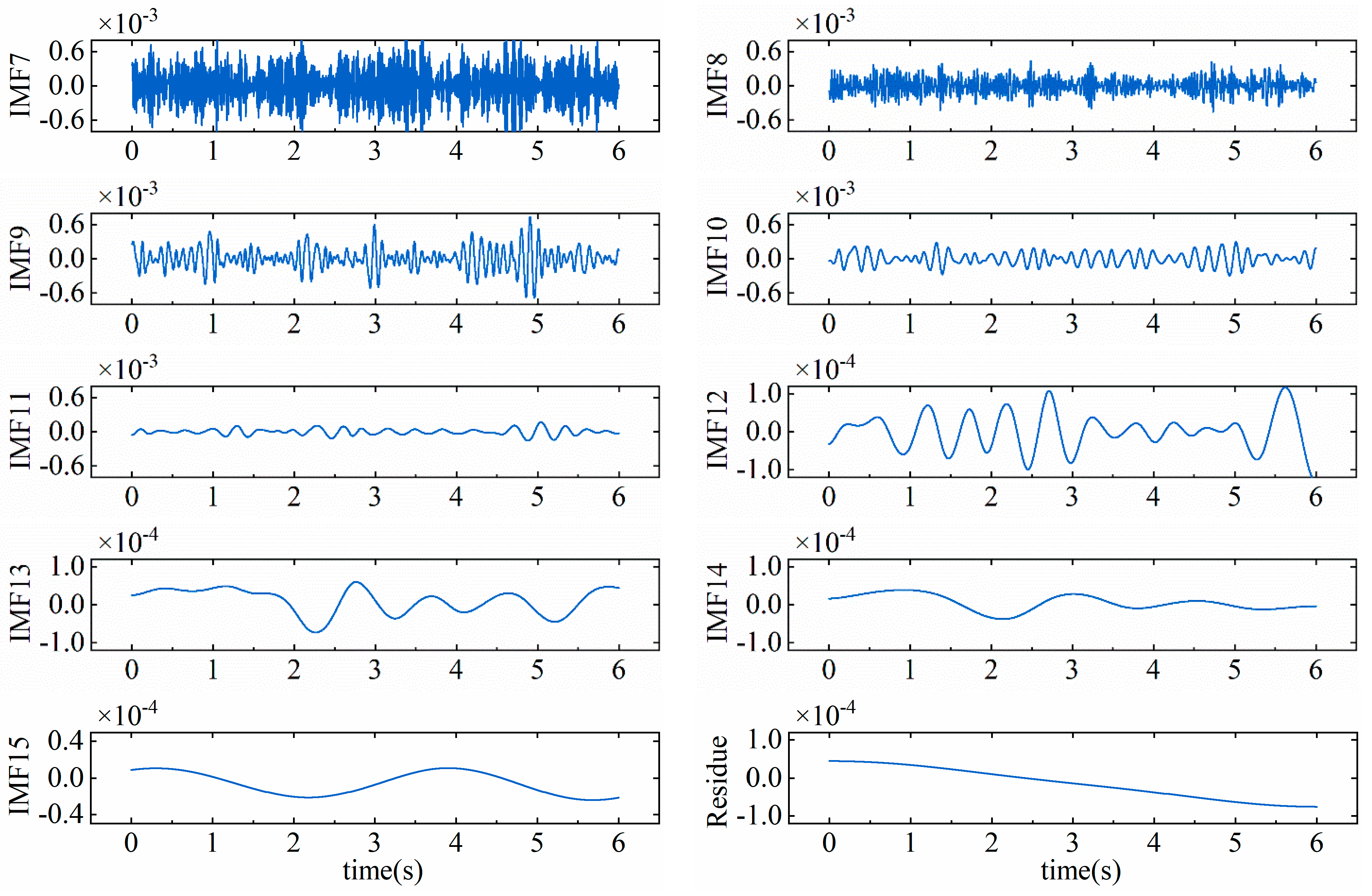
To enhance the accuracy of surface wear-state recognition, CEEMDAN decomposition was applied to denoise the initial signal before feature extraction. Gaussian noise with a standard deviation of 0.2 was added 100 times, with a maximum of 500 iterations. The resulting IMF and residual components from CEEMDAN decomposition are show in Figure 9. The IMF components, arranged from IMF1 to the residual, contained information corresponding to different frequency bands in descending order.

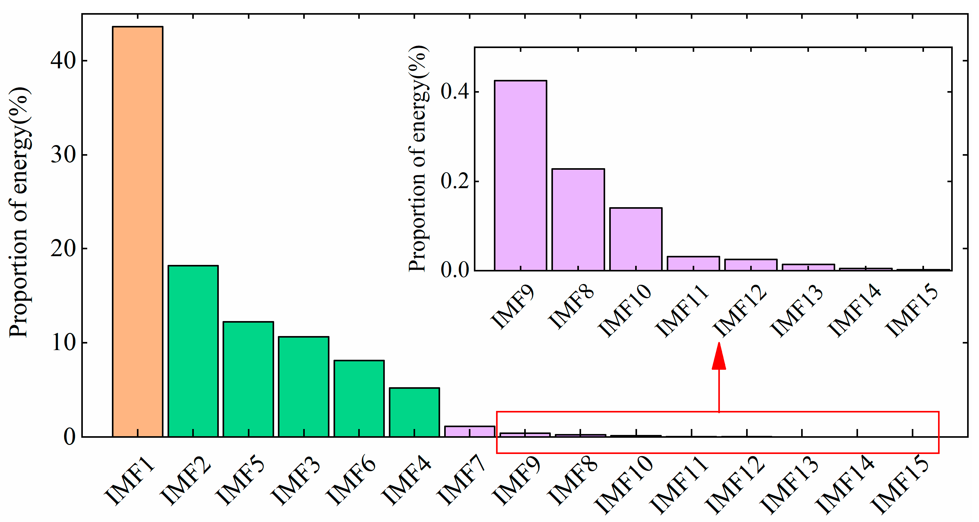
Figure 10 shows the energy proportions of the IMF components in descending order. A threshold of 70% was set for the total proportion. The top three components, IMF1, IMF2, and IMF5, contributed a combined energy proportion of 0.74047, exceeding the threshold. Therefore, these three components were selected to reconstruct the vibration signal.

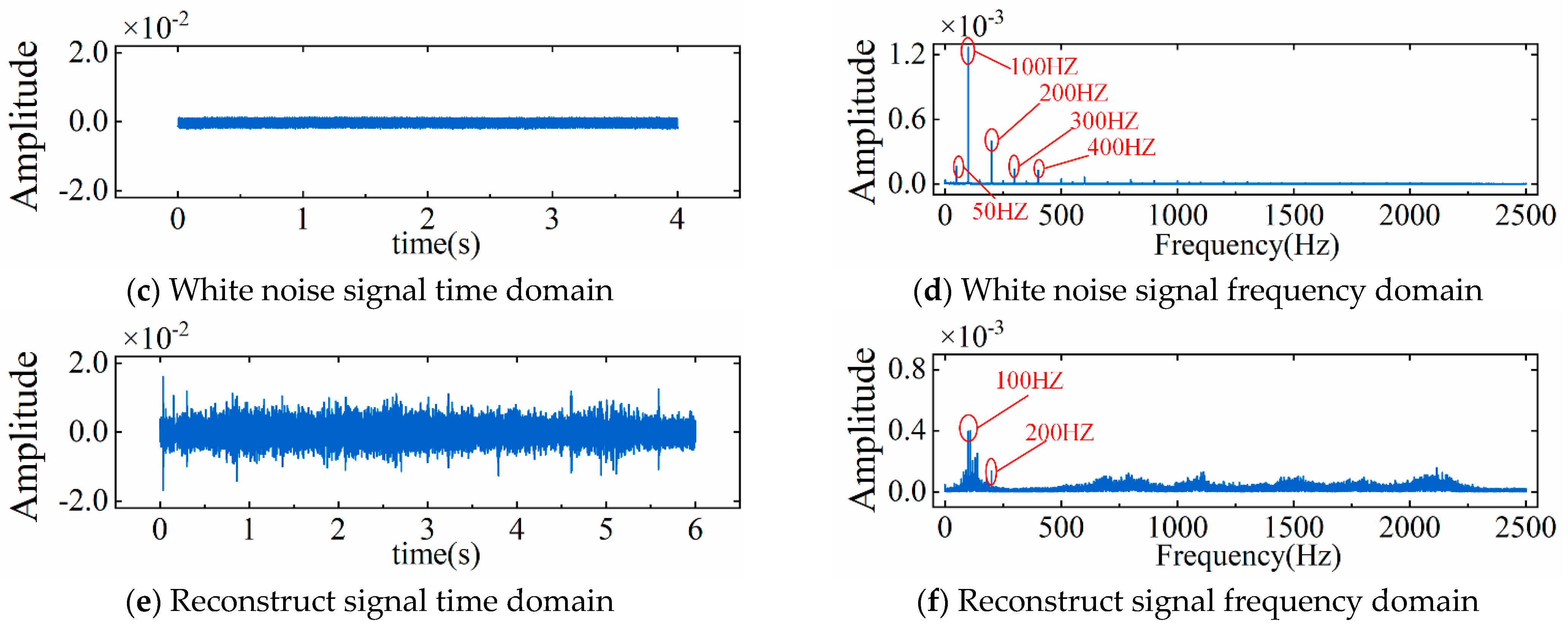
Figure 11 presents a comparison of the initial signal, the white-noise signal, and the reconstructed signal of the LRG in both time and frequency domains. The added white noise contained frequencies of 50 Hz, 100 Hz, 200 Hz, 300 Hz, and 400 Hz. After reconstruction, low-frequency noise within the 50–400 Hz range was effectively suppressed. This demonstrated the method’s capability for noise reduction and enhancement of the LRG vibration signal.

4.3. Results of Feature Extraction and Dimensionality Reduction

Feature extraction from the vibrational signal was crucial for identifying the surface wear condition of the LRG. The reconstructed signal was analyzed using MFE, which required five manually defined parameters: the embedding dimension m, the data length N, the similarity tolerance r, the fuzzy function gradient $n$, and the scale factor $\tau$ [27]. The relationship between the data length and the embedding dimension satisfied $N=10^m\sim 30^m$. Each data group contained 1024 points with m set to 3. The similarity tolerance was generally $0.1\sim 0.25SD$, and r = 0.15SD. The fuzzy function gradient n was generally two. The fuzzy entropy of the reconstructed signal was calculated at sixteen scales; therefore, $\tau =16$.

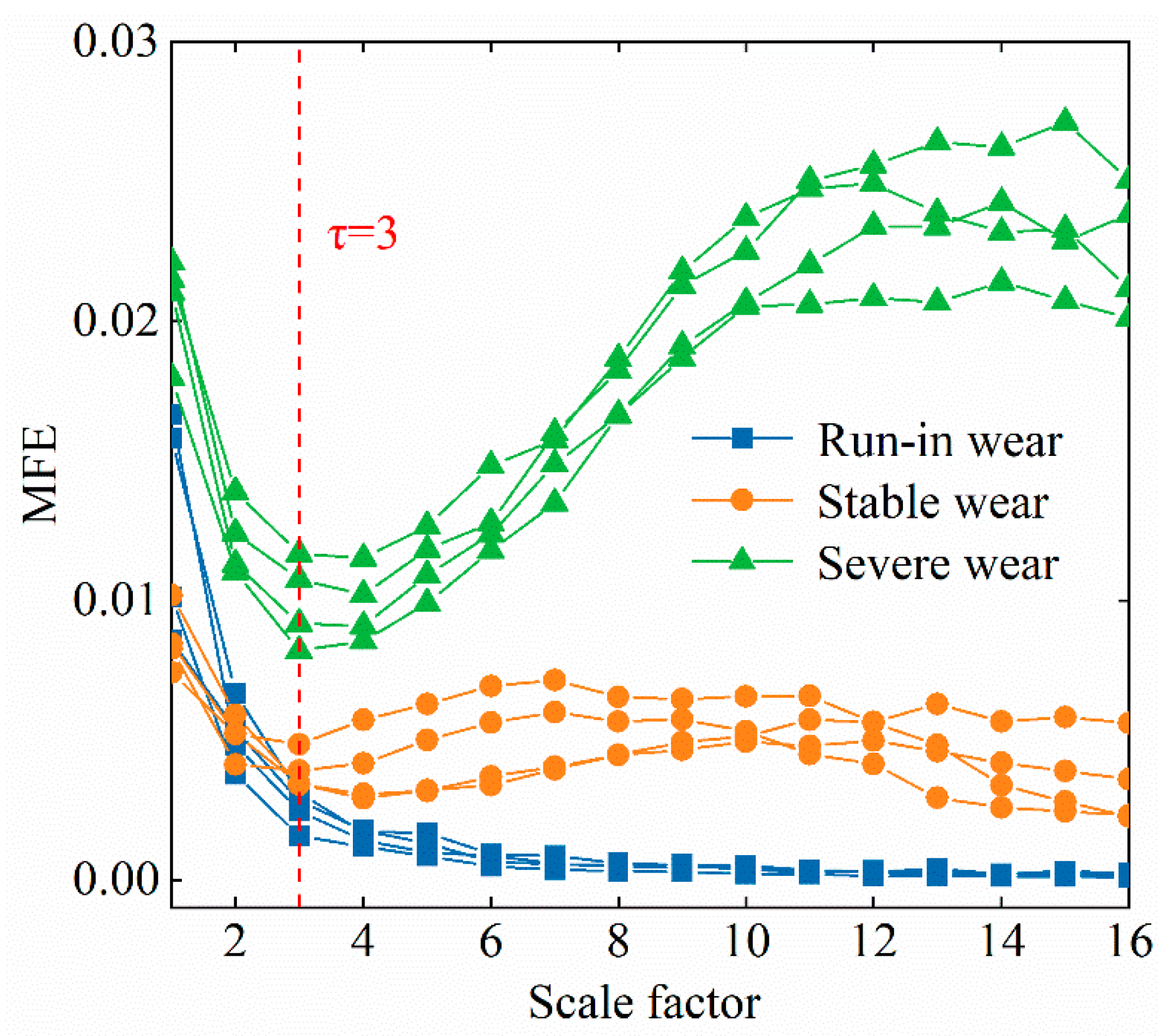
Figure 12 shows the MFEs obtained from vibrational signals corresponding to the three surface wear states. Four data sets were randomly selected for each state, and the signals were generally distinguishable. When the scale factor was less than 3, the entropy values ranked from high to low as severe surface wear, run-in surface wear, and stable surface wear. When the scale factor exceeded 3, the ranking shifted to severe surface wear, stable surface wear, and run-in surface wear. The entropy for the severe surface wear state first decreased, then increased, and eventually stabilized as the scale factor increased. The stable surface wear state exhibited a similar trend with smaller fluctuations. In contrast, the entropy of the run-in surface wear state rapidly decreased before stabilizing. Therefore, the fuzzy entropy at a single scale could not fully represent the surface wear condition, and multi-scale features were necessary to characterize the LRG surface wear state.

After obtaining the MFEs of the reconstructed signals, sixteen features were extracted from each data set. The initial sixteen-dimensional feature space was compressed to three dimensions using KPCA. The effectiveness of this dimensionality reduction is illustrated in Figure 13 by comparing the original feature distribution with that after reduction. The reduced feature space exhibited clearer separation between surface wear states, facilitating accurate surface wear-state identification and classification.

4.4. Results of GWO-RF Classification

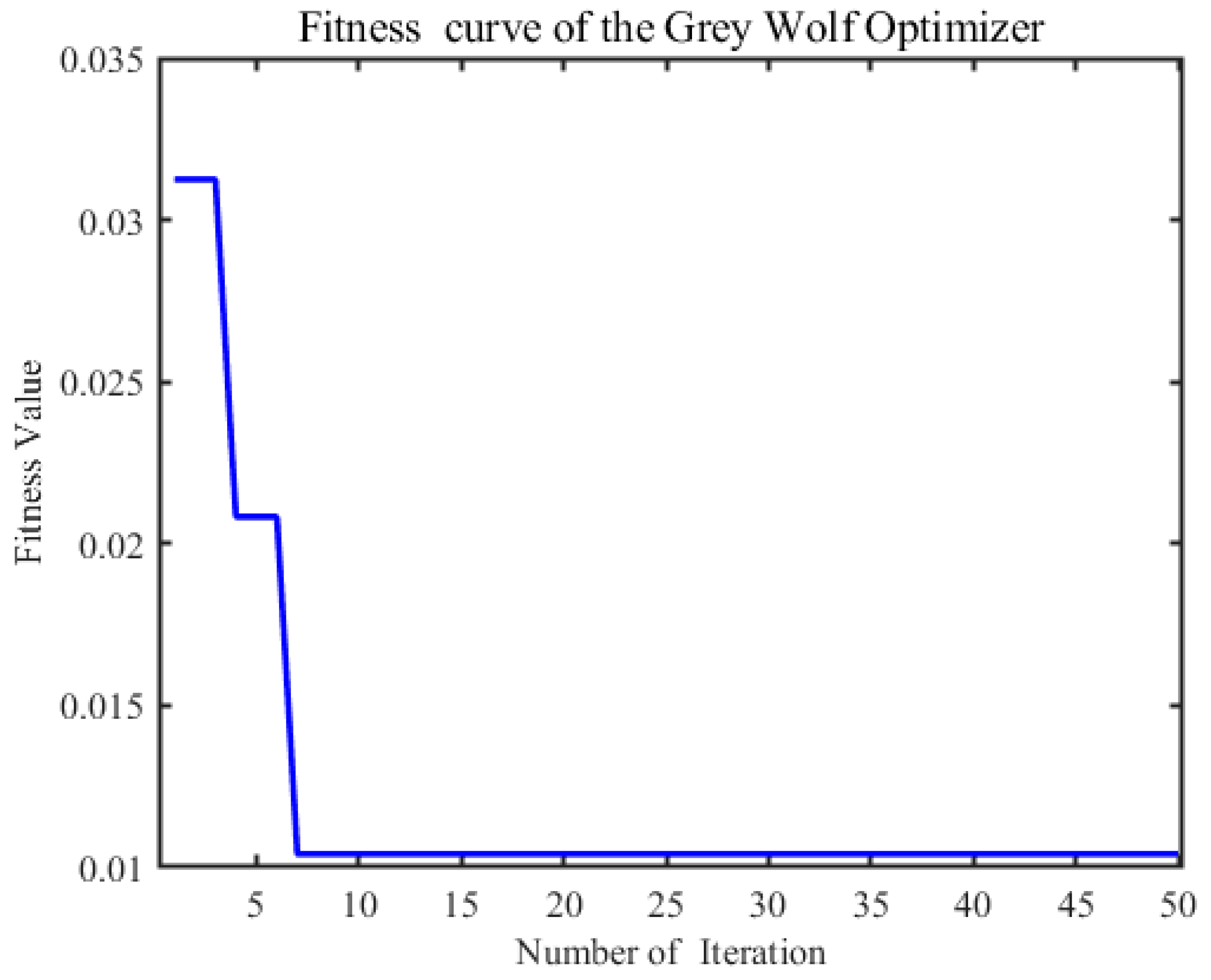
After decomposing and reconstructing the initial vibrational signals corresponding to the three surface wear states, MFE analysis and KPCA dimensionality reduction were applied to obtain a feature matrix. The data were divided into training and test sets at a ratio of 8:2, with 384 sets used for training and 96 sets for testing. Labels were assigned to the training data: 1 for run-in surface wear, 2 for stable surface wear, and 3 for severe surface wear. We optimized the hyperparameters involved in the Gray Wolf Optimizer (GWO), specifically the population size (10–20) and the number of iterations (1–50). The results indicate that a population size of 10 achieves the best fitness value while also minimizing the computation time. The corresponding results are shown in Figure 14. Thus, the random forest hyperparameters were optimized using the GWO algorithm with both the population size and the number of iterations set to 10.

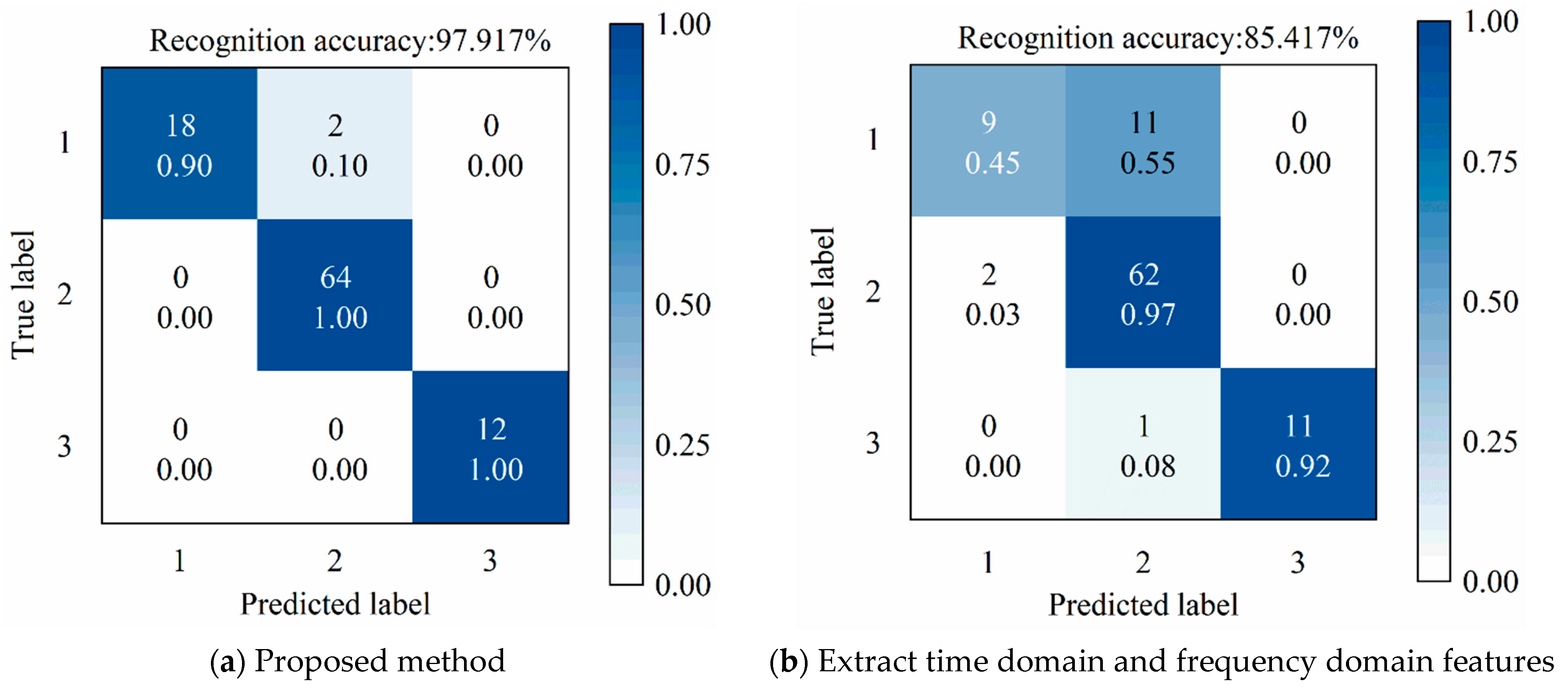
The optimized RF model employed 28 decision trees with a minimum of 4 leaf nodes. The trained model achieved a recognition accuracy of 97.9% on the test set, as shown in Figure 15a. Of the 96 test samples, 94 were correctly identified. To validate the statistical significance of the reported 97.9% accuracy, we calculated a 95% Wilson Score confidence interval of [92.7%, 99.4%] and performed a one-tailed hypothesis test (p < 0.001), both of which confirm that the model’s performance significantly exceeds random classification.

Two misclassifications occurred in the transition stage between running-in wear state and stable wear state. As shown in Figure 7a, the preload drag-force degradation curve of the linear rolling guide during the run-in test is divided into three stages. In the transition region between the run-in wear stage and the stable wear stage (around 20 km in the figure), the preload drag-force values fluctuate within a small range, indicating that the wear states of these two stages are extremely similar, and the corresponding vibration signals also have a high degree of similarity. This similarity in signal characteristics directly led to two misclassifications in this transition region. It should be emphasized that despite the above misclassifications, the wear degradation trend in this transition region has stabilized, so it will not significantly affect actual production and processing. Moreover, no misclassifications occurred in the stable wear stage and severe wear stage, which are crucial for actual machining. Therefore, the recognition results of this study still have important guiding significance for practical applications.

To evaluate the effectiveness of MFEs in surface wear-state recognition, conventional time-domain and frequency-domain features were also extracted from the reconstructed signals. These features, as reported in [28], were subjected to KPCA dimensionality reduction and surface wear-state identification using GWO-RF. The recognition accuracy, shown in Figure 15b, was 85.4%. Compared with conventional features, the MFE-based features significantly improved recognition performance, with an increase of 12.5% in accuracy. 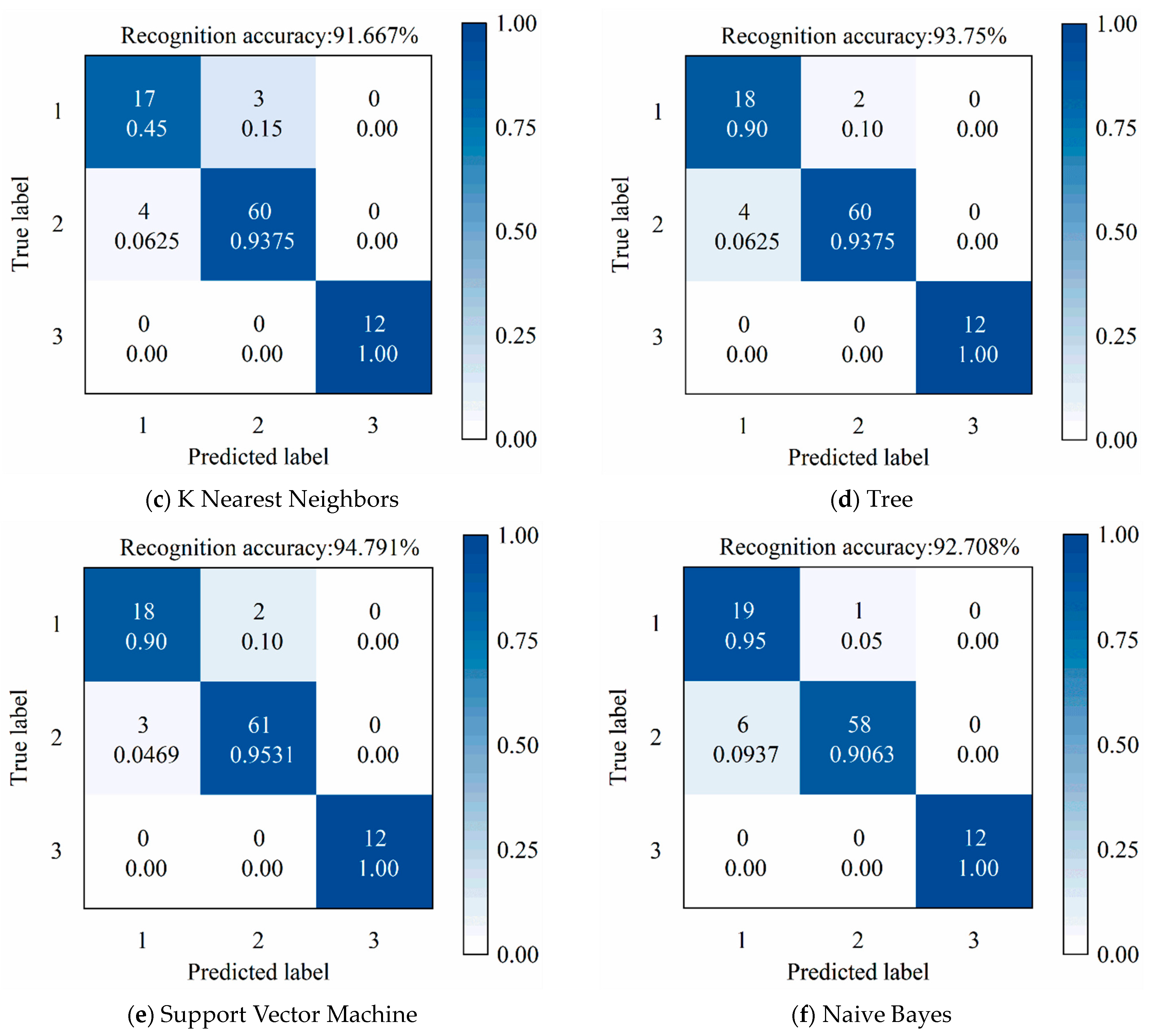Figure 15c–f further compares the recognition accuracy of different machine-learning algorithms. Among them, the GWO-RF method achieved the highest accuracy, confirming its superior performance in LRG surface wear-state recognition.

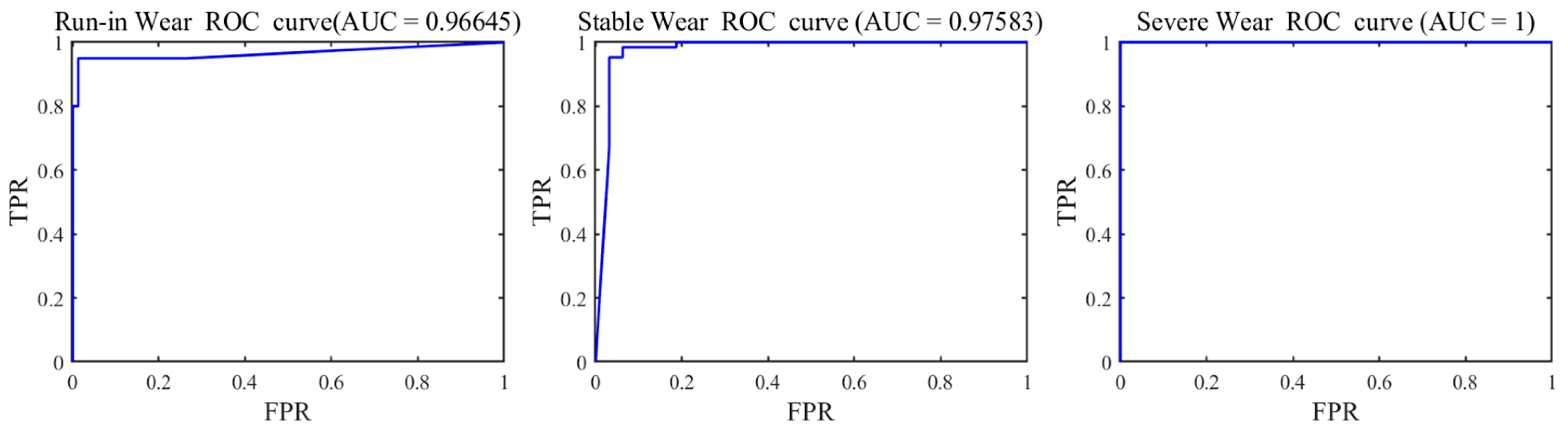
To further evaluate the classification performance of the model, a one vs. rest strategy was adopted to plot the ROC curves for each wear state (run-in wear, stable wear, and severe wear). As shown in Figure 16, the receiver operating characteristic (ROC) curves for all categories are close to the upper-left corner, and the areas under the curves (AUCs) are close to 1, indicating that the proposed method demonstrates excellent discriminative ability across all wear conditions.

Furthermore, the precision, recall, and F1-score for each category are summarized in

Table 1. Classification performance metrics for each wear state.

Category	Precision	Recall	F1 Score
Run-in wear	1	0.9	0.9474
Stable wear	0.9697	1	0.9846
Severe wear	1	1	1

.

In summary, these metrics collectively indicate that the proposed method in this paper has strong discriminative ability for the three wear states, with an overall excellent recognition effect.

4.5. Classification Results for Vibrational Signals at Various Positions and Speeds

Figure 17 presents the recognition results at different sensor positions and operating speeds, with the corresponding hyperparameters listed in

Table 2. Hyperparameters and recognition accuracies at various positions and speeds.

Speed (m/min)	Position	Number of Decision Trees	Minimum Number of Leaf Nodes	Recognition Accuracy (%)
7	Top surface	189	2	97.9
7	Side	70	3	88.5
7	Guide	89	4	92.7
14	Top surface	80	2	85.4
14	Side	98	6	92.7
14	Guide	39	2	96.9
21	Top surface	132	9	86.5
21	Side	101	4	91.7
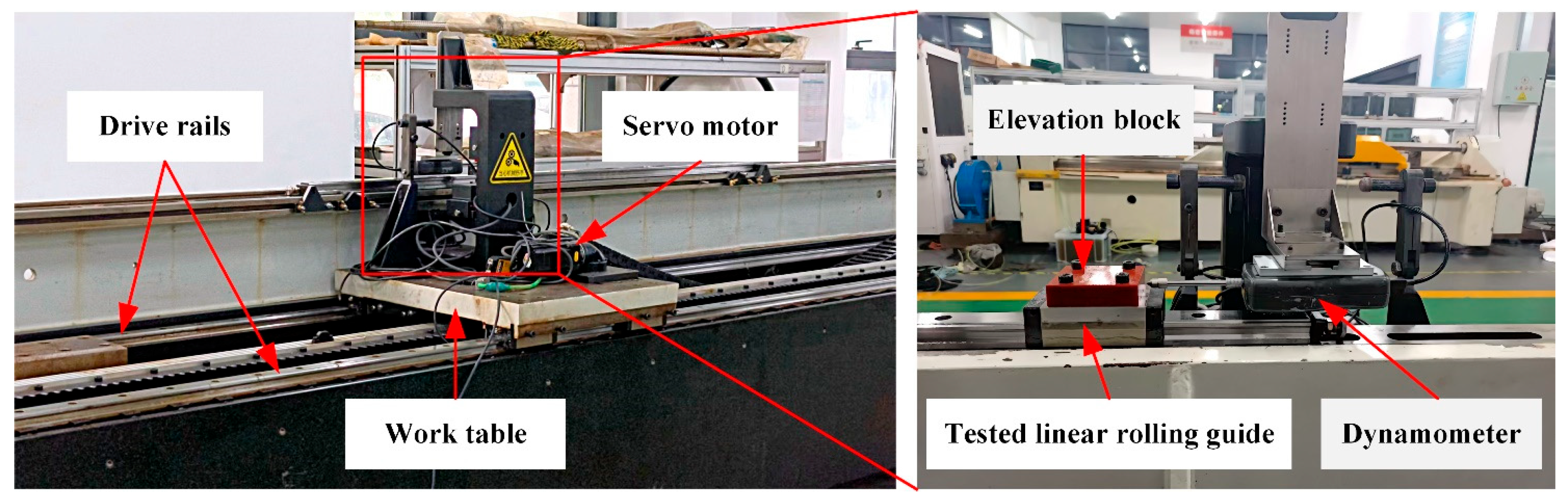
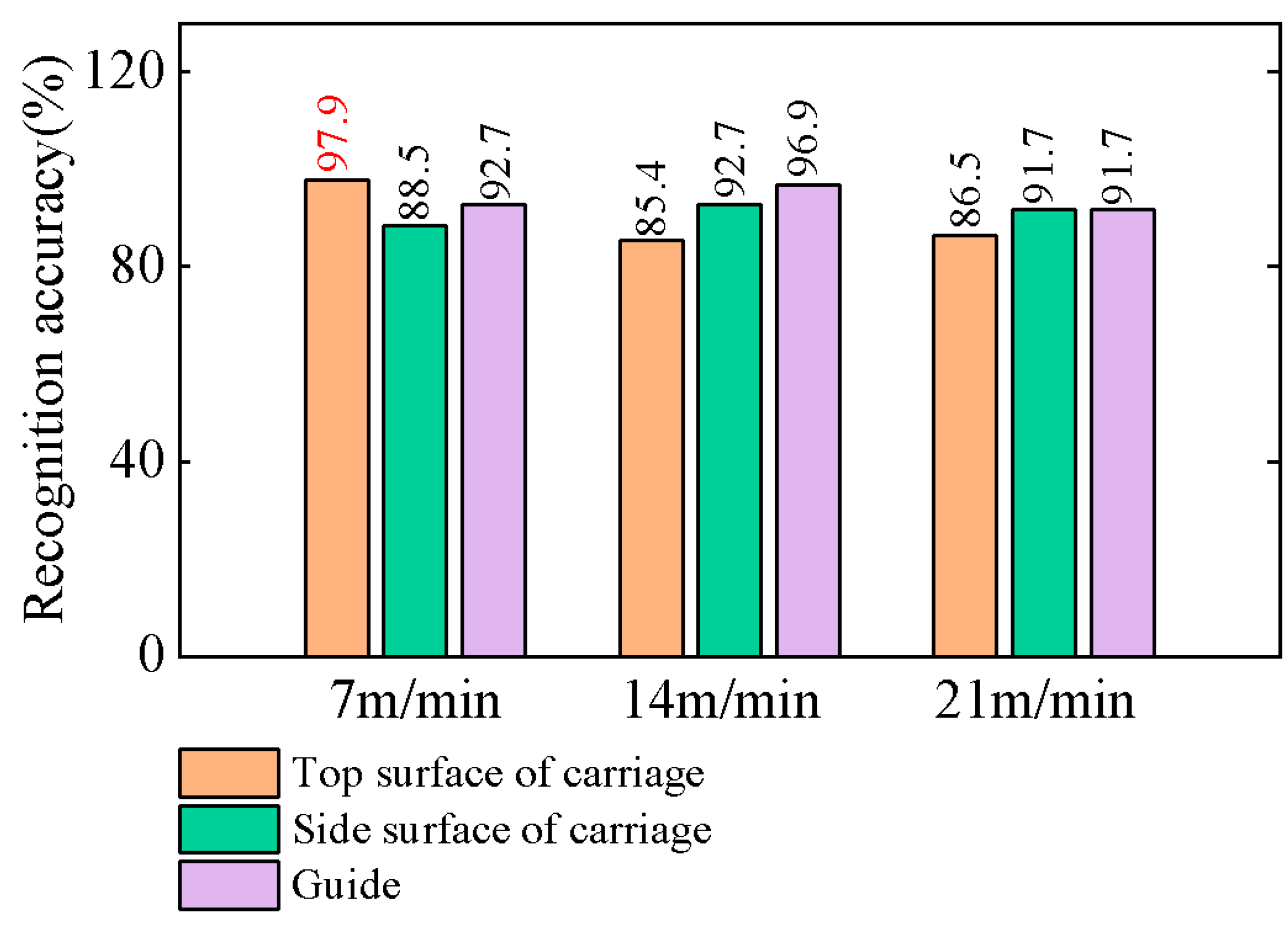
21	Guide	93	2	91.7

. The highest recognition accuracy was achieved by the vibration signal collected from the top surface of the carriage at 7 m/min, while lower accuracies were observed at 14 m/min and 21 m/min. For the signals collected from the side surface of the carriage, the recognition accuracies at the three speeds were all approximately 90%. In contrast, the signals acquired from the guide exhibited accuracies exceeding 90%, with the highest accuracy of 96.9% achieved at 14 m/min. Variations in carriage speed altered the rolling element frequencies within the return tube, and sensor positions resulted in exposure to different vibrational forces, leading to discrepancies in the acquired signals and recognition accuracy. These results confirm that the proposed method can effectively identify LRG surface wear states under specific conditions.

4.6. Limitations of the Proposed Method

The method proposed in this study for identifying the surface wear state of linear rolling guides (LRGs) based on multi-scale fuzzy entropy (MFE) and gray wolf-optimized random forest (GWO-RF) has achieved high recognition accuracy under specific conditions, but it still has the following limitations:

Limited industrial applicability: The accuracy of the proposed method is currently applicable only to LRGs of the same model. In practical industrial scenarios, variations in load, temperature, and lubrication conditions can lead to significant differences in vibration responses, which directly affect the accuracy of wear state identification. Therefore, the accuracy of this method may decline to varying degrees, and it may even be ineffective under conditions with substantial differences. To address these issues, further data collection is needed to enrich the wear sample library and develop a more comprehensive model for condition monitoring.

Limited adaptability to extreme working conditions: This method was developed and validated under controlled laboratory conditions (temperature of 20 ± 2 °C, fixed lubricant type, and stable operating parameters). When facing extremely high temperatures, severe lubrication failure (e.g., lubricant depletion or contamination), or excessive overload, the wear mechanism of LRGs may fundamentally change (e.g., thermal adhesion and plastic deformation as abnormal wear modes). These lead to significant changes in the vibration signals, which may ultimately cause the method to fail.

5. Conclusions

This study proposed a novel method for identifying LRG surface wear states based on vibrational signals. Full-period signal acquisition was conducted under a 40% C load at a running speed of 50 m/min. The surface wear process of the LRG was categorized into three stages according to the degradation of the preload drag force: 0–20 km for the run-in surface wear state, 20–175 km for the stable surface wear state, and 175–205 km for the severe surface wear state. The vibrational signals corresponding to these stages were labeled accordingly. The initial signals were decomposed using the CEEMDAN method and reconstructed based on the IMF energy threshold. Multi-scale fuzzy entropy (MFE) was introduced to characterize the surface wear states. Sixteen-scale fuzzy entropy values were extracted to form the feature set, and dimensionality reduction was achieved through KPCA. The reduced feature set was subsequently fed into a GWO-optimized random forest (GWO-RF) model for training and prediction. The major findings are summarized as follows:

(1)

MFE features extracted from the reconstructed signals effectively distinguished the LRG surface wear states, achieving a 12.5% improvement in recognition accuracy compared with traditional time-domain and frequency-domain features.

(2)

The GWO-RF method demonstrated superior recognition accuracy relative to other machine learning algorithms.

(3)

The proposed approach successfully identified LRG surface wear states under a single working condition, with a maximum recognition accuracy of 97.9% achieved at the top surface of the carriage at 7 m/min.