Abstract
Wear state prediction based on oil monitoring technology enables the early identification of potential wear and failure risks of friction pairs, facilitating optimized equipment maintenance and extended service life. However, the complexity of lubricating oil monitoring data often poses challenges in extracting discriminative features, limiting the accuracy of wear state prediction. To address this, a CNN–LSTM–Attention network is specially constructed for predicting wear state, which hierarchically integrates convolutional neural networks (CNNs) for spatial feature extraction, long short-term memory (LSTM) networks for temporal dynamics modeling, and self-attention mechanisms for adaptive feature refinement. The proposed architecture implements a three-stage computational pipeline. Initially, the CNN performs hierarchical extraction of localized patterns from multi-sensor tribological signals. Subsequently, the self-attention mechanism conducts adaptive recalibration of feature saliency, prioritizing diagnostically critical feature channels. Ultimately, bidirectional LSTM establishes cross-cyclic temporal dependencies, enabling cascaded fully connected layers with Gaussian activation to generate probabilistic wear state estimations. Experimental results demonstrate that the proposed model not only achieves superior predictive accuracy but also exhibits robust stability, offering a reliable solution for condition monitoring and predictive maintenance in industrial applications.
1. Introduction
Lubricating oil, as a crucial friction-reducing material in mechanical equipment transmission systems, is pervasive in the friction components of equipment [1]. It contains a wealth of tribological information about mechanical equipment [2] and directly reflects the tribological characteristics and health level of equipment. By monitoring and analyzing lubricating oil data, the lubrication state of mechanical equipment can be obtained, whose health condition can be assessed in real time [3,4]. Therefore, oil monitoring technology is essential for the operation and maintenance of machinery [5].
However, characterization data of lubricating oil performance is influenced by external operating conditions and internal physicochemical interactions, resulting in strongly nonlinear and dynamic time-varying characteristics. This complexity makes it difficult to extract key features effectively and poses challenges in feature extraction, temporal modeling, and wear state prediction. Therefore, the development of robust and accurate lubrication state prediction methodologies for mechanical systems presents considerable practical value.
Lubricating oil prediction technologies can be broadly classified into statistical methods and AI-based (artificial intelligence) methods. Statistical approaches establish correlations between lubricating oil monitoring data and equipment wear states by employing statistical models to analyze historical data, thereby predicting oil performance degradation and remaining useful life (RUL) [6]. Common techniques include Kalman filtering, Markov processes, and Wiener process models (WPMs). For instance, Pan et al. [7] proposed a mechanism-driven WPM framework that integrated lubricant monitoring data with degradation mechanisms to model nonlinear oil deterioration, enabling accurate RUL estimation. Similarly, Du et al. [8] developed a hidden Markov model (HMM) to characterize the degradation evolution of lubricant conditions, deriving explicit formulations for the conditional reliability function (CRF) and mean remaining life (MRL) to facilitate RUL prediction. While these methods can achieve high accuracy when sufficient high-quality historical data and appropriate statistical models are available, their predictive capability is often limited when handling complex nonlinear relationships. In contrast, AI-based methods leverage data-driven pattern recognition to extract complex nonlinear relationships from historical data, offering enhanced prediction accuracy. These approaches demonstrate superior adaptability in modeling intricate and dynamic lubricant degradation behaviors [9].
In recent years, significant research efforts have been devoted to oil monitoring-based prediction, yielding notable advancements. Liu et al. [10] developed an information entropy–SVM (support vector machine) hybrid method for lubricant RUL prediction, where entropy-based feature selection from spectral data enhanced the efficiency and accuracy of SVM with high-dimensional inputs. Afrand et al. [11] employed artificial neural networks (ANNs) to predict nano-lubricant viscosity, incorporating lubricant index correlations to improve model precision. Wang et al. [12] introduced a CNN-based online monitoring system for wear particle images, automating the classification of wear debris and bubbles to boost feature extraction accuracy. An innovative 1D-CNN model for ball bearing wear prediction was proposed by Sun et al. [13], which deciphered nonlinear relationships between oil spectral data and wear states. Su et al. [14] integrated PCA, clustering, and LSTM to classify and predict wear states from online oil data, outperforming traditional statistical models. Li et al. [15] proposed an LSTM–SVDD collaborative framework, where LSTM predicted oil parameter trends and SVDD constructed a hypersphere classifier for anomaly detection, enhancing online lubricant condition monitoring. Yin et al. [16] combined 1D-CNN and LSTM to model friction coefficients of seawater-lubricated ceramic pairs, improving nonlinear time-series prediction accuracy. While CNNs excel at high-dimensional feature extraction and LSTMs capture long-term temporal dependencies, conventional CNN–LSTM architectures face limitations, such as the lack of adaptive feature weighting mechanisms, potentially overlooking critical time-variant features in oil data. This can lead to suboptimal importance allocation across temporal sequences, compromising prediction reliability.
In summary, significant research by numerous scholars has been conducted in the field of lubricating oil prediction, yielding promising results. However, for oil monitoring data with complex nonlinear features and dynamic trends, the prediction accuracy of commonly used models largely depends on the precise extraction of key features. Additionally, the dependency relationships and dynamic changes inherent in oil data often lead to deviations in prediction models, resulting in a bottleneck in the technology for predicting mechanical equipment wear state.
To address these issues, this paper proposes a CNN–LSTM–Attention temporal prediction model for predicting wear state evolution, guided by a feature self-attention mechanism and coupled with CNN’s high-dimensional feature extraction and LSTM’s long-term temporal feature modeling capabilities. This model achieves precise prediction of mechanical equipment wear state based on lubricating oil temporal evolution data. Firstly, high-dimensional features are automatically extracted from lubricating oil monitoring data using the CNN model, ensuring effective capture of nonlinear features during oil changes. Secondly, the attention mechanism is introduced to amplify the impact of key features while suppressing interference from non-essential features, addressing the issue of traditional models failing to fully distinguish the importance of temporal features. Finally, the LSTM model is combined to explore the temporal dependencies in lubricating oil monitoring data, further improving prediction accuracy. This model can deeply extract local features from lubricating oil monitoring data while dynamically adjusting feature weights according to their importance, thereby enhancing the representation of key features and capturing long-term dependencies in the data.
The remainder of this paper is organized as follows. Section 2 details the establishment of an online lubricating oil monitoring system for acquiring historical lubricant data and introduces the principles and specific implementation steps of the CNN–LSTM–Attention model. Section 3 presents the validation results of the proposed approach. Section 4 discusses the results in depth, and Section 5 summarizes the main conclusions. Additionally, the Appendix A, Appendix B and Appendix C provides an overview of the basic concepts of CNNs, the attention mechanisms, and LSTM.
2. Materials and Methods
2.1. Experiment Setup
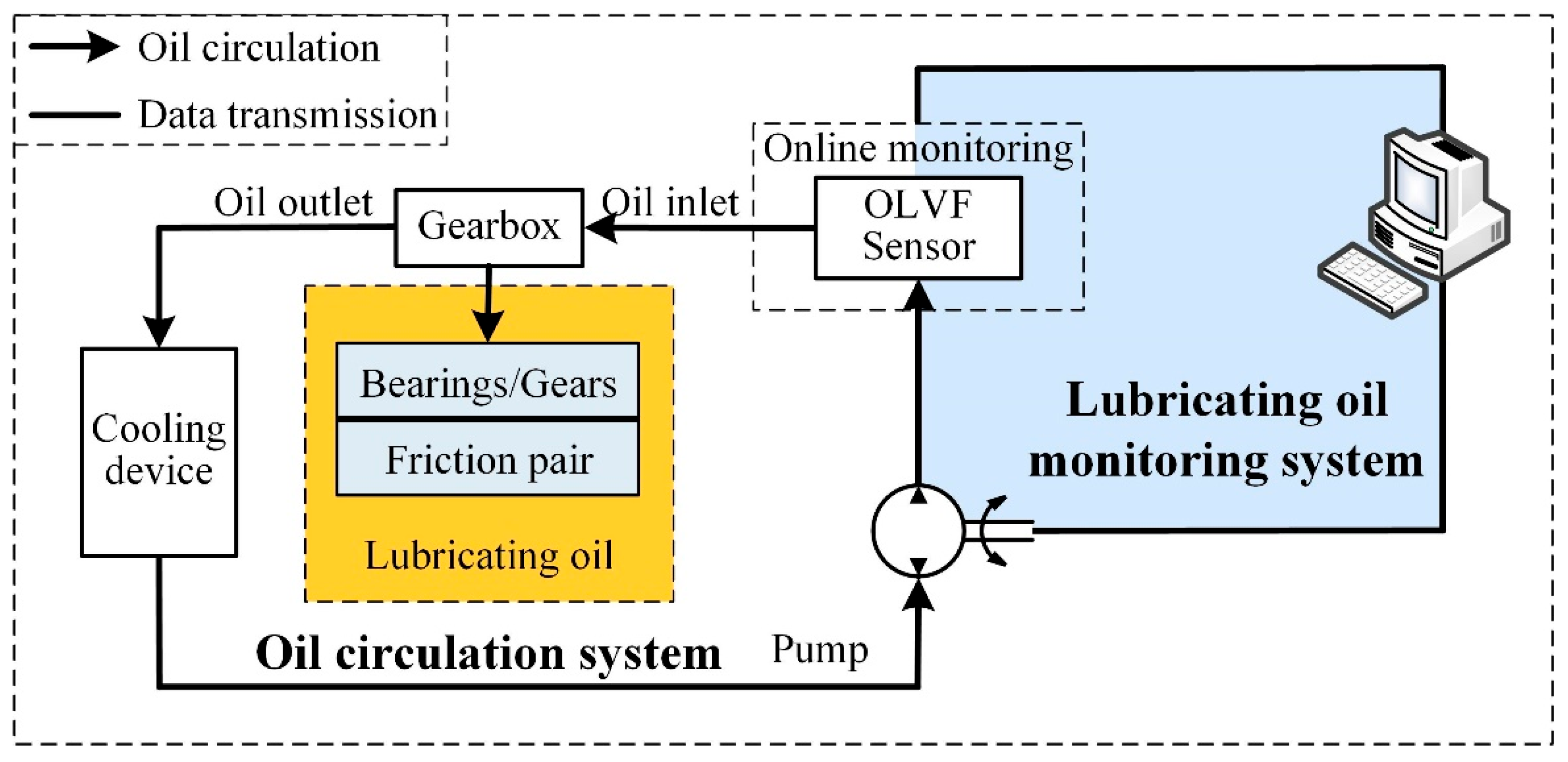
Lubricating oil monitoring technology is a sensor-based analytical technique that provides deep insights into the wear characteristics of lubricating oil [17]. Wear debris present in lubricating oil constitutes both a product of wear and an initiator of further wear [18]. Hence, as the most direct and essential carrier of information for investigating wear behavior, wear debris concentration serves as a critical and readily observable parameter for characterizing the wear state of equipment. In the present study, an online lubricating oil monitoring system was developed, the schematic representation of which is illustrated in Figure 1.
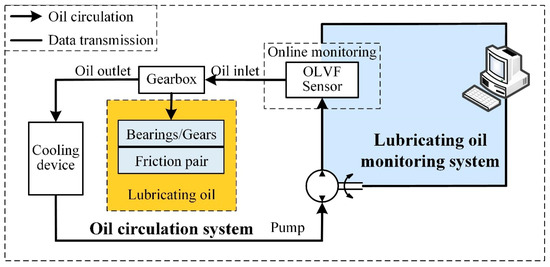
Figure 1.
Schematic diagram of the online lubricating oil monitoring system.
The system consists of an online lubricating oil monitoring sensor, a friction pair, an oil circulation system, and a data transmission system. For the online lubricating oil monitoring sensor, the Online Visual Ferrograph (OLVF) sensor [19] was selected. This sensor can capture wear particle images under three distinct light conditions: transmitted light, reflected light, and full-spectrum illumination. This multi-source imaging approach effectively minimizes false particle detection by cross-validating morphological features. Featuring sub-5-micron optical resolution, the system provides high-definition characterization of particle morphology, surface texture, and edge definition. Its optimized detection range spans 20 to 200 microns, covering critical wear particle sizes indicative of mechanical component degradation in industrial systems.
The OLVF operates on the principle of magnetic deposition and image analysis. It incorporates electromagnetic components positioned within the lubricant flow path to deposit wear particles. Images of the deposited wear particles under controlled illumination are subsequently acquired. Quantitative assessment of wear debris is achieved by calculating the relative Index of Particle Coverage Area (IPCA), as expressed by the following formula:
where is the number of object pixels of wear debris in the segmented image, is the width of the ferrograph image, and is the height of the ferrograph image.
The system operates as follows:
- (1)
- Oil Extraction: Lubricating oil is extracted from a gearbox containing bearings.
- (2)
- Cooling: The extracted oil is passed through a cooling device to reduce its temperature.
- (3)
- Monitoring: The cooled oil is then transported to the OLVF sensor, where IPCA data are detected.
- (4)
- Recirculation: After monitoring, the oil returns to the gearbox through the oil circulation system and undergoes filtration before entering the gearbox oil pool.
To ensure accurate monitoring, the system includes a cooling device to mitigate the effects of heat generated during high-speed operation of the gearbox. The physical setup of the monitoring system is shown in Figure 2.
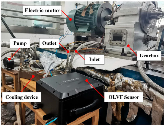
Figure 2.
Physical setup of the lubricating oil monitoring system.
In this study, a 3000 h full-lifetime test was designed, during which the ferrograph sensor continuously monitored wear particle information in the lubricating oil. To closely simulate the actual operating scenarios of aero-engines, the experiment was divided into eight different operating conditions, which were cycled according to their respective durations as shown in Table 1. These conditions encompass a range of rotational speeds (9004 to 13,741 rpm) and operational durations (approximately 10 to 54 min per cycle), reflecting the variability commonly encountered in industrial and aerospace applications.

Table 1.
Experimental operating conditions.
The selection of these specific rotational speeds and durations was based on two main considerations. First, the tested speeds cover both medium- and high-speed regimes typical of main gearbox or accessory drive shafts in modern aero-engines, where operational speeds often range from around 9000 rpm up to over 13,000 rpm. Second, the alternating duration of each speed segment reflects real-world engine operating patterns, including continuous cruise, transient acceleration/deceleration, and other mission profiles. By cycling through these variable conditions, the experiment aims to ensure that the collected data adequately represent the dynamic and complex loading environments experienced in service, thereby enhancing the reliability and applicability of the monitoring and prediction results for practical engineering use.
As shown in Table 1, the experiment covers a wide range of rotational speeds, from 9004 rpm to 13,741 rpm, and varying operating durations. Conditions 1 and 8, 2 and 7, and 3 and 6 have identical rotational speeds and durations, ensuring consistency in the experimental design.
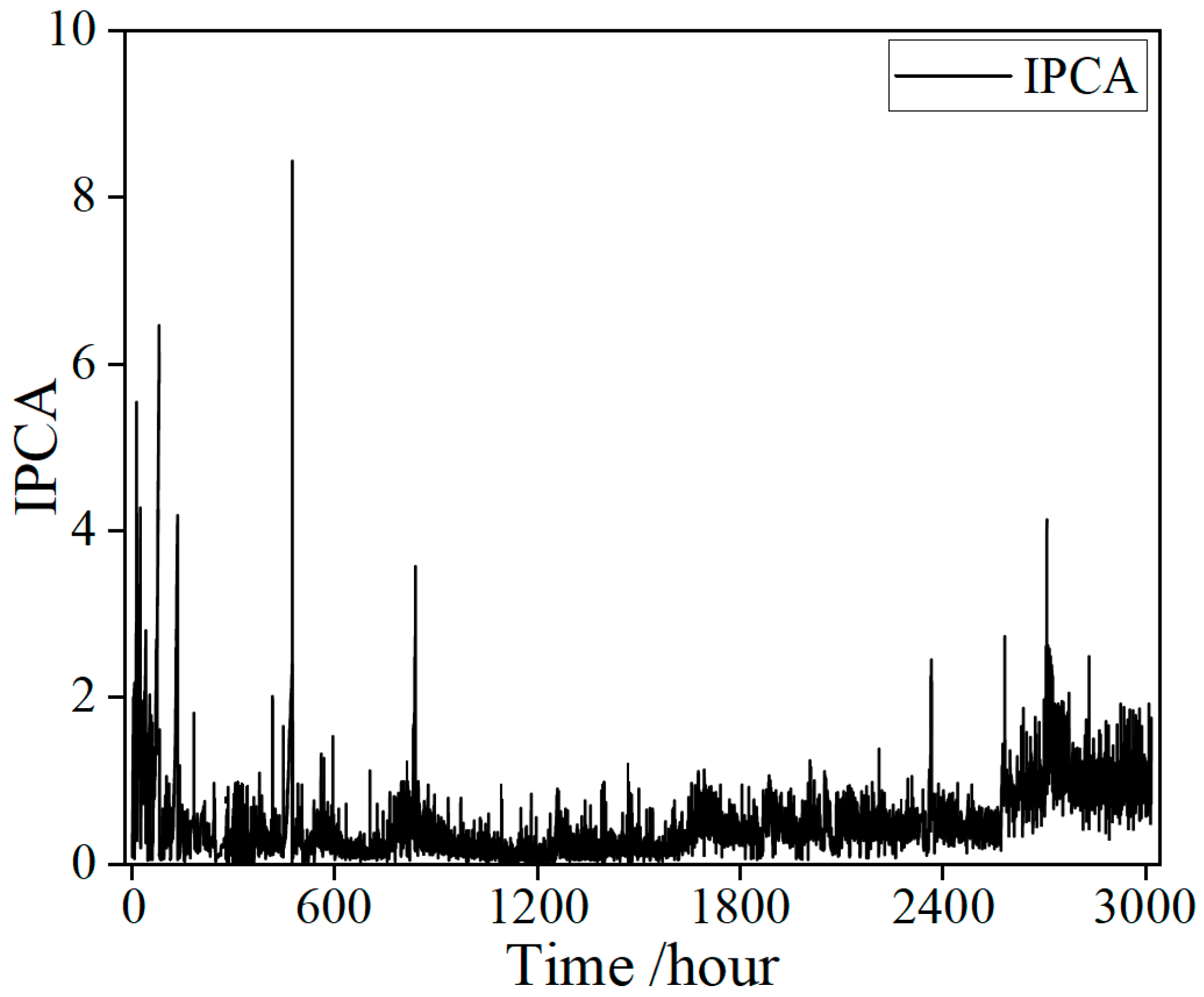
During the experiment, a large volume of oil monitoring data were collected, primarily recording the IPCA under different operating conditions. Exemplar raw signals collected from the sensor are shown in Figure 3. The IPCA exhibits distinct stage-dependent fluctuations over the 3000 h monitoring period. During the initial 100 h, the IPCA values fluctuate sharply, with multiple pronounced spikes, indicating frequent occurrences of abnormal particle generation in the early stage of the lubrication system. Subsequently, from 100 to 2600 h, the overall IPCA level decreases markedly and remains relatively stable within a lower range, suggesting that the wear state of the equipment tends to stabilize. In the later phase of the experiment, after approximately 2600 h, the IPCA rises again significantly, accompanied by several new spikes, indicating intensified wear or the emergence of new abnormal events. Overall, the IPCA curve shows pronounced volatility and sudden peaks during both the early and late stages, while remaining relatively stable in the middle phase. This trend reflects the evolution of wear throughout different life-cycle stages of the equipment.
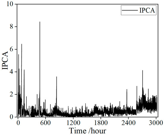
Figure 3.
Exemplar raw signals collected from the sensor.
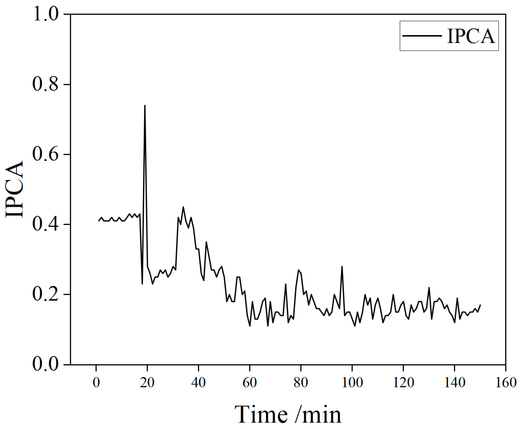
To improve data utilization and modeling efficiency, the original full-condition dataset was divided into eight subsets, each corresponding to a specific operating condition. Taking Condition 1 as an example, a segment of IPCA time-series data with a length of 150 was randomly selected from its interval as a model input sample for predicting the trend of wear particle concentration. This partitioning and sampling approach ensures comprehensive coverage of different conditions and enhances both sample diversity and training efficiency. Figure 4 shows the typical oil data history for Condition 1.
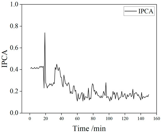
Figure 4.
Typical oil data history for Condition 1.
2.2. Problem Statement
As shown in Figure 4, from the overall trend, it can be seen that the motor starts at 20 min. In the initial stage (20–60 min), the lubricating oil shows characteristics of rapid increase followed by a sharp decline: the IPCA rises to 0.8 and then drops to 0.1. At the moment of equipment startup, the gear pair is subjected to a large torque, resulting in an instantaneous increase in IPCA. Additionally, the drastic change in IPCA during this stage is related to the gradual smoothing of asperities on the friction pair surface during the running-in process of the gear system. Subsequently, the data enter a stable period (60–150 min), where the wear state of the lubricating oil stabilizes, conforming to the time-evolution law of “initial adjustment–middle steady state”.
However, the abrasive particle concentration is influenced by factors such as lubricating oil properties, contaminants, wear particles, and wear surface roughness. Meanwhile, wear, filtration, and sedimentation effects can also introduce significant uncertainties into the monitoring data of particle concentration. Under the combined influence of external operating conditions and internal physicochemical interactions, the instantaneous changes in lubricating oil wear performance characterization data exhibit strong nonlinearity and dynamic time-varying characteristics. In practical engineering applications, the inherent complexity of lubricating oil monitoring datasets poses significant challenges for effective feature extraction and trend prediction.
Currently, the accuracy of commonly used lubricating oil wear state prediction models is primarily constrained by three technical bottlenecks. Firstly, when dealing with oil monitoring datasets with complex tribological characteristics, the accuracy of model feature selection and extraction directly affects the quality of prediction results. Secondly, after feature extraction, the ability to accurately identify key features influencing data changes from numerous features significantly impacts prediction accuracy. Finally, given the strong dynamic time-varying characteristics in oil monitoring data, accurately capturing the temporal dependencies in the data is crucial to ensuring prediction accuracy. These problems demonstrate insufficient capability in capturing dynamic relationships between lubricant performance degradation and wear progression mechanisms. When extrapolating to evolving operational conditions over extended durations, due to inadequate consideration of the nonlinear characteristics inherent to tribological systems, traditional methods also exhibit constrained generalization capabilities. Furthermore, the linear assumptions, computational complexity, and parameter selection limitations of these methods further constrain the accuracy of lubricating oil wear state prediction [20].
2.3. CNN–LSTM–Attention
To address the challenges of feature extraction and trend prediction in lubricating oil monitoring data, this study develops a more accurate CNN–LSTM–Attention model. Throughout the service life of lubricating oil, variations in particle concentration are governed by the combined effects of mechanical wear mechanisms and environmental disturbances, resulting in pronounced non-stationarity in the monitoring data. This multifactorial coupling greatly increases the complexity of extracting meaningful features from lubricant monitoring signals. CNNs (whose fundamental principles are outlined in Appendix A and described in detail in [21,22]) demonstrate notable advantages in feature extraction and are highly effective at capturing intricate local patterns. However, conventional pooling layers with coarse downsampling may lead to the loss of essential degradation features, such as the IPCA. The attention mechanism (see Appendix B and references [23,24]) dynamically assigns weights and adaptively focuses on high-information-entropy regions, thus effectively mitigating the core challenges of “feature dilution” and “noise interference” in lubricant monitoring.
Moreover, lubricant monitoring data are inherently strongly time-dependent and non-stationary, with degradation trajectories frequently exhibiting long-term dependencies, such as the autocorrelation decay of particle concentration. Compared with traditional machine learning models, which often suffer from issues like gradient vanishing and memory truncation when handling time-series data, LSTM (see Appendix C and references [25,26]) networks can adaptively capture multi-scale degradation trends in lubricant monitoring data, thereby providing robust support for temporal causal inference in lubricant condition evolution.
By combining the local feature extraction capability of CNNs with an attention mechanism, the flexibility and accuracy of extracting temporal data features are further improved, enabling CNNs to adaptively focus on key features in lubricating oil data. Subsequently, the LSTM model captures the time-series dependency in lubricating oil monitoring data, further enhancing prediction accuracy. A schematic diagram of the proposed method is shown in Figure 5.
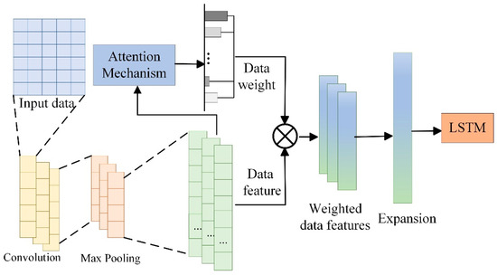
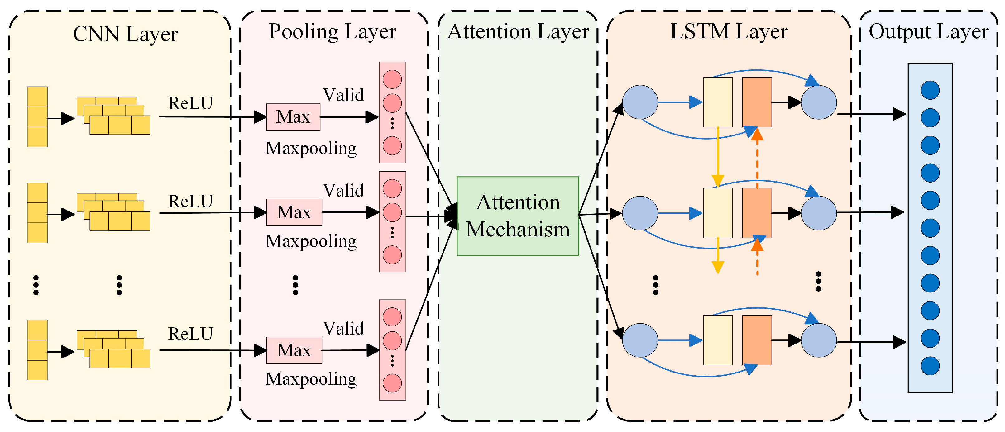
Figure 5.
Schematic diagram of the CNN–LSTM–Attention model.
As shown in Figure 5, this method realizes hierarchical feature processing of lubricating oil monitoring data through a three-stage cascaded structure of CNN–LSTM–Attention. Specifically, the CNN convolutional layer extracts spatial features of the monitoring data [27], such as the local variation patterns of IPCA (Particle Coverage Area Index). The pooling layer incorporates an attention mechanism, which can automatically identify key feature regions. The LSTM network captures the correlation in time series to understand the cumulative trend of lubricating oil wear. The attention mechanism performs secondary weighting to highlight the contribution degree of important feature channels: through learnable weight matrices (such as Query–Key matrices), it achieves adaptive allocation of feature importance. Combined with the long-term storage units of LSTM, this effectively solves the challenge of temporal dependency in time-series data and improves the accuracy and reliability of lubricating oil wear state prediction. The integration of these three methods enables the proposed model to exhibit stronger representation capability and excellent performance in lubricating oil data prediction tasks.
The proposed model employs a comprehensive feature extraction and temporal modeling pipeline to process oil monitoring data. First, two convolutional layers are defined, and each convolutional layer uses the ReLU activation function to extract the local features of lubricating oil monitoring data to enhance the nonlinear representation capability. The convolution calculation formula is as follows:
where represents the input function, represents the convolution kernel, and represents the output function. In continuous form, the convolution operation can be understood as sliding the convolution kernel over the input function and calculating the result of the convolution operation at each position.
Both convolutional layers utilize [3, 1]-shaped convolution kernels that slide across the input data with a stride of 1 to extract local features, each generating 32 feature maps (totaling 64). The convolution process computes element-wise products between the kernel and input regions, summing them to form feature maps. Subsequently, global average pooling is applied along the spatial dimensions of each feature map, producing an output vector of a length equal to the number of channels. For an input feature map of size [, , ], the pooling operation is defined as
where represents the pixel value of the c-th channel at position , while denotes the output value of that channel after pooling. The output vector of the pooling layer has a dimension of [1,1,].
Following the pooling layer, an attention mechanism module is introduced, which consists of two key steps: Squeeze and Excitation. The Squeeze step, consistent with the pooling operation, compresses the spatial dimensions (height and width ) into a single channel descriptor. This is already accomplished by the pooling layer, resulting in a feature vector of size [1,1,]. The Excitation step learns inter-channel dependencies through fully connected layers to generate a weight for each channel. Finally, the weight vector generated by the SE attention mechanism is multiplied element-wise with the original feature map to recalibrate the importance of each channel. This channel-wise weighting strategy adaptively enhances features critical to the task.
The key features processed by the attention mechanism are fed into an LSTM network, which includes
- (1)
- A sequence unfolding layer that reorganizes the data for subsequent processing.
- (2)
- A flatten layer that converts multi-dimensional data into a one-dimensional vector for input to the fully connected layer.
- (3)
- A LSTM layer with 6 units, configured to output only the result of the last time step via the “last” output mode.
- (4)
- A fully connected layer with an output dimension of 1 to process the output from the LSTM layer.
- (5)
- A regression layer that outputs the final prediction of the lubricant wear state.
The LSTM captures the temporal dynamics in the oil monitoring time-series data, and regression is performed to forecast future values, thereby enabling the prediction of the lubricant wear state.
3. Verification
3.1. Evaluation Metrics
To evaluate the performance of the time-series prediction model, three key metrics were used: Root Mean Square Error (RMSE), Mean Absolute Error (MAE), and Mean Absolute Percentage Error (MAPE). These metrics provide a quantitative basis for assessing the model’s predictive performance.
RMSE: Measures the square root of the average squared differences between predicted and actual values. It is a widely used metric for evaluating prediction accuracy.
MAE: Computes the average absolute differences between predicted and actual values, providing a direct measure of prediction error.
MAPE: Calculates the average absolute percentage error between predicted and actual values, providing a measure of the relative magnitude of prediction error.
Given the complexity and uniqueness of the LSTM model when dealing with time-series data, the three-evaluation metrics are applied to comprehensively assess the performance of the time-series prediction model. The formulas for these metrics are shown in Table 2.
Table 2.
Evaluation indicators.
3.2. Model Verification
To validate the effectiveness of the proposed CNN–LSTM–Attention model, the oil monitoring data were preprocessed and split into training and testing sets. Specifically, thirty-five sets of historical data were used for training, and eight sets were randomly selected for testing. The verification process is illustrated in Figure 6.

Figure 6.
Verification flowchart.
The proposed model was implemented utilizing MATLAB version R2022b on a machine equipped with an NVIDIA GeForce RTX 3080 GPU, an Intel(R) Core (TM) i7-12700F CPU @2.10 GHz, and 32.0 GB of system memory.
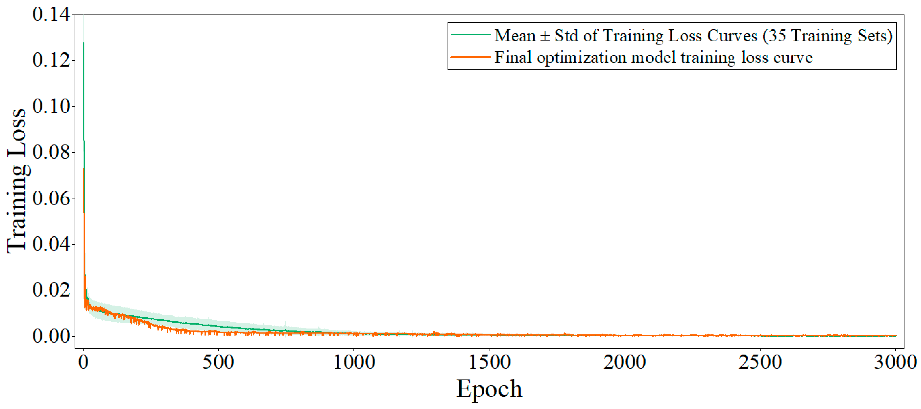
Throughout this process, the input data undergo rigorous preprocessing, including reshaping and normalization, to meet the requirements of the model. Model training is optimized using the Adam optimizer [28], which adaptively adjusts learning rates to enhance both convergence speed and training stability. The mean squared error (MSE) loss function is employed to minimize the discrepancy between predicted and actual values. The initial learning rate is set to 0.005 and decays by a factor of 0.9 every 500 epochs to help the model escape local minima and achieve better convergence. The model is trained for up to 3000 epochs, with the training set shuffled at each epoch to improve generalization. The final optimized model is obtained by iteratively training on the entire training set, and the weights are saved when the loss converges or the maximum number of epochs is reached. Since the training processes of all test samples display similar trends, this study selects a randomly chosen representative sample (Sample 3) and presents, as an example, the mean and standard deviation of the training loss curves of its 35 training sets, along with the training loss curve of the finally optimized model. As shown in Figure 7, the x-axis indicates the number of training epochs, and the y-axis represents the training loss. The curve shows that the training loss drops rapidly at the beginning and gradually stabilizes after about 500 epochs, remaining at a low level thereafter. This suggests that the model converges well without obvious overfitting. Overall, the figure intuitively reflects the effectiveness and convergence speed of the training process.
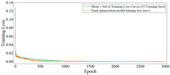
Figure 7.
Training loss curve (test sample 3 as an example).
The final model adopts CNN–LSTM–Attention regression architecture. The input layer receives a sliding window of length 10 from the univariate IPCA time series (shape: [1,10]. A sample input can be formatted as [0.85,0.86,0.92,0.99,1.08,1.15,1.1,0.72,0.83]), which is transformed by a sequence folding layer to facilitate subsequent convolution operations. The first convolutional layer uses 3 × 1 kernels with 32 output channels to extract local temporal features, followed by a ReLU activation. The second convolutional layer, also with 3 × 1 kernels and 64 channels, captures higher-level features, again followed by a ReLU activation. A global average pooling layer aggregates features across each channel, yielding a 64-dimensional channel descriptor. The subsequent Squeeze-and-Excitation (SE) [29] channel attention module consists of two fully connected layers (16 and 64 units), with a final sigmoid activation to produce a 64-dimensional attention weight vector for adaptive channel-wise feature recalibration. The attention-weighted features are then reshaped via sequence unfolding and flattening layers to a format suitable for the LSTM layer, which contains six units and outputs only the last time step to model temporal dependencies. Finally, a fully connected layer predicts the next IPCA value, and a regression output layer computes the loss for model training.
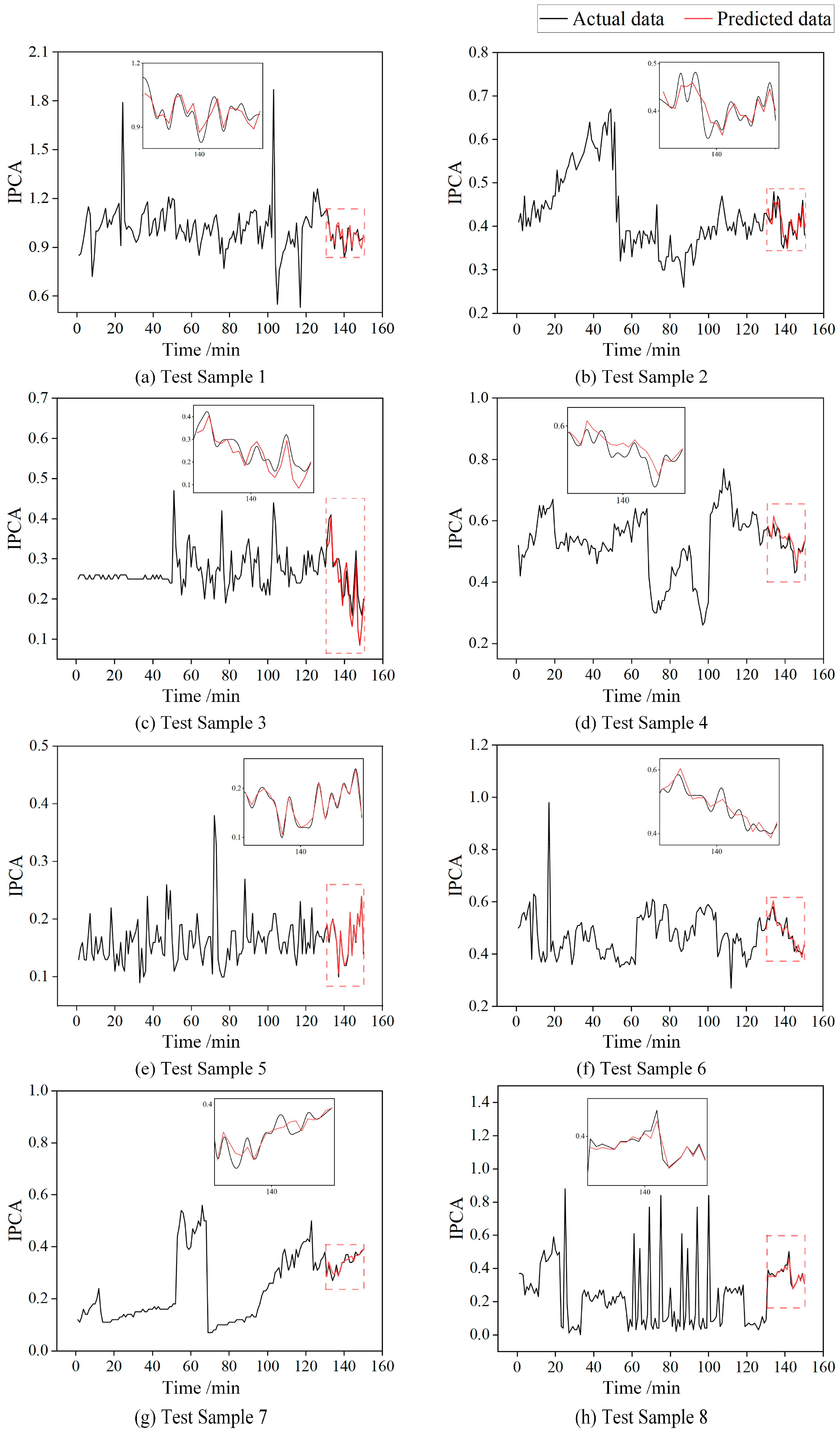
This integrated approach systematically addresses feature extraction, importance weighting, and temporal modeling in a unified framework for accurate oil condition monitoring. The model takes a time series of 150 IPCA sampling points as input, with the first 80% used for training and the model outputting the predicted IPCA values for the last 20%. For final evaluation, the model’s predicted IPCA values at the last 20 sampling points are compared with the actual measured values, which better reflect the model’s ability to capture long-term trends and handle extreme scenarios. The prediction results for the eight test samples are shown in Figure 8.
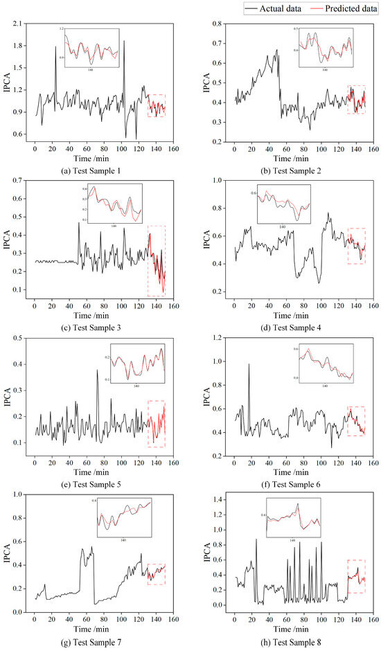
Figure 8.
The prediction results for the eight test samples.
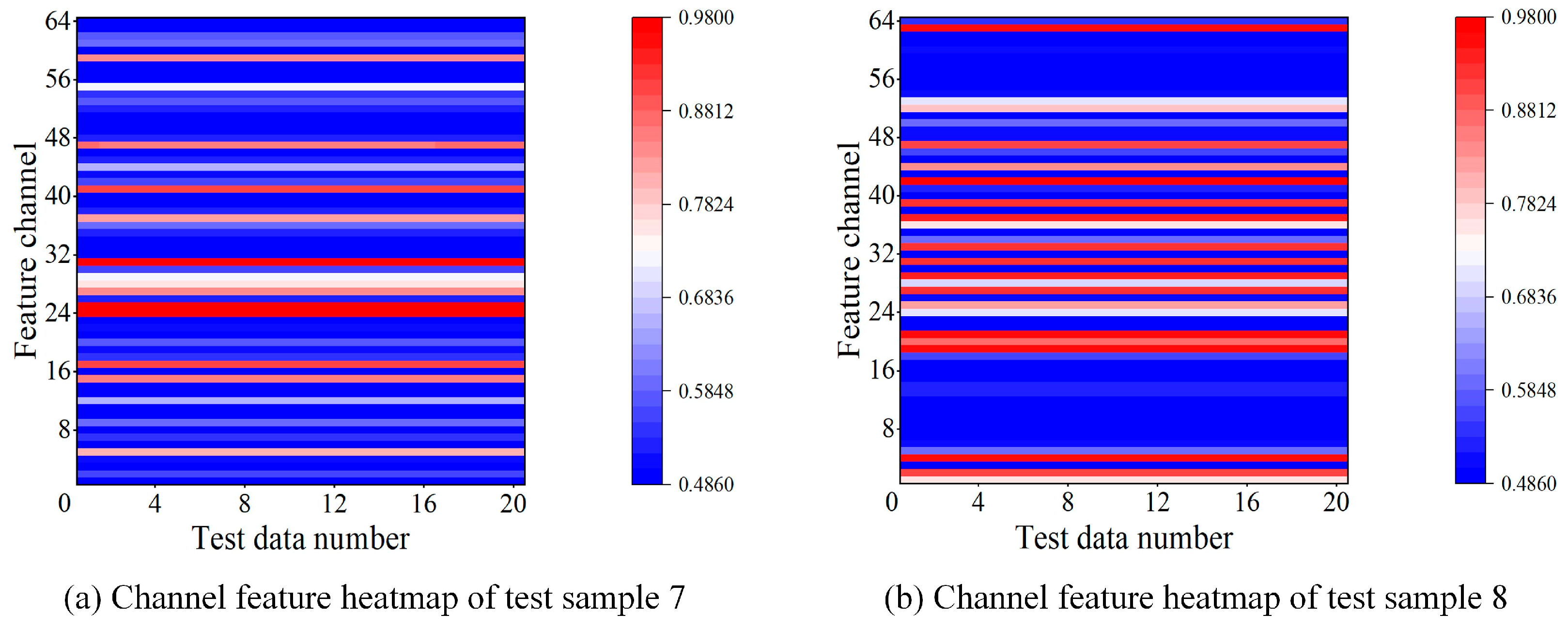
As shown in Figure 8, test samples 1, 4, 5, 6, and 8 exhibit stable or mildly fluctuating IPCA values, indicating a steady wear stage; test samples 2 and 3 start with high IPCA values that gradually decrease, characteristic of the running-in phase; and test sample 7 shows a continuous IPCA increase at the end, suggesting transient disturbance or abnormal wear. Overall, the model demonstrates high-precision trend prediction capability across all eight test samples. Figure 9 shows the channel attention heatmaps of test samples 7 and 8, respectively.
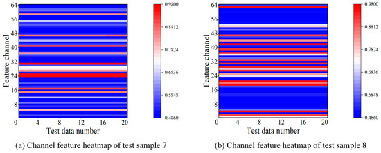
Figure 9.
Distribution of channel attention weights on the test sample.
It can be observed that the model consistently assigns high weights to some feature channels during the prediction process, indicating that the features extracted by these channels play a critical role in wear state prediction.
The evaluation metrics for the four test samples are summarized in Table 3.
Table 3.
Evaluation metrics summary.
As shown in Table 3, the RMSE, MAE, and MAPE values for all test samples are relatively small, indicating that the model’s predictions are highly accurate. This demonstrates the effectiveness of the proposed CNN–LSTM–Attention model in predicting lubricating oil wear states.
4. Discussion and Outlook
4.1. Performance Discussion of Proposed Method
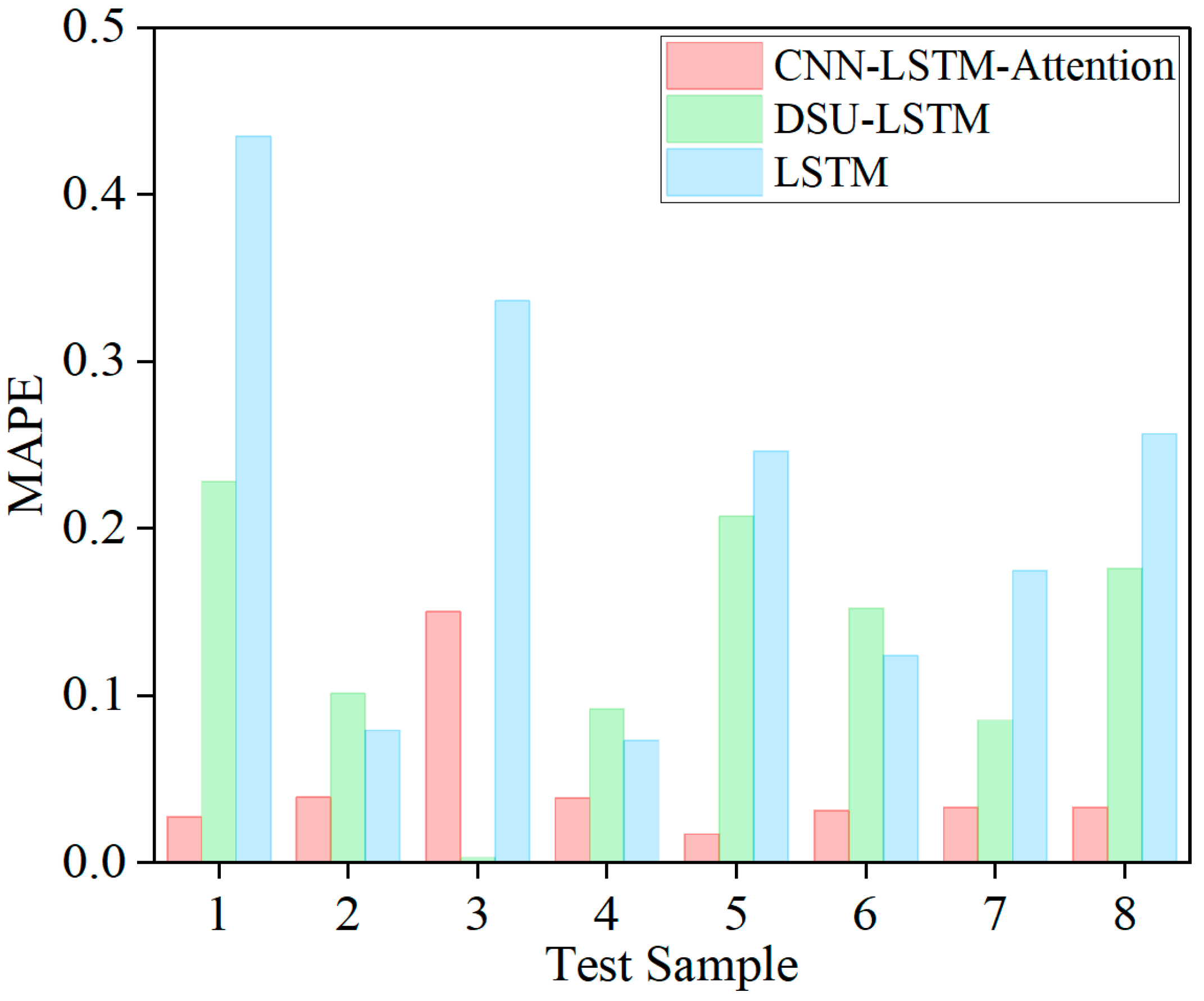
To further validate the performance of the proposed model, it was compared with several existing models, including DSU–LSTM (Distribution of System Uncertainty) [1] and LSTM [15]. The average evaluation metrics for the four test samples are shown in Table 4. The MAPE results of the three models on eight test samples are shown in Figure 10. There are notable differences in MAPE across all test samples among the three models. The proposed CNN–LSTM–Attention model consistently achieves the lowest MAPE, outperforming both the DSU–LSTM and traditional LSTM models. This demonstrates its superior predictive accuracy and robustness for wear state estimation.
Table 4.
Comparison of evaluation metrics.
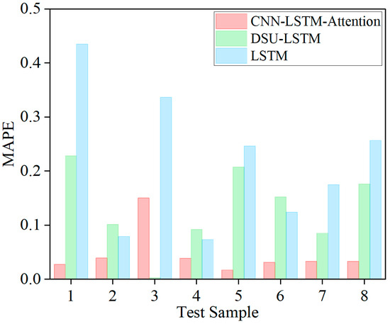
Figure 10.
Comparison of test set MAPE for three models.
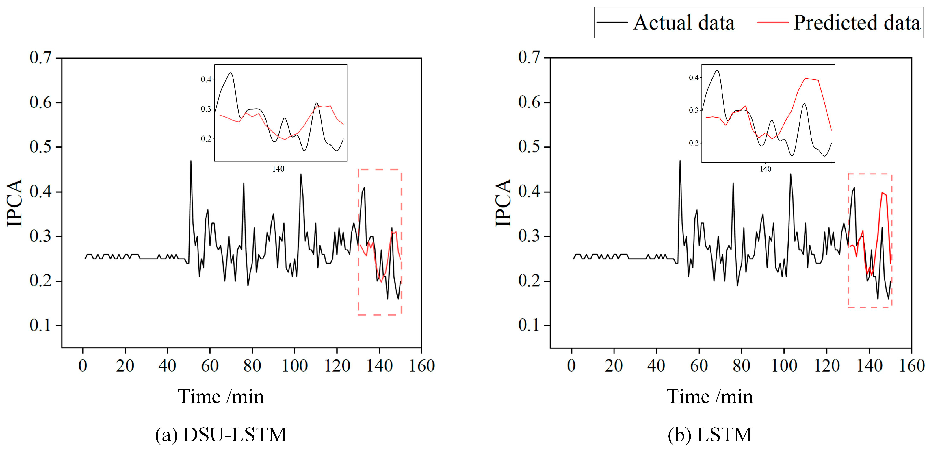
Compared with commonly used machine learning-based wear state prediction methods (as shown in Figure 11), the proposed method integrates the powerful local feature extraction capability of CNNs, the advantage of LSTM in handling time-series dependencies, and the adaptive focusing characteristics of the attention mechanism. This allows it to effectively extract detailed features from oil monitoring data, dynamically adjust the weights of different features through the self-attention mechanism to ensure the model prioritizes information critical for prediction, and finally further process time-series relationships via LSTM. As shown in Figure 8c, the prediction results exhibit significantly higher consistency with actual values. The method accurately captures changes in real data both in overall trends and detailed fluctuations, fully demonstrating the theoretical advantages of this approach and its stronger capability in feature capture and trend prediction when dealing with lubricating oil monitoring data.
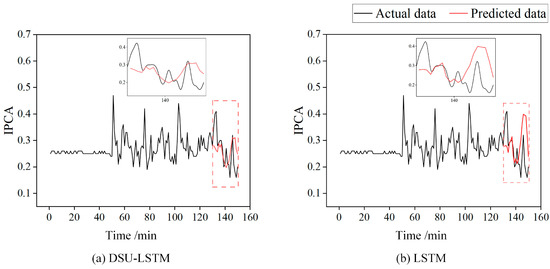
Figure 11.
Comparison of wear state prediction models.
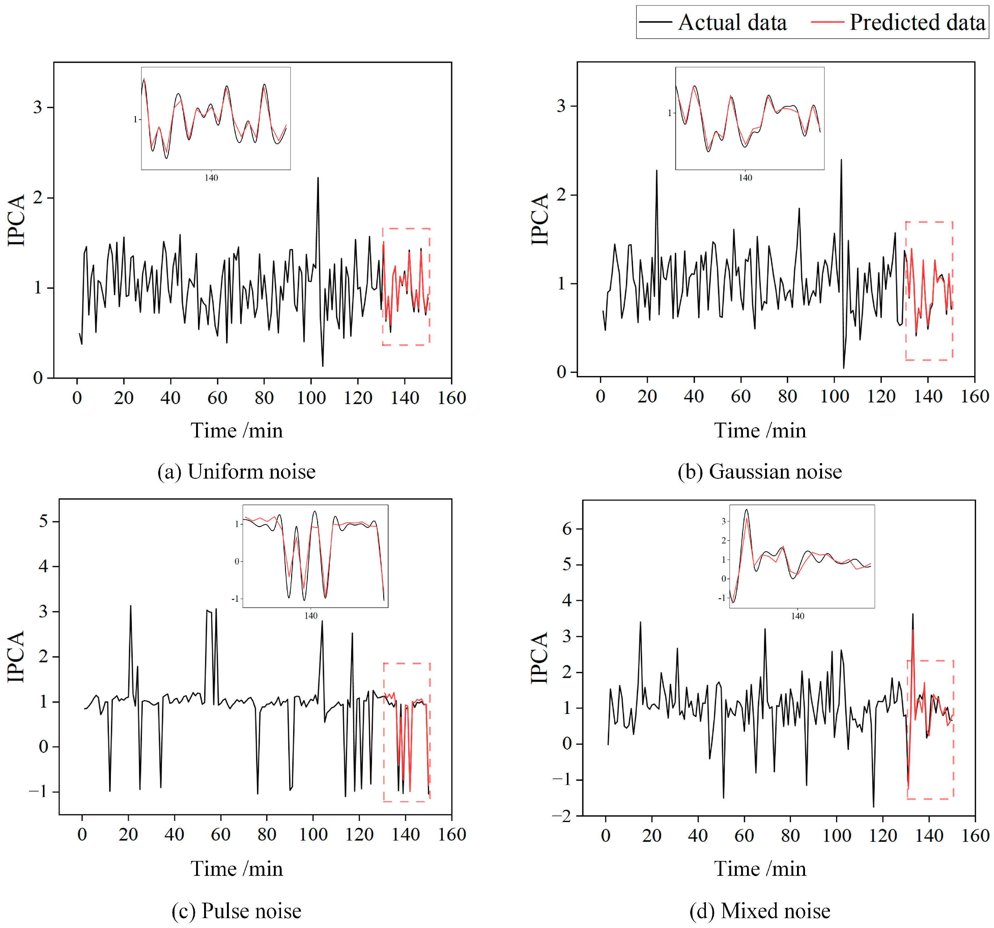
To ensure the model’s performance, we manually added Uniform noise, Gaussian noise, Pulse noise, and Mixed noise to the oil monitoring data to test the model’s reliability in handling noisy or abnormal data. As shown in Figure 12, although the data fluctuate violently and contain some outliers, the model’s prediction curve still fits the main trend of the actual curve well. This demonstrates that the model maintains considerable prediction accuracy and good anti-interference ability in complex noise environments and can accurately predict noisy oil monitoring data.
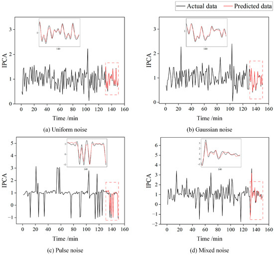
Figure 12.
Prediction results under different noise conditions.
4.2. Outlook
The CNN–LSTM–Attention model proposed in this study achieves wear state prediction of mechanical equipment based on lubricating oil monitoring data, enabling early operational maintenance. It is suitable for lubricating oil monitoring time-series data with complex coupling characteristics and can still ensure high prediction accuracy under complex noise environmental conditions. However, due to experimental environment limitations, this study only collected IPCA data of one type of lubricating oil in a test bench. Additional experiments using broader and more diverse datasets could provide a more comprehensive evaluation of the model’s robustness. Furthermore, the scarcity of data prevents the support of newer architectures such as Gated Recurrent Units (GRUs), Temporal Convolutional Networks (TCNs), or Transformer-based models. Future work should conduct more extensive benchmark analyses and include hyperparameter sensitivity studies to ensure model robustness and avoid potential overfitting issues.
5. Conclusions
This study presents a novel CNN–LSTM–Attention hybrid model for high-precision prediction of wear state in lubricating oil monitoring systems. The key innovations are as follows:
- Advanced Feature Extraction: The CNN module, through hierarchical convolutional layers, effectively captures high-dimensional spatial and temporal features from oil monitoring data, automatically learning complex nonlinear degradation patterns and reducing reliance on manual feature engineering.
- Dynamic Feature Importance Weighting: The introduction of a self-attention mechanism enables the model to adaptively identify and focus on diagnostically critical features while effectively suppressing irrelevant noise. This greatly enhances the model’s interpretability and predictive reliability under variable operating conditions.
- Long-Term Temporal Dependency Modeling: The LSTM component effectively models long-term dependencies in monitoring data, accurately tracking the temporal evolution of wear processes and addressing the limitations of conventional approaches in long-term degradation prediction.
In practical tests across eight samples, the proposed model demonstrated excellent and stable predictive performance. Specifically, it achieved a low MAPE of 0.046, which is significantly better than the comparison models DSU–LSTM (0.131) and LSTM (0.216). These results indicate that the method offers not only high accuracy, but also strong adaptability and generalization capability.
In summary, the CNN–LSTM–Attention model provides a robust technical foundation for the predictive maintenance of industrial equipment. It also shows great potential for applications in other fluid condition monitoring and degradation trend prediction tasks, supporting intelligent operation and health management in complex engineering scenarios.
Author Contributions
Methodology, Y.D., H.W., and Y.Z.; Software, T.S. and H.W.; Validation, Y.D., H.W., and S.C.; Writing—original draft, Y.D., H.W., and T.S.; Writing—review and editing, Y.D., J.W., and C.Z.; Supervision, Y.Z., J.W., and C.Z.; Funding acquisition, Y.D. All authors have read and agreed to the published version of the manuscript.
Funding
This research was supported by the National Natural Science Foundation of China (Grant No. 52305132), Xi’an University of Technology, China (No. 102-451123002), and the project of Shaanxi Key Laboratory of Mine Electromechanical Equipment Intelligent Detection and Control, Xi’an University of Science and Technology (No. SKL-MEEIDC202403).
Data Availability Statement
The raw data supporting the conclusions of this article will be made available upon reasonable request.
Conflicts of Interest
The authors declare no conflicts of interest.
Abbreviations
The following abbreviations are used in this manuscript:
| CNN | Convolutional Neural Network |
| LSTM | Long Short-Term Memory |
| AI | Artificial Intelligence |
| RUL | Remaining Useful Life |
| WPM | Wiener Process Model |
| HMM | Hidden Markov Hodel |
| CRF | Conditional Reliability Function |
| MRL | Mean Remaining Life |
| IPCA | Index of Particle Coverage Area |
| ANN | Artificial Neural Network |
| OLVF | Online Visual Ferrograph |
| MSE | Mean Squared Error |
| RMSE | Root Mean Square Error |
| MAE | Mean Absolute Error |
| MAPE | Mean Absolute Percentage Error |
| DSU | Distribution of System Uncertainty |
| GRU | Gated Recurrent Unit |
| TCN | Temporal Convolutional Network |
Appendix A. Architecture of CNN Model
A CNN is a deep learning neural network, and its basic fundamental architecture is illustrated in Figure A1. The basic structure of a CNN includes an input layer, convolutional layers, pooling layers, fully connected layers, and an output layer. Each of these layers has unique advantages, collectively contributing to the CNN’s powerful capability in handling complex data [21,22].

Figure A1.
Architecture of a convolutional neural network.
Figure A1.
Architecture of a convolutional neural network.
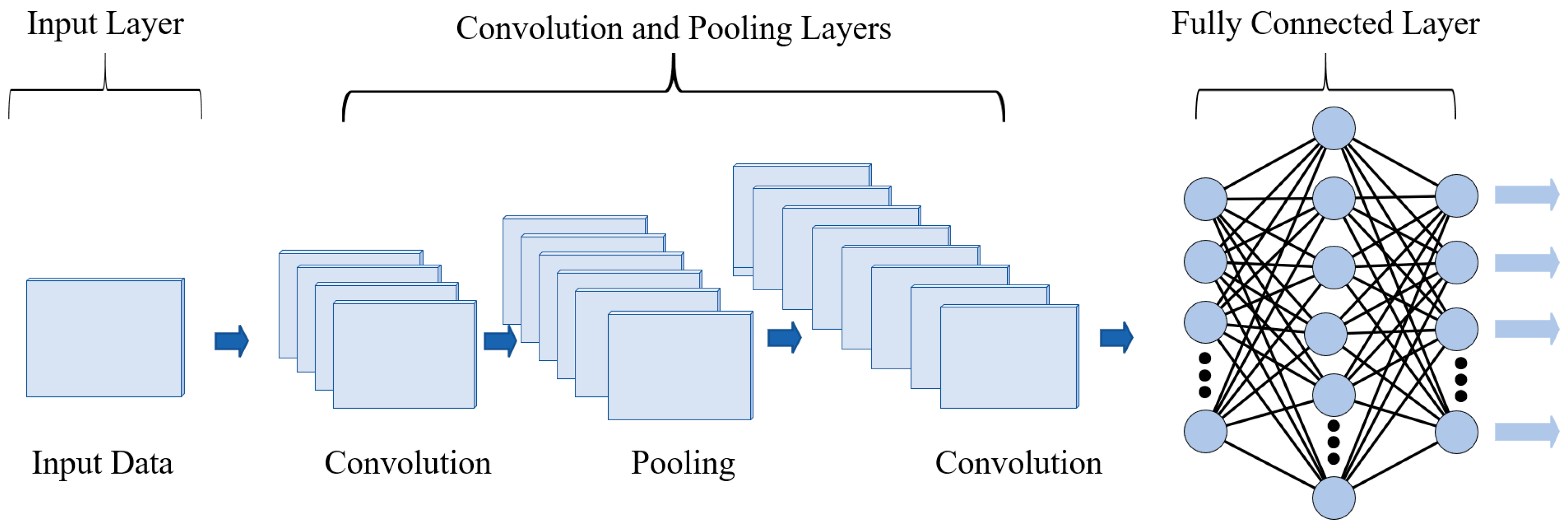
- (1)
- Input layer
The input layer, as the first layer of the CNN, undertakes the important task of receiving raw multi-dimensional data. It performs necessary preprocessing operations, including mean removal and normalization, to ensure the stability and consistency of the data. In addition, the input layer converts the raw data into a format that can be processed by the neural network and passes the preprocessed data to the subsequent convolutional layers for further feature extraction.
- (2)
- Convolutional layer
The convolutional layer is primarily responsible for extracting multi-level features from oil data. Multi-level features of the input data are extracted through convolution kernels. As shown in Figure A2, a 3 × 3 convolution kernel slides across the input matrix at a specified stride, computing the sum of element-wise products in local regions to generate feature values. This kernel traverses the data from left to right and top to bottom, ultimately forming a convolutional feature map that encapsulates diverse feature information from the input data.
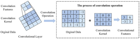
Figure A2.
Operation of the convolutional layer. (* represents convolution operation).
Figure A2.
Operation of the convolutional layer. (* represents convolution operation).
For an input feature map with size , after applying edge pixel padding of size and then performing convolution with a kernel of size and stride s, the dimensions (length and width) of the output feature map can be calculated using the following formula:
- (3)
- Pooling layer
The pooling layer is a downsampling operation in a convolutional neural network. It mainly reduces the dimensionality of the feature map through methods such as max pooling and average pooling, reducing computational complexity while retaining important feature information.
- (4)
- Fully connected layer
The fully connected layer is located after the convolutional and pooling layers. Its main task is to integrate and process the feature information extracted by these layers and transform local features into global features through linear transformation and activation functions.
Appendix B. Attention Mechanism
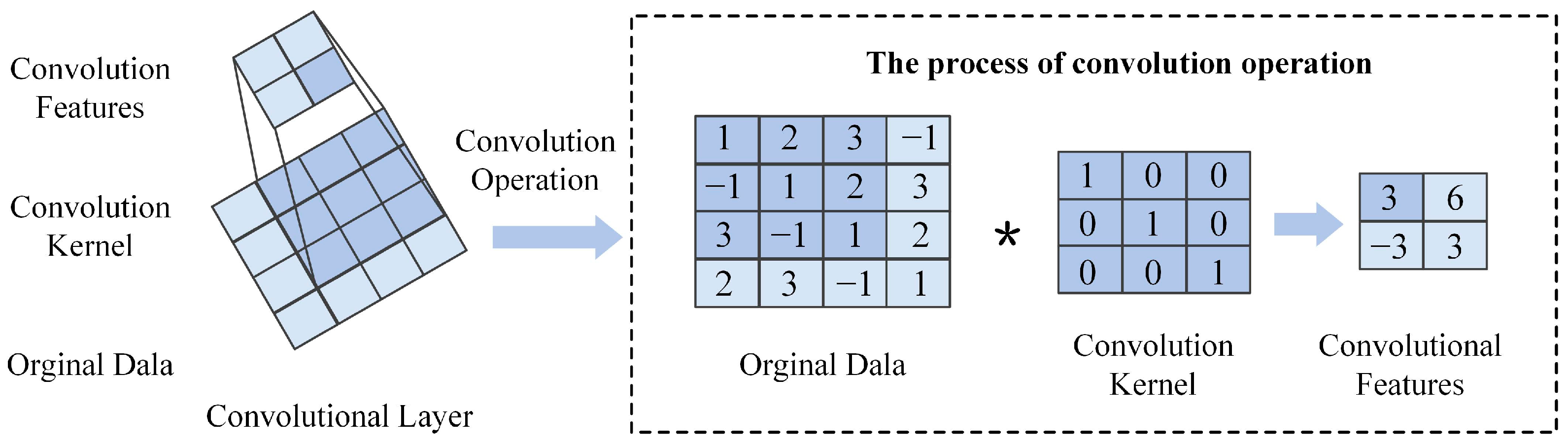
The core idea of the attention mechanism [23] is to enable neural networks to dynamically allocate attention to different parts of the input sequence, assigning higher weights to more critical information. In this study, we employ a self-Attention mechanism [24]; by calculating the correlations among different parts of the input sequence, it dynamically adjusts the feature weights, enhancing the model’s sensitivity to key features, which is illustrated in Figure A3.
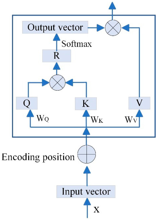
Figure A3.
Schematic diagram of the self-attention structure.
Figure A3.
Schematic diagram of the self-attention structure.
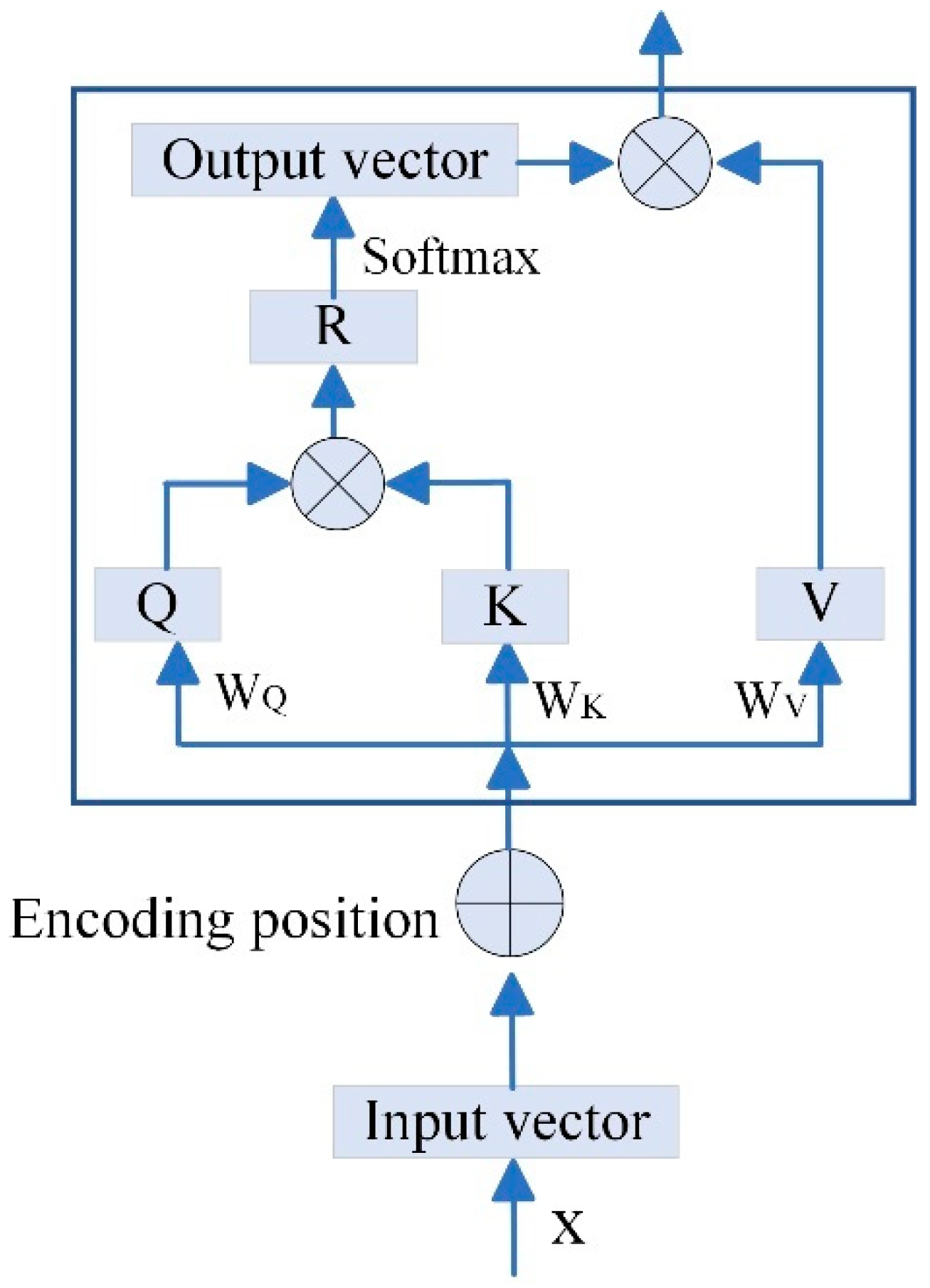
As shown in Figure A3, the input tensor is represented by , where , , and are the learnable parameters of the self-attention model. The self-attention mechanism computes new features through the following steps.
- (1)
- Query, key, and value calculation
The input tensor is transformed into three components, Query (), Key (), and Value (), through linear transformations.
These components are used to compute attention weights.
- (2)
- Attention score calculation
Attention scores are computed by taking the dot product of and , which captures the relationships between different parts of the input sequence.
Here, represents the attention scores, which quantify the importance of each part of the sequence relative to others.
- (3)
- Normalization and Softmax
The obtained local relationship matrix is normalized, and the Softmax function is applied along each channel dimension to ensure that the sum of all attention weights is 1. The output of the Softmax is then multiplied by the vector. This process enhances the representation of the key feature vectors in the image. Finally, the output of the self-attention module is obtained through the following calculation:
where is the transpose of , and is the dimension of .
- (4)
- Weighted sum of values
The final output of the self-attention mechanism is computed as a weighted sum of the value vectors, where the weights are the attention scores. This process enhances the representation of key features in the input sequence, allowing the model to focus on the most important information.
The self-attention mechanism enables the model to dynamically adjust the importance of different features in the input sequence, making it particularly effective for handling complex and time-varying data, such as lubricating oil monitoring data.
Appendix C. LSTM Model
The schematic diagram of the LSTM model is shown in Figure A4, with its core components including the forget gate, input gate, output gate, cell state, and hidden state. These components work together to control the flow of data information through gating mechanisms, enabling LSTM to effectively capture and process long-term dependencies in sequential data [25,26].
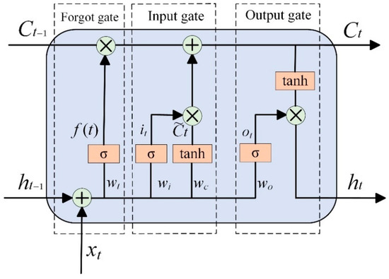
Figure A4.
Schematic diagram of the LSTM model.
Figure A4.
Schematic diagram of the LSTM model.
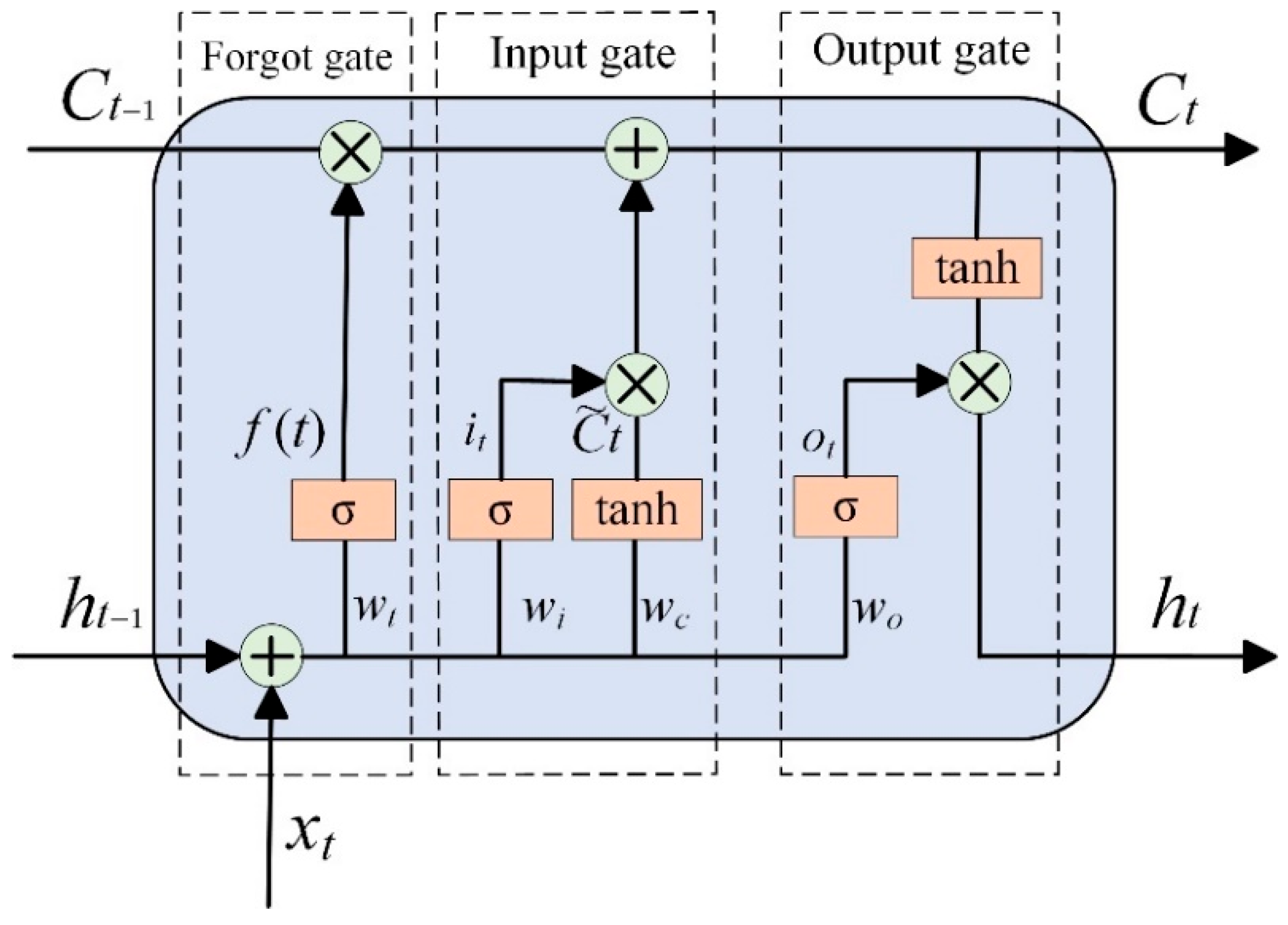
In Figure A4, represents the current time step; represents the previous time step; represents the data of the current time series; and represent the states of the long-term memory unit at the previous and current time steps, respectively; and represent the hidden states at the previous and current time steps, respectively; represents the sigmoid function, used to control the flow of information; , , , and represent the weight parameters of the forget gate, input gate, current state calculation, and output gate, respectively; and represent the input and output proportions selected by the output gate, respectively; and is the temporary state at the current time step, calculated based on the current input and the previous hidden state . Finally, the hidden state is calculated based on the current cell state and the output gate proportion .
The forget gate is the first control gate in the LSTM model, screen historical memory , and the input gate fuses current features to generate a candidate state . The unit state is updated to , and the output gate generates a hidden state based on . The specific calculation formulas are as follows:
In summary, the LSTM model, through its unique gating mechanism and unit state design, can effectively handle and predict long-term dependencies in sequential data, enabling the extraction of multi-scale wear features from transient changes in the overall trend of abrasive particles and providing time-series perception modeling capabilities for predicting lubricant degradation.
References
- Du, Y.; Zhang, Y.; Shao, T.; Zhang, Y.; Cui, Y.; Wang, S. DSU-LSTM-Based Trend Prediction Method for Lubricating Oil. Lubricants 2024, 12, 289. [Google Scholar] [CrossRef]
- Czichos, H. Tribology: A Systems Approach to the Science and Technology of Friction, Lubrication, and Wear; Elsevier: Amsterdam, The Netherlands, 2009. [Google Scholar]
- Du, Y.; Duan, C.; Wu, T. Replacement scheme for lubricating oil based on Bayesian control chart. IEEE Trans. Instrum. Meas. 2020, 70, 1–10. [Google Scholar] [CrossRef]
- Wang, S.; Han, Z.; Wei, H. An integrated knowledge and data model for adaptive diagnosis of lubricant conditions. Tribol. Int. 2024, 199, 109914. [Google Scholar] [CrossRef]
- Badihi, H.; Zhang, Y.; Jiang, B. A comprehensive review on signal-based and model-based condition monitoring of wind turbines: Fault diagnosis and lifetime prognosis. Proc. IEEE 2022, 110, 754–806. [Google Scholar] [CrossRef]
- Pan, Y.; Liang, B.; Yang, L. Spatial-temporal modeling of oil condition monitoring: A review. Reliab. Eng. Syst. Safe 2024, 248, 110182. [Google Scholar] [CrossRef]
- Pan, Y.; Han, Z.; Wu, T. Remaining useful life prediction of lubricating oil with small samples. IEEE Trans. Ind. Electron. 2022, 70, 7373–7381. [Google Scholar] [CrossRef]
- Du, Y.; Wu, T.; Makis, V. Parameter estimation and remaining useful life prediction of lubricating oil with HMM. Wear 2017, 376, 1227–1233. [Google Scholar] [CrossRef]
- Wakiru, J.M.; Pintelon, L.; Muchiri, P.N. A review on lubricant condition monitoring information analysis for maintenance decision support. Mech. Syst. Signal Proc. 2019, 118, 108–132. [Google Scholar] [CrossRef]
- Liu, Z.; Wang, H.; Hao, M. Prediction of RUL of Lubricating Oil Based on Information Entropy and SVM. Lubricants 2023, 11, 121. [Google Scholar] [CrossRef]
- Afrand, M.; Najafabadi, K.N.; Sina, N. Prediction of dynamic viscosity of a hybrid nano-lubricant by an optimal artificial neural network. Int. Commun. Heat Mass Transf. 2016, 76, 209–214. [Google Scholar] [CrossRef]
- Wang, H.; Zuo, H.; Liu, Z. Online monitoring of oil wear debris image based on CNN. Mech. Ind. 2022, 23, 9. [Google Scholar] [CrossRef]
- Sun, J.; Bu, J.; Guo, X. Intelligent Wear Condition Prediction of Ball Bearings Based on Convolutional Neural Networks and Lubricating Oil. J. Fail. Anal. Prev. 2024, 24, 1854–1864. [Google Scholar] [CrossRef]
- Su, Y.; Li, D.; Wang, H.; He, C.; Yang, K. Classification and prediction of wear state based on unsupervised learning of online monitoring data of lubricating oil. In Proceedings of the 2021 3rd International Conference on Environmental Prevention and Pollution Control Technologies (EPPCT), Zhuhai, China, 15–17 January 2021. [Google Scholar]
- Li, D.; Gao, H.; Yang, K. Abnormal identification of oil monitoring based on LSTM and SVDD. Wear 2023, 526, 204793. [Google Scholar] [CrossRef]
- Yin, F.; He, Z.; Nie, S.; Ji, H.; Ma, Z. Tribological properties and wear prediction of various ceramic friction pairs under seawater lubrication condition of different medium characteristics using CNN-LSTM method. Tribol. Int. 2023, 189, 108935. [Google Scholar] [CrossRef]
- Zhu, X.; Zhong, C.; Zhe, J. Lubricating oil conditioning sensors for online machine health monitoring—A review. Tribol. Int. 2017, 109, 473–484. [Google Scholar] [CrossRef]
- Tambadou, M.S.; Chao, D.; Duan, C. Lubrication oil anti-wear property degradation modeling and remaining useful life estimation of the system under multiple changes operating environment. IEEE Access 2019, 7, 96775–96786. [Google Scholar] [CrossRef]
- Wu, T.H.; Mao, J.H.; Wang, J.T.; Wu, J.Y.; Xie, Y.B. A new on-line visual ferrograph. Tribol. Trans. 2009, 52, 623–631. [Google Scholar] [CrossRef]
- Tanwar, M.; Raghavan, N. Lubricating oil remaining useful life prediction using multi-output Gaussian process regression. IEEE Access 2020, 8, 128897–128907. [Google Scholar] [CrossRef]
- Chauhan, R.; Ghanshala, K.K.; Joshi, R.C. Convolutional neural network (CNN) for image detection and recognition. In Proceedings of the 2020 1st International Conference on Secure Cyber Computing and Communication (ICSCCC), Jalandhar, India, 15–17 December 2018; IEEE: Piscataway, NJ, USA, 2018; pp. 278–282. [Google Scholar]
- Wen, S.Z.; Huang, P. Principles of Tribology; Qinghua University Press: Beijing, China, 2012. [Google Scholar]
- Lv, H.; Chen, J.; Pan, T. Attention mechanism in intelligent fault diagnosis of machinery: A review of technique and application. Measurement 2022, 199, 111594. [Google Scholar] [CrossRef]
- Yang, B.; Wang, L.; Wong, D. Convolutional Self-Attention Networks. arXiv 2019, arXiv:1904.03107. [Google Scholar]
- Elsworth, S.; Güttel, S. Time Series Forecasting Using LSTM Networks: A Symbolic Approach. arXiv 2020, arXiv:2003.05672. [Google Scholar]
- Wang, Y.; Zhu, S.; Li, C. Research on multistep time series prediction based on LSTM. In Proceedings of the 2019 3rd International Conference on Electronic Information Technology and Computer Engineering (EITCE), Xiamen, China, 18–20 October 2019; IEEE: Piscataway, NJ, USA, 2020; pp. 1155–1159. [Google Scholar]
- Fan, H.W.; Xue, C.Y.; Ma, J.T.; Cao, X.G.; Zhang, X.H. A novel intelligent diagnosis method of rolling bearing and rotor composite faults based on vibration signal-to-image mapping and CNN-SVM. Meas. Sci. Technol. 2023, 34, 044008. [Google Scholar]
- Ogundokun, R.O.; Maskeliunas, R.; Misra, S. Improved CNN based on batch normalization and adam optimizer. In Proceedings of the 2020 22nd International Conference on Computational Science and Its Applications(ICCSA), Malaga, Spain, 4–7 July 2022; pp. 593–604. [Google Scholar]
- Hu, J.; Shen, L.; Sun, G. Squeeze-and-excitation networks. In Proceedings of the 2018 36th IEEE Conference on Computer Vision and Pattern Recognition (CVPR), Salt Lake City, UT, USA, 18–23 June 2018; IEEE: Piscataway, NJ, USA, 2018; pp. 7132–7141. [Google Scholar]


Disclaimer/Publisher’s Note: The statements, opinions and data contained in all publications are solely those of the individual author(s) and contributor(s) and not of MDPI and/or the editor(s). MDPI and/or the editor(s) disclaim responsibility for any injury to people or property resulting from any ideas, methods, instructions or products referred to in the content. |
© 2025 by the authors. Licensee MDPI, Basel, Switzerland. This article is an open access article distributed under the terms and conditions of the Creative Commons Attribution (CC BY) license (https://creativecommons.org/licenses/by/4.0/).