Single-Step Drilling Using Novel Modified Drill Bits Under Dry, Water, and Kerosene Conditions and Optimization of Process Parameters via MOGA-ANN and RSM

Abstract

The burr removal and finishing of drilled hole walls typically require multiple post-processing steps. This experimental study introduces a novel single-step drilling approach using modified drill bits for simultaneous burr removal and surface finishing in aluminum 6061-T6. The Modified-1 drill, equipped with a deburring micro-insert, achieved superior results, with a chamfer height of −2.829 mm, drilling temperature of 40.28 °C, and surface roughness of 0.082 µm under optimal conditions. Multi-objective optimization using the RSM and MOGA-ANN identified the optimal drilling parameters for the Modified-1 drill at 3000 rpm under water lubrication as compared to dry conditions and kerosene. Experimental validation confirmed the high prediction accuracy, with deviations under 6%. These results establish the Modified-1 twist drill bit with a deburring micro-insert as a highly effective tool for burr-free high-quality drilling in a single operation. This innovative drill design presents an efficient, single-step solution for burr elimination, chamfer formation, and surface finishing in drilling operations.

1. Introduction

Drilling operations are essential across small- to large-scale machining industries, where key industrial objectives include cost reductions, minimized lead times, and improved product quality. However, burr formation and poor hole wall surfaces during drilling hinder these goals. Burrs are unwanted protrusions at the hole edges, resulting from plastic deformation, affecting the assembly fit and posing safety risks due to extended sharp ends. Consequently, deburring, which consumes ~30% of the production costs and extends the manufacturing time by ~10%, is necessary, and further finishing may be required to enhance the surface quality of the drilled hole wall [1].

To mitigate the aforementioned issues, researchers have extensively investigated the influence of the drill geometry and process parameters to analyze burr formation mechanisms and for the identification of optimal environmental conditions, cutting parameters, and tool designs to minimize the burr size. A comprehensive study on burr formation was conducted by Gillespie [2], identifying tear burrs at the entry and rollover (or poison) burrs at the exit—predominantly occurring on the exit surface [3]. Kim et al. [4] further categorized drilling burrs into crown, transitory, and uniform types, with or without caps, detailing their formation mechanisms. Min et al. [5] employed finite element modeling to develop burr generation models for uniform and crown burrs. Several researchers have conducted parametric studies to minimize burr formation through experimental analysis. Their findings indicate that the point angle significantly influences the burr size, with smaller drill diameters and lower point angles yielding reduced burr heights. Additionally, a combination of a larger point angle and lower spindle speed further minimizes burr formation, whereas increasing the feed rate and spindle speed beyond a threshold leads to greater burr heights [6,7]. Compared to conventional drilling, the use of backup support substantially reduces the burr height [8].

Optimization techniques have been widely explored to enhance the machining efficiency and minimize burr formation [9,10,11,12,13]. The RSM has been employed to develop empirical models for burr height prediction based on process parameters. Suresh et al. [14] applied the RSM to optimize the drilling conditions in aluminum alloys, achieving a significant reduction in burr formation. Similarly, Kumar et al. [15] applied the RSM to investigate the influence of the feed rate, drill diameter, and spindle speed on the burr height, successfully determining the optimal conditions for minimizing burr formation. However, RSM-based models are limited to local optima and do not account for multi-objective trade-offs. To overcome these limitations, hybrid computational techniques have been developed. The Multi-Objective Genetic Algorithm–Artificial Neural Network (MOGA-ANN) [16] has gained attention, solving complex machining problems by simultaneously optimizing multiple performance measures. Lalit et al. [17] successfully implemented the MOGA-ANN to optimize input parameters for drilling rate, tool wear ratio and hole overcut improvement in Electric Discharge micro-drilling of Mg-alloy, demonstrating its superiority over traditional methods. Sahoo et al. [18] integrated MOGA with an ANN for tool wear and burr height reduction, achieving a balance between machining efficiency and tool longevity. Singh et al. [19] applied the MOGA-ANN to optimize the drilling force and burr formation in composites, demonstrating its effectiveness in multi-objective optimization scenarios. Apart from optimization approaches, cooling and lubrication methods significantly influence burr formation. Dry machining generates higher drilling temperatures, increasing material ductility and leading to larger burrs. Thermal effects in dry cutting promote roll-back burr formation at high feed rates and spindle speeds, whereas wet cutting primarily produces ring-type burrs [20,21]. In minimum quantity lubrication (MQL), high-velocity lubricant particles penetrate the cutting zone effectively, reducing the temperatures by over 90%, thereby minimizing burr formation and enhancing the machining efficiency. MQL lowers the burr height to one-third of that in dry machining and one-quarter of that in wet machining [22,23,24]. Cryogenic cooling significantly reduces the drilling temperature, burr height, cutting force, and torque. At low spindle speeds and feed rates, its effects are comparable to those of conventional wet cooling. However, for hard alloys, cryogenic cooling improves the machinability and surface finish beyond standard cooling methods [25,26,27].

Vibration-assisted drilling offers notable advantages, including a 26% reduction in thrust force, a 35% decrease in the cutting temperature, fewer delamination defects, and enhanced machining efficiency with reduced cutting energy. The burr height is reduced by 50% when employing low- or high-frequency vibration-assisted drilling compared to conventional methods [28,29]. A chamfer cut at a specific length and angle in the drill tip reduces the burr size by 20–25% and prevents drill cap formation [30]. Modifying the twist drill by reducing the chisel edge and slightly increasing the web circle produces uniform burrs with caps, which can be easily removed [31,32]. Despite advancements in drill bit design and process parameter optimization, eliminating burrs from workpieces remains a significant challenge. As reported in the literature, adjusting the process parameters and modifying the drill geometry can reduce the burr height but cannot fully eliminate burrs. To overcome burr-related challenges and to increase cost-effective productivity, there is growing interest in integrating deburring into the drilling process, enabling single-operation drilling and deburring. This approach aims to minimize or eliminate burr formation during hole creation, enhancing the manufacturing efficiency. By modifying drill bit geometries or incorporating specialized features such as chamfering edges or deburring mechanisms, production processes can be streamlined. Kim et al. [33,34] developed a deburring cutter integrated with a drill shank functioning as a cantilever. However, its complex design poses fabrication challenges, and their work lacked a detailed experimental study using the same tool. Additionally, no literature has been found on the design and analysis of single-step drilling for both burr removal and the surface finishing of drilled holes. Therefore, a simplified alternative is needed.

In addition to burr formation and surface finishing, tool wear has a significant impact on the machining efficiency, cost, and product quality. Excessive wear increases the cutting pressure, heat, and dimensional error, necessitating frequent tool replacements and additional expenses. As the modified drill bit parts are both engaged to eliminate burrs and finish the drilled wall surface immediately after the hole drilling process, from a technical perspective, it might not have an effect on drill cutting edge (lip) wear. Drill bit return would be easier due to a slight hole diameter increase and may favor twist drill margin edge sharpness. The illustrated single-step drilling result could be sustainable and yield cost savings by eliminating the necessity of burr removal and reaming in post-processing.

All other advanced or unconventional machining processes, such as laser beam machining (LBM), electron beam machining (EBM), electrochemical machining (ECM), electrical discharge machining (EDM), and abrasive water jet machining (AWJM), do not commonly generate burrs and are used in typical applications. Of these, LBM, EBM, and AWJM have high machining rates but require extremely expensive machines and are prone to producing tapered holes. On the other hand, ECM and EDM involve relatively moderate setup costs but are slower compared to traditional machining processes. Therefore, in regular industrial drilling applications, these processes are not yet widely applied as alternatives to traditional drilling processes.

To tackle the persistent challenges of burr formation and the burden of conventional post-processing techniques, this study presents a novel, integrated drilling–deburring approach with surface finishing in a single step. Unlike traditional methods that depend on sequential operations, this research introduces and experimentally validates two innovative drill bit modifications—Modified-1 and Modified-2—specifically designed to perform drilling, burr removal, and surface finishing in a single step. This multi-functionality minimizes the need for secondary finishing operations, thereby reducing the cycle time, enhancing the part quality, and improving the overall drilling efficiency. A comprehensive experimental investigation is carried out using both standard and modified HSS twist drills on aluminum 6061-T6 across a range of spindle speeds and machining environments (dry, water, and kerosene). The performance of the modified tools is systematically evaluated in terms of the burr height, drilling temperature, and surface roughness. To identify optimal drilling conditions, multi-objective optimization is performed using the response surface methodology (RSM), followed by an advanced MOGA-ANN framework, which leverages the RSM-derived models for deeper insights into parameter interdependencies. The integration of design innovation with intelligent optimization provides a holistic and novel approach to burr elimination and surface finishing in a single-pass operation, offering a significant advancement over existing methodologies.

2. Materials and Methods

In this study, two HSS twist drill bits, both with a 12 mm diameter and a 118-point angle, were selected for modification. The newly developed drill bits are designated as Modified-1 and Modified-2, respectively, for evaluation in the deburring process.

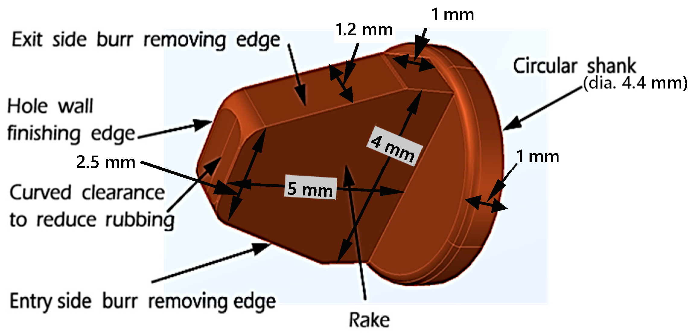
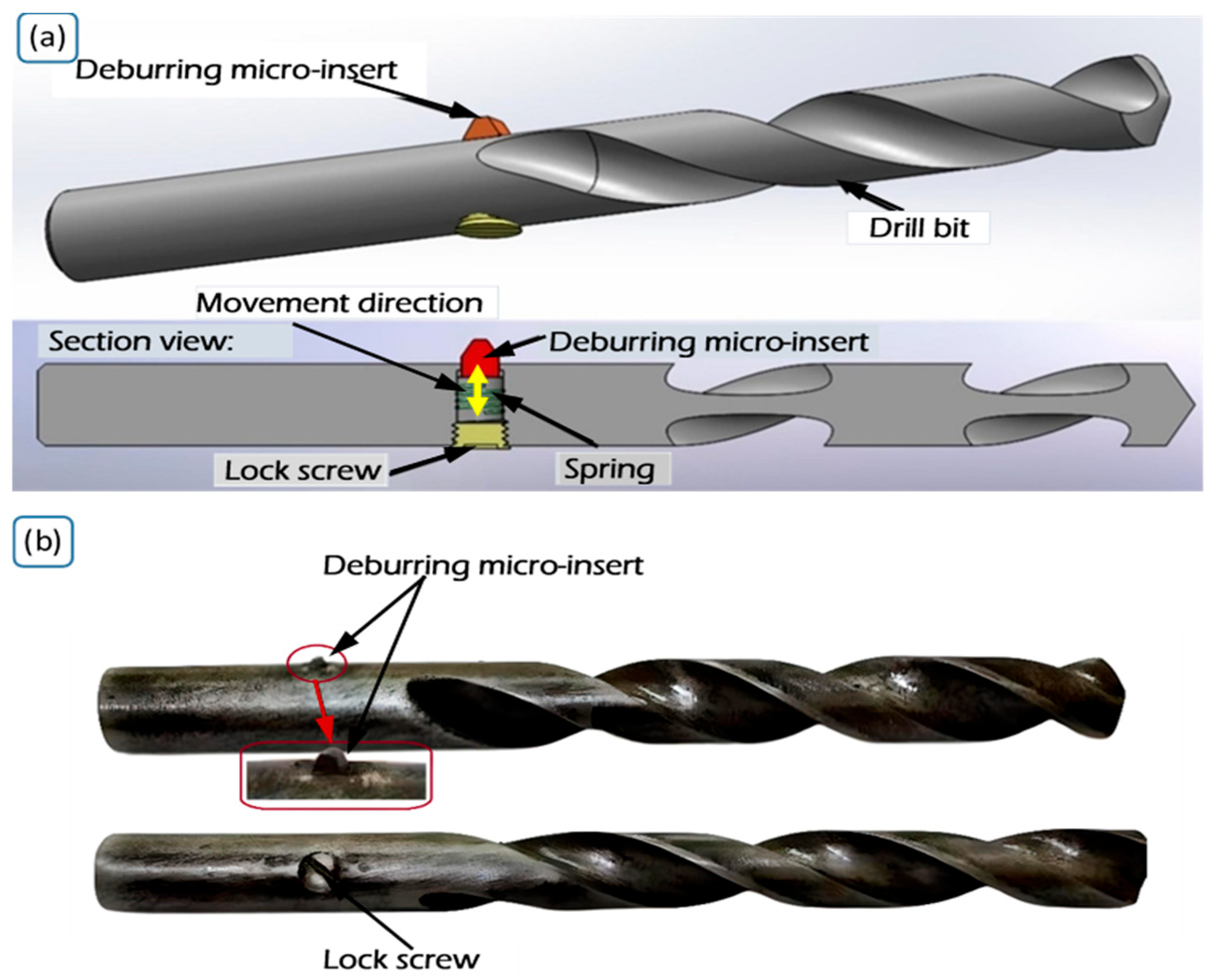
2.1. Modified-1: With a Deburring Micro-Insert Fitted Inside the Twist Drill Bit

The designed deburring micro-insert comprises two key components: a wedge-shaped head at the top and a circular bottom section designed to house a spring. Both cutting edges have equal lengths, ensuring uniform deburring. A curved portion, with multiple curvatures, follows the cutting edges to prevent hole enlargement during operation. The CAD model of the deburring tool is shown in Figure 1.

To attach the deburring micro-insert to the drill, it is inserted into the shank drilled hole and pressed with a spring, which is further fixed by a small screw to ensure flexible in–out movement during operation, as presented in Figure 2a.

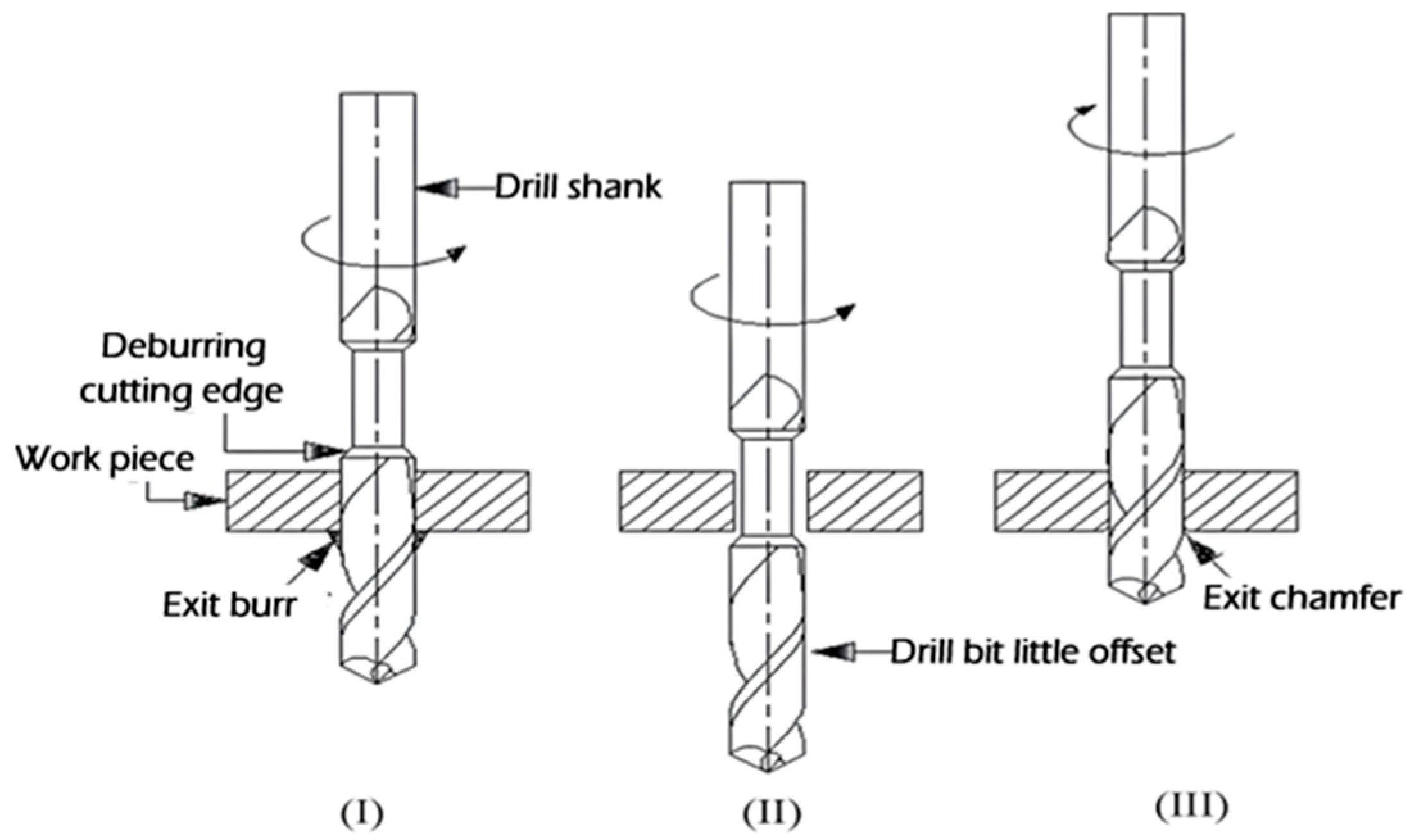
Working Principle of Modified-1 Drill Bit with Deburring Micro-Insert

As the drill feed advances, the deburring micro-insert’s entry-side edge removes the entry burr, while its inclined head edge guides its entry into the cavity. The curved nose prevents excessive hole widening while refining the hole wall under spring action. During exit and return drilling, the deburring micro-insert repeats the actions, removing exit burrs and forming chamfers on both sides (Figure 3). This process ensures efficient burr removal at both entry and exit points.

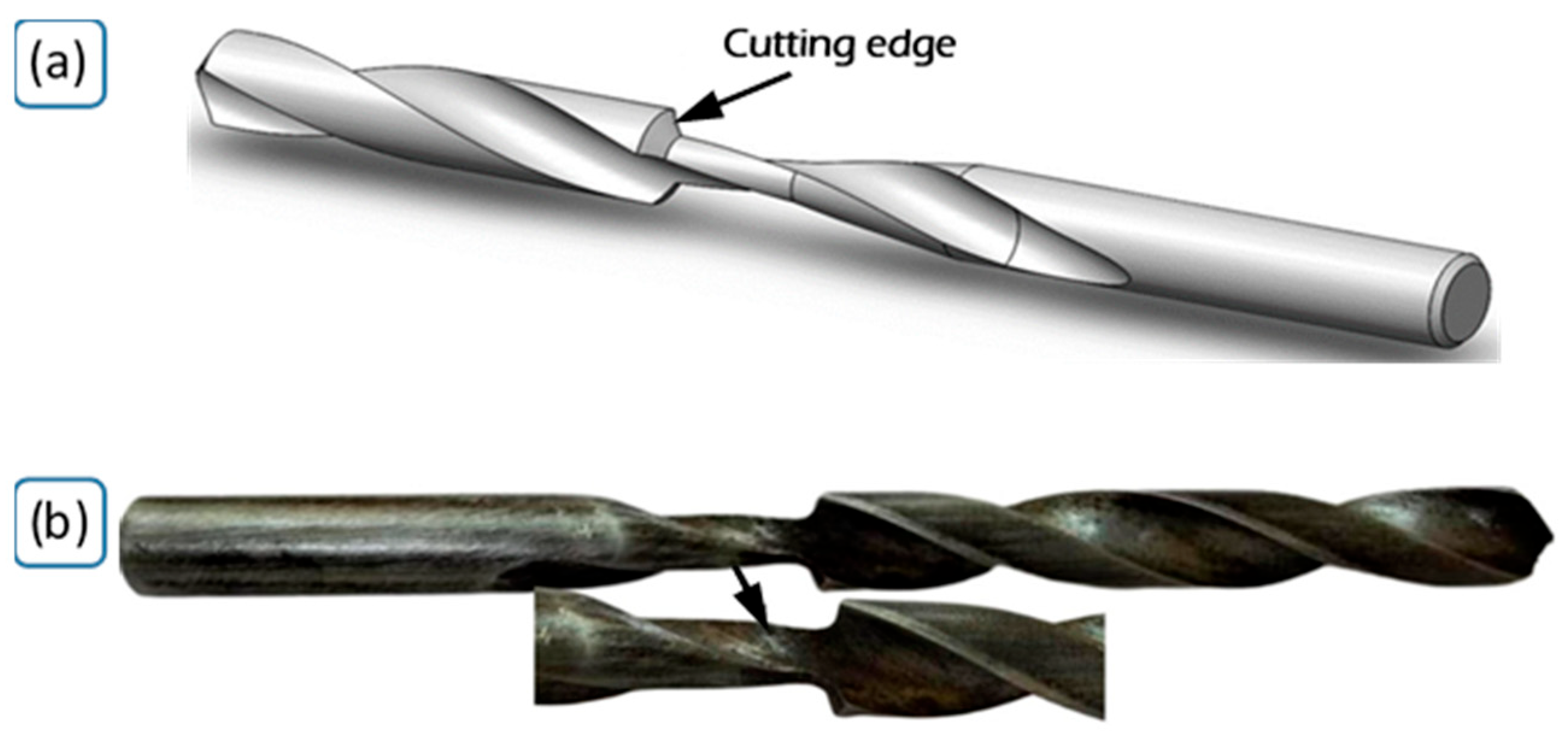
2.2. Modified-2: Drill Bit with Additional Cutting Edge

The second drill bit modification introduces an additional cutting edge opposite the tip’s cutting edge to enhance the deburring efficiency. This is achieved using a grinding machine while ensuring proper fixation. The modification was applied after the shank position, as depicted in Figure 4.

Working Principle of Modified-2 Drill Bit

As the Modified-2 drill bit advances, its cutting edge exits the workpiece. During retraction, the opposite cutting edge reaches the exit, and a slight positional adjustment ensures proper contact with the exit-side burr. The drill then performs one rotation along the hole perimeter, effectively removing the burr and forming a chamfer. This process, optimized via CNC control, is driven by the drill’s backward feed motion and cutting-edge geometry. The drilling and deburring sequence is shown in Figure 5.

2.3. Experimental Details

A schematic presentation of the experimental method is given in Figure 6.

Drilling experiments were conducted using a radial drill machine (Pathak Industries, Model 40R/38P, Howrah, India) with standard drill bits and the Modified-1 and Modified-2 drill bits. Tests were conducted at varying spindle speeds under three conditions: dry, wet with water, and wet with kerosene. The machine, equipped with an auto-feed mechanism, enabled controlled forward and backward feeds. Maintaining a constant feed rate of 0.2 mm/rev throughout the experiment facilitated a controlled analysis by isolating the influence of other factors and ensuring reliable data interpretation. Drilling was performed on a 10-mm-thick aluminum plate (100 mm × 50 mm × 10 mm), with its chemical composition and mechanical properties detailed in

Table 1. Composition of aluminum 6061-T6 (% wt).

Element	Mg	Si	Fe	Cu	Cr	Zn	Ti	Mn	Others	Al
Amount (% wt)	0.80–1.20	0.40–0.80	0.0–0.70	0.15–0.40	0.04–0.35	0.0–0.25	0.0–0.15	0.0–0.15	0.0–0.15	Balance

and

Table 2. Mechanical properties of aluminum 6061-T6.

Property	Density	Modulus of Elasticity	Poisson’s Ratio	Melting Point	Thermal Conductivity	Thermal Expansion Coefficient	Proof Stress	Tensile Strength	Shear Strength	Brinell Hardness
Value	2.70 g/cm3	70 GPa	0.33	650 °C	166 W/m.K	23.6 × 10−6/K	240 MPa	260 MPa	180 MPa	95

. Figure 7 displays a photograph of the workpieces after the drilling process with the normal and modified drills.

2.3.1. Design Parameters with Their Levels

The spindle speeds, drill types, and environmental conditions were chosen as input parameters, each with three distinct levels. Using a full factorial design approach, 27 experimental runs were conducted. A detailed summary of the experimental parameters and their respective levels is presented in

Table 3. Levels of control parameters for the experiment.

	Level
Parameters	−1	0	+1
Speed (rpm)	1000	2000	3000
Drill type	Normal twist drill	Modified-1	Modified-2
Environmental condition	Dry	Water	Kerosene

.

2.3.2. Measurement Methods

During each drilling operation, the temperature was monitored using an infrared thermometer (−50 °C to 500 °C), precisely aimed at the cutting zone to record real-time fluctuations. The peak temperature was recorded as the drilling temperature. The spindle speed was adjusted by repositioning the belt on pulleys of different diameters and measured using a digital tachometer. Instrument specifications are listed in

Table 4. Measuring instrument details.

Parameter	Measuring Instrument	Specifications
Burr Height	Vision Measuring Machine	Maker: Mitutoyo Model: Quick Scope—l2010Z/AFC XYZ measuring volume: 200 × 100 × 150 mm Resolution: 0.1 pm
Temperature	Infrared thermometer	Model no.: HTC MTX-1 Temperature range: −50 °C to 500 °C Accuracy: −20 °C to 0 °C/−4 °F
Spindle Speed	Digital tachometer	Model no.: DT—2235B Speed range: 5 to 19,999 RPM
Surface Roughness	Taly Surf	Mitutoyo SurfTest SJ-210, Kawasaki, Japan

.

The four values of the average surface roughness of each drilled hole were measured using the Mitutoyo SurfTest SJ-210 surface roughness tester, manufactured in Japan.

2.4. Multi-Response Optimization

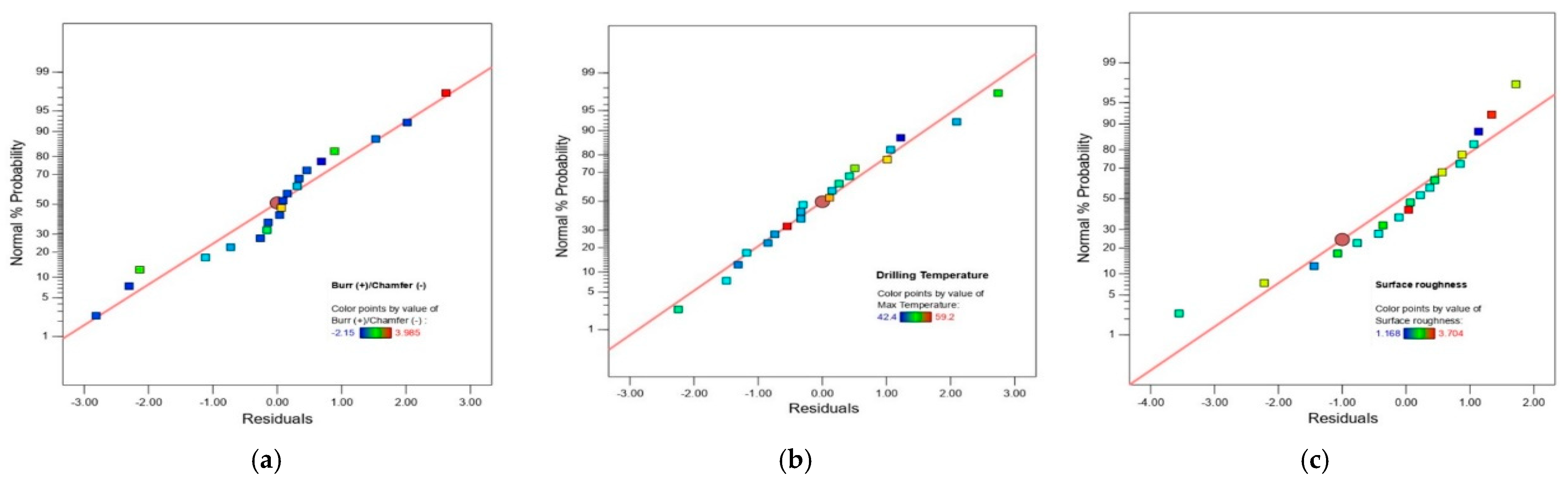
2.4.1. Response Surface Methodology

A comprehensive set of 27 experimental runs was executed, encompassing all possible combinations of the selected input parameters based on a full factorial design. To enhance the reliability of the data, each experiment was performed in triplicate, and the mean value was used for further analysis. The final experimental results, derived from this design approach, are summarized in

Table 5. Experimental input parameters and respective responses.

SL No.	Drill Type	Spindle Speed (rpm)	Environmental Condition	Burr (+)/Chamfer (−) Height (mm) (Z1)	Drilling Temperature (°C) (Z2)	Surface Roughness (µm) (Z3)
1	Normal	1000	Dry	3.985	59.2	3.624
2	Normal	1000	Water	2.745	44	3.218
3	Normal	1000	Kerosene	2.685	48.2	2.941
4	Normal	2000	Dry	2.790	58.5	3.015
5	Normal	2000	Water	1.630	47.7	2.981
6	Normal	2000	Kerosene	1.600	52.3	2.644
7	Normal	3000	Dry	1.520	55.4	2.575
8	Normal	3000	Water	0.497	41.7	2.683
9	Normal	3000	Kerosene	0.456	46.5	2.240
10	Modified-1	1000	Dry	−1.250	57.8	0.917
11	Modified-1	1000	Water	−1.260	45.9	0.746
12	Modified-1	1000	Kerosene	−1.280	50.9	0.106
13	Modified-1	2000	Dry	−1.720	56.4	0.734
14	Modified-1	2000	Water	−1.750	45.5	0.506
15	Modified-1	2000	Kerosene	−1.780	52.1	0.084
16	Modified-1	3000	Dry	−2.100	49.8	0.512
17	Modified-1	3000	Water	−2.150	42.4	0.338
18	Modified-1	3000	Kerosene	−2.180	47.4	0.082
19	Modified-2	1000	Dry	−0.950	53.5	3.704
20	Modified-2	1000	Water	−1.100	45.4	3.418
21	Modified-2	1000	Kerosene	−1.120	48.5	3.013
22	Modified-2	2000	Dry	−1.450	55.8	2.843
23	Modified-2	2000	Water	−1.480	45.4	3.002
24	Modified-2	2000	Kerosene	−1.500	51.8	2.753
25	Modified-2	3000	Dry	−1.810	46.4	2.319
26	Modified-2	3000	Water	−1.870	40.3	2.219
27	Modified-2	3000	Kerosene	−1.890	46.6	1.948

. The relationship between the response variables and the corresponding input parameters (mᵢ) was modeled through regression analysis, as outlined in Equation (1), following the principles of the Design of Experiments (DoE):

$$Z=f\left(m_1,m_2,........,m_k\right)\pm residual error$$

(1)

where f represents a response function. The second-order response surface model is expressed as follows:

$$Z={\alpha }_0+{\sum }_{i=1}^n{\alpha }_i{m}_i+{\sum }_{i=1}^n{\alpha }_{ii}{m}_i^2+{\sum }_i^n{\sum }_j^n{\alpha }_{ij(i<j)}{m}_i{m}_j\pm \epsilon$$

(2)

where, ${\alpha }_0$, ${\alpha }_i$, ${\alpha }_{ii}$, and ${\alpha }_{ij}$ are regression coefficients. The analysis of the output response (burr (+)/chamfer (−) height, drilling temperature, and surface roughness) performance was carried out using the Design Expert (v13) software.

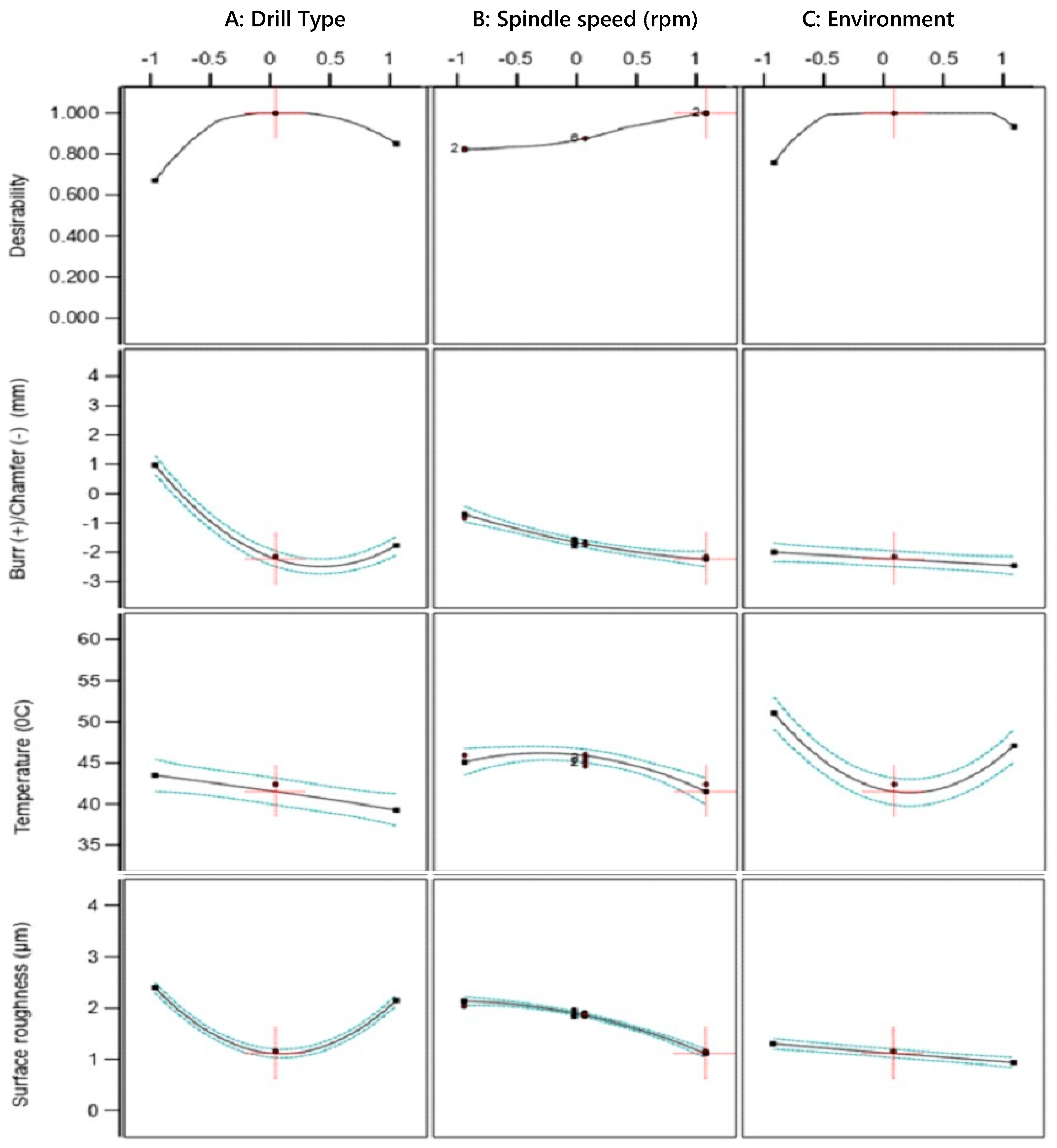
2.4.2. Desirability Function Analysis

Desirability function analysis (DFA) was used to optimize the drilling process parameters—drill type, spindle speed, and environmental conditions—by minimizing the burr/chamfer height, drilling temperature, and surface roughness. Each response was converted into a desirability value (0 to 1), and the geometric mean of these values formed an overall desirability index, which was maximized to identify the optimal machining conditions for improved drilling quality.

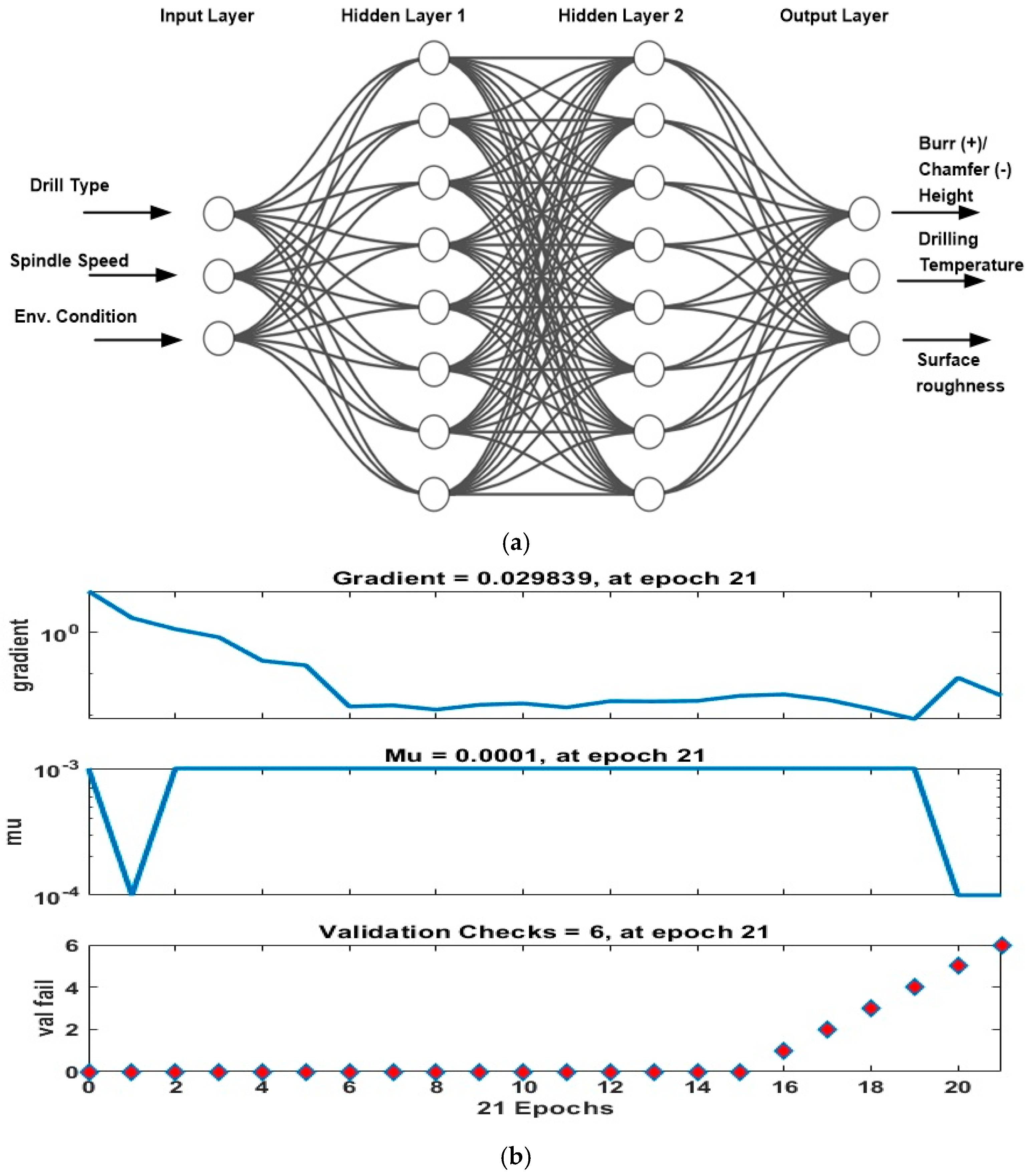
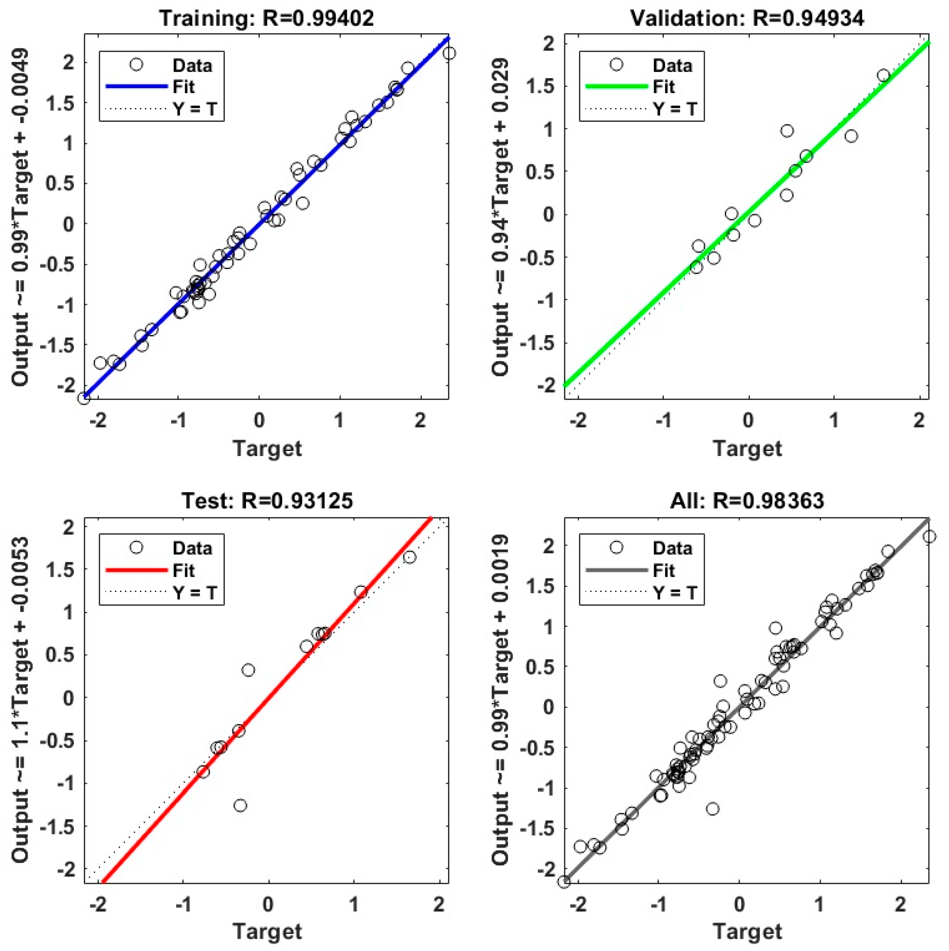
2.4.3. Artificial Neural Networks

Artificial neural networks (ANNs) are computational models designed to capture complex relationships between inputs and outputs using interconnected layers of neurons. In this study, an ANN was developed to predict the burr/chamfer height, drilling temperature, and surface roughness based on the drill type, spindle speed, and environ-mental conditions. The model was trained using 70% of the dataset, with 15% each for testing and validation, employing the Levenberg–Marquardt (LM) algorithm to minimize prediction errors. Performance was evaluated using metrics such as the mean squared error (MSE), root mean squared error (RMSE), and correlation coefficients (R2). MATLAB R2016a was used for model development and performance assessment, with the MSE and mean absolute percentage error (MAPE) used to quantify the training and testing accuracy, respectively, as described in Equations (3) and (4):

$$MSE={\displaystyle \frac{1}{N}}{\displaystyle \sum _{n=1}^N{(Actual-\mathrm{Pr}edicted)}^2}$$

(3)

$$MAPE={\displaystyle \frac{1}{N}}{\displaystyle \sum _{n=1}^N\frac{\left|Actual-\mathrm{Pr}edicted\right|}{Actual}}\times 100$$

(4)

2.4.4. MOGA Analysis

In this study, Multi-Objective Genetic Algorithm (MOGA) analysis is employed to optimize the drilling parameters, considering the drill type, spindle speed, and environmental conditions as input factors, to minimize the burr height (positive)/chamfer height (negative), drilling temperature, and surface roughness. MOGA is an evolutionary optimization technique based on the principles of natural selection and genetic evolution, making it well suited for solving complex multi-objective problems where trade-offs between multiple conflicting responses must be considered. MOGA operates by generating an initial population of solutions and evolving them through iterative processes, including selection, crossover, and mutation. The algorithm evaluates each solution using a fitness function; in this work, it was designed to minimize all three drilling responses. Through multiple generations, MOGA identifies a set of optimal solutions known as the Pareto front, where no single solution can be improved without compromising at least one objective. The final optimal drilling parameters were selected from this Pareto-optimal set based on the best trade-off among the burr height, drilling temperature, and surface roughness. The procedural steps involved in the MOGA-ANN approach are illustrated in Figure 8.

To minimize the objective functions z₁, z₂, and z₃, the developed ANN model was utilized within the MOGA-ANN optimization process, aiming to identify the most suitable input variable set under the following criteria.

Objectives:

• z₁ = min (burr height (positive)/chamfer height (negative));
• z₂ = min (drilling temperature);
• z₃ = min (surface roughness).

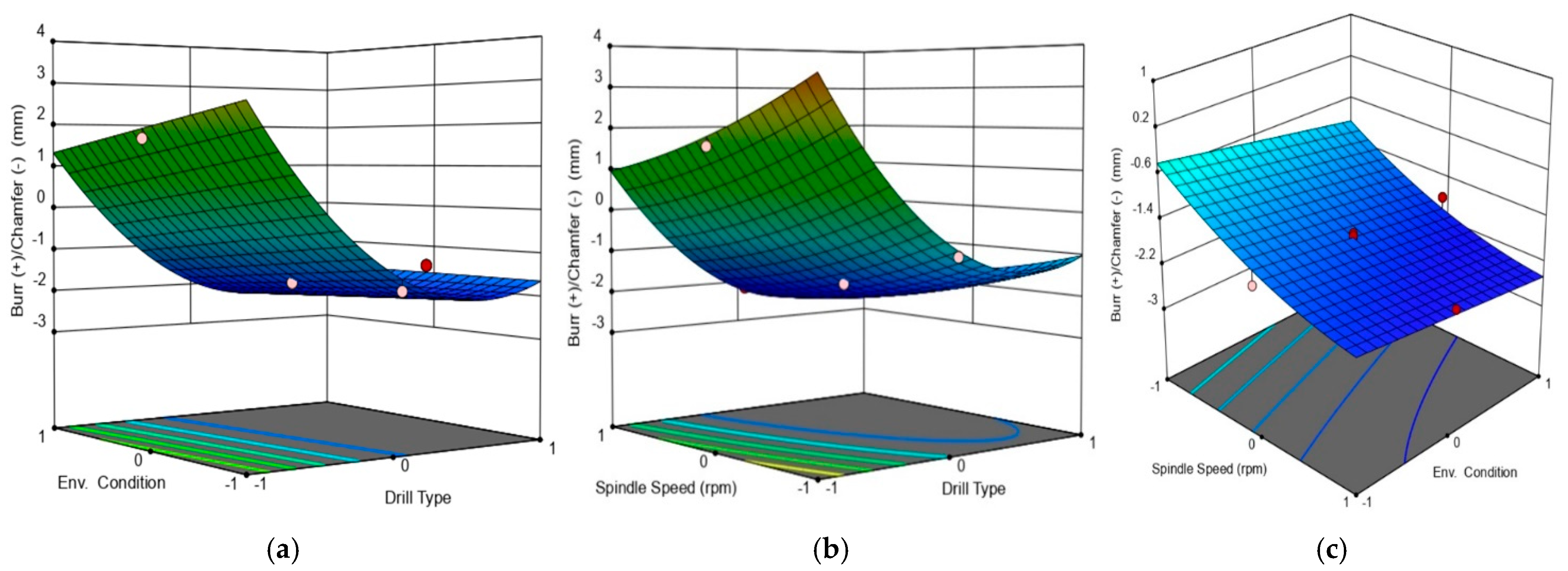
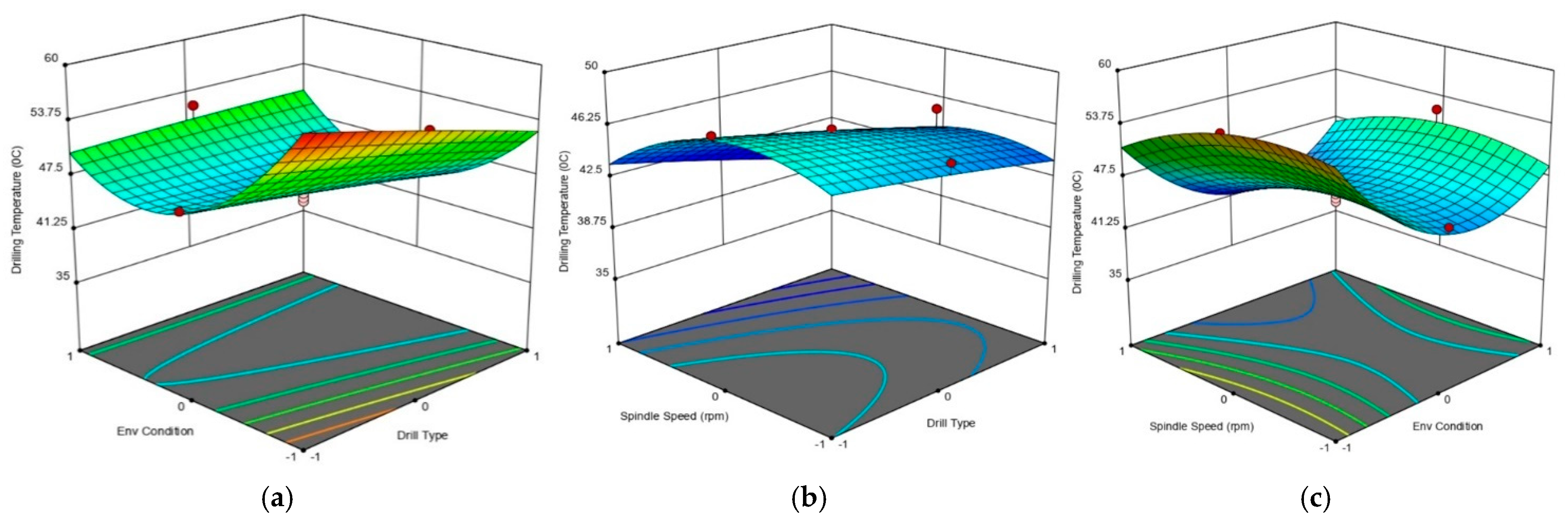
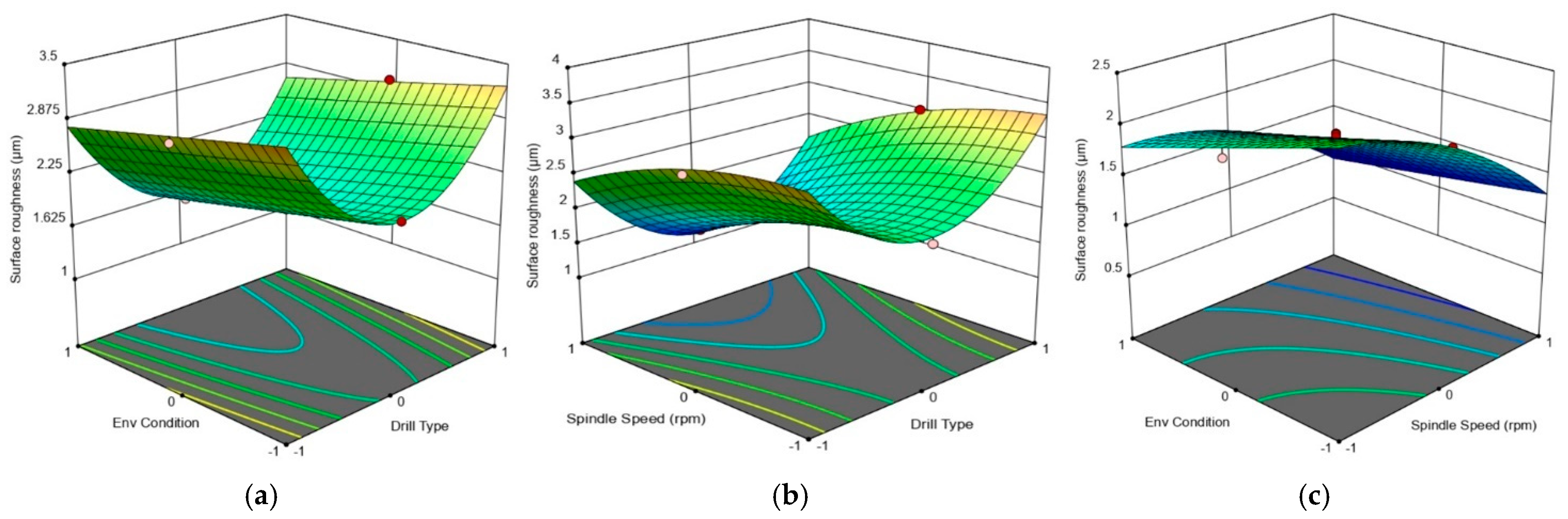
3. Results and Discussion

Mathematical modeling using regression analysis is an effective approach to understanding and quantifying the relationships between input parameters and output responses. In this study, regression analysis is applied to establish a predictive model for the burr height (positive)/chamfer height (negative), drilling temperature, and surface roughness, considering the drill type, spindle speed, and environmental conditions as input parameters. A summary of the model fit for each output response is provided in

Table 6. Fit summary statistics.

Source	Burr (+)/Chamfer (−) Height		Drilling Temperature		Surface Roughness
	F-Value	p-Value	F-Value	p-Value	F-Value	p-Value
Linear vs. Mean	9.12	0.0009	3.11	0.0560	3.21	0.0514
2FI vs. Linear	0.3772	0.7710	0.7554	0.5387	0.0944	0.9618
Quadratic vs. 2FI	229.63	<0.0001	61.00	<0.0001	599.59	<0.0001
Cubic vs. Quadratic	25.52	0.0007	0.6406	0.6530	2.92	0.1166

, while the normal probability plots of the residuals associated with these responses are illustrated in Figure 9a–c. To ensure an accurate and reliable model, the highest-order polynomial is selected based on a lack of fit and statistical significance. In this study, the quadratic regression model is chosen for all three responses, as the lack of fit test indicates non-significance, confirming a good fit to the experimental data. A backward elimination process is employed to remove statistically insignificant terms (highlighted terms in Table 4), ensuring a simplified and effective model.

Table 7. ANOVA results.

Source	Burr (+)/Chamfer (−) Height		Drilling Temperature		Surface Roughness
	F-Value	p-Value	F-Value	p-Value	F-Value	p-Value
Model	227.58	<0.0001	38.75	<0.0001	327.70	<0.0001
A—Drill Type	1070.56	<0.0001	25.27	0.0005	34.73	0.0048
B—Spindle Speed	203.01	<0.0001	29.71	0.0003	866.75	<0.0001
C—Environmental Condition	24.92	0.0005	77.11	<0.0001	239.62	<0.0001
AB	40.90	<0.0001	1.40	0.2635	20.59	0.0011
AC	19.47	0.0013	26.13	0.0005	0.0813	0.7813
BC	0.4630	0.5117	6.11	0.0330	18.75	0.0015
A2	319.29	<0.0001	0.0438	0.8384	1232.53	<0.0001
B2	6.19	0.0321	16.16	0.0024	48.80	<0.0001
C2	3.168 × 10−6	0.9986	144.42	<0.0001	0.0046	0.9473
Lack of Fit	4.51	0.2303	5.08	0.6581	2.84	0.1221
	Not significant		Not significant		Not significant
R2	0.9951		0.9721		0.9966
Adj R2	0.9908		0.9470		0.9936

provides the ANOVA results, including the adjusted and predicted R² values, F-values, and p-values for each response, offering insights into model significance and adequacy. The statistical evaluation ensures that the developed regression model effectively represents the relationships between the machining parameters and response variables, making it a valuable tool for process optimization.

The following equations represent the response models, where the input parameters are expressed as coded factors:

$$Z_1=-1.776-1.726A-0.717B-0.252C+1.878A^2+0.065B^2+0.378AB+0.085CA$$

(5)

$$Z_2=46.859-1.1A-2.05B-2.69C-3.39B^2+7.805C^2+1.44BC+0.98CA$$

(6)

$$Z_3=1.9214-0.047A-0.603B-0.229C+1.036A^2+0.036B^2-0.084AB+0.003BC$$

(7)

Figure 10a shows that the burr height is the highest in dry conditions and with conventional drills, due to increased friction and plastic deformation at the hole exit. As the lubrication improves (water/kerosene) and modified drills are used, the burr height decreases, leading to possible chamfer formation due to better chip evacuation and reduced tool wear. Figure 10b indicates that higher burr formation occurs at lower spindle speeds, particularly with conventional drills, due to poor shearing and increased plastic deformation. Increasing the spindle speed and using modified drills significantly reduces the burr height and can lead to chamfering, as higher speeds enhance material shearing and chip removal. Figure 10c confirms that higher spindle speeds and effective cooling minimize burr formation and promote chamfering, as improved cutting conditions reduce adhesion and plastic deformation. The contour plots in all figures highlight that the best hole quality is achieved with an optimized spindle speed, drill type, and lubrication, reducing the post-processing needs.

The graph (Figure 11a) illustrates the variations in the drilling temperature during the drilling of aluminum 6061-T6 as influenced by the environmental conditions and drill type. The z-axis represents the drilling temperature, while the x-axis corresponds to the environmental conditions (dry, water, and kerosene), and the y-axis represents the drill type (normal, Modified-1, and Modified-2). The plot shows that the temperature is the highest in dry conditions with conventional drill types, as indicated by the red-colored upper surface. This is due to the absence of lubrication, which leads to higher friction, excessive heat generation, and poor heat dissipation. Conversely, the temperature decreases significantly with effective cooling (water or kerosene) and an optimized drill geometry, as seen in the lower green–blue region. The downward curvature of the surface suggests that coolants and modified drill designs help in reducing heat buildup, improving the tool life, and enhancing the drilling performance. Figure 11b shows that the temperature is relatively higher at lower spindle speeds, especially with conventional drills, due to prolonged tool–material contact, leading to more heat buildup. However, the temperature decreases as the spindle speed increases and when modified drills are used, as seen in the lower blue region. This reduction occurs because higher spindle speeds improve chip evacuation and reduce frictional heat, while optimized drill designs enhance the cooling efficiency and minimize heat generation. Figure 11c illustrates the effects of the spindle speed and environmental conditions on the drilling temperature during drilling. Higher temperatures are observed under dry conditions and lower spindle speeds due to increased friction and heat accumulation. In contrast, improved lubrication (moving towards water or kerosene cooling) and higher spindle speeds reduce the temperature, as coolants enhance heat dissipation and minimize tool–workpiece friction.

From Figure 12a, higher surface roughness is observed in dry conditions and with conventional drills, as seen in the upper region of the plot. This occurs due to increased friction, heat generation, and poor chip evacuation, leading to tool wear and surface damage. As the lubrication improves, particularly with water or kerosene cooling, and when the Modified-1 drill is used, the surface roughness decreases. This is evident from the lower region of the surface plot. The presence of a coolant helps to reduce heat and friction during drilling, leading to a better surface finish. Additionally, the optimized geometry of the Modified-1 drill enhances chip evacuation, preventing excessive tool wear and surface damage, resulting in a smoother hole. Figure 12b shows the effects of the spindle speed and drill type on the surface roughness. At lower spindle speeds, the surface roughness is higher with conventional drills, but it decreases when using the Modified-1 drill, likely due to better chip evacuation and reduced tool wear. However, at higher spindle speeds, the surface roughness increases again, possibly due to excessive heat generation and poor chip control, which negatively impact the surface finish. Figure 12c illustrates the combined effects of the spindle speed and environmental conditions on the surface roughness. The surface roughness remains relatively low across all conditions, with slight variations based on lubrication and cooling. As the lubrication improves (moving towards water or kerosene cooling), the surface roughness slightly decreases, likely due to reduced heat generation and better chip evacuation, which enhance the surface finish.

The perturbation plots in Figure 13a–c illustrate the relative impacts of key process parameters on the three responses in the drilling operation. Figure 13a shows the effects of the drill type (A), spindle speed (B), and environmental conditions (C) on the burr height. The drill type (A) has the most significant influence, with higher burr formation with a normal drill and chamfer formation with modified tools. The spindle speed (B) and environmental conditions (C) have a comparatively weaker effect, mainly contributing to a gradual reduction in burr height. The next perturbation plot (Figure 13b) shows the influence of the process parameters on the temperature during drilling. Among the three parameters, the environmental condition (C) has the most significant impact, as indicated by its pronounced curvature. The spindle speed (B) and drill type (A) have a relatively weaker effect, with the spindle speed slightly reducing the temperature. Figure 13c illustrates the effects of the drill type (A), spindle speed (B), and environmental conditions (C) on the surface roughness.

The drill type (A) has the most significant influence, showing a parabolic trend where the surface roughness increases at both extremes. The spindle speed (B) has a negative correlation, indicating that higher spindle speeds reduce the surface roughness, while the environmental condition (C) has a minimal effect.

Figure 14a–c present a comparison between the experimental and predicted values of all responses across different experimental runs. The close alignment between the experimental and predicted values indicates that all models effectively represent the variation in each response value across different runs.

Figure 15 presents the optimized drilling results obtained using the desirability function, which forecasted a minimum chamfer height of −2.066 mm, a drilling temperature of 42.19 °C, and surface roughness of 1.514 µm. With a composite desirability value of 0.976, the optimization process is considered successful, as the value is close to the maximum desirable limit of 1. The optimized performance outcomes are evaluated for Modified-1 operating at 3000 rpm in a water environment, as these conditions were identified as the optimal settings through the analysis.

To enhance the analytical process, an artificial neural network (ANN) has been implemented, and its structural layout is presented in Figure 16a. This ANN model predicts the drilling performance based on three input parameters: the drill type, spindle speed, and environmental conditions. It consists of two hidden layers that process the inputs through interconnected neurons, applying activation functions to learn patterns. The output layer provides predicted values for the burr height (positive) or chamfer height (negative), drilling temperature, and surface roughness. By adjusting the connection weights, the ANN identifies relationships between the input and output parameters, making it useful in optimizing the drilling conditions. Figure 16b represents the training performance of the artificial neural network (ANN) over 21 epochs. The top graph shows the gradient, which decreases initially but stabilizes later, indicating convergence. The middle graph represents the learning rate parameter (Mu), which remains at 0.0001 for most epochs but drops towards the end, suggesting adaptive tuning. The bottom graph shows validation checks, increasing steadily after epoch 10 and reaching six at epoch 21, indicating early stopping to prevent overfitting. This suggests that the training process was halted at an optimal point to maintain generalization.

The LM backpropagation algorithm, known for its effectiveness in supervised learning, is utilized to maximize the R² value, as demonstrated in Figure 17. This figure represents the regression analysis of the artificial neural network (ANN) model, showing the correlation between the predicted and actual target values for the training, validation, testing, and overall data. The R values (correlation coefficients) indicate how well the model fits the data: training (R = 0.99402), validation (R = 0.94934), test (R = 0.93125), and overall (R = 0.98363). A value close to 1 suggests a strong linear relationship and good predictive performance. The regression equations show the fitted line’s slope and intercept, with the training and overall datasets exhibiting a nearly perfect fit. However, the test data have a slightly weaker correlation (R = 0.93125), indicating some potential generalization issues. Overall, the model performs well, but minor overfitting may be present. Figure 18a graphically depicts the distribution of the residual errors, offering a concise assessment of the model performance. This error histogram represents the distribution of the errors (differences between target and predicted outputs) for the training, validation, and test datasets in the artificial neural network (ANN) model. The x-axis represents the error values, while the y-axis indicates the number of instances for each error range. The blue bars represent training errors, the green bars represent validation errors, and the red bars correspond to test errors. The orange line at zero indicates the ideal case where the predictions perfectly match the targets. The histogram shows a normal-like distribution, with most errors concentrated around zero, indicating that the model has good predictive accuracy. Figure 18b signifies the training performance of the artificial neural network by plotting the mean squared error (MSE) against the number of epochs for the training (blue), validation (green), and test (red) datasets. The best validation performance is achieved at epoch 15 with an MSE of 0.044708, as marked by the green circle. Initially, all errors decrease, indicating learning progress, but, after epoch 15, the validation and test errors start increasing, while the training error continues decreasing. This suggests overfitting, meaning that the model learns the training data well but loses its generalization capability. Early stopping at epoch 15 prevents further overfitting and ensures better generalization.

Using both the RSM and MOGA-ANN for comparison in multi-objective optimization provides a comprehensive approach to addressing complex optimization problems. The results of the MOGA optimization, detailing the optimal input settings and their associated output responses, are summarized in

Table 8. Optimized values (MOGA-ANN).

SL No.	Input Parameter			Output
	Drill Type	Spindle Speed (rpm)	Environmental Condition	Burr (+)/Chamfer (−) Height (mm)	Drilling Temperature (°C)	Surface Roughness (µm)
1	Modified-1	3000	Kerosene	−2.252	47.88	0.081
2	Modified-1	3000	Water	−2.611	40.76	0.187
3	Modified-2	3000	Water	−1.916	40.28	2.236
4	Modified-2	3000	Water	−2.001	40.34	2.131
5	Modified-1	3000	Water	−2.673	40.88	0.291
6	Modified-1	3000	Water	−2.012	42.25	0.113
7	Modified-2	3000	Water	−2.268	40.47	1.939
8	Modified-1	3000	Kerosene	−2.829	45.77	0.182
9	Modified-1	3000	Water	−2.339	40.51	0.374
10	Modified-1	3000	Water	−2.448	40.59	0.270
11	Modified-1	3000	Kerosene	−2.809	44.94	0.122
12	Modified-1	3000	Water	−2.510	40.66	0.096
13	Modified-2	3000	Water	−2.001	40.34	2.131
14	Modified-1	3000	Kerosene	−2.816	43.95	0.015
15	Modified-2	3000	Water	−2.321	40.50	1.891
16	Modified-2	3000	Water	−1.977	40.31	2.188
17	Modified-1	3000	Kerosene	−1.910	46.66	0.311
18	Modified-1	3000	Water	−2.540	40.68	0.173

. Figure 19 displays the Pareto front for the three output objectives—the burr (+)/chamfer (−) height, drilling temperature, and surface roughness—highlighting the trade-offs among these competing responses.

The MOGA-ANN approach is employed to optimize the input parameters. The optimized parameter sets derived from this method are subsequently used to perform confirmatory experiments aimed at validating the model’s predictive accuracy. The optimal results generated by the MOGA-ANN are presented in Table 8. Confirmatory experiments are conducted, with each experiment repeated three times. The average of the results is calculated to ensure accuracy and consistency. The results of these validation tests are summarized in

Table 9. Confirmatory study results.

SL No.	Input Parameter			Output
	Drill Type	Spindle Speed (rpm)	Environmental Condition	Burr (+)/Chamfer (−) Height (mm)			Drilling Temperature (°C)			Surface Roughness (µm)
				MOGA-ANN	Experimental	% Variation	MOGA-ANN	Experimental	% Variation	MOGA-ANN	Experimental	% Variation
1	Modified-1	3000	Kerosene	−2.252	−2.18	<3%	47.88	47.4	<1%	0.081	0.079	<2%
2	Modified-1	3000	Water	−2.611	−2.55	<3%	40.76	42.4	<4%	0.187	0.179	<4%
3	Modified-2	3000	Water	−1.916	−1.87	<2.5%	40.28	40.3	<1%	2.236	2.2	<2%
4	Modified-2	3000	Water	−2.001	−1.89	<6%	40.34	42.6	<5%	2.131	2.031	<5%
5	Modified-1	3000	Water	−2.673	−2.521	<4%	40.88	41.88	<2%	0.291	0.281	<3.5%
6	Modified-1	3000	Water	−2.012	−2	<1%	42.25	43.45	<3%	0.113	0.116	<2%
7	Modified-2	3000	Water	−2.268	−2.168	<5%	40.47	43	<5%	1.939	1.9	<2%
8	Modified-1	3000	Kerosene	−2.829	−2.67	<6%	45.77	44.54	<3%	0.182	0.185	<2%
9	Modified-1	3000	Water	−2.339	−2.39	<2%	40.51	42.01	<3%	0.374	0.37	<2%
10	Modified-1	3000	Water	−2.448	−2.65	<7%	40.59	42.9	<5%	0.27	0.276	<1%
11	Modified-1	3000	Kerosene	−2.809	−2.81	<1%	44.94	43.74	<3%	0.122	0.124	<2%
12	Modified-1	3000	Water	−2.51	−2.42	<4%	40.66	41.95	<3%	0.096	0.093	<2%
13	Modified-2	3000	Water	−2.001	−2.1	<4%	40.34	40.94	<1%	2.131	2.1	<3%
14	Modified-1	3000	Kerosene	−2.816	−2.844	<1%	43.95	42.75	<2%	0.015	0.016	<1%
15	Modified-2	3000	Water	−2.321	−2.301	<1%	40.5	40.35	<2%	1.891	1.88	<1%
16	Modified-2	3000	Water	−1.977	−1.99	<1%	40.31	41.01	<2%	2.188	2.19	<1%
17	Modified-1	3000	Kerosene	−1.91	−1.87	<2%	46.66	45.06	<3%	0.311	0.309	<1%
18	Modified-1	3000	Water	−2.54	−2.643	<4%	40.68	42.01	<3%	0.173	0.175	<1%

. The outcomes reveal a strong correlation between the predicted and experimental values, confirming the reliability of the MOGA-ANN model.

4. Conclusions

In this study, modified drills were developed and experimentally examined with a normal drill in dry, wet, and kerosene conditions. The following findings can be drawn from the current investigation:

• Two modified drill bits were developed for single-pass burr-free drilling, with Modified-1 showing superior burr removal and chamfering performance.
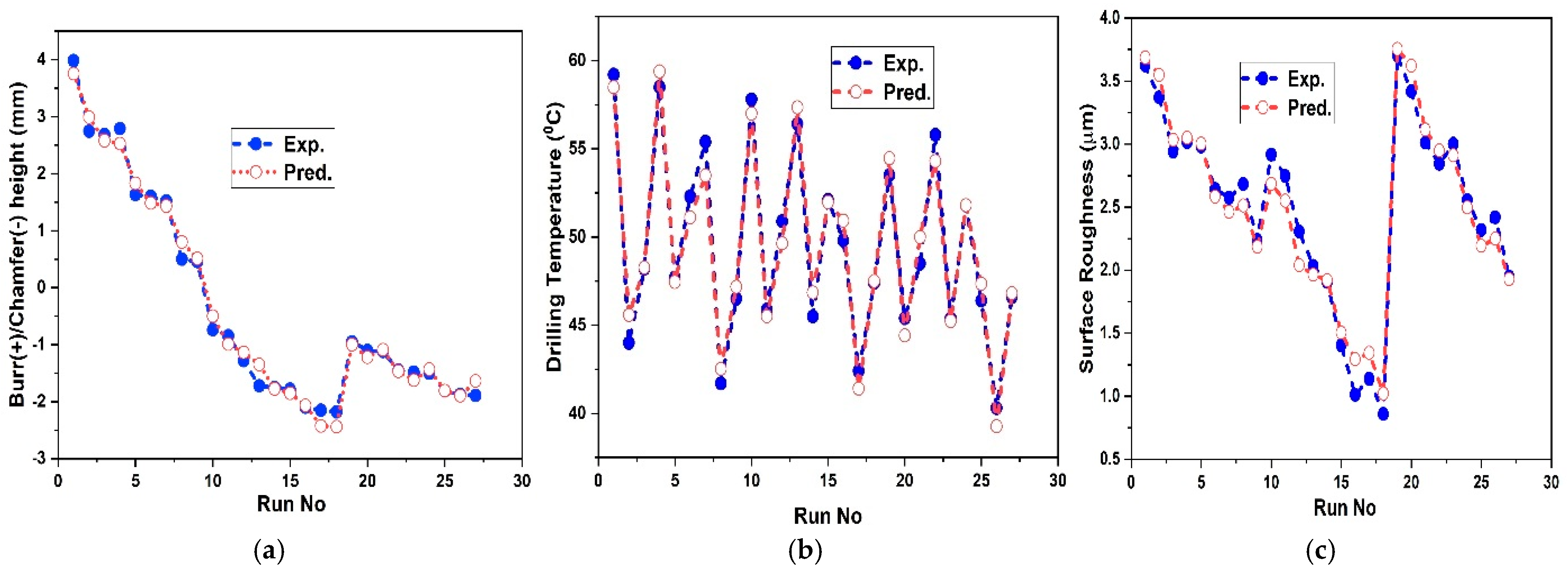
• The RSM and MOGA-ANN effectively modeled and optimized the drilling process, offering reliable predictions of multiple responses.
• Optimal parameters were identified as the use of Modified-1, 3000 rpm, and a water environment, achieving minimal chamfer heights (−2.066 mm), low drilling temperatures (42.19 °C), and an excellent surface finish (1.514 µm).
• Typically, a superior surface finish with roughness as low as 0.016 µm can be achieved under a kerosene-based environment as compared to dry and wet conditions.
• The experimental results matched the MOGA-ANN predictions, with deviations under 6%, validating the model’s accuracy.
• This approach demonstrates the novel integration of tool design and AI optimization, enhancing productivity, reducing post-processing, and improving drilling quality.

Recommendations: The Modified-1 drill type, with a burr removal micro-insert, can be used for single-step drilling, enabling both burr removal and improved finishing of the drilled hole wall surface. The Modified-2 drill bit, which includes an additional cutting edge, is easier to fabricate and thus presents a more cost-effective option for industrial applications focused solely on burr removal, where the surface finish is not essential.

References

1. Dey, B.; Mondal, N.; Mondal, S. Experimental Study to Minimize The Burr Formation in Drilling Process With Artifical Neural Networks (ANN) Analysis. In IOP Conference Series: Materials Science and Engineering; IOP Publishing: Bristol, UK, 2018; Volume 377, p. 012120. [Google Scholar]
2. Gillespie, L.K. Deburring precision miniature parts. Precis. Eng. 1979, 1, 189–198. [Google Scholar] [CrossRef]
3. Blotter, P.T.; Gillespie, L.K. The formation and properties of machining burrs. J. Manuf. Sci. Eng. 1976, 98, 66–74. [Google Scholar]
4. Kim, J.; Min, S.; Dornfeld, D.A. Optimization and control of drilling burr formation of AISI 304L and AISI 4118 based on drilling burr control charts. Int. J. Mach. Tools Manuf. 2001, 41, 923–936. [Google Scholar] [CrossRef]
5. Min, S.; Dornfeld, D.A.; Kim, J.; Shyu, B. Finite element modeling of burr formation in metal cutting. Mach. Sci. Technol. 2001, 5, 307–322. [Google Scholar] [CrossRef]
6. Mondal, N.; Mandal, M.C.; Dey, B.; Das, S. Genetic algorithm-based drilling burr minimization using adaptive neuro-fuzzy inference system and support vector regression. Proc. Inst. Mech. Eng. Part B J. Eng. Manuf. 2020, 234, 956–968. [Google Scholar] [CrossRef]
7. Mondal, N.; Mandal, S.; Mandal, M.C. FPA based optimization of drilling burr using regression analysis and ANN model. Measurement 2020, 152, 107327. [Google Scholar] [CrossRef]
8. Biermann, D.; Hartmann, H. Reduction of burr formation in drilling using cryogenic process cooling. Procedia CIRP 2012, 3, 85–90. [Google Scholar] [CrossRef]
9. Davim, J.P.; António, C.A.C. Optimisation of cutting conditions in machining of aluminium matrix composites using a numerical and experimental model. J. Mater. Process. Technol. 2001, 12, 78–82. [Google Scholar] [CrossRef]
10. Davim, J.P. Statistical and Computational Techniques in Manufacturing; Springer: Berlin/Heidelberg Germany, 2014. [Google Scholar] [CrossRef]
11. Davim, J.P.; António, C.A.C. Optimal drilling of particulate metal matrix composites based on experimental and numerical procedures. Int. J. Mach. Tools Manuf. 2001, 41, 21–31. [Google Scholar] [CrossRef]
12. Mondal, N.; Mandal, S.; Mandal, C.M.; Das, S.; Haldar, B. ANN-FPA based modelling and optimization of drilling burrs using RSM and GA. In Advance in Manufacturing Process, Intelligent Methods and System in Production Engineering, Proceedings of the GCMM 2021, Liverpool, UK, 7–9 June 2021; Springer: Cham, Switzerland, 2022; pp. 180–195. [Google Scholar] [CrossRef]
13. Gaitonde, N.V.; Karnik, R.S. Minimizing burr size in drilling using artificial neural network (ANN)-particle swarm optimization (PSO) approach. Int. J. Adv. Manuf. Technol. 2012, 23, 1783–1793. [Google Scholar] [CrossRef]
14. Suresh, S.; Rao, P.V.; Prasad, B. Optimization of drilling parameters for burr minimization in aluminum alloys using RSM. J. Manuf. Sci. Eng. 2016, 138, 051005. [Google Scholar]
15. Kumar, S.; Gupta, M.; Sharma, R. Analysis of drilling burr formation using response surface method-ology. Mater. Manuf. Process. 2018, 33, 678–689. [Google Scholar]
16. Saha, S.; Mondal, A.K.; Čep, R.; Joardar, H.; Haldar, B.; Kumar, A.; Alsalah, N.A.; Ataya, S. Multi-response optimization of electrochemical machining parameters for Inconel 718 via RSM and MOGA-ANN. Machines 2024, 12, 335. [Google Scholar] [CrossRef]
17. Kumar, L.; Kumar, K.; Chhabra, D. Experimental investigations of electrical discharge micro-drilling for Mg-alloy and multi-response optimization using MOGA-ANN. CIRP-J. Manuf. Sci. Technol. 2022, 38, 774–786. [Google Scholar] [CrossRef]
18. Sahoo, A.K.; Mohanty, R.R.; Routara, B.C. Hybrid MOGA-ANN approach for tool wear and burr height optimization in drilling. Procedia CIRP 2019, 84, 415–420. [Google Scholar]
19. Singh, H.; Nayak, D.; Ghosh, S. Multi-objective optimization of drilling force and burr formation in composites using MOGA-ANN. Mater. Today Proc. 2020, 45, 2135–2143. [Google Scholar]
20. Dornfeld, D.A.; Kim, J.S.; Dechow, H.; Hewson, J.; Chen, L.J. Drilling burr formation in titanium alloy, Ti-6AI-4V. CIRP Ann. 1999, 48, 73–76. [Google Scholar] [CrossRef]
21. Murthy, K.S.; Rajendran, I.G. Prediction and analysis of multiple quality characteristics in drilling under minimum quantity lubrication. Proc. Inst. Mech. Eng. Part B J. Eng. Manuf. 2012, 226, 1061–1070. [Google Scholar] [CrossRef]
22. Pramanik, A.; Basak, A.K.; Prakash, C.; Shankar, S.; Chattopadhyaya, S. Sustainability in drilling of aluminum alloy. Clean. Mater. 2022, 3, 100048. [Google Scholar] [CrossRef]
23. Heisel, U.; Schaal, M. Burr formation in short hole drilling with minimum quantity lubrication. Prod. Eng. 2009, 3, 157–163. [Google Scholar] [CrossRef]
24. Agrawal, S.M.; Patil, N.G. Effects of Cryogenic Cooling on Burr Height in Drilling of Ceramic Rein-forced Aluminium Matrix Composites. Int. J. Adv. Res. Eng. Technol. 2020, 11, 851–856. [Google Scholar]
25. Govindaraju, N.; Ahmed, L.S.; Kumar, M.P. Experimental investigations on cryogenic cooling in the drilling of AISI 1045 steel. Mater. Manuf. Process. 2014, 29, 1417–1421. [Google Scholar] [CrossRef]
26. Zhu, Z.; Sun, X.; Guo, K.; Sun, J.; Li, J. Recent Advances in Drilling Tool Temperature: A State-of-the-Art Review. Chin. J. Mech. Eng. 2022, 35, 148. [Google Scholar] [CrossRef]
27. Hussein, R.; Sadek, A.; Elbestawi, M.A.; Attia, M.H. Elimination of delamination and burr formation using high-frequency vibration-assisted drilling of hybrid CFRP/Ti6Al4V stacked material. Int. J. Adv. Manuf. Technol. 2019, 105, 859–873. [Google Scholar] [CrossRef]
28. Franczyk, E.; Ślusarczyk, Ł.; Zębala, W. Drilling Burr minimization by changing drill geometry. Materials 2020, 13, 3207. [Google Scholar] [CrossRef]
29. Ko, S.L.; Lee, J.K. Analysis of burr formation in drilling with a new-concept drill. J. Mater. Process. Technol. 2001, 113, 392–398. [Google Scholar] [CrossRef]
30. HuaNa Tools. All You Need to Know About HSS Drill Bits. Available online: https://huanatools.com/introduction-of-high-performance-drill-bits/ (accessed on 11 January 2023).
31. Quality Tools. A-Z guide for Drilling Aluminium. 11 January 2023. Available online: https://qlt.tools/blogs/insights/drilling-aluminium-guide?srsltid=AfmBOoorMDJmBe7syZrGJ7EQ433eRZcyNhW5jxlynuEE-32svZArOjRv (accessed on 11 January 2024).
32. Ramesh, B.; Elayaperumal, A.; Venkatesh, R.; Madhav, S.; Jain, K. Determination of optimum parameter levels for multi-performance characteristics in conventional milling of beryllium copper alloy by using response surface methodology. Int. J. Innov. Res. Sci. Eng. Technol. 2014, 3, 10916–10923. [Google Scholar]
33. Kim, K.H.; Cho, C.H.; Jeon, S.Y.; Lee, K.; Dornfeld, D.A. Drilling and deburring in a single process. Proc. Inst. Mech. Eng. Part B J. Eng. Manuf. 2003, 217, 1327–1331. [Google Scholar] [CrossRef]
34. Kim, K.H.; Park, N.J. A new deburring for intersecting holes. Proc. Inst. Mech. Eng. Part B J. Eng. Manuf. 2005, 219, 865–870. [Google Scholar] [CrossRef]
Figure 1. CAD model of deburring micro-insert.
Lubricants 13 00273 g001
Figure 2. (a) The CAD model and (b) the actual Modified-1 twist drill bit with a deburring micro-insert.
Lubricants 13 00273 g002
Figure 3. The drilling and deburring sequence: (I) the deburring micro-insert approaches the workpiece; (II) the entry burr is removed; (III) the deburring micro-insert retracts; and (IV) the exit burr is removed through reverse feeding.
Lubricants 13 00273 g003
Figure 4. (a) The Modified-2 drill bit CAD model and (b) an inset photograph of the actual modified drill bit.
Lubricants 13 00273 g004
Figure 5. The sequence of drilling and deburring: (I) exit burr formed; (II) drill bit position with minor offset; (III) removal of the exit burr in reverse motion.
Lubricants 13 00273 g005
Figure 6. Single-step drilling experimental method with measurement methods for temperature, burr height, and surface roughness.
Lubricants 13 00273 g006
Figure 7. Photograph of aluminum workpiece after drilling operation using (I) normal drill, (II) Modified-1, and (III) Modified-2. A negative burr height indicates the height of the chamfer, which is created around the circumference of the hole in the case of modified drills.
Lubricants 13 00273 g007
Figure 8. Steps for MOGA optimization.
Lubricants 13 00273 g008
Figure 9. Normal residual plots for (a) burr (+)/chamfer (−) height, (b) drilling temperature, and (c) surface roughness.
Lubricants 13 00273 g009
Figure 10. Surface plots for burr or chamfer height: (a) env. condition vs. drill type, (b) spindle speed vs. drill type, and (c) spindle speed vs. env. condition.
Lubricants 13 00273 g010
Figure 11. Surface plot for drilling temperature: (a) env. condition vs. drill type, (b) spindle speed vs. drill type, and (c) spindle speed vs. env condition.
Lubricants 13 00273 g011
Figure 12. Surface plot for surface roughness: (a) env. condition vs. drill type, (b) spindle speed vs. drill type, and (c) spindle speed vs. env condition.
Lubricants 13 00273 g012
Figure 13. Perturbation plot for (a) burr/chamfer height, (b) drilling temperature, and (c) surface roughness.
Lubricants 13 00273 g013
Figure 14. Validation between experimental and predicted values for (a) burr/chamfer height, (b) drilling temperature, and (c) surface roughness.
Lubricants 13 00273 g014
Figure 15. Multi-optimization using the “desirability function”.
Lubricants 13 00273 g015
Figure 16. ANN model: (a) structure and (b) training state.
Lubricants 13 00273 g016
Figure 17. ANN-trained model for optimal fitness.
Lubricants 13 00273 g017
Figure 18. (a) Histogram and (b) MSE plot for neural network.
Lubricants 13 00273 g018
Figure 19. Pareto front plot for (a) surface roughness vs. chamfer or burr height and (b) surface roughness vs. temperature.
Lubricants 13 00273 g019