Abstract
This paper addresses the unclear bearing force of an RV reducer shaft by establishing a transmission model and analyzing the force situation of each component. Three force models for the crank support bearing, swivel arm bearing, and main bearing are developed. The force variations under different working conditions and the impact of structural parameters on shaft bearing forces are analyzed. Structural optimization is performed using Kriging-NSGA-II to minimize bearing forces. The results show similar load patterns for the bearings, with the force magnitude being ranked in the following order: rotating arm > crank support > main bearing. After optimization, the bearing forces are reduced by 8.26% for the crank support shaft, 10.35% for the rotating arm shaft, and 5.15% for the main shaft.
1. Introduction
RV reducers stand out as important joints for industrial robots in the era of the slow popularization of industrial automation because of their small size, large transmission ratio, high load-bearing capacity, high motion accuracy, and high transmission efficiency [1,2]. However, due to its complex structure, the internal bearing capacity of the shaft, which is the main moving part, is ambiguous, so research on the bearing capacity of RV reducers is imminent [3].
Great resources have been invested in both RV reducers and their bearings. Peng et al. [4] classified the performance indexes from the perspective of the characterization of three physical quantities, namely, the angle, torque, and speed, and they analyzed the influence of system structure error and test principle error on the measurement of basic physical quantities, such as angle and torque, in a bench-type test system; a parametric characterization model for testing the performance indexes of precision reducer transmission was proposed. Yang et al. [5] conducted a study on the nonlinear dynamic characteristics of Cycloid Ball Planetary Transmission (CBPT) under tooth-root-cutting conditions. The results indicate that damping, the rolling radius, and a short amplitude coefficient significantly affect the system’s stability, and parameter optimization is required to suppress chaotic vibrations. Wang et al. [6] studied the dynamic characteristics of transmission errors in RV reducers. The results show that clearance and contact deformation are the main sources of errors, and the mathematical model closely matches the experimental data within the error range. Tie et al. [7] conducted a force analysis on the transmission torque, crankshaft, output shaft, and cycloid wheel of an RV reducer. The number of teeth engaged between the cycloid wheel and the needle wheel was determined, and the contact deformation and meshing force of each tooth during the engagement of the modified tooth profile of the cycloid wheel and needle wheel were calculated. The results indicate that preloading installation ensures the reliability of the support. Olejarczyk et al. [8] conducted a comparative study on the efficiency of different types of bearings in cycloid gearboxes. Huang et al. [9] incorporated the roller convexity parameter into the optimization design of RV bearings for the first time, addressing the edge stress concentration issue of traditional flat-headed rollers. He and Shan [10] developed a transmission error dynamics model and mathematical equations for RV reducers for robots using a dynamical substructure approach. Wu et al. [11] proposed a force calculation method based on multi-body dynamics and used it to study the law of the influence of input speed and load on the bearing force of a rotating arm shaft. Xu and Yang [12] considered the kinetic characteristics of a cylindrical roller bearing in a swivel arm, proposed an analytical method for multi-tooth meshing contact dynamics in a cycloid pinwheel transmission, and established a kinetic model for that cycloid pinwheel transmission. Olejarczyk et al. [8] conducted a comparative study of the efficiency of different types of bearings in a cycloid pinwheel transmission, and the experimental results under different operating conditions showed that the efficiency of needle roller bearings was significantly higher than that of sleeve bearings. Sun et al. [13] analyzed the effect of working clearance on the contact load and contact deformation of deep-groove ball bearings by performing rigidity analysis and flexibility analysis on the constructed model.
The structure of an RV reducer is complex, and research on the structural optimization thereof is ongoing. Guan and Zhang [14] proposed the concept of the “anti-bow profile” for cycloid and needle wheels to improve the force condition of the tooth surface, and they used the combination of “positive equidistant + negative shift” to construct the anti-bow profile. Yu and Xu [15] used MATLAB2016a to optimize the design of a cycloid needle wheel drive. The results showed that after optimization, the volume was reduced by 26.8% while significantly improving the structural compactness and ensuring the performance in terms of contact strength, bending strength, and other factors. Liang et al. [16] optimized a cycloid pinwheel planetary reducer with a genetic algorithm and with volume and transmission efficiency as the objectives, and they performed simulation analysis based on the finite element method. Wang et al. [17] optimized the cycloid needle wheel planetary reducer using an improved genetic algorithm, with the objectives of minimizing the volume, crankshaft bearing stress, and maximum bending stress of the pins, and they obtained a near-optimal solution.
Although the above-mentioned scholars have studied various components of RV reducers, few have discussed the bearings, which play the main load-bearing role. It is worth emphasizing that the safety of the bearing, as an important component for transmitting force and motion in the whole reducer, is directly related to the reliability of the whole machine, and statistics show that 50% of mechanical failures in RV reducers are caused by the failure of rolling bearings [18]. Therefore, the study of load force and its variations, the main factor leading to bearing failure, has become a problem that cannot be ignored.
Therefore, this study accurately calculates the shaft bearing force of an RV reducer shaft and the trend of changes under operating conditions, and it optimizes the structure of the reducer. On this basis, a more accurate study of the bearing temperature rise, vibration, and life of a reducer can also be carried out, thus facilitating the study of high-precision RV reducers. Unfortunately, this work did not make other significant progress due to limited funding. In addition, the scope of this study was narrow, and it may not have taken into account the interactions between certain structural parameters. More embarrassingly, this research may already be a solved problem for some countries at the forefront of reducer development (e.g., Japan, Germany).
This paper focuses on how to calculate the shaft bearing forces inside a reducer, how to study the influence of some structural parameters of the reducer on the shaft bearing forces, and how to optimize the structural parameters of the reducer based on this. Firstly, the mechanical equilibrium equations of the transmission of each part of the reducer (such as cycloid and planetary wheels) are established, and the theoretical forces of the three bearings are found out jointly to extract the theoretical load spectrum. Secondly, the forces on the bearings of the RV reducer during actual operation are analyzed, and the theoretically calculated values are compared with the simulation results to verify the simulation using the finite element method for the forces on the RV reducer shaft. Finally, the influence of the structural parameters of the RV reducer on the shaft bearing force is studied, and based on this, the structural optimization of the reducer is carried out using Kriging-NSGA-II with the goal of achieving a small bearing force for the reducer.
2. Analysis of RV Reducer Shaft Bearing Force
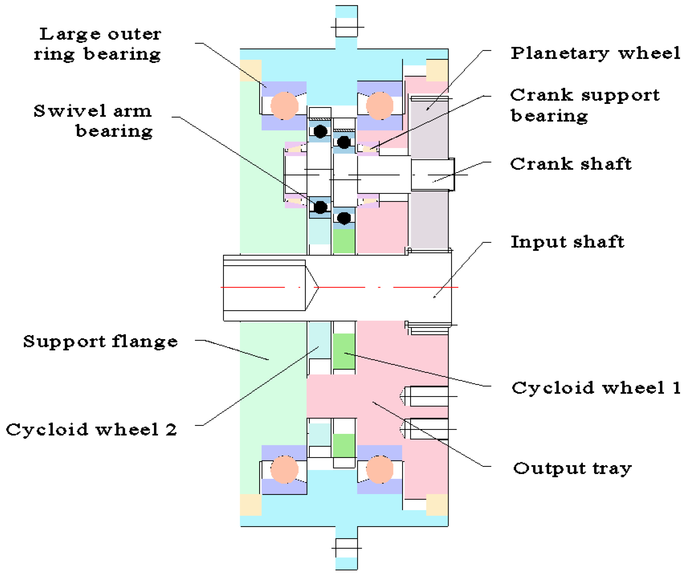
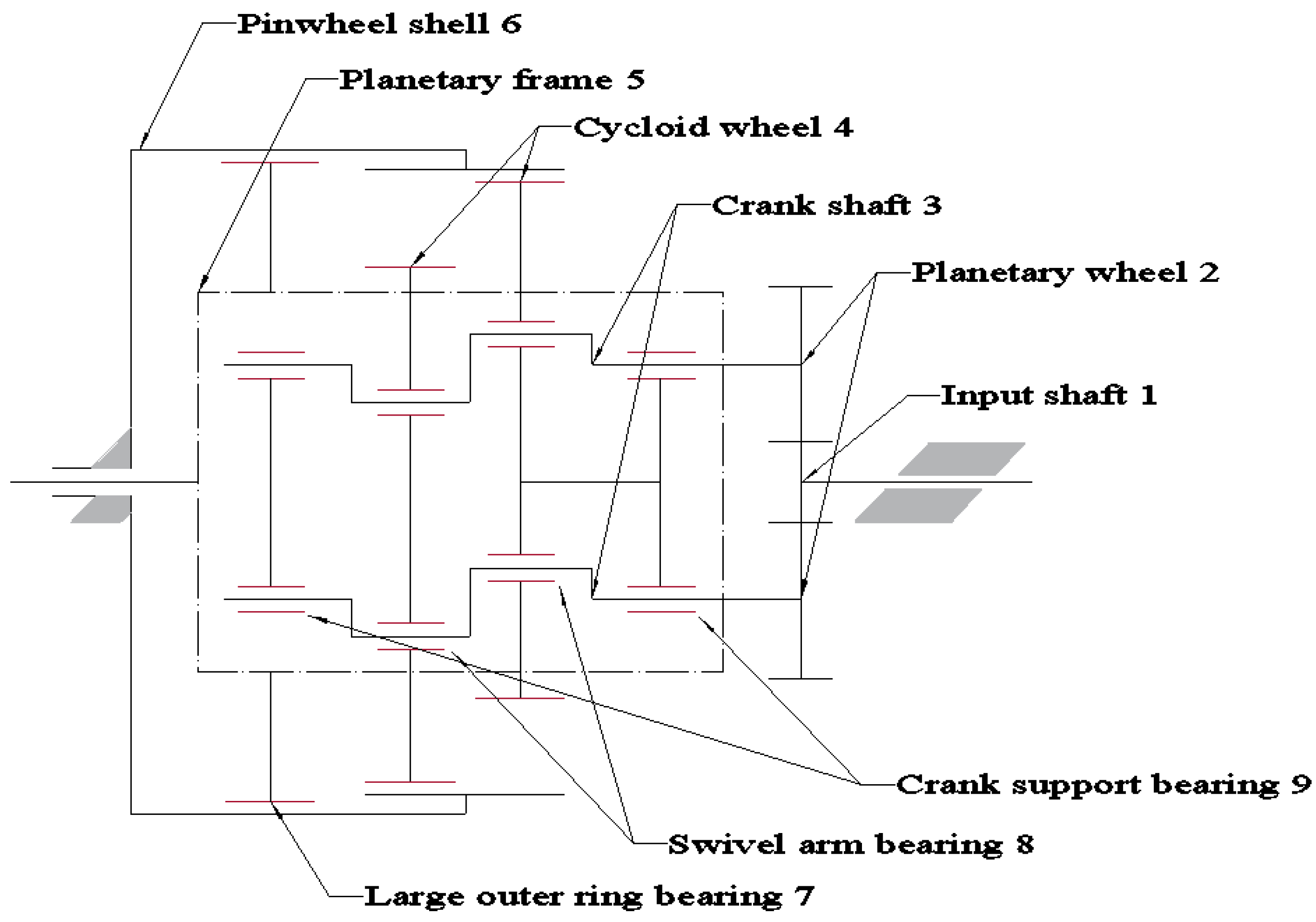
An RV reducer is generally composed of two stages: the front stage is a planetary wheel drive, and the rear stage is a cycloid pinwheel drive. The primary planetary wheel drive mechanism mainly includes a sun wheel and three planetary wheels, and the secondary cycloid pinwheel drive mechanism’s main components are a cycloid wheel, crankshaft, pinwheel, planetary frame, and pinwheel shell (a structural sketch and a transmission structure sketch of an RV reducer are shown in Figure 1 and Figure 2, respectively). Therefore, force analysis between the components in the transmission process is complicated [19].
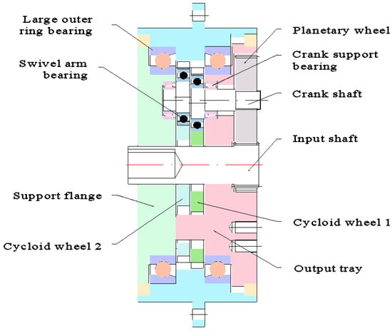
Figure 1.
Diagram of a certain type of RV reducer.
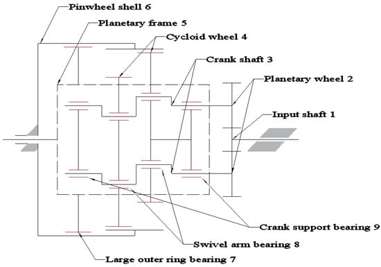
Figure 2.
Transmission diagram of RV deceleration.
To facilitate the calculation, we established a force analysis coordinate system, as shown in Figure 3.
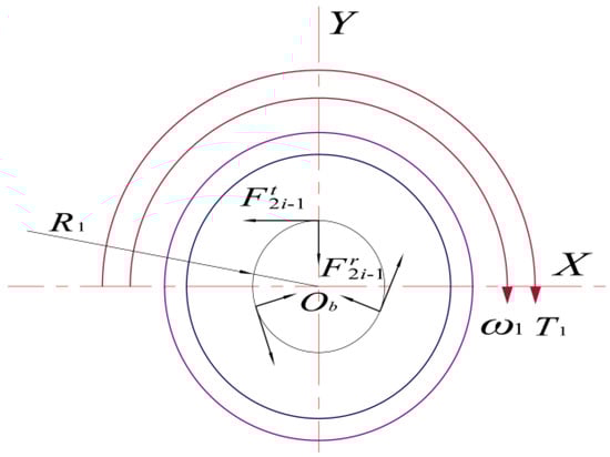
Figure 3.
Coordinate system of the total action force analysis.
The figure shows a coordinate system with the Y-axis passing through the center of a planetary wheel in the positive upward direction; the X-axis is in the positive rightward direction, and the Z-axis is in the positive outward direction perpendicular to the paper’s surface, using the center of the RV reducer Ob as the coordinate origin.
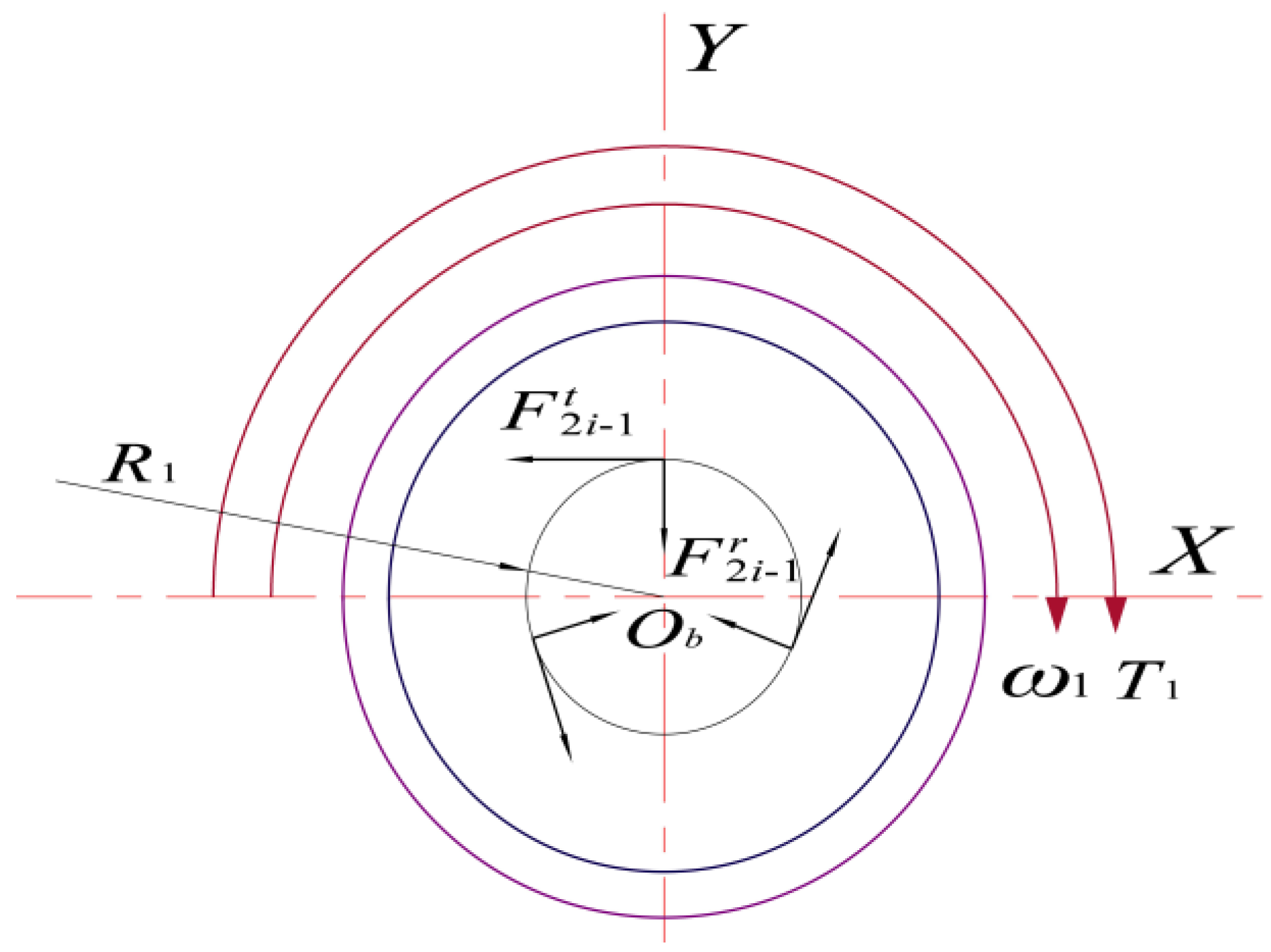
2.1. Analysis of Input Shaft Force
The center wheel at one end of the input shaft transmits the load by meshing with n (n > 1) planetary wheels, and the planetary wheels 2i (i = 1, 2, …, n) share the load of the input shaft equally between them, with an angle of 120° between them. The specific force transfer structure (let there be a total of 3 planetary wheels) is shown in Figure 4.
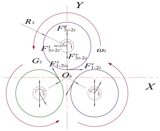
Figure 4.
Force transmission diagram of the planetary wheel and the input axis.
Combining this with Figure 3, the meshing points of the sun wheel 1 and the planetary wheel 2i rotate with the planetary wheel 2i in a certain time t(s) while the planetary frame 5 is rotating via self-propagation. Then, the force analysis of the input shaft center Ob is carried out, and the vector expression for the force of the planetary wheel on input axis 1 can be written as follows:
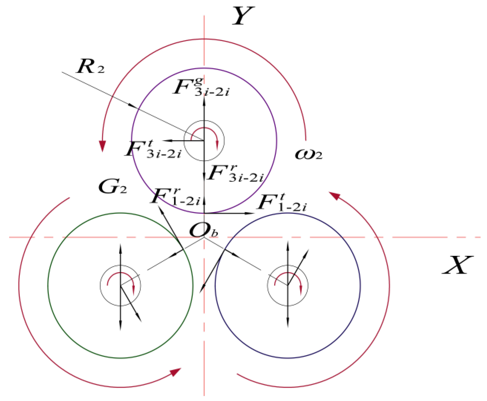
2.2. Analysis of Planetary Wheel Forces
As shown in Figure 4, planetary wheel 2i is not only subjected to force from input shaft 1 but also receives force from crankshaft 3i. For the force analysis of the center of planetary wheel 2i, the forces and moments are in the same plane.
From the structure of the reducer and Figure 4, it can be seen that the force on planetary wheel 2i from crankshaft 3i rotates with the crankshaft’s rotation, that is, with the rotation of planetary frame 5, and then the vector expression of the force on planetary wheel 2i from crankshaft 3i can be given as follows:
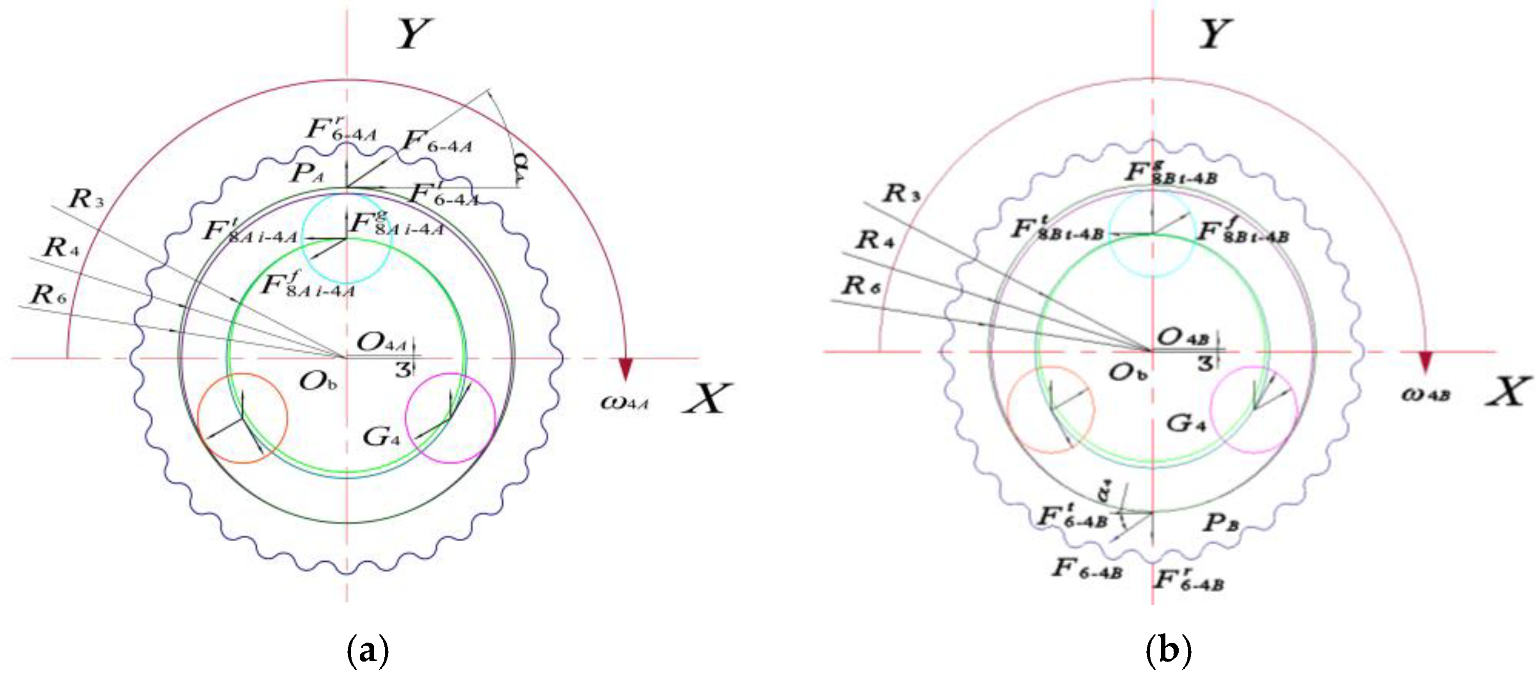
2.3. Analysis of Cycloid Wheel Force
Cycloid wheel 4 is in contact with swivel arm bearing 8 and the pinwheel. The specific force transfer diagrams between cycloid wheel 4, swivel arm bearing 8, and the pinwheel were shown in the following figures.
The force on the pinwheel on cycloid 4A points to node PA, and the force on cycloid 4B points to node PB (the combined force of multiple pinwheels is simplified). Since the positions of the two cycloid wheels are conjugately distributed, the forces are equal in magnitude and opposite in direction, as shown in Figure 5a,b.
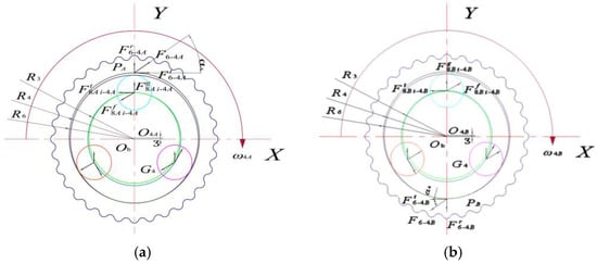
Figure 5.
(a) Schematic diagram of cycloid wheel 4A. (b) Schematic diagram of cycloid wheel 4B.
The force analysis of cycloid wheels 4A and 4B was performed using the following:
In Equation (3), α4 is the shift wheel pressure angle, n2 is the number of planetary wheels, and G4 is the gravity in part 4.
Therefore, the force expression of rotating arm bearing 8Ai on cycloid wheel 4A can be written as follows [6]:
The force expression of rotating arm bearing 8Bi on cycloid wheel 4B can be given as follows:
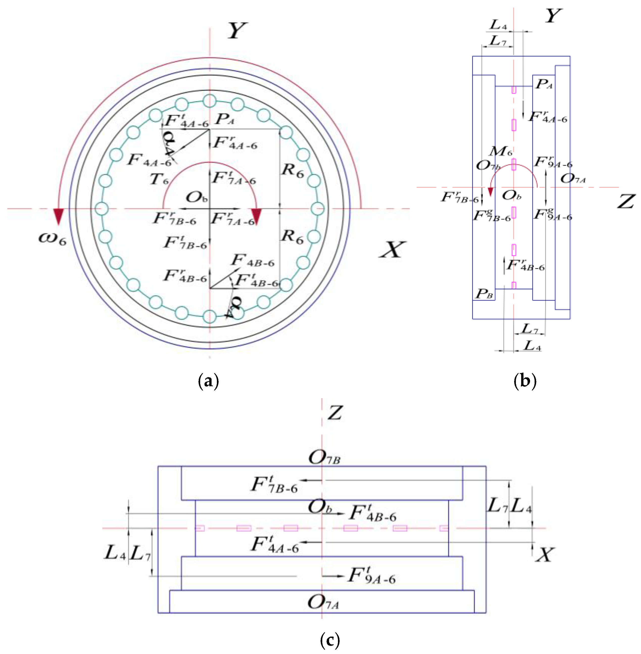
2.4. Analysis of the Needle Tooth Shell Force
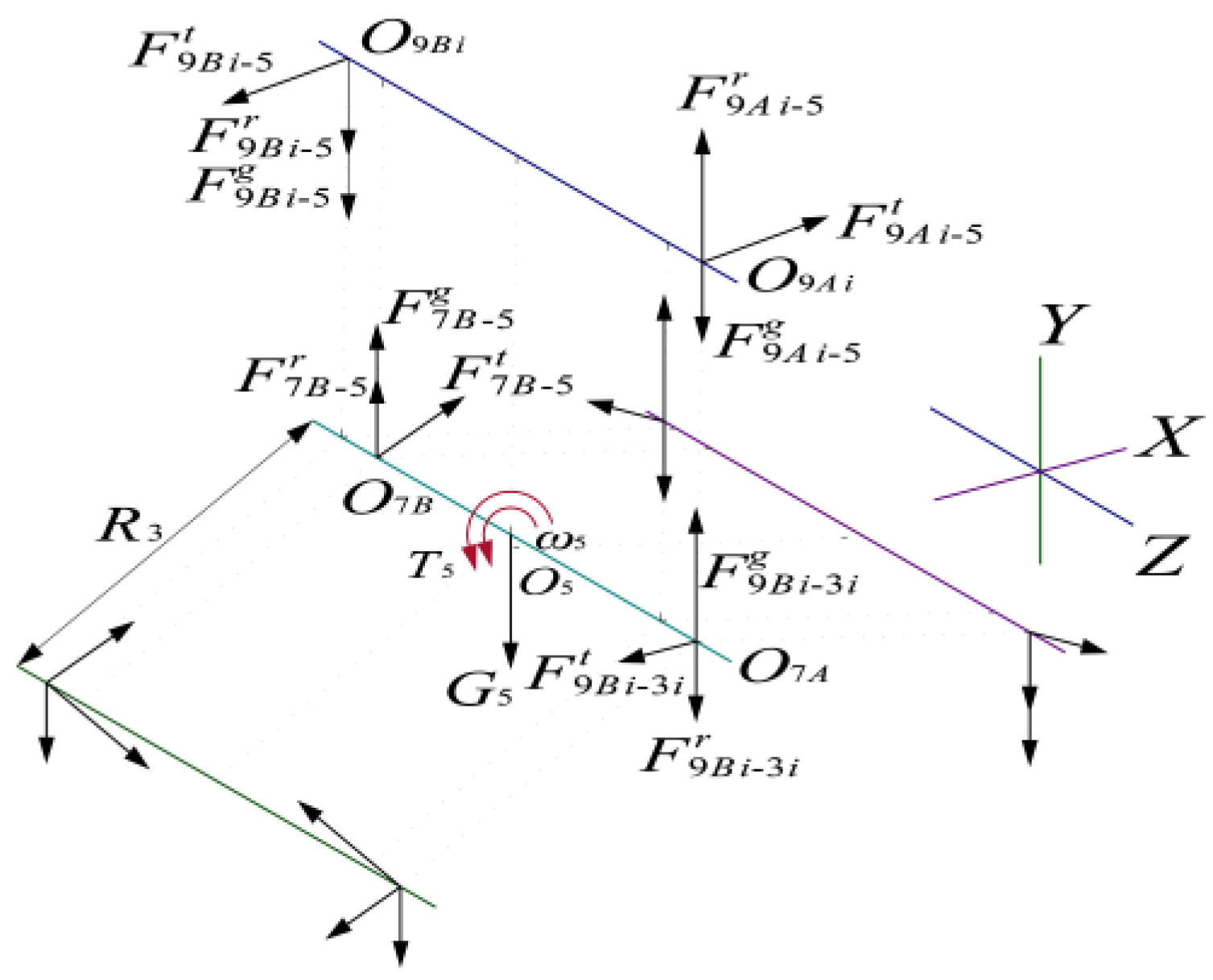
The pinwheel is composed of a needle tooth case and needle teeth. Its main force comes from cycloid wheel 4 and the outer ring bearing (reducer main bearing). The specific force diagram is shown Figure 6.
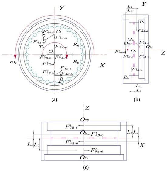
Figure 6.
Schematic diagram of the force on the needle tooth shell.
According to the schematic diagram of the X-Ob-Y plane (a), the force analysis is performed at the center Ob of the pinwheel; according to the schematic diagram of the Y-Ob-Z plane (b) and the X-Ob-Z plane (c), the force analysis is performed at the centers O9A and O9B of the main bearings 9A and 9B, respectively, to obtain the following:
The force of the main bearings 7A and 7B on the needle tooth housing can be written as follows:
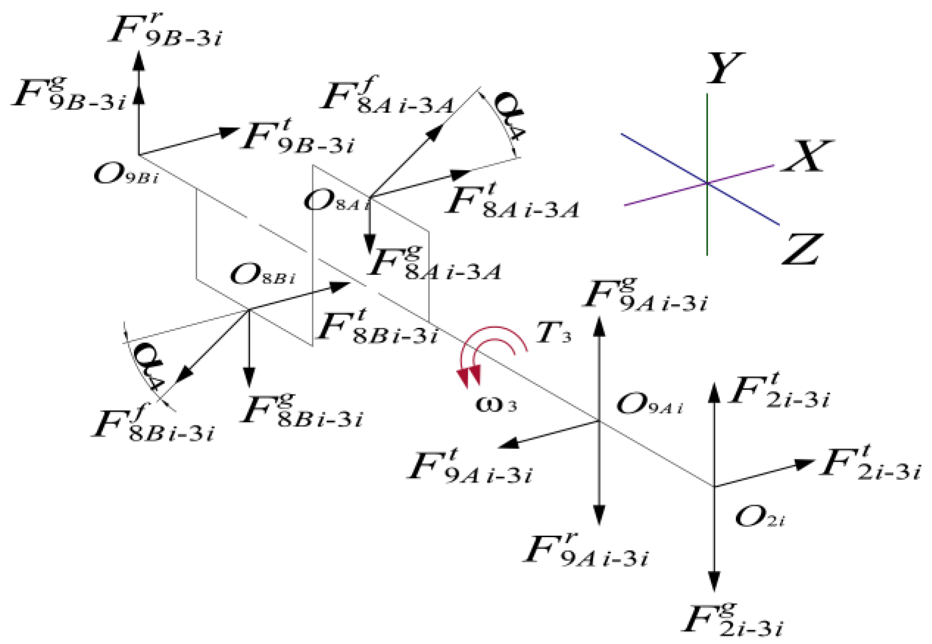
2.5. Analysis of the Crankshaft Force
Crankshaft 3i is mainly subjected to forces from three main components, namely, planetary wheel 2i, support bearing 9i, and swivel arm bearing 8i, as shown in the following diagram.
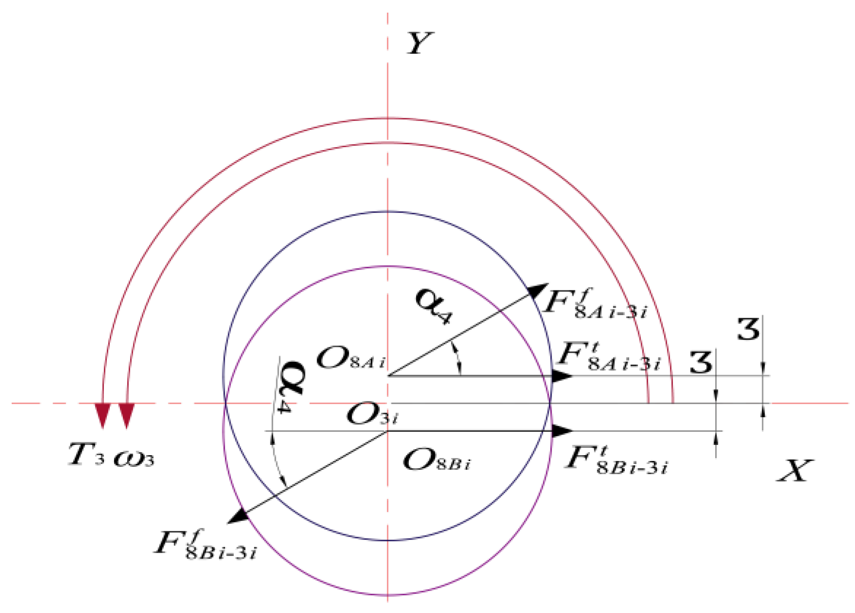
By projecting Figure 7 onto the X-Y plane, the crankshaft is projected onto the X-O3i-Y plane by the forces of the swivel arm bearings 8Ai and 8Bi, as shown in Figure 8.
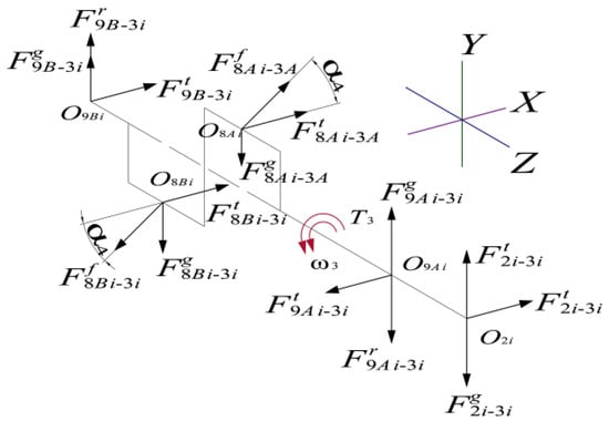
Figure 7.
Diagram of the crankshaft force.
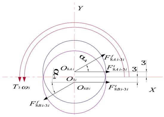
Figure 8.
Schematic diagram of the force bearing in the X-Y direction of the crank axis.
In the equation, “a” represents the eccentricity distance.
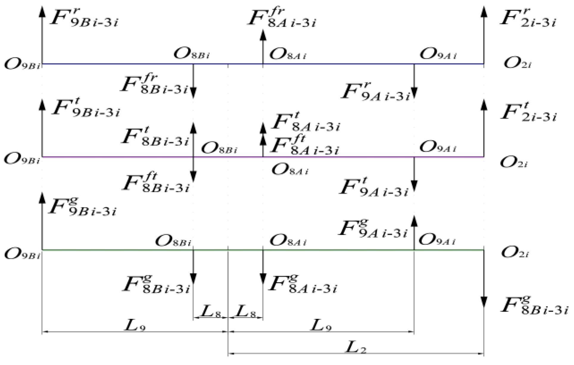
Figure 8 is then projected onto the Y-Z plane to obtain a force schematic of the crankshaft in the Y-Ob-Z plane (divided into three parts for ease of observation), as shown in Figure 9.
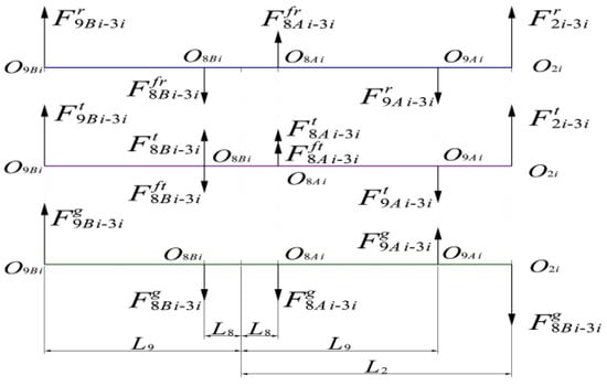
Figure 9.
Schematic diagram of the force bearing in the Y-Z direction of the crank axis.
Force analysis at points O8Ai, O8Bi:
Radial bending moment balance:
Tangential moment balance [10,14]:
Vertical moment balance:
In Equations (13) and (14), LX is the Z-direction distance from the center of Part X to the coordinate origin.
2.6. Analysis of Planetary Frame Forces
The input and output flanges together form planetary frame 5, which is mainly subjected to forces from the crank support bearings 8Ai and 8Bi and the main bearings 9A and 9B. A diagram of the forces is shown in Figure 10.
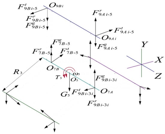
Figure 10.
Schematic diagram of the force of the planetary frame.
Balance of vertical moment at point O9A:
Balance of vertical moment at point O9B:
2.7. Theoretical Visualization
Some parameters of the speed reducer and three typical working conditions are shown in Table 1 and Table 2.

Table 1.
Parameters of an RV reducer.
Table 2.
Load spectrum of an RV reducer.
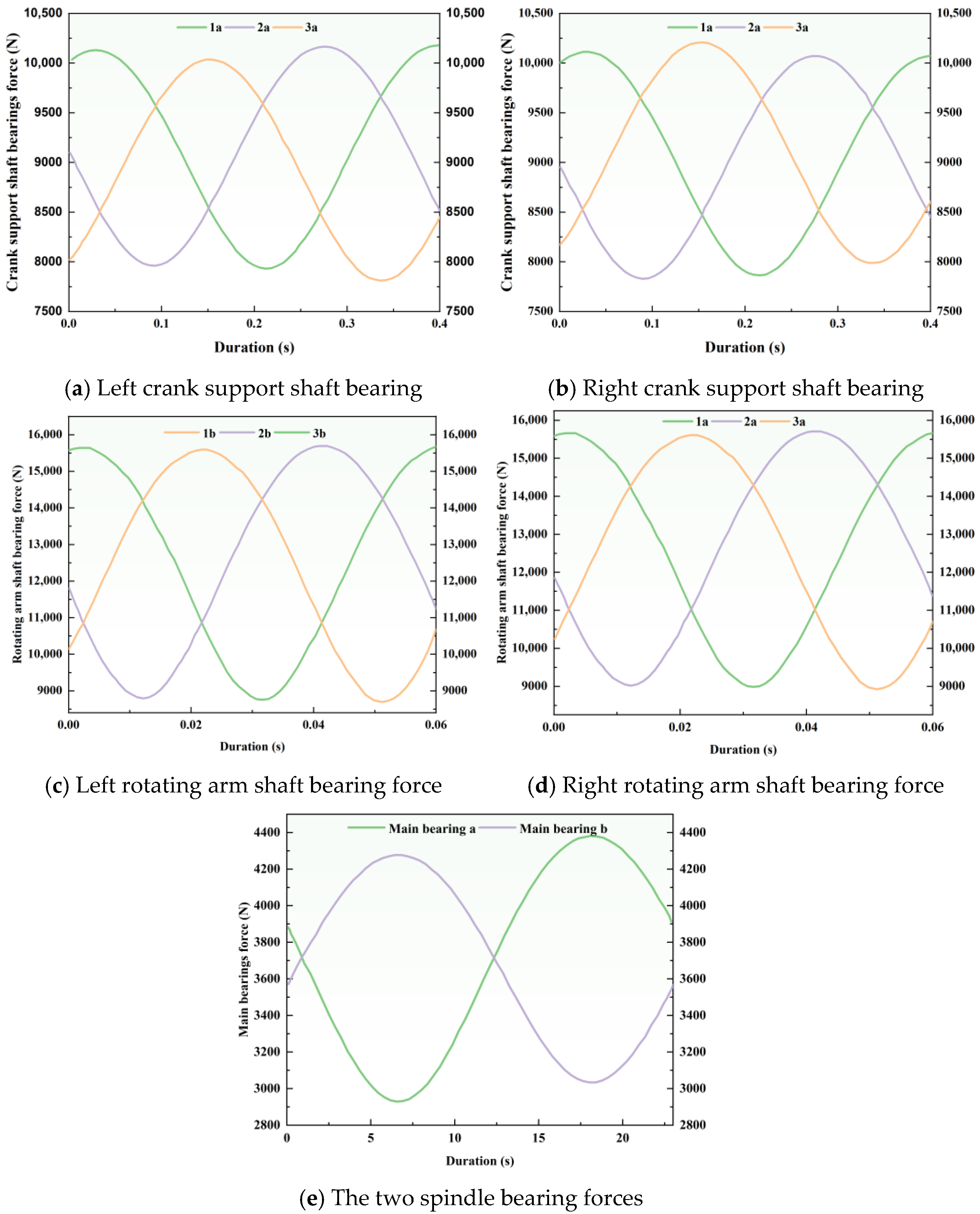
By visualizing the model and introducing the rated working conditions (output speed: 15 rpm, torque: 3136 N·mm) and reducer structure parameters, the theoretical load spectra of three types of bearings were obtained.
In Figure 11a–e, it can be seen that the load spectra of the three bearings of the RV reducer are approximately sinusoidal, and the force on the swivel arm shaft is the largest among the three bearings, followed by that of the crank support bearing, with that of the main bearing being the smallest.
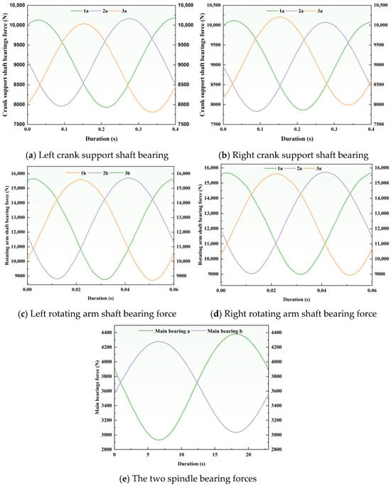
Figure 11.
Bearing load in A360 RV reducer type III.
For the crank support bearing, after a week in a relative rotation state, as shown in Figure 11a,b, its force sinusoidal curve changes, and the bearing force on the same side of the shaft has a phase difference of 120. Both sides of the bearing force are basically the same; the average force is about 9000 N, the change amplitude is about 2200 N, and the maximum value is about 10,200 N.
The force state of the swivel arm bearing when it is rotated for one week is shown in Figure 11c,d. The force state is the same as that of the crank support bearing, the average force is about 12,300 N, the variation is about 6600 N, and the maximum value is about 15,700 N.
Two main bearings in a state of relative rotation of the force for a week are shown in Figure 11e; the sinusoidal curve of the bearing force changes, the two sides of the spindle bearing force change in the opposite way, and the average force is about 3700 N, but in consideration of the influence of gravity, the two spindle bearing force change amplitudes are different. Near the planetary wheel side of the main bearing, the change amplitude is about 1500 N, and the maximum value is about 4400 N. Near the side of the support flange of the main bearing, the change amplitude is about 1300 N, and the maximum value is about 4300 N.
3. Simulation Experiments with Three Types of Shaft Bearing Forces
In combination with a finite element analysis software, the calculations in the theoretical analysis are verified, and the changes in the shaft bearing force under different working conditions are analyzed.
3.1. Load Spectra of Three Types of Bearings Under Three Working Conditions
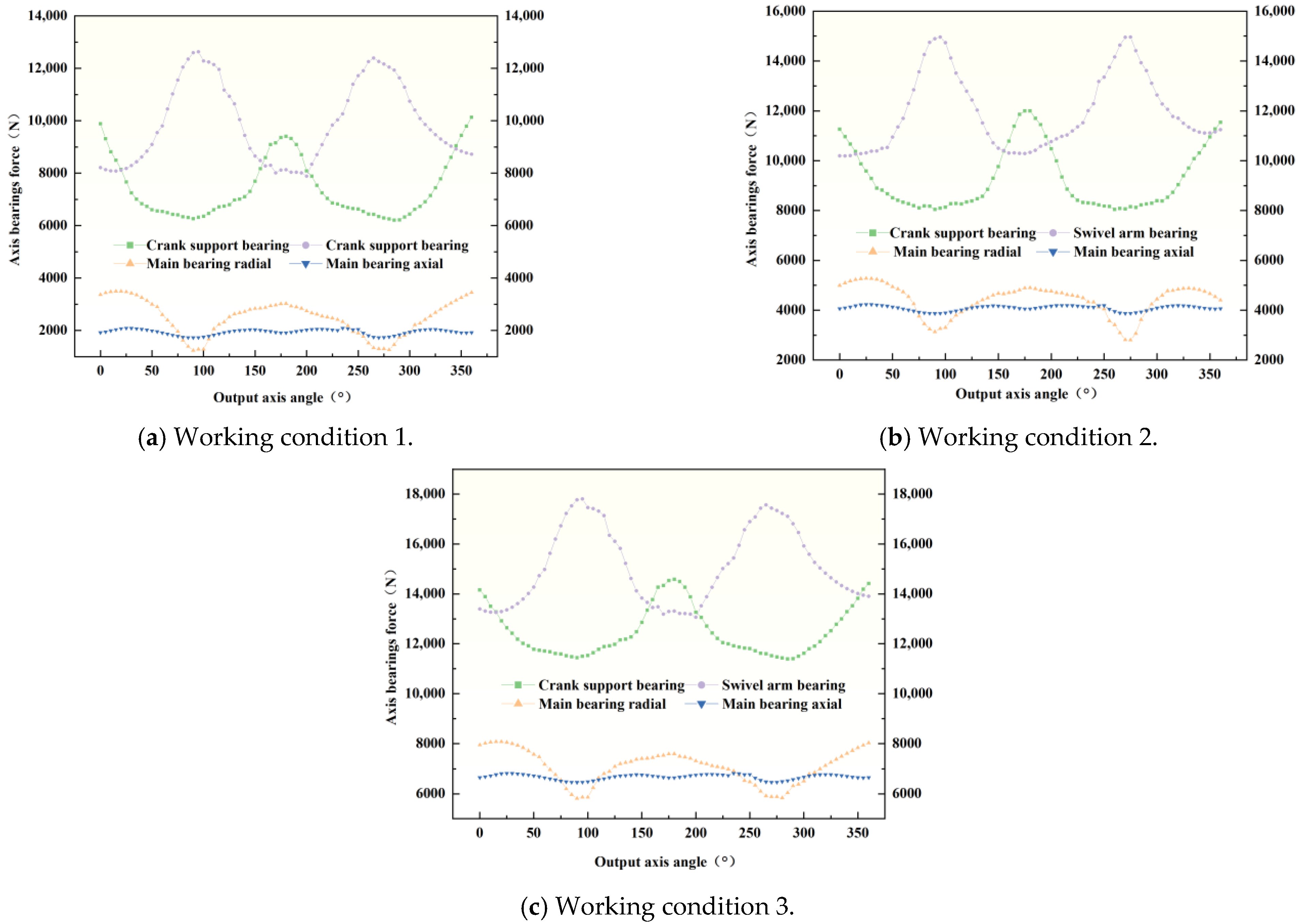
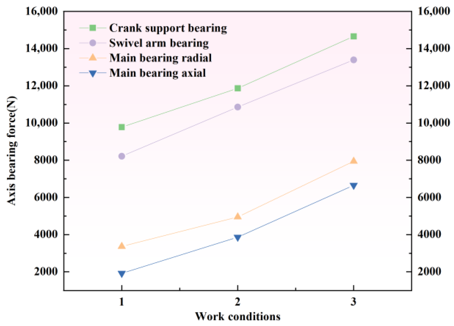
The reducer is loaded according to the working conditions given in Table 2; the load spectra of the three bearings under the three working conditions are obtained, and the change trend under the three working conditions when the corresponding output shaft rotation angle is 0 is summarized, as shown in Figure 12 and Figure 13, respectively.
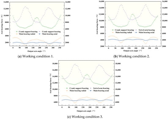
Figure 12.
Bearing load spectrum of A360 RV reducer type III under the three working conditions.
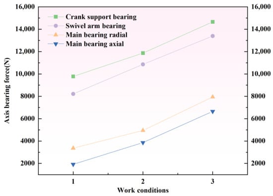
Figure 13.
Changes in the shaft bearing force under the three working conditions (when the output shaft rotation angle is 0 degrees).
① The three types of bearing loads are cyclic, which is consistent with the theoretical calculations, thus indicating the validity of the simulation model.
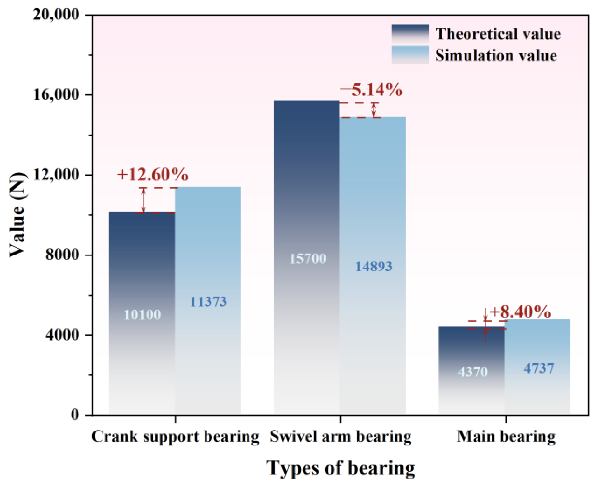
② The rotating arm shaft is subjected to the largest force (5.14% smaller than the theoretical calculated value), the crank support bearing is subjected to the second largest (12.60% larger than the theoretically calculated value), and the main bearing is subjected to the smallest (8.40% larger than the theoretically calculated value); specific pair ratios are shown in Figure 14.
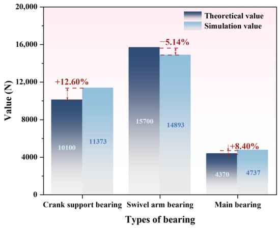
Figure 14.
Comparison of theoretical and simulated values at the rated working conditions.
③ The main bearing’s axial load does not vary much.
④ The radial load cycle of the main bearing varies with a large amplitude of load change.
⑤ With the increase in torque, the forces on these bearings all increase.
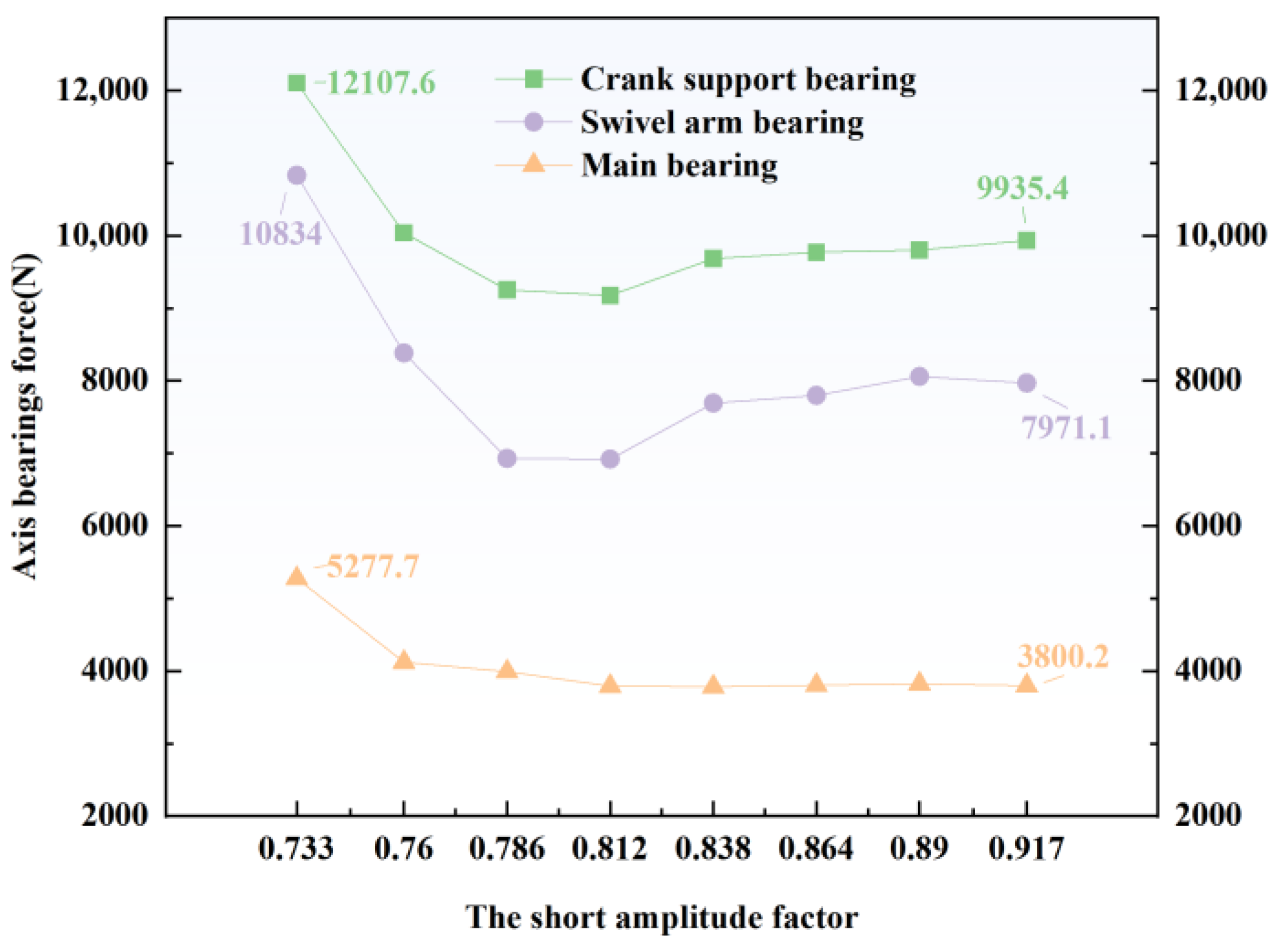
3.2. Influence of a Short Amplitude Factor on the Three Kinds of Shaft Bearing Forces Under the Rated Working Conditions
The short amplitude coefficient is an important parameter of the planetary transmission of a cycloid pinwheel. When the radius of the pinwheel distribution circle and the number of pinwheel teeth are certain, the main parameter that affects the profile of the cycloid teeth and the bearing capacity is the short amplitude coefficient, which can be chosen in the design process in order to obtain the best transmission performance, and whether its value is appropriate also directly affects the value of other design parameters, which, in turn, affects the performance of the reducer [20,21]. Therefore, it is of great engineering significance to investigate the influence of the short amplitude factor on the bearing load carrying capacity.
In combination with a method of determining the short amplitude factor, this study was carried out by varying the number of pinwheels and the radius of the knuckle circle of the cycloid wheel. The resulting load variations for the three types of bearings with different short amplitude factors are shown in Figure 15.
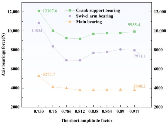
Figure 15.
Effect of the short amplitude coefficient on shaft bearing force (when the output shaft angle is 0 degrees).
In Figure 15, it can be seen that when the short amplitude coefficient δ is larger, the crank support bearing and the swivel arm bearing first decrease and then increase, and the main shaft bearing capacity first decreases and then tends to be constant. When the short amplitude coefficient δ is 0.786, the bearing capacity of the three shafts is the smallest, which means that the bearing has better bearing capacity than the RV reducer at this time.
When the short amplitude coefficient is increased from 0.733 to 0.786, the number of instantaneous contact points between the cycloid wheel and the needle teeth transitions from double-tooth contact to single-tooth contact. This contact stress concentration leads to an increase in the bearing radial force. However, at δ = 0.786, a unique contact distribution of “three peaks” is formed, which creates a dynamic balance between the load at the crank support bearing and the swivel arm bearing. At this point, the system’s stiffness matrix exhibits a singularity, and the bearing capacity reaches its minimum value. The rate of change of the axial bearing capacity of the main bearing approaches zero when the short amplitude coefficient exceeds 0.812, which aligns with the nonlinear relationship between the crankshaft phase lag angle θ and the findings in [22].
When δ ≥ 0.812, θ enters the saturation region, causing the axial force to stabilize.
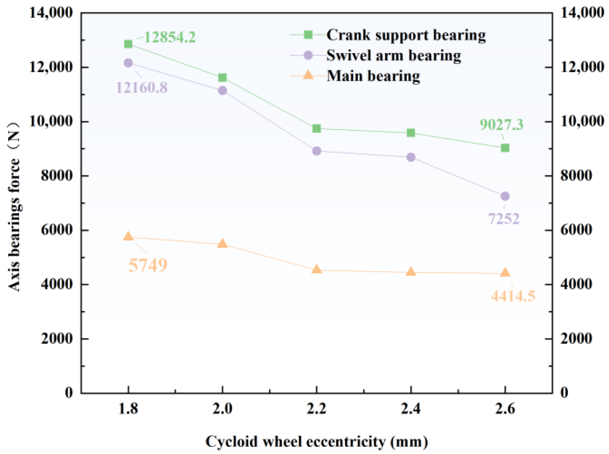
3.3. Influence of Cycloid Wheel Eccentricity on the Bearing Force of Three Shafts Under the Rated Working Conditions
The cycloid wheel eccentricity has a critical influence on the maximum contact stiffness between the cycloid and the pinwheel, which can be directly related to the load carrying capacity of the mechanism [22,23]. Therefore, in order to investigate the force state of the bearing, it is essential to study the influence of the cycloid wheel eccentricity on it. According to the structure of the reducer, the analysis was carried out using cycloid wheel eccentricities between 1.8 and 2.6 mm, and finally, the load spectrum and load variation of the three types of bearings under different cycloid wheel eccentricities are shown in Figure 16.
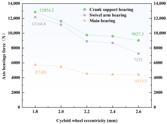
Figure 16.
Effect of cycloid wheel eccentricity on the shaft bearing force (when the output shaft angle is 0 degrees).
In Figure 16, it can be seen that as the cycloid wheel eccentricity increases from 1.8 mm to 2.6 mm, increasing by 44.40%, the forces on the crank support bearing, the swivel arm bearing, and the main shaft bearing decrease by 30.70%, 40.80%, and 24.10%, respectively, and they approximate a linear relationship. It can be seen that the increase in eccentric distance is beneficial to the forces on these bearings. An increase in eccentric distance significantly alters the engagement phase between the cycloid wheel and the needle teeth. A larger eccentric distance causes the cycloid wheel to generate more simultaneous contact points with the needle teeth during its motion, thereby distributing the load across more needle teeth. This multi-tooth contact effect reduces the instantaneous peak load on the individual bearings. However, the precise and compact structure of the reducer makes it so that the eccentric distance cannot be too large, so the law can only be used for reference when designing a reducer.
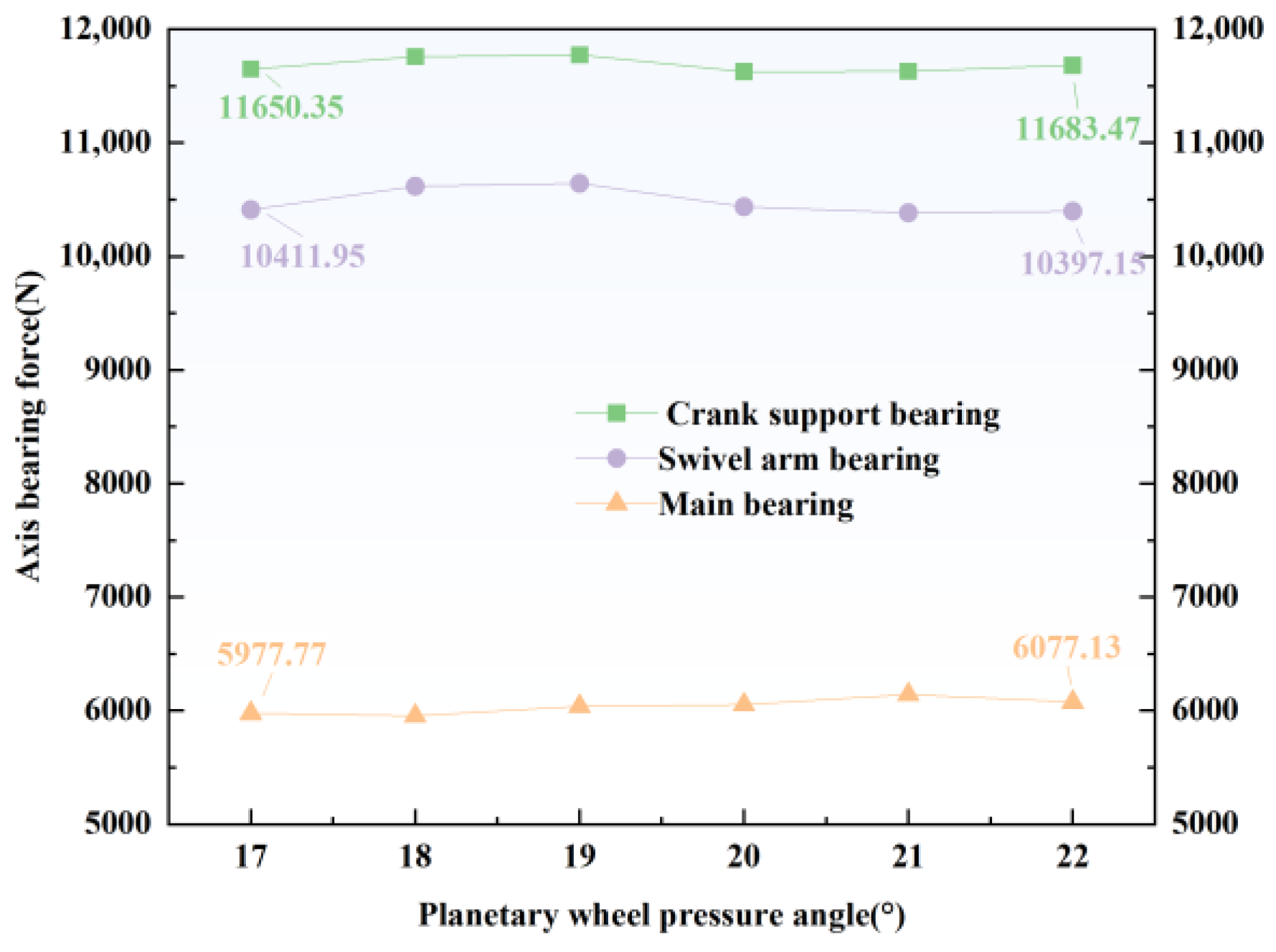
3.4. Influence of the Planetary Wheel Pressure Angle on the Three Shaft Forces Under the Rated Operating Conditions
The pressure angle is an indicator for evaluating mechanism dynamics [24], and its influence on the gearbox transmission is not small, so it is also essential to study the influence of the planetary wheel pressure angle on the bearing load spectrum. The variations in the three bearing loads for different pressure angles are shown in Figure 17.
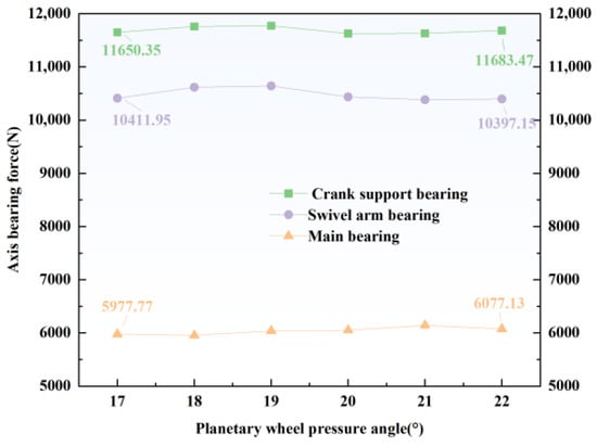
Figure 17.
Influence of the planetary wheel pressure angle on the shaft bearing force (when the output shaft angle is 0 degrees).
In Figure 17, it can be seen that as the planetary wheel pressure angle increases from 17 mm to 21 mm, the radial forces of the crank support bearing, swivel arm bearing, and main bearing remain essentially unchanged. It can be observed that the impact of the planetary wheel pressure angle on the bearing forces is minimal. The RV reducer employs a two-stage enclosed transmission structure, with the planetary wheel system serving as the first-stage reduction mechanism. Its power is transmitted through the crankshaft to the second-stage cycloid pinwheel mechanism. Most of the radial force generated by the planetary wheel meshing is transmitted directly to the reducer housing through the planetary carrier, with only a small portion of residual fluctuations being transmitted to the crankshaft system. This layered structural design creates effective mechanical isolation, causing changes in the planetary wheel pressure angle to primarily affect the contact stress distribution in the planetary wheel–sun wheel meshing area, with limited impact on the radial force transmission path of the internal crankshaft support bearings. Therefore, the impact on the internal bearings of the reducer is much smaller.
3.5. Influence of the Needle Tooth Coefficient on the Three Kinds of Shaft Bearing Force Under the Rated Working Condition
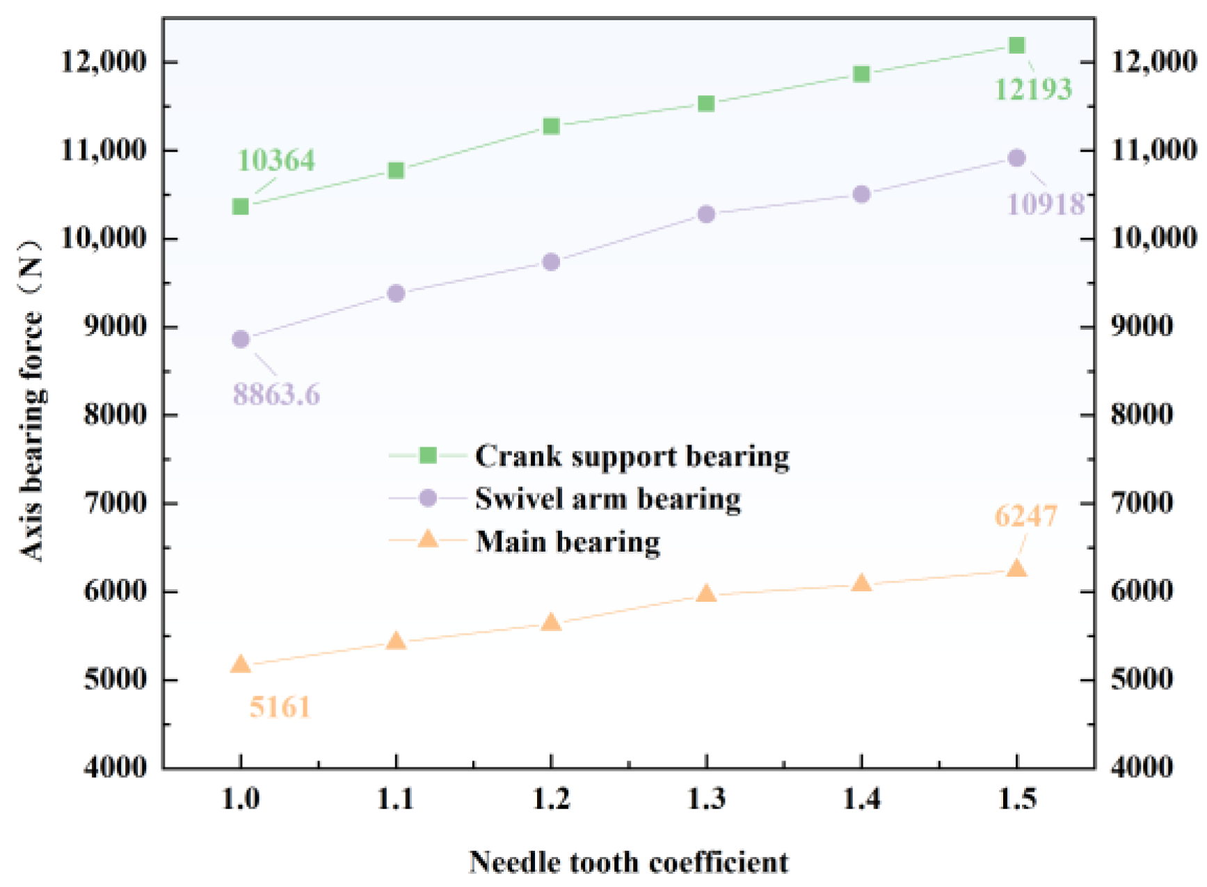
The needle tooth coefficient E is the ratio of the distance between the centers of two adjacent needle teeth to the diameter of the needle teeth in the end plane of the pinwheel [25]. The force variations of the three types of bearings with different needle tooth coefficients are shown in Figure 18.
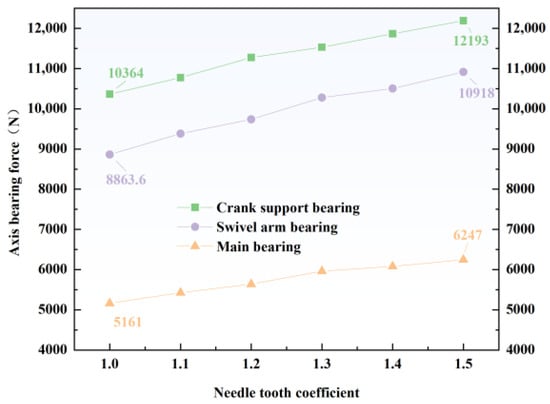
Figure 18.
Effect of the needle tooth coefficient on the shaft bearing force (when the output shaft rotation angle is 0 degrees).
It can be seen in the figure that as the needle tooth coefficient increases from 1.0 to 1.5 (by 50%), the forces on all three types of bearings become larger in a linear fashion, with the forces on the crank support bearing, the swivel arm bearing, and the main bearing increasing by 17.90%, 23.70%, and 20.40%, respectively, thus demonstrating a strong correlation. As the needle tooth coefficient increases, meaning that the needle tooth radius decreases, the equivalent curvature radius of the cycloid wheel’s tooth profile and the needle tooth’s curvature radius will decrease. If the meshing load remains unchanged, the maximum stress in the contact area will significantly rise. To avoid exceeding the contact stress limit, it is necessary to increase the contact area to reduce the stress. However, the geometric constraints of the RV reducer cause the contact force to inevitably increase, thereby transferring it to each bearing.
3.6. Influence of the Planetary Wheel Ratio on the Three Shaft Forces Under the Rated Operating Conditions
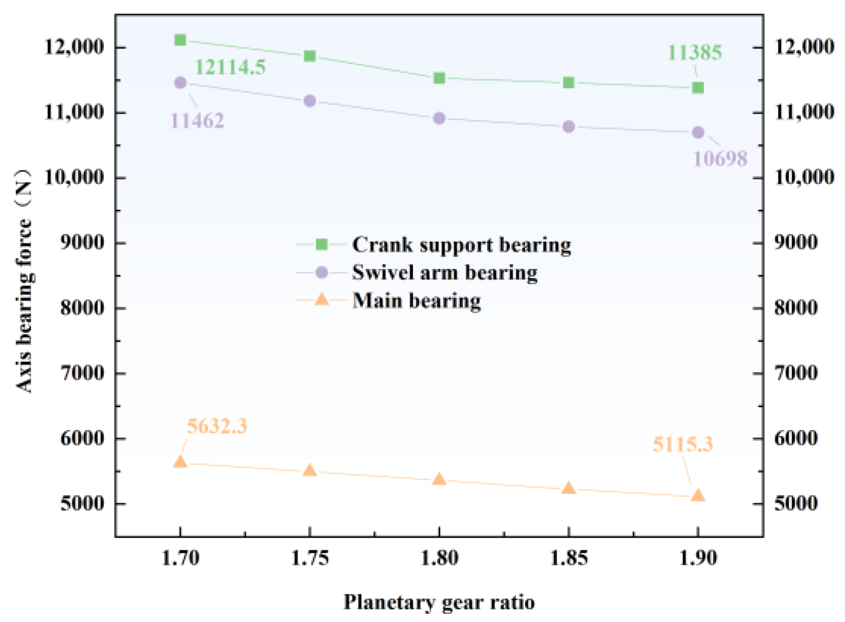
As the first-level transmission mechanism of the gearbox, the transmission performance must have a significant impact on its overall force. The force variations of the three types of bearings according to the planetary wheel ratio are shown in Figure 19.
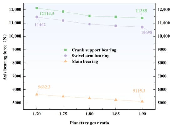
Figure 19.
Effect of the transmission ratio on the shaft bearing force (when the rotation angle of the output shaft is 0 degrees).
The figure shows that as the planetary wheel ratio increases from 1.7 to 1.9 (by 11.76%), the forces on all three types of bearings decrease linearly, with the forces on the crank support bearing, the swivel arm bearing, and the main bearing decreasing by 6.02%, 6.70%, and 9.20%, respectively. The increase in the transmission ratio leads to a reduction in the gear meshing force, which, in turn, reduces the torque applied to the crankshaft and, ultimately, has an effect on the bearing forces.
3.7. Influence of the Width of the Cycloid on the Bearing Force of the Three Shafts Under the Rated Working Conditions
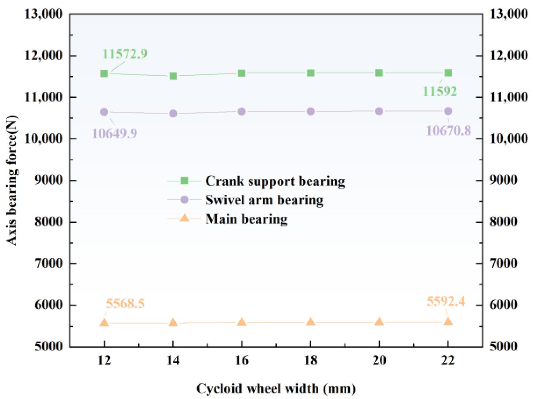
The width of the cycloid is related to its contact performance when it engages with the needle teeth during the cycloid drive [26]. The force variations of the three types of bearings at different cycloid widths are shown in Figure 20.
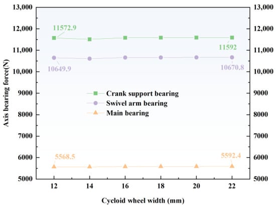
Figure 20.
Effect of the cycloid wheel width on the shaft bearing force (when the rotation angle of the output shaft is 0 degrees).
As can be seen in the diagram, as the cycloid wheel width increases from 12 mm to 22 mm, there is no significant change in the force experienced by the three types of bearings. The contact force between the cycloid wheel and the needle teeth is primarily determined by the torque transmitted by the system, rather than the contact area. According to Hertzian contact theory, the contact radius increases with the cycloid wheel width, and the increase in contact area reduces the contact stress. However, the contact force is still dominated by the external load (torque). Therefore, the width of the cycloid wheel has a minimal impact on the bearing forces and a small effect on the contact force.
4. Structural Optimization and Design of an RV Reducer Based on Kriging-NSGA-II
The findings in Section 1 and Section 2 show that the structural parameters of a reducer have a certain influence on the force on the bearings. Therefore, by performing a reasonable structural optimization of a reducer, the load on the three types of bearings in operation can be reduced, thus extending their service life. In this section, based on the above mechanical model, the working load of the three types of bearings in an RV reducer during operation is taken as the objective function, and the multi-objective optimization process is simplified by establishing a Kriging agent model of the three types of bearing loads. The multi-objective optimization model of the reducer bearings is solved by using the NSGA-II algorithm, and the reducer bearing loads before and after optimization are compared and analyzed to verify the optimization results.
4.1. Optimized Design Model for a Reducer
4.1.1. Objective Function
For the bearing of a reducer, low load is an important indicator that the reducer is not easily damaged during long-term operation. Therefore, in this study, Table 1 and Table 2 are used as references for the structure and working parameters of the reducer, and the crank support shaft bearing force, swivel arm shaft bearing force, and main shaft bearing force are selected for the objective function of the optimized design as follows:
4.1.2. Design Variables and Constraints
The load during the operation of the three types of bearings is influenced by many factors, such as the internal structural parameters of the reducer. The optimized design in this study mainly focuses on the internal structural parameters of the reducer, without considering the influence of changes in operating conditions and other factors on the objective function.
From the above analysis, it can be seen that the crank support shaft bearing force, the swivel arm shaft bearing force, and the main shaft bearing force can be expressed using several main structural parameters of the reducer:
(1) Constraints on the needle tooth coefficient E:
The values of the needle tooth coefficient E were chosen according to the literature [27], and the specific range of values is shown in Table 3.
Table 3.
The range of values of the needle tooth coefficient E.
(2) Constraints on the width B of the cycloid
The thickness of the cycloid wheel is generally taken within the range of 0.1 Ra~0.2 Ra. The following are the constraints on the thickness of the cycloid wheel:
(3) Short amplitude factor K constraint
A reasonable range of values for the short amplitude factor is shown in Table 4.
Table 4.
Range of values of the short amplitude factor.
As shown in Table 4, if [a1,a2] is used to represent the range of values of the short amplitude coefficients, the constraint equation can be expressed as follows:
(4) Constraints on the cycloid wheel eccentricity e
Because the cycloid wheel eccentricity is , it can be treated as a process variable when performing optimization.
(5) Constraints on the planetary wheel pressure angle α
The conditions for gears not to produce root cut are
Then, the range of the pressure angle is
(6) Constraints on the planetary wheel ratio
Due to the size constraint on the reducer, the transmission ratio of the planetary wheel cannot be too large, so the range of the transmission ratio is 1.65–1.85.
The original design values and the ranges of values of the variables to be optimized for the internal structural parameters of the reducer are shown in Table 5.
Table 5.
The original design values and value ranges of the variables to be optimized.
4.2. Optimization Methods and Optimization Models
4.2.1. Principle of the Kriging Agent Model
The Kriging proxy model is a semi-parametric interpolation technique that is used to perform linear regression analysis on sample points. It has the characteristics of not being restricted by the form of the state function and being good at solving strong nonlinear problems with a short time consumption [28].
Since the calculation of the three types of shaft forces in the reducer involves finding the equilibrium equations between each component, the intermediate process is complex, strongly nonlinear, and time-consuming. Therefore, Kriging proxy models for each of the three types of shaft forces are developed separately to reduce the time required for multi-objective optimization [29]. The Kriging model assumes that the response value of the system and the design variable can be represented by the following equation:
Z(x) is a stochastic process function whose statistical characteristics can be expressed as
Here, is the correlation function of the sample points, and the Gaussian correlation equation is usually chosen to express the following:
The prediction model at sample point x can be expressed as follows:
Sample data play a crucial role in the accuracy of Kriging models, and the construction of Kriging models requires that the sample data used feed back as much information as possible about the local space. In general, the number of sample points required for Latin hypercube sampling is 5–10 times the number of variables to be optimized [30]. The Kriging model is built using the dace toolbox, and the complex correlation coefficient and root mean square error are commonly used as measures to evaluate the fitting accuracy of the Kriging proxy models. Their expressions are as follows:
4.2.2. NSGA-II Multi-Objective Optimization Algorithm
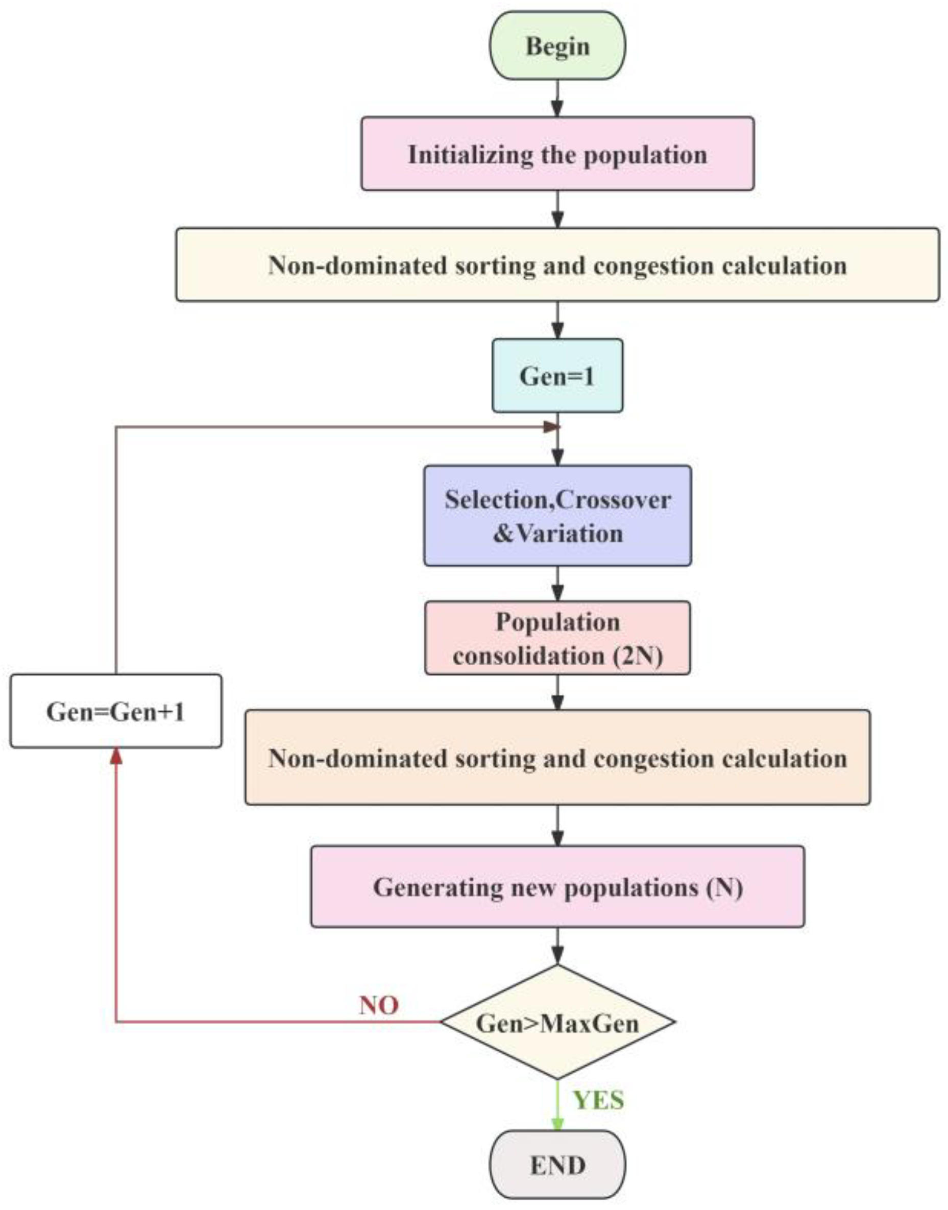
NSGA-II is an algorithm proposed by Deb [31] for solving multi-objective optimization problems. The algorithm adds non-dominated sorting and crowding calculation to the traditional genetic algorithm, and it performs non-dominated sorting and genetic operations on the initialized population to generate the next-generation population, then merges the initial child population with the parent population, repeats the above operations until the end of the cycle, and obtains the Pareto frontier set composed of non-dominated solutions [32,33]; a specific flowchart thereof is shown in Figure 21.
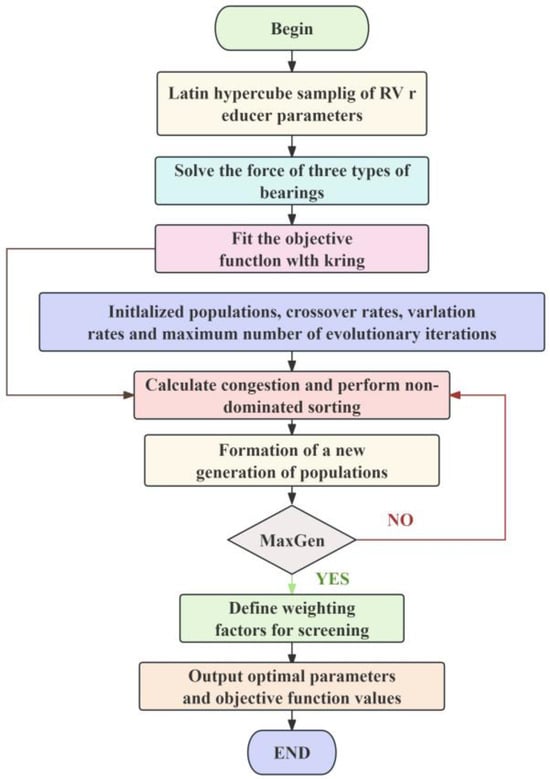
Figure 21.
Flowchart of the NSGA-II algorithm.
From the above analysis, it can be seen that a set of non-dominated optimized solutions is obtained after optimization by NSGA-II. In order to compare the degree of change in the objective function before and after optimization, it is necessary to define an evaluation function to assess the relative merits of the optimized solutions in the Pareto frontier set.
The optimization effect of each non-dominated solution of the Pareto frontier set is evaluated synthetically using the following equation [34].
The equivalent physical model of the main transmission chain system, which is constructed based on the spatial relationship between the main spindle bearing and various transmission components, is illustrated in Figure 8.
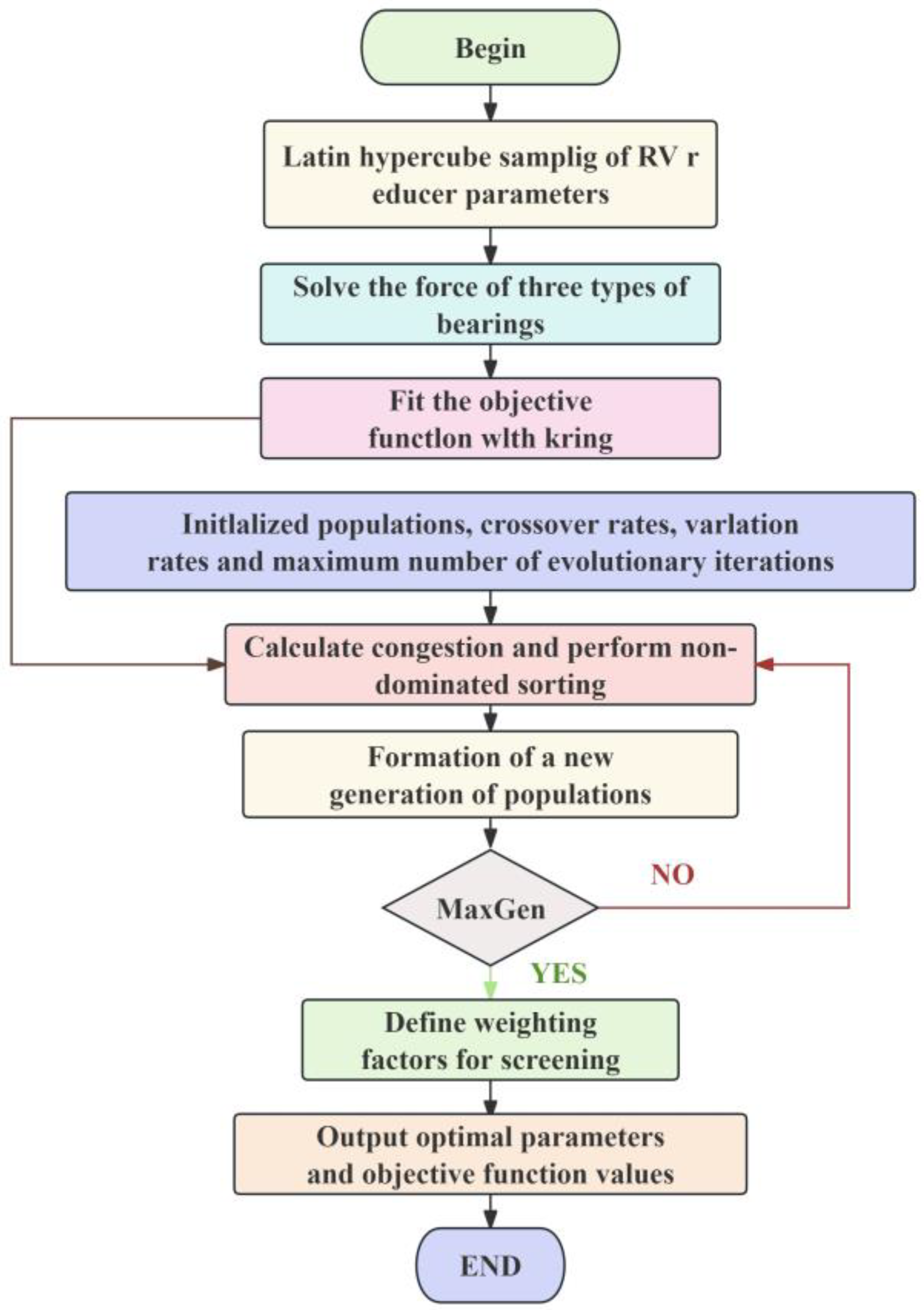
4.2.3. Solution Process
Based on the above analysis, the sample points are firstly determined using Latin hypercube sampling, and they are substituted into the mechanical model of the reducer bearing to be solved iteratively; then, the agent model of the objective function is established using the Kriging method, and this is combined with the NSGA-II algorithm to generate a set of Pareto frontier sets. Finally, the corresponding weights of the objective function are defined and substituted into the evaluation function to filter the optimal solution. The flowchart of the multi-objective optimization procedure for the crank support bearing, rotating arm bearing, and spindle bearing force is shown in Figure 22.
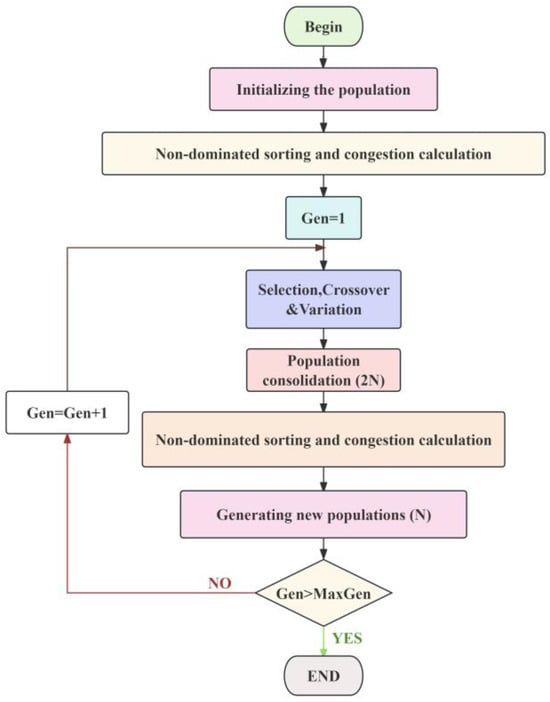
Figure 22.
Flowchart of Kriging-NSGA-II for the reducer shaft.
4.3. Optimization Results
4.3.1. Error Analysis of the Kriging Model
According to the operating parameters in Table 2 (using the rated operating conditions and taking the data when the input shaft rotation angle is 0), 60 sample points were selected through Latin hypercube sampling, and the complex correlation coefficient (R2) and root mean square error (RMSE) of the Kriging approximation model for the three types of shaft forces of the reducer are shown in Table 6; the fitting accuracy of the proxy model can be considered to have met the requirements if a complex correlation coefficient of is used. According to the results in Table 6, it can be seen that the established Kriging model is very reliable.
Table 6.
Error analysis of the Kriging model.
4.3.2. NSGA-II Algorithm Setup
For the NSGA-II algorithm, parameters such as population size, evolutionary generation, crossover rate, and variation rate have significant effects on the rationality of the Pareto frontier set distribution and the reliability of the final results. After continuous attempts, the population size is finally set to 100, the maximum evolutionary generation is set to 200, the variation rate is set to 0.1, and the crossover rate is set to 0.9.
According to the above study, it is found that the swivel arm shaft bearing force > crank support shaft bearing force > main shaft bearing force in the RV reducer; considering their different amplitudes, the bearing types, and the operating conditions, the Pareto frontier set weights for the crank support bearing, swivel arm bearing, and main bearing are finally taken as follows: , , and . The partly non-inferior dominated solution of the multi-objective optimization of the reducer shaft bearing force is shown in Figure 23:
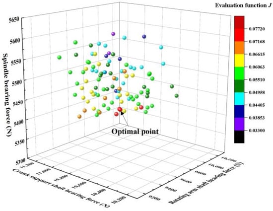
Figure 23.
Partially non-inferior dominant solution.
The structural parameters of the wheel bearing before and after optimization are obtained from the non-inferior dominated solutions in the figure, as shown in Table 7.
Table 7.
The RV reducer before and after optimization.
The table shows that the optimized crank support shaft load is reduced by 8.26%, the rotating arm shaft load is reduced by 10.35%, and the main shaft load is reduced by 5.15%. The optimization of the bearing load of the RV reducer is achieved.
5. Conclusions
This paper proposes a method for extracting the load spectra of RV reducers from both theoretical and simulation perspectives. The force analysis of the components of the RV reducer led to the derivation of force models for three shafts. By incorporating structural parameters and operating conditions, theoretical load spectra for the three shafts were calculated. Simulation analyses of the load spectra and structural parameters under different operating conditions were conducted, followed by structural optimization of the reducer, yielding the following results.
(1) The loads on the crank support bearing, swivel arm bearing, and main bearing all exhibit a sinusoidal trend. Among the three bearings, the swivel arm bearing experiences the highest load, followed by the crank support bearing, while the main bearing experiences the lowest load. The radial load on the main bearing varies periodically, with changes in load amplitude, while the axial load remains almost constant.
(2) As the output shaft torque increases, the load on all three bearings increases linearly. When the short amplitude coefficient increases, the loads on all three bearings initially increase. For the A360 RV reducer studied in this paper, the forces on all three shafts are minimized when the short amplitude coefficient is 0.786. As the eccentricity and transmission ratio increase, the forces on all three shafts decrease. As the needle tooth coefficient increases, the forces on all three shafts increase. The planetary wheel pressure angle and cycloid wheel width have little impact on the results.
(3) The simulated and theoretical calculation error for Condition II (rated operating condition) is 5.14%, with errors of 12.60% for the crank support bearing and 8.40% for the main bearing, which are relatively small errors. Both the theoretical calculations and simulation experiments verify the accuracy of the method in extracting the load spectra of RV reducer bearings.
(4) After structural optimization of the reducer, the load on the crank support bearing is reduced by 8.26%, the load on the swivel arm bearing is reduced by 10.35%, and the load on the main bearing is reduced by 5.15%.
This study accurately calculates the bearing stresses on the shafts of RV reducers and the response patterns and trends under different operating conditions. It also effectively optimizes the structure of the reducer, providing significant theoretical support for the high-precision and long-life design of internal bearings in high-precision RV reducers.
Author Contributions
Conceptualization, X.P. and D.Z.; methodology, X.P.; software, D.Z.; validation, D.Z. and X.W.; formal analysis, M.Y. and Q.L.; investigation, D.Z. and M.Y.; resources, Q.L. and M.Y.; data curation, X.P. and D.Z.; writing—original draft preparation, X.P. and D.Z.; writing—review and editing, X.P. and D.Z.; visualization, H.W. and D.L.; supervision, X.P.; project administration, X.P. and D.Z.; funding acquisition, Q.L. and D.L. All authors have read and agreed to the published version of the manuscript.
Funding
This work was supported by the National Key Research and Development Program of China (2020YFB2009603), the National Natural Science Foundation of China (52005159), and the National Natural Science Foundation of China (52205096).
Data Availability Statement
The data supporting the findings of this study are available from the corresponding author upon reasonable request. Due to the proprietary nature of some aspects of the research, particularly the detailed design parameters of the RV reducer and bearing configurations, not all data can be made publicly available. However, the key datasets, including the force analysis results, optimization parameters, and Kriging-NSGA-II algorithm implementation details, have been included within the article. Researchers interested in replicating or extending this work may contact the corresponding author for access to additional data, subject to confidentiality agreements where applicable.
Conflicts of Interest
Author Xinlong Wang was employed by the company Xinxiang Aviation Industry (Group) Co., Ltd. The remaining authors declare that the research was conducted in the absence of any commercial or financial relationships that could be construed as a potential conflict of interest.
Nomenclature
| Parameter | Name | Parameters | Name |
| Eccentricity distance | Number of planetary wheels | ||
| Number of cycloid wheels | Number of pinwheels | ||
| Rotation speed of part X | Transmission ratio of part M and part N with respect to part H | ||
| The force of part M on part N in the Z-direction | Force of part M on part N in the radial direction | ||
| Force of part M on part N in the tangent direction | The force of part M on part N in the vertical direction | ||
| Force of part M on part N with the changing direction | Planetary wheel pressure angle | ||
| Shift wheel pressure angle | Part X degree circle radius | ||
| Cycloid pinwheel output speed | Output load torque | ||
| Gravity of part X | Number of teeth in part X | ||
| Running corner of part X | Torque when the part X is running | ||
| The external force in the center of gravity of the needle and tooth shell | The bending moment of the center of gravity outside the needle shell | ||
| The Z-direction distance from the center of the part X to the coordinate origin | Cycloid wheel width | ||
| Tooth top height factor | Needle tooth coefficient | ||
| Evaluation function | Pre-optimization forces | ||
| Weighting factor of the force on the crank support shaft | Weighting factor of the force on the rotating arm shaft | ||
| Weighting factor of spindle bearing force | Regression coefficient | ||
| A flexible parameter that varies with the variables and can be obtained from the maximum likelihood estimation | Denotes the distance between sample points and for the variable | ||
| Approximate value of prediction points | Correlation matrix | ||
| Related vectors | Target value of the design point | ||
| Matrix of basis functions of design points | The generalized least square estimate of | ||
| True value of sample points | Predicted value of sample points | ||
| i | Planetary wheel ratio | K | Cycloid wheel short amplitude factor |
| θ | The crankshaft phase lag angle | δ | The short amplitude coefficient |
| e | Cycloid wheel eccentricity |
References
- Jiang, Z. Analysis of Dynamic Performance with RV Reducer. Master’s Thesis, Dalian Jiaotong University, Dalian, China, 2010; pp. 34–44. (In Chinese). [Google Scholar]
- Li, R. China’s industrial robot industrialization development strategy. Aeronaut. Manuf. Technol. 2010, 9, 32–37. (In Chinese) [Google Scholar]
- Salunkhe, V.; Khot, S.; Desavale, R.; Yelve, N. Unbalance Bearing Fault Identification Using Highly Accurate Hilbert—Huang Transform Approach. ASME J. Nondestruct. Eval. 2023, 6, 031005. [Google Scholar] [CrossRef]
- Peng, C. Test Technology and System Research of Robot Precision Reducer. Master’s Thesis, Chongqing University, Chongqing, China, 2020; pp. 31–36. (In Chinese). [Google Scholar]
- Yang, R.; Li, F.; Zhou, Y.; Xiang, J. Nonlinear dynamic analysis of a cycloidal ball planetary transmission considering tooth undercutting. Mech. Mach. Theory 2020, 145, 103694. [Google Scholar] [CrossRef]
- Wang, H.; Wang, L.; Su, J. Simulation analysis of transmission error of RV reducer based on ADAMS. Mach. Tool Hydraul. Press. 2021, 49, 135–140. (In Chinese) [Google Scholar]
- Tie, X.; Li, W.; Zhang, Z.; Jiao, C.; Xie, P.; Wang, C. Force analysis and life check of pendulum wheel bearing of RV reducer. Mech. Manuf. 2022, 60, 31–36. (In Chinese) [Google Scholar]
- Olejarczyk, K.; Wiko, M.; Koodziejczyk, K. The cycloidal gearbox efficiency for different types of bearings-sleeves vs. needle bearings. J. Mech. Eng. Sci. 2019, 233, 7401–7411. [Google Scholar] [CrossRef]
- Huang, J.; Li, C.; Chen, B. Optimization Design of RV Reducer Crankshaft Bearing. Appl. Sci. 2020, 10, 6520. [Google Scholar] [CrossRef]
- He, W.; Shan, L. Research and Analysis on Transmission Error of RV Reducer Used in Robot. Mech. Mach. Sci. 2015, 33, 231–238. [Google Scholar]
- Wu, S.; He, W.; Zhang, Y. Analysis of force and contact characteristics of rotating arm bearing for RV transmission mechanism. J. South China Univ. Technol. (Nat. Sci. Ed.) 2020, 48, 25–33. (In Chinese) [Google Scholar]
- Xu, L.; Yang, Y. Dynamic modeling and contact analysis of a cycloid-pin gear mechanism with a turning arm cylindrical roller bearing. Mech. Mach. Theory 2016, 104, 327–349. [Google Scholar] [CrossRef]
- Sun, Z.; Li, Y.; Wang, S.; Yang, D.; Li, F. Static simulation contact analysis of deep groove ball bearings based on ROMAX. J. Dalian Univ. 2019, 40, 21–26. (In Chinese) [Google Scholar]
- Guan, T.; Zhang, D. Study on the optimization design of antiarch profile in cycloid wheel. J. Mech. Eng. 2005, 41, 151–156. (In Chinese) [Google Scholar] [CrossRef]
- Yu, M.; Xu, C. Optimized design of cycloid pinwheel drive based on MATLAB. Mod. Manuf. Eng. 2010, 8, 141–143. (In Chinese) [Google Scholar]
- Liang, K.; Wang, Z.; Tian, S. Optimization Design and Simulation Analysis of Cycloid Pin Gear Planetary Reducer. J. Mech. Transm. 2017, 41, 155–159. (In Chinese) [Google Scholar]
- Wang, Y.; Qian, Q.; Chen, G. Multi objective optimization design of cycloid pin gear planetary reducer. Adv. Mech. Eng. 2017, 9, 1–10. [Google Scholar] [CrossRef]
- Wu, F.; Luo, J.; Zhang, L.; Wang, D. On the scope of application of Hertz point contact theory. Bearing 2007, 5, 1–3. (In Chinese) [Google Scholar] [CrossRef]
- Ye, X.; Wang, Q.; Chen, X. A Method for Force Analysis of an RV Reducer and a Device. CN Patent CN201811280759.4, 30 October 2018. (In Chinese). [Google Scholar]
- Yang, Q.; Wang, F.; He, L.; Tan, X.; Li, Y. Determination and optimization of the optimal short amplitude coefficient of the cycloid pinwheel planetary reducer. Appl. Technology. Lubr. 2010, 37, 1–4. (In Chinese) [Google Scholar] [CrossRef]
- Yang, R.; Han, B.; Xiang, J. Nonlinear Dynamic Analysis of a Trochoid Cam Gear with the Tooth Profile Modification. Int. J. Precis. Eng. Manuf. 2020, 21, 12. [Google Scholar] [CrossRef]
- Han, Z.; Wang, H.; Li, R.; Shan, W.; Zhao, Y.; Xu, H.; Tan, Q.; Liu, C.; Du, Y. Study on Nonlinear Dynamic Characteristics of RV Reducer Transmission System. Energies 2024, 17, 1178. [Google Scholar] [CrossRef]
- Zhang, Y.; Li, L.; Ji, S. The influence of the eccentricity of the cycloid wheel transmission mechanism on the bearing capacity. J. Harbin Eng. Univ. 2022, 143, 873–881. (In Chinese) [Google Scholar]
- Li, X. RV Transmission Pressure Angle Research and Parameter Optimization. Master’s Thesis, North China University of Technology, Beijing, China, 2021; pp. 8–14. (In Chinese). [Google Scholar]
- GB/T 10107.1-2012; Cycloid Pinwheel Planetary Transmission. Standards Press of China: Beijing, China, 2012. (In Chinese)
- Xu, L. Development of RV Reducer Digital Modeling Software and Optimization of Geometric Parameters. Master’s Thesis, Henan University of Science and Technology, Luoyang, China, 2022; pp. 15–21. (In Chinese). [Google Scholar]
- Song, S.; Yin, F. ADAMS Application in Mechanical Design; National Defense Industry Press: Beijing, China, 2015; pp. 122–124. (In Chinese) [Google Scholar]
- Feng, J.; Sun, Z.; Li, H.; Tian, Y. Optimization design method of bearing structure parameters based on Kriging model. J. Aerosp. Power 2017, 32, 723–729. (In Chinese) [Google Scholar]
- Bu, J.; Zhou, M.; Lan, X.; Lv, K. Optimization for Airgap Flux Density Waveform of Flywheel Motor Using NSGA-2 and Kriging Model Based on MaxPro Design. IEEE Trans. Magn. 2017, 53, 8. [Google Scholar] [CrossRef]
- Jeong, S.; Murayama, M.; Yamamoto, K. Efficient Optimization Design Method Using Kriging Model. J. Aircr. 2005, 42, 2. [Google Scholar] [CrossRef]
- Salunkhe, V.; Desavale, R.; Jagadeesha, T. Experimental Frequency-Domain Vibration Based Fault Diagnosis of Roller Element Bearings Using Support Vector Machine. ASME J. Risk Uncertain. Part B 2021, 7, 021001. [Google Scholar] [CrossRef]
- Hua, Y.; Liu, Y.; Pan, W.; Diao, X.; Zhu, H. Multi-objective optimization design of bearing-free permanent magnet synchronous motor based on improved particle swarm algorithm. Chin. J. Electr. Eng. 2023, 43, 1–9. (In Chinese) [Google Scholar] [CrossRef]
- Hu, J.; Zhai, J.; Zhang, X.; Li, H.; Xun, B. Optimal structural design of two-stage series bearings based on response surface method. J. Mil. Eng. 2022, 43, 694–703. (In Chinese) [Google Scholar]
- Salunkhe, V.; Desavale, R.; Khot, S.; Yelve, N. Identification of Bearing Clearance in Sugar Centrifuge Using Dimension Theory and Support Vector Machine on Vibration Measurement. ASME J. Nondestruct. Eval. 2024, 7, 021003. [Google Scholar] [CrossRef]

Disclaimer/Publisher’s Note: The statements, opinions and data contained in all publications are solely those of the individual author(s) and contributor(s) and not of MDPI and/or the editor(s). MDPI and/or the editor(s) disclaim responsibility for any injury to people or property resulting from any ideas, methods, instructions or products referred to in the content. |
© 2025 by the authors. Licensee MDPI, Basel, Switzerland. This article is an open access article distributed under the terms and conditions of the Creative Commons Attribution (CC BY) license (https://creativecommons.org/licenses/by/4.0/).