An Experimentally Validated Cavitation Model for Hydrodynamic Bearings Using Non-Condensable Gas


 ,
,  ,
,  ,
, 
Abstract

1. Introduction
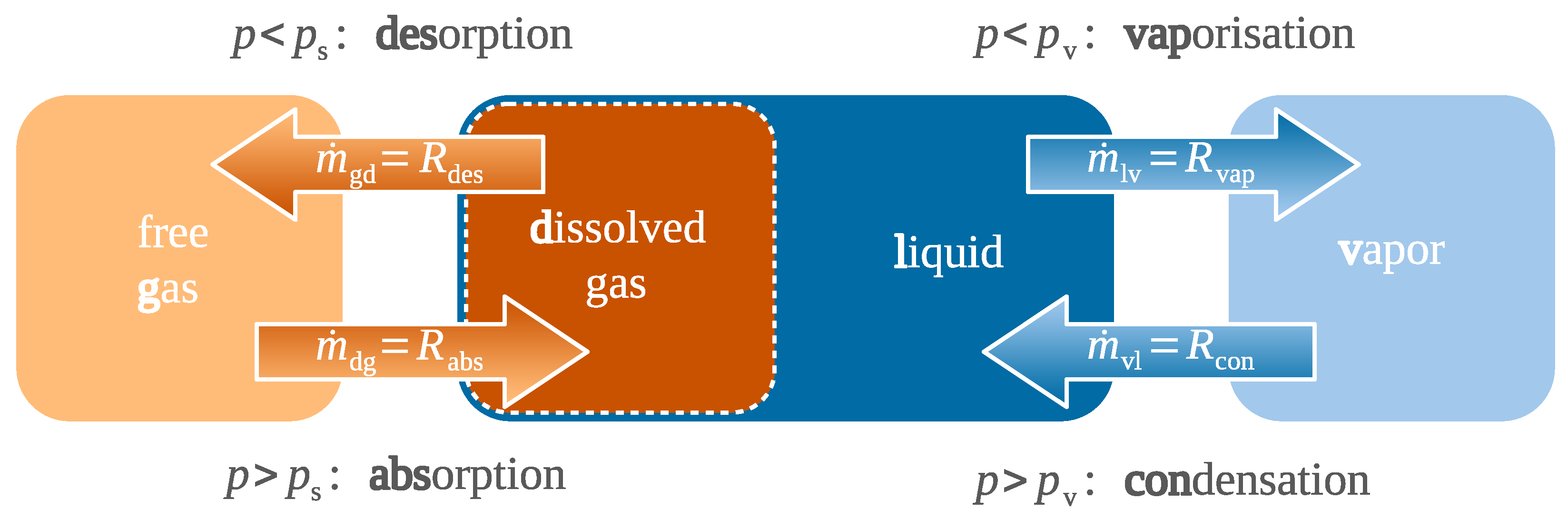
- Vaporous cavitation occurs when the pressure falls below the vapor pressure of the liquid phase and boiling begins. Depending on the temperature, Ref. [1] gives values for the vapor pressure of typical oil mixture components between and that are close to the vacuum.
- Gaseous cavitation is caused by dissolved gas that will be desorbed when pressure drops below saturation pressure. Braun and Hannon provide values for the temperature-dependent saturation pressure of between and .
- Pseudo-cavitation is a special case of gaseous cavitation when the gas is completely undissolved. This type of cavitation is caused by the expansion of dispersed gas bubbles due to depressurization. The processes of molecular dissolution and absorption do not occur, and the total amount of free gas is constant (). The gas can enter the system either via the lubricant or directly from the environment.
2. Mathematical Model
2.1. Governing Equations
2.2. Material Laws
2.3. Numerical Solution
3. Test Case
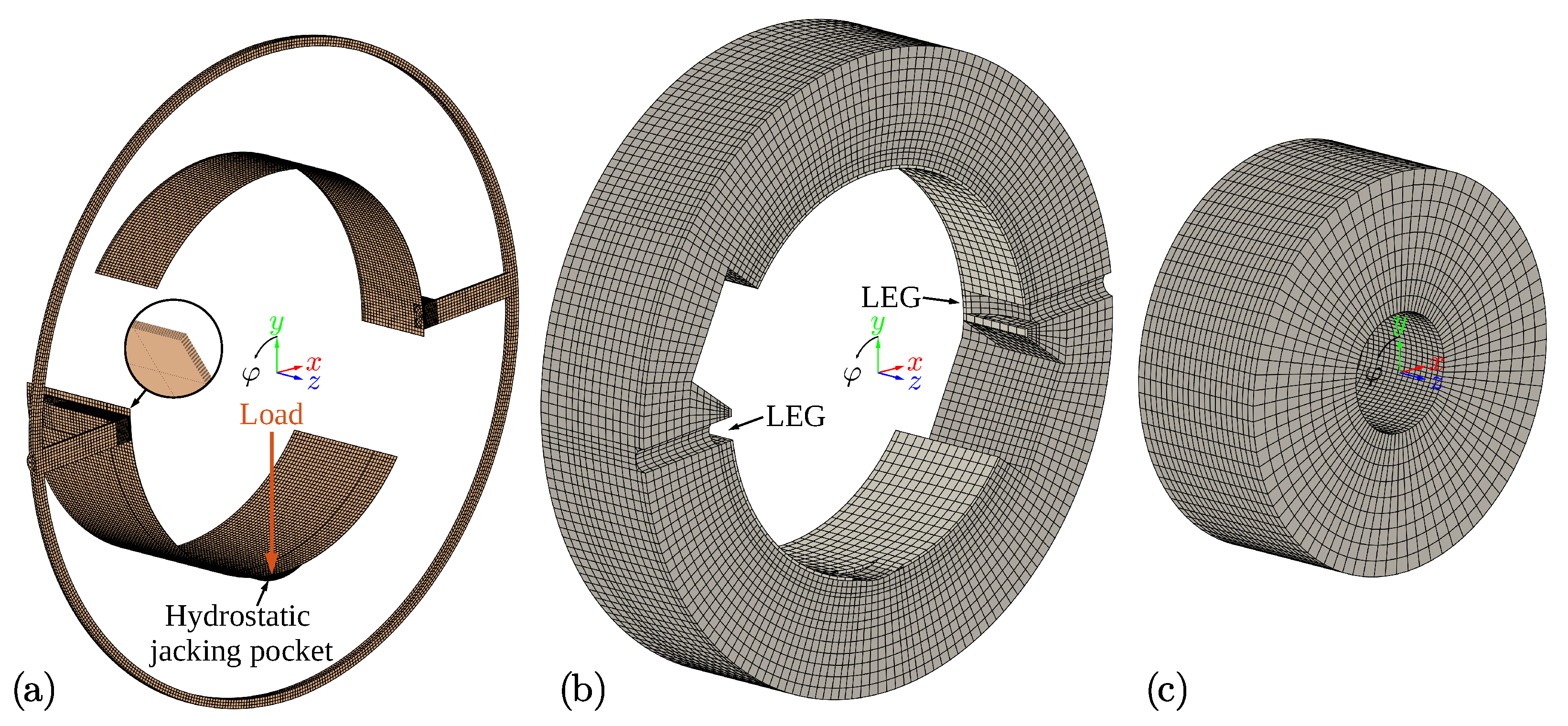
3.1. Geometry
3.2. Material Parameters
3.3. Boundary Conditions
4. Numerical Results
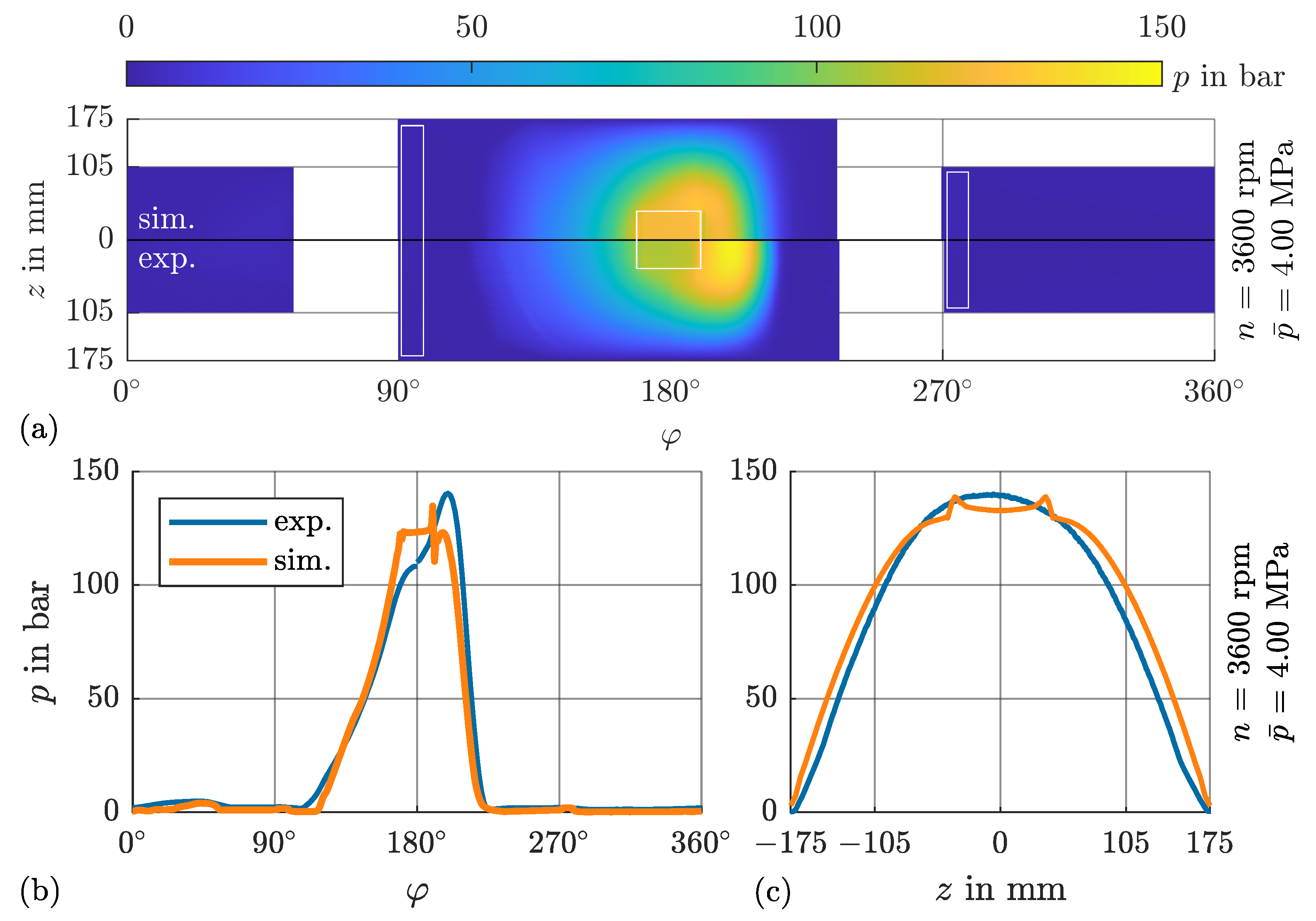
4.1. Pressure
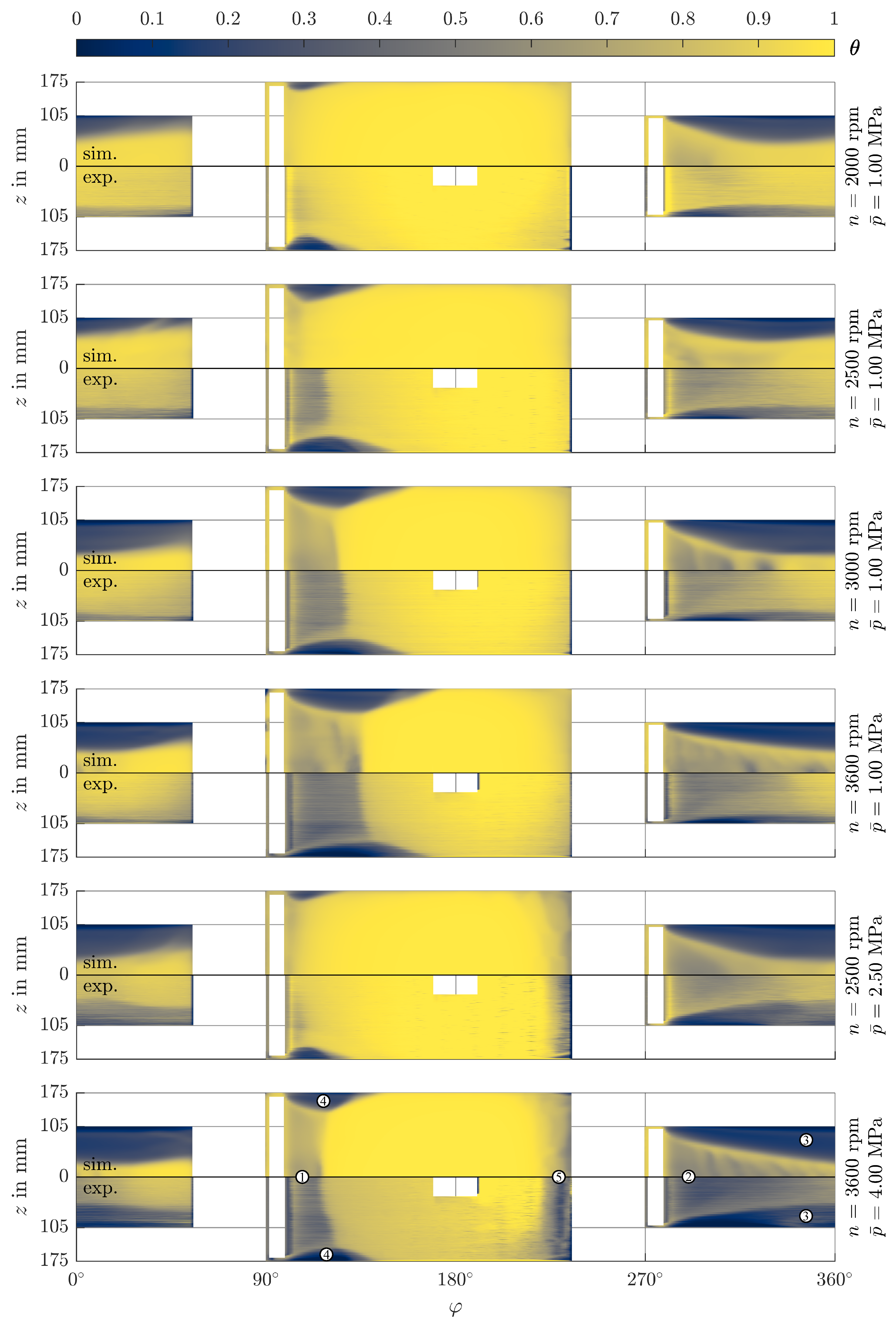
4.2. Volume Fraction and Fractional Film Content
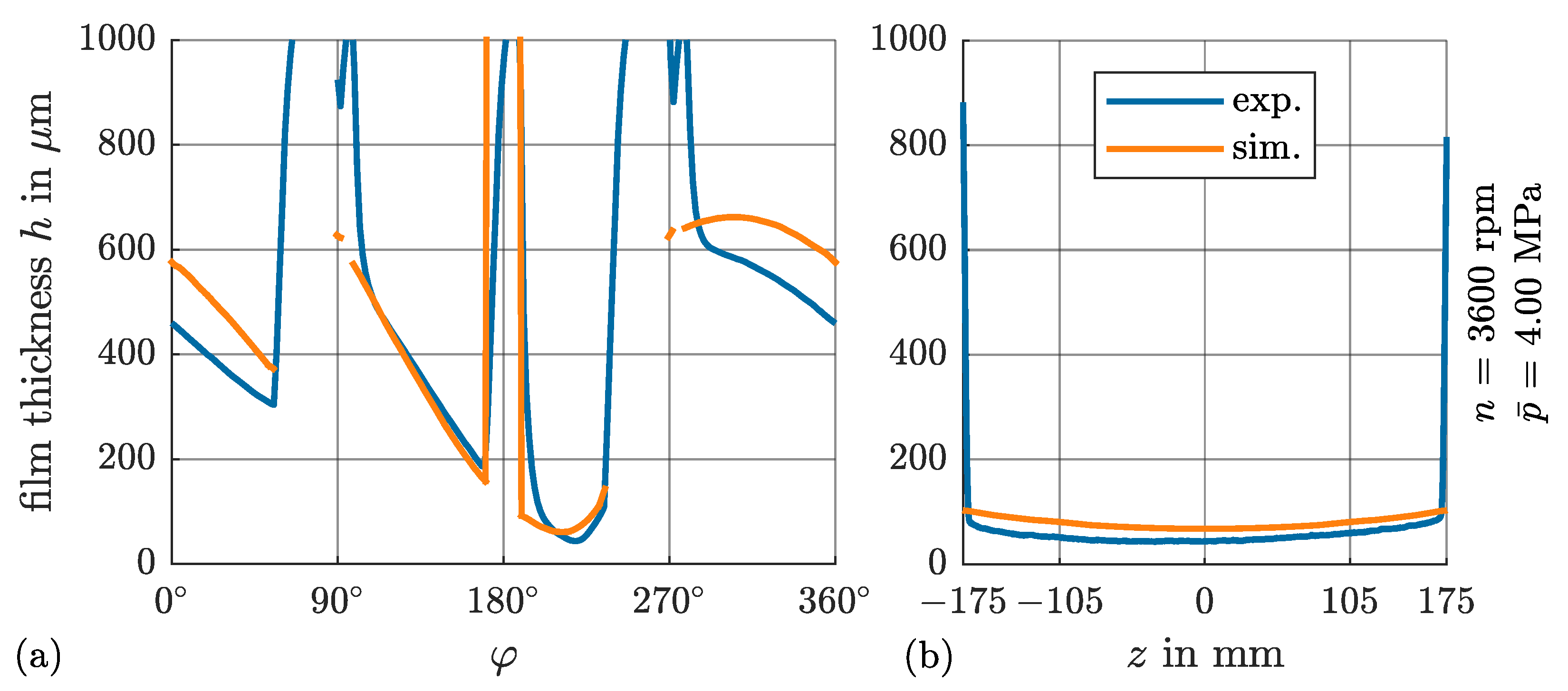
4.3. Film Thickness
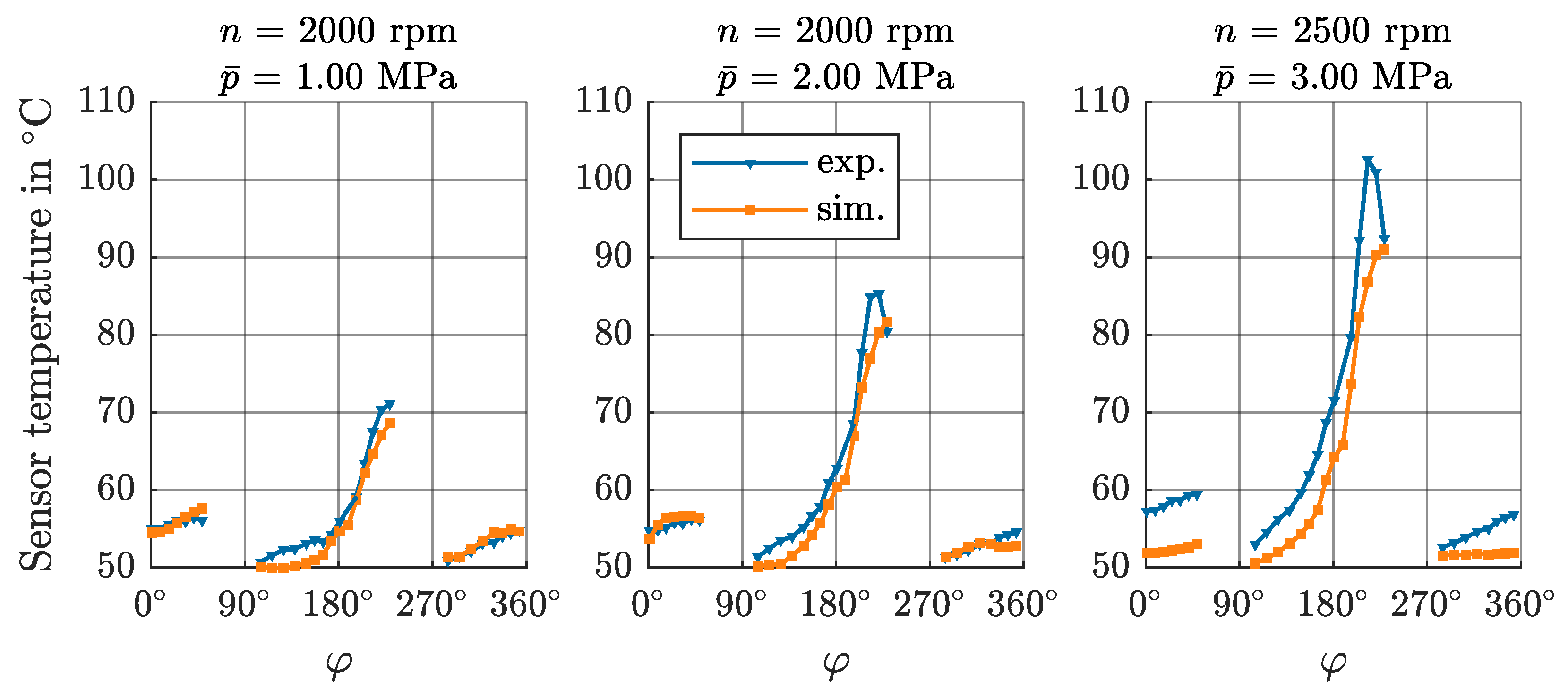
4.4. Temperature
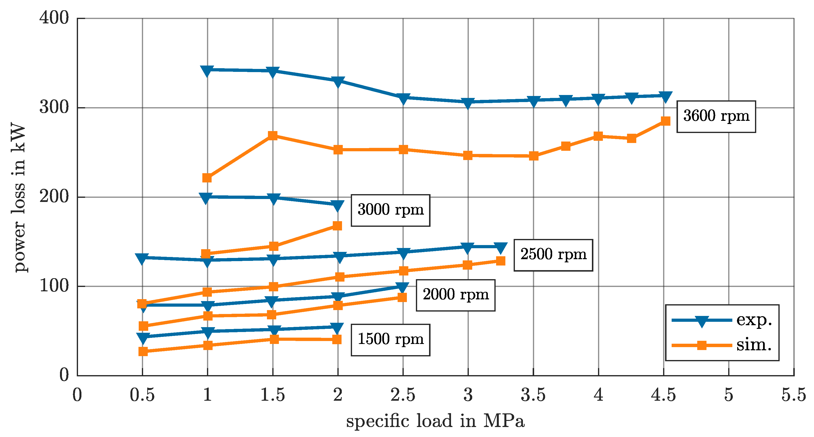
4.5. Power Loss
4.6. Effect of the Bunsen Solubility Coefficient
5. Conclusions
Author Contributions
Funding
Data Availability Statement
Conflicts of Interest
Nomenclature
| Latin Symbols | Greek Symbols | ||
| a | Thermal expansion rate | Bunsen solubility coefficient | |
| Specific heat at constant pressure | Compressibility factor | ||
| E | Young’s modulus | Deformation tensor | |
| h | Film thickness, static enthalpy | Dynamic viscosity | |
| External field | Fractional film content | ||
| l | Falz exponent | Heat conductivity | |
| Mass transfer rate from phase to | Poisson’s ratio | ||
| n | Rotational speed | Density | |
| p | Absolute pressure | Cauchy stress tensor | |
| Cavitation pressure | Viscous stress tensor | ||
| Saturation pressure | Dissipation term | ||
| Vapor pressure | Circumferencial angle | ||
| Specific load | Integration domain | ||
| R | Gas constant | Boundary of | |
| Absorption rate | |||
| Condensation rate | Operators | ||
| Desorption rate | Frobenius scalar product | ||
| Vaporisation rate | Dot product | ||
| r | Volume fraction | Gradient | |
| t | Time | Divergence | |
| External stress | Dyadic product | ||
| T | Temperature | Deviator | |
| Surface velocity | Trace | ||
| Solid displacement | Transposition | ||
| V | Volume | ||
| Fluid velocity | Subscripts | ||
| Spacial coordinates | Gas | ||
| Liquid | |||
| Vapor | |||
| Reference value | |||
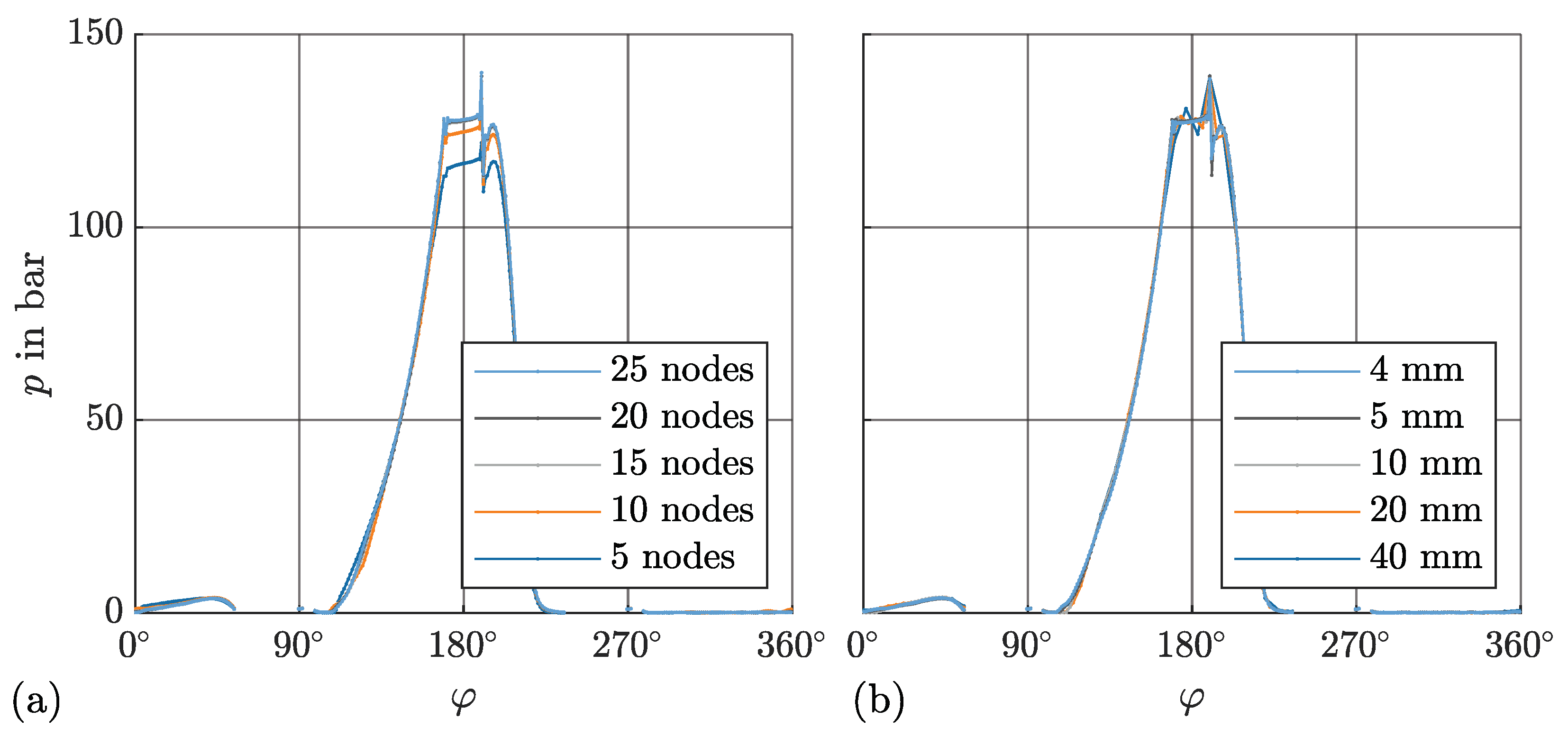
Appendix A. Mesh Independency Study
References
- Braun, M.J.; Hannon, W.M. Cavitation formation and modeling for fluid film bearings: A review. Proc. Inst. Mech. Eng. Part J J. Eng. Tribol. 2010, 224, 839–863. [Google Scholar] [CrossRef]
- Elrod, H.G. A cavitation algorithm. J. Lubr. Technol. 1981, 103, 350–354. [Google Scholar] [CrossRef]
- Schnerr, G.; Sauer, J. Physical and Numerical Modeling of Unsteady Cavitation Dynamics. In Proceedings of the 4th International Conference on Multiphase Flow, New Orleans, LA, USA, 27 May–1 June 2001. [Google Scholar]
- Singhal, A. Mathematical Basis and Validation of the Full Cavitation Model. J. Fluids Eng. 2002, 124, 617–624. [Google Scholar] [CrossRef]
- Zwart, P.; Gerber, A.G.; Belamri, T. A two-phase flow model for predicting cavitation dynamics. In Proceedings of the ICMF 2004 International Conference on Multiphase Flow, Yokohama, Japan, 30 May–3 June 2004. [Google Scholar]
- Peeken, H.; Benner, J. Beeinträchtigung des Druckaufbaus in Gleitlagern durch Schmierstoffverschäumung. VDI-Berichte 1985, 549, 373–397. [Google Scholar]
- Li, X.; Song, Y.; Hao, Z.; Gu, C. Cavitation Mechanism of Oil-Film Bearing and Development of a New Gaseous Cavitation Model Based on Air Solubility. J. Tribol. 2012, 134, 31701. [Google Scholar] [CrossRef]
- Hao, Z.; Gu, C. Numerical modeling for gaseous cavitation of oil film and non-equilibrium dissolution effects in thrust bearings. Tribol. Int. 2014, 78, 14–26. [Google Scholar] [CrossRef]
- Song, Y.; Gu, C.; Ren, X. Development and validation of a gaseous cavitation model for hydrodynamic lubrication. Proc. Inst. Mech. Eng. Part J J. Eng. Tribol. 2015, 2299, 1227–1238. [Google Scholar] [CrossRef]
- Ding, A.; Li, X.; Li, Y. Improvement and analysis for a gaseous cavitation model applied in a tilting pad journal bearing. In Proceedings of the ASME Turbo Expo 2019: Turbomachinery Technical Conference and Exposition, Phoenix, AZ, USA, 17–21 June 2019; Volume 7B: Structures and Dynamics. [Google Scholar] [CrossRef]
- Ding, A.; Ren, X.; Li, X.; Gu, C. A new gaseous cavitation model in a tilting-pad journal bearing. Sci. Prog. 2021, 104, 368504211029431. [Google Scholar] [CrossRef] [PubMed]
- Ibata, Y.; Matsuura, Y.; Takahashi, S.; Iga, Y. Development of gaseous cavitation model in hydraulic oil flow considering the effect of dynamic stimulation. IOP Conf. Ser. Earth Environ. Sci. 2019, 240, 62041. [Google Scholar] [CrossRef]
- Osterland, S.; Günther, L.; Weber, J. Experiments and CFD on vapor and gas cavitation for oil hydraulics. Chem. Eng. Technol. 2022, 46, 147–157. [Google Scholar] [CrossRef]
- Reinke, P.; Ahlrichs, J.; Beckmann, T.; Schmidt, M. High-Speed Digital Photography of Gaseous Cavitation in a Narrow Gap Flow. Fluids 2022, 7, 159. [Google Scholar] [CrossRef]
- Hagemann, T.; Vetter, D.; Wettmarshausen, S.; Stottrop, M.; Engels, A.; Weißbacher, C.; Bender, B.; Schwarze, H. A Design for High-Speed Journal Bearings with Reduced Pad Size and Improved Efficiency. Lubricants 2022, 10, 313. [Google Scholar] [CrossRef]
- Engels, A.; Wettmarshausen, S.; Stottrop, M.; Hagemann, T.; Weißbacher, C.; Schwarze, H.; Bender, B. Experimental Identification of the Void Fraction in a Large Hydrodynamic Offset Halves Bearing. Lubricants 2024, 13, 7. [Google Scholar] [CrossRef]
- Dowson, D.; Godet, M.; Taylor, C.M. Cavitation and Related Phenomena in Lubrication: Proceedings of the 1st Leeds-Lyon Symposium on Tribology, Held in The Institute of Tribology, Department of Mechanical Engineering, The University of Leeds, England, September 1974; Mechanical Engineering Publications Limited: London, UK, 1975. [Google Scholar]
- Menter, F.R. Two-Equation Eddy-Viscosity Turbulence Models for Engineering Applications. AIAA J. 1994, 32, 1598–1605. [Google Scholar] [CrossRef]
- Langtry, R.B. A Correlation-Based Transition Model Using Local Variables for Unstructured Parallelized CFD Codes. Doctoral Dissertation, Universität Stuttgart, Fakultät Energie, Verfahrens und Biotechnik, Stuttgart, Germany, 2006. [Google Scholar] [CrossRef]
- Falz, E. Grundzüge der Schmiertechnik, 2nd ed.; Springer: Berlin/Heidelberg, Germany, 1931. [Google Scholar]
- Hagemann, T.; Zeh, C.; Prölß, M.; Schwarze, H. The Impact of Convective Fluid Inertia Forces on Operation of Tilting-Pad Journal Bearings. Int. J. Rotating Mach. 2017, 2017, 5683763. [Google Scholar] [CrossRef]


| Parameter | Nominal | Measured | Unit |
|---|---|---|---|
| Rel. bearing clearance | ‰ | ||
| Preload unloaded pad | |||
| Preload loaded pad | |||
| Angle of curvature center of unloaded pad | |||
| Angle of curvature center of loaded pad | |||
| Bore diameter | |||
| Pad radius | |||
| Outer diameter | 800 | ||
| Width unloaded pad | 350 | ||
| Width loaded pad | 210 | ||
| Shaft outer diameter | |||
| Shaft inner diameter | 150 |
| Parameter | Steel | White Metal | Unit |
|---|---|---|---|
| Density | 7870 | 7400 | |
| Young’s modulus E | |||
| Poisson’s ratio | 0.28 | 0.33 | 1 |
| Thermal expansion rate a | 1 | ||
| Specific heat | 440 | 230 | |
| Heat conductivity | 35 |
| Parameter | Value | Unit | ||||||
|---|---|---|---|---|---|---|---|---|
| Temperature T | 20 | 40 | 60 | 80 | 100 | 120 | 140 | |
| Density | ||||||||
| Dynamic viscosity | ||||||||
| Specific heat | ||||||||
| Heat conductivity | ||||||||
Disclaimer/Publisher’s Note: The statements, opinions and data contained in all publications are solely those of the individual author(s) and contributor(s) and not of MDPI and/or the editor(s). MDPI and/or the editor(s) disclaim responsibility for any injury to people or property resulting from any ideas, methods, instructions or products referred to in the content. |
© 2025 by the authors. Licensee MDPI, Basel, Switzerland. This article is an open access article distributed under the terms and conditions of the Creative Commons Attribution (CC BY) license (https://creativecommons.org/licenses/by/4.0/).
Share and Cite
Wettmarshausen, S.; Engels, A.; Hagemann, T.; Stottrop, M.; Weißbacher, C.; Schwarze, H.; Bender, B. An Experimentally Validated Cavitation Model for Hydrodynamic Bearings Using Non-Condensable Gas. Lubricants 2025, 13, 140. https://doi.org/10.3390/lubricants13040140
Wettmarshausen S, Engels A, Hagemann T, Stottrop M, Weißbacher C, Schwarze H, Bender B. An Experimentally Validated Cavitation Model for Hydrodynamic Bearings Using Non-Condensable Gas. Lubricants. 2025; 13(4):140. https://doi.org/10.3390/lubricants13040140
Chicago/Turabian StyleWettmarshausen, Sören, Alexander Engels, Thomas Hagemann, Michael Stottrop, Christoph Weißbacher, Hubert Schwarze, and Beate Bender. 2025. "An Experimentally Validated Cavitation Model for Hydrodynamic Bearings Using Non-Condensable Gas" Lubricants 13, no. 4: 140. https://doi.org/10.3390/lubricants13040140
APA StyleWettmarshausen, S., Engels, A., Hagemann, T., Stottrop, M., Weißbacher, C., Schwarze, H., & Bender, B. (2025). An Experimentally Validated Cavitation Model for Hydrodynamic Bearings Using Non-Condensable Gas. Lubricants, 13(4), 140. https://doi.org/10.3390/lubricants13040140