Abstract
(1) Background: Rolling bearings are important components in mechanical equipment, but they are also components with a high failure rate. Once a malfunction occurs, it will cause mechanical equipment to malfunction and may even affect personnel safety. Therefore, studying the fault diagnosis methods for rolling bearings is of great significance and is also a current research hotspot and frontier. However, the vibration signals of rolling bearings usually exhibit nonlinear and non-stationary characteristics, and are easily affected by industrial environmental noise, making it difficult to accurately diagnose bearing faults. (2) Methods: Therefore, this article proposes a rolling bearing fault diagnosis model based on an improved dung beetle optimizer (DBO) algorithm-optimized variational mode decomposition-convolutional neural network-bidirectional long short-term memory (VMD-CNN-BiLSTM). Firstly, an improved DBO algorithm named CSADBO is proposed by integrating multiple strategies such as chaotic mapping and cooperative search. Secondly, the optimal parameter combination of VMD was adaptively determined through the CSADBO algorithm, and the optimized VMD algorithm was used to perform modal decomposition on the bearing vibration signal. Then, CNN-BiLSTM was used as the model for fault classification, and hyperparameters of the model were optimized using the CSADBO algorithm. (3) Results: Finally, multiple experiments were conducted on the bearing dataset of Case Western Reserve University, and the proposed method achieved an average diagnostic accuracy of 99.6%. (4) Conclusions: Experimental comparisons were made with other models to verify the effectiveness of the proposed model. The experimental results show that the proposed model based on an improved DBO algorithm optimized VMD-CNN-BiLSTM can effectively be used for rolling bearing fault diagnosis, with high diagnostic accuracy, and can provide a theoretical reference for other related fault diagnosis problems.
1. Introduction
As one of the core components of rotating machinery, rolling bearings are widely used in industrial production. Rolling bearings play a role in transmission and support in rotating machinery, and their health status directly affects the performance and lifespan of mechanical equipment [1]. But due to the long-term operation of mechanical equipment under harsh and complex working conditions, the failure rate of rolling bearings is high. Once rolling bearings fail, it will lead to the inability of mechanical equipment to operate normally, and, in severe cases, it may even cause major accidents [2]. According to statistics, approximately 45% to 55% of rotating machinery failures are related to damage to rolling bearings [3]. It can be seen that, if rolling bearing faults can be identified and eliminated in a timely manner during the production process, it will greatly reduce the probability of equipment failure and reduce the later maintenance cost of the equipment. Therefore, studying how to efficiently and accurately detect rolling bearing faults is of great practical significance.
Due to the environmental impact on bearings during the overall operation of mechanical equipment systems, and the non-stationary and nonlinear characteristics of bearing vibration signals, they are easily affected by noise interference, making it difficult to extract important features of vibration signals. Therefore, in order to solve the problem of signal feature extraction, many scholars have studied signal processing methods and applied them in the field of fault diagnosis. X. Song et al. [4] used the empirical mode decomposition (EMD) algorithm to decompose the original bearing fault signal into multiple modal components, and extracted the time–frequency domain features of the signal to construct a feature matrix. D. Meng et al. [5] analyzed the natural frequency and characteristic frequency of bearing fault signals, and extracted the features of fault signals based on the EMD algorithm. L. Zhang et al. [6] extracted early weak fault features of bearings based on the local mean decomposition (LMD) algorithm. Although the above methods can extract fault signal features, the decomposed signal components are prone to endpoint effects and mode aliasing problems. Dragomiretskiy et al. [7] innovatively described the variational mode decomposition (VMD) algorithm, which constructs a constrained variational model and transforms signal decomposition into the problem of finding the optimal solution of the variational model. This can effectively solve the problems of endpoint effects and mode mixing. Therefore, since the VMD algorithm was proposed, it has been widely used in the field of fault diagnosis. D. Huang et al. [8] compared the effectiveness of LMD and VMD algorithms in decomposing fault signals and verified through experiments that the VMD algorithm has better decomposition performance. L. Fu et al. [9] used the VMD algorithm to decompose the fault signal and extracted important features from the results of VMD using the principal component analysis (PCA) method. However, the VMD algorithm also has certain shortcomings. C. Liu et al. [10] believe that, although the VMD algorithm performs better in extracting fault features than other decomposition algorithms, the number of modal decompositions K and the penalty factor in the algorithm will have a significant impact on the final decomposition result. Therefore, setting the parameters in the VMD algorithm reasonably is of great significance. S. Chen et al. [11] described a VMD parameter optimization method based on dung beetle optimizer (DBO) to seek the optimal parameter combination. S. Tan et al. [12] used the cuckoo search algorithm to effectively extract the fault characteristics of bearings and obtain the optimal parameters of VMD, thereby decomposing the fault signal into a set of optimal components. M. Wang et al. [13] optimized VMD parameters based on the sparrow search algorithm and combined them with support vector machine (SVM) to diagnose bearing fault signals, achieving good results. Z. Wang et al. [14] described an improved DBO algorithm that enhances the global search ability and applied it to optimize the VMD algorithm. Experimental results have shown that the optimized VMD algorithm can effectively perform modal decomposition on fault signals.
In researching fault diagnosis methods for rolling bearings, D. Dou et al. [15] described a rule-based fault diagnosis method and validated it on a bearing vibration dataset, which can effectively diagnose bearing faults. However, traditional rule-based methods also have certain limitations in bearing fault diagnosis, such as difficulty in handling complex nonlinear data. The emergence of machine learning and deep learning technologies has provided new solutions to overcome the limitations of traditional rule-based methods. Therefore, applying intelligent algorithm models to the field of bearing fault diagnosis has gradually become a research hotspot for scholars at home and abroad. X. Liu et al. [16] applied convolutional neural networks to fault diagnosis tasks, learning and extracting features from a large amount of bearing vibration data through convolutional neural networks, thereby achieving high fault diagnosis accuracy. B. Liu et al. [17] first used a VMD algorithm to decompose the fault signal of rolling bearings, and then recognized extracted fault features through a probabilistic neural network (PNN) to achieve fault classification. L. Eren et al. [18] described a fault diagnosis method based on a 1D convolutional neural network (1D CNN) and tested the method on the Case Western Reserve University (CWRU) bearing dataset, achieving good diagnostic results. H. Pan et al. [19] combined a CNN and LSTM to form a bearing fault diagnosis model and demonstrated the effectiveness of the proposed model through experiments. D. Zhao et al. [20] pointed out that, under variable speed conditions, rotational frequency (RF) is a key factor in determining whether rolling bearing faults occur. D. Zhao et al. [21] described a frequency matching demodulation transform technique that accurately captures the fault characteristics of rolling bearings and has achieved excellent experimental results. L. Cui et al. [22] described a rolling bearing remaining useful life prediction model based on an improved particle filtering algorithm, achieving excellent predictive performance. D. Zhao et al. [23] described how the FCSSCT method is able to effectively capture the characteristic representation of fault signals. Y. Da et al. [24] proposed a bearing fault diagnosis method based on CNN-BiLSTM, which has better generalization performance. However, the selection of hyperparameters in intelligent algorithm models has a significant impact on the performance of the model. Therefore, setting hyperparameters reasonably can effectively improve the accuracy of the model in identifying bearing faults. In order to improve the accuracy of fault diagnosis, T. He et al. [25] used an improved particle swarm optimization (PSO) algorithm to optimize the hyperparameters of the CNN-LSTM network model, and demonstrated the superiority of the proposed method through comparative experiments. B. Song et al. [26] described a method to optimize the hyperparameters of the CNN-BiLSTM model through an improved PSO algorithm, and used the optimized CNN-BiLSTM model to complete the task of bearing fault diagnosis, which can effectively classify fault signals. C. Zhang et al. [27] described a fault diagnosis model based on an improved PNN, using the improved DBO algorithm to optimize the smoothing factor of the PNN, thereby improving the accuracy of fault classification. The optimization algorithm can adaptively find the optimal parameters of the model, but heuristic algorithms are prone to becoming stuck in local optima during the iterative optimization process.
Combining the above analyses, it can be seen that, although the VMD algorithm is able to solve the endpoint effect and modal overlap problems better, the effectiveness of its decomposition is greatly affected by the number of decomposition layers K and the penalty factor . Neural network models are widely used in the field of bearing fault diagnosis, but their performance is largely limited by the selection of hyperparameters. Although the use of heuristic algorithms for adaptive optimization provides a new approach to solving hyperparameter selection problems, special attention should also be paid to the problem of heuristic algorithms easily falling into local optima. To address the aforementioned issues, this paper proposes a rolling bearing fault diagnosis method based on an improved DBO algorithm optimized VMD-CNN-BiLSTM model. The research is summarized below:
- (1)
- An improved DBO algorithm (CSADBO) with embedded chaotic mapping, cooperative search, and an adaptive t-distribution strategy was proposed, which greatly improved the optimization ability and convergence speed of the algorithm and effectively solved the problem of local optimal solutions.
- (2)
- A parameter optimization method based on the CSADBO algorithm for VMD and CNN-BiLSTM was proposed, and the optimal parameter combination in the VMD algorithm was determined. A set of hyperparameters of the CNN-BiLSTM network model was optimized, and the model incorporating the optimal parameters was successfully applied to the fault diagnosis task of rolling bearings.
- (3)
- The model described in this paper was tested on the CWRU dataset and compared with several other fault diagnosis models. The experimental results showed that the model proposed in this paper has high diagnostic accuracy and excellent performance compared to other models.
The remaining parts of this paper are organized as follows: The second part describes relevant theories and technologies needed in this article, providing theoretical support for the improvement of subsequent algorithms and models. The third part elaborates in detail on the parameter optimization method based on the improved DBO algorithm. The fourth part introduces a rolling bearing fault diagnosis model based on CSADBO-VMD-CNN-BiLSTM, and elaborates on the implementation process of the model in detail. The fifth part conducted simulation experiments to evaluate and analyze the performance of the algorithm and model. The sixth part is the conclusion.
2. Related Theories and Technologies
2.1. Convolutional Neural Network
Convolutional neural networks can delve deep into the intrinsic relationships between data and effectively extract deep features [28]. A one-dimensional CNN has the advantages of low computational complexity and a large receptive field, making it widely used for tasks involving processing time series information [29]. The collected bearing dataset is usually time series data, so this article uses a 1D CNN to process fault signal data. Firstly, one-dimensional fault signal data are convolved through convolutional layers, and then nonlinear activation and pooling operations are performed to obtain more representative feature representations of the input signal.
Here, the convolutional layer is an important component of the CNN. The formula is shown in Formula (1).
where b is the bias parameter and represents the weight matrix; x represents the feature result of the convolution output; is the activation function. Commonly used activation functions include ReLU, Sigmoid, etc. Due to its fast convergence and non-saturation properties, this paper selects the ReLU function as the activation function, as shown in Formula (2).
The pooling layer’s function is to downsample the input data. In this paper, the max pooling method was chosen, as shown in Formula (3).
where s is the width of pooling; indicates the activation value; indicates the k-th output value of the j-th neuron in the l-th layer after the pooling operation.
2.2. Bidirectional Long Short-Term Memory Neural Network
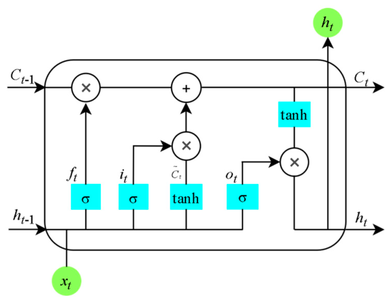
The long short-term memory (LSTM) neural network is an improvement on the recurrent neural network (RNN), aimed at solving the problems of gradient vanishing and exploding in the traditional RNN for long sequence modeling [30]. The structure of LSTM is shown in Figure 1.
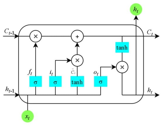
Figure 1.
LSTM structure.
The function of the forget gate is to discard or retain some unit information from the previous layer with a certain probability; the input gate is responsible for selectively updating input information; the output gate is responsible for controlling the data that the current unit needs to output. The specific calculation is shown in Formula (4).
Among them, , , and indicate outputs of the forget gate, input gate, and output gate, respectively; and tanh represent the activation functions; , , , and are weight coefficient matrices of the corresponding gates, respectively; , , , and are the bias vectors of the corresponding gates; and , respectively, represent the output and information status of this unit.
Although LSTM can effectively model time series data, it only considers forward time series when processing data and fails to pay attention to the impact of reverse time series data on the model. Bidirectional long short-term memory (BiLSTM) neural networks can obtain more contextual data through forward and backward propagation, thereby improving the understanding and modeling ability of time series data. Compared with unidirectional LSTM, its feature representation is more comprehensive and rich. Figure 2 illustrates the architecture of BiLSTM.
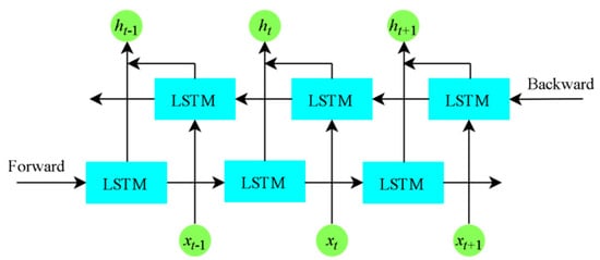
Figure 2.
BiLSTM structure.
After extracting key temporal features through BiLSTM, this paper adds a fully connected layer after the BiLSTM layer to integrate these features, and uses the Softmax activation function to map the extracted features to probability distributions of different categories. The expression is shown in Formula (5).
where represents the probability after Softmax; represents the output value of the i-th neuron; N is the number of categories classified.
2.3. Variational Mode Decomposition
The Variational Mode Decomposition (VMD) algorithm was proposed by Dragomiretskiy et al. [7] in 2014. This algorithm can iteratively search and decompose the original complex signal into K intrinsic mode functions (IMF) with different frequencies and bandwidths. The implementation process of the VMD algorithm mainly involves constructing and solving variational problems.
- (1)
- Construction of variational problems:
Assuming that K IMF components are obtained after decomposition by the VMD algorithm, they are redefined as the modal function with a finite bandwidth, as shown in Formula (6).
The analytical signal corresponding to each modal function is calculated using the Hilbert transform method, and the single-sided spectrum is obtained, as shown in Formula (7).
where is the unit pulse function. Then, each analytical signal is multiplied by the exponential term , and the corresponding modal spectrum is modulated to the corresponding fundamental frequency band, as shown in Formula (8).
By calculating the square norm L2 of the demodulated signal gradient, the problem is transformed into solving a variational problem with constraints, as shown in Formula (9).
Among them, is the k-th IMF component obtained by decomposition, is the center frequency corresponding to each modal component, and represents the original signal.
- (2)
- Solving variational problems:
After introducing the Lagrangian multiplier and the penalty factor , the augmented Lagrangian expression obtained is shown in Formula (10):
For solving the above unconstrained problems, it is necessary to solve the saddle point of Formula (10) and use the alternating direction method of multipliers (ADMM) to continuously iterate and update , , and . During the iterative process of finding the optimal solution, the updates of each variable are shown in Formula (11).
Among them, and represent the Fourier transform of the original signal and modal components, respectively, and is the noise tolerance parameter.
Finally, it is determined whether the convergence condition shown in Formula (12) is met, where is the discrimination accuracy.
According to the decomposition principle of VMD, this algorithm obtains the corresponding modal components through continuous updating and iteration, which can effectively avoid the problem of modal mixing.
2.4. Dung Beetle Optimization Algorithm
The dung beetle optimizer (DBO) algorithm was proposed by J. Xue et al. [31] at the end of 2022. The principle of realization is described below.
- (1)
- Rolling ball behavior:
The rolling behavior in the dung beetle algorithm has two modes, namely the obstacle-free mode and obstacle-avoidance mode. When the forward direction is unobstructed, the position update during the rolling process is shown in Formula (13).
where t indicates iteration number; represents the position of the i-th beetle at iteration t; k represents the deflection coefficient, with a value range of (0, 0.2]; b is a constant with a value range of (0, 1); is a natural coefficient, used to represent whether to deviate from the direction of travel, taking a value of 1 or −1 according to probability methods; represents the global worst position; and is used to represent changes in environmental light intensity.
If the dung beetle encounters an obstacle and cannot move normally, the position update is shown in Formula (14).
The range of values for the deflection coefficient is [0, ]. If it is 0, , or /2, the position of the dung beetle will not be updated.
- (2)
- Reproductive behavior:
The dynamic boundary selection strategy is adopted to simulate the spawning area of female dung beetles during the reproductive behavior process, as shown in Formula (15).
where X* indicates the current local optimal position; and represent the lower and upper bounds of the breeding area, respectively; the value of R is 1 − , where represents the maximum number of iterations; Lb and Ub represent the upper and lower bounds, respectively.
In addition, according to Formula (15), it can be seen that the breeding area of dung beetles is dynamically changing, so the position of the breeding ball during the iteration process is shown in Formula (16).
where indicates the position where the i-th dung beetle laid eggs in the t-th iteration; and are two independent random vectors with a 1 D dimension; D indicates the dimension.
- (3)
- Foraging behavior:
After birth, young beetles need to forage within a limited foraging area. The definition of the optimal foraging area is shown in Formula (17).
Among them, and indicate the lower and upper bounds of the optimal foraging area; indicates the current best position; the definition of other parameters is the same as in Formula (15).
The small dung beetle conducts foraging behavior in the optimal foraging area, and its position is updated as shown in Formula (18).
where is a random number; indicates a random vector with a value range of (0, 1).
- (4)
- Theft behavior:
During the process of beetle theft, the position of individual beetles is updated as shown in Formula (19).
where S is constant; g is a random vector with a 1 D dimension.
3. Parameter Optimization Method Based on Improved DBO Algorithm
This chapter first addresses the problems of the original DBO algorithm and proposes an improved DBO algorithm based on cooperative search and an adaptive t-distribution perturbation strategy, named the CSADBO algorithm. On this basis, a VMD parameter optimization method based on the CSADBO algorithm was designed to find the optimal VMD parameters. Finally, based on the CSADBO algorithm, the hyperparameters of the CNN-BiLSTM model were optimized, and a bearing fault diagnosis process based on optimized CNN-BiLSTM was explained.
3.1. Improved DBO Algorithm Based on Cooperative Search and Adaptive t-Distribution Perturbation Strategy
In the original dung beetle algorithm, population initialization was conducted through randomization, which could not guarantee a uniform population distribution and could easily lead to a decrease in population diversity. Secondly, while the DBO algorithm has certain advantages, it also suffers from a lack of an ability to balance global exploration and local exploitation [32], which can easily lead to the algorithm falling into local optima and making it unable to search for a global optimal solution. Therefore, using the DBO algorithm to obtain the ideal optimal solution still poses certain challenges. Therefore, in order to further improve the search performance of the DBO algorithm and to better balance its global exploration and local development capabilities, in response to the problems existing in this algorithm, and inspired by the cooperative search algorithm (CSA) [33], this paper proposes an improved DBO algorithm based on chaotic mapping, cooperative search strategy, an adaptive t-distribution mutation perturbation strategy, and the CSADBO algorithm. Firstly, the population is initialized using a chaotic mapping strategy to make the distribution of individuals in the population more uniform. Secondly, considering that the rolling behavior in the dung beetle algorithm has a global guiding effect on the population, the cooperative search algorithm strategy is used to improve the rolling behavior of the dung beetle, achieving a good balance between global exploration and local development in the algorithm. Finally, the adaptive t-distribution mutation strategy is used to perturb the optimal position of the dung beetle, in order to enhance the algorithm’s ability to jump out of local optima. The specific improvement strategies are described below.
- (1)
- Cubic chaotic mapping:
When optimizing complex problems, the dung beetle algorithm initializes the population by randomly generating populations, which may lead to a decrease in population diversity and a tendency to fall into local optima during subsequent iterations. Chaos mapping has characteristics such as nonlinearity, non-periodicity, and randomness. Using chaos initialization to generate a population can increase population diversity, improve algorithm convergence, and enhance exploration breadth. Cubic mapping belongs to a type of chaotic mapping, which can be used to generate initial populations with a better randomness and solution space. Therefore, this paper introduces Cubic chaotic mapping as a strategy to increase the diversity of initial beetle populations in the dung beetle algorithm. The representation of Cubic chaotic mapping is shown in Formula (20), where represents mapping parameters.
Through multiple experimental tests, this article sets the initial value = 0.3 and the mapping parameter = 2.595, thus obtaining the chaotic value distribution map shown in Figure 3. As shown in Figure 3, the generated chaotic variables have good universality, which enables the initial dung beetle population to exhibit good adaptability and stability under various environmental conditions.
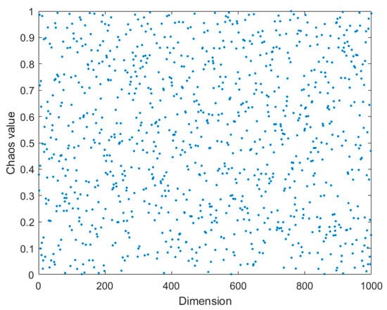
Figure 3.
Chaos value distribution.
- (2)
- Embedding the cooperative search algorithm strategy:
The cooperative search algorithm (CSA) is a heuristic optimization algorithm described by Z. Feng et al. [33]. Inspired by the collaborative behavior of modern enterprise teams, this algorithm is divided into four stages: team building, team communication, reflective learning, and internal competition. In the team communication stage, the global optimal solution A is randomly selected as the chairman, the average global optimal solution B as the board of directors, and the average individual optimal solution C as the supervisory board. Each employee in the team can communicate with the leaders of the chairman, board of directors, and supervisory board to obtain new information. Through information exchange within the population, the scope of knowledge and information dissemination can be expanded, allowing the population to better adapt to changes and quickly obtain the global optimal solution of the optimization problem.
In addition, the rolling behavior in the dung beetle algorithm has a leading role in the dung beetle population, and has a significant impact on the search ability and convergence speed of the algorithm. However, as shown in Formula (13), dung beetles only interact with the worst global beetle in the previous generation in their rolling behavior, lacking information exchange between individuals. In order to make up for this deficiency, inspired by the team communication strategy in cooperative search algorithms, this article introduces a team communication mechanism in dung beetle rolling behavior, replacing the position update strategy in the original dung beetle algorithm with a team communication strategy, guiding individual dung beetles to communicate with other individuals, promoting information dissemination in the population, expanding search space, and improving performance. The global search capability of the dung beetle algorithm has been enhanced. The position update of the improved dung beetle during rolling is shown in Formula (21).
Among them, is the position of the j-th dung beetle in the i-th solution at the t + 1 iteration; is the position of the j-th dung beetle among the i-th group of individuals in t-th iteration; is the position of the j-th beetle in the m-th group of globally optimal beetles from the beginning to the t-th iteration; and indicate coefficients for adjusting and , respectively.
- (3)
- Adaptive t-distribution mutation strategy:
In the later stage of iteration, the dung beetle algorithm will quickly converge to the vicinity of the optimal position, where the solution is close to the optimal solution. However, if the current optimal solution is not the global optimal solution, and the dung beetle population focuses on searching near the current position, it will lead to the problem of not being able to find the true global optimal solution and falling into a local optimal solution. To solve the above problems, introducing a mutation perturbation strategy into the algorithm can enhance the algorithm’s ability to jump out of local optima, allowing the population to traverse the solution space more fully, expand the search range, and finally find the global optimal solution.
In heuristic algorithms, introducing mutation operators can maintain the diversity of the population while avoiding aggregation of the population at local optimal positions. Inspired by Reference [34], this paper introduces adaptive t-distribution mutation perturbation to improve the search strategy of the algorithm. Adaptive t-distribution mutation uses the number of iterations of the algorithm as the degree of freedom parameter of the t-distribution mutation, effectively combining the advantages of the Cauchy distribution and the Gaussian distribution. In the early stage of algorithm iteration, the t-distribution is close to the Cauchy distribution and has good global search ability. As the number of iterations increases, the t-distribution gradually moves towards the Gaussian distribution. At this time, the algorithm has strong local development ability, which can ensure the convergence speed of the algorithm in the later stage of iteration.
In addition, the results obtained by incorporating mutation perturbation have a certain degree of randomness. If mutation perturbation is applied to all beetles, it will increase the complexity of the algorithm. Therefore, this article only applies mutation perturbation to the optimal beetle individual and selects the beetle with a better position to enter the next iteration, effectively increasing the diversity of beetles and improving the search performance of the algorithm. The improved position update is shown in Formula (22).
Among them, is the optimal position of individual i of the dung beetle at the t-th iteration; indicates the position of individual dung beetles that have undergone adaptive t-distribution variation; t(iter) indicates the t-distribution operator with the degree of freedom parameter iter.
3.2. VMD Parameter Optimization Based on CSADBO Algorithm
3.2.1. Parameter Optimization
According to the implementation principle of the VMD algorithm, it is necessary to pre-set the number of modal components K and the penalty factor , and the values of these two parameters play a decisive role in the final decomposition effect [35]. If parameter K is not properly selected, it can easily lead to problems in the decomposition of the signals; if parameter is not selected properly, it will affect the modal components so that they are not in the appropriate bandwidth position. Therefore, if the parameters K and are set improperly, it will affect the extraction and processing of important signal features.
At present, most of the parameter selection methods rely on past experience or reference to numerical values in the literature, but artificially setting parameters often has problems such as randomness and contingency. Therefore, this article selects the CSADBO algorithm to globally adaptively optimize parameters K and of the VMD algorithm, in order to determine the optimal parameter combination [K, ] and achieve the optimal modal decomposition of the vibration signal of rolling bearings.
In addition, when using the CSADBO algorithm to search for the optimal parameter combination, it is necessary to choose a reasonable objective function as the fitness function of the algorithm. And envelope entropy is an indicator used to evaluate the complexity of signals. If the entropy value is low, it indicates that the complexity of the signal is low and the periodicity is obvious; on the contrary, if the entropy value is higher, it indicates that the signal is more complex and there is more noise interference. Envelope entropy can effectively evaluate the sparsity of signals and plays an important role in the fields of mechanical equipment fault diagnosis and operational status monitoring. Therefore, this article chooses envelope entropy to evaluate the decomposition effect of VMD and uses it as the fitness function in the CSADBO algorithm, thereby improving the decomposition effect of VMD through algorithm optimization. The calculation of envelope entropy is shown in Formula (23).
Here, N denotes the number of sampling points; denotes the transformed signal; is the standardized form of .
3.2.2. Feature Selection
After decomposition by the VMD algorithm, multiple IMF components will be obtained, some of which may contribute less to the features or fault information of interest, and if all components are directly analyzed and processed, it will inevitably increase additional computational complexity. The IMF components with smaller envelope entropy values often correspond to vibration components with clearer envelope curves and more prominent fault characteristics [3]. Therefore, this article selects the component with the smallest envelope entropy value as the optimal IMF component, which can better highlight the characteristics of fault signals, help fault diagnosis and monitoring, and reduce unnecessary computational complexity. This is particularly important in scenarios such as large-scale data analysis and real-time monitoring, and can accelerate the speed and response ability of fault diagnosis.
After selecting the optimal IMF component, it is necessary to extract the features of components to construct a feature matrix. Based on the characteristics of the rolling bearing vibration signal, commonly used indicators to evaluate the bearing state include energy, peak value, kurtosis value, skewness value, root mean square, mean value, and arrangement entropy [36]. However, a single-feature indicator cannot comprehensively describe the complexity and fault characteristics of signal components. If a single-feature indicator is selected for diagnosis, it is easy to miss the effective features in the components. However, the comprehensive use of multiple indicators can discover potential fault features from different aspects. Therefore, this article will fuse multi-parameter information to construct a multi-parameter fusion feature matrix. The fused feature indicators include root mean square, variance, peak, energy, skewness, kurtosis, envelope entropy, and permutation entropy. Due to space limitations, some of the selected feature indicators are described as follows:
(1) Energy: Represents the total energy of the vibration signal in the time domain, and bearing failures often result in abnormal changes in the energy of the vibration signal. Energy can be expressed using Formula (24):
(2) Skewness and kurtosis: Skewness and kurtosis can be used to evaluate the distribution characteristics of fault signals. Skewness is used to measure the asymmetry of the vibration signal distribution; kurtosis is used to measure the sharpness of the distribution of vibration signals. Skewness and kurtosis can be expressed using Formulas (25) and (26), respectively.
where denotes the mean of the fault signal; denotes the standard deviation of the signal.
(3) Permutation entropy: Permutation entropy provides a measure of the complexity of time series data and can capture dynamic and nonlinear features of fault signals. The calculation of permutation entropy is shown in Formula (27).
where represents the frequency at which each arrangement appears in the subsequence of the time series signal.
The VMD optimization process based on the CSADBO algorithm is shown in Figure 4:

Figure 4.
VMD optimization process based on CSADBO algorithm.
3.3. Bearing Fault Diagnosis Process Based on Optimized CNN-BiLSTM
In the diagnosis of rolling bearing faults, a CNN can effectively capture the local features and spatial correlations of signals. By using VMD-decomposed features as inputs in a CNN, a CNN can focus more on extracting local features to capture subtle changes in rolling bearing faults; BiLSTM, on the other hand, can model global dependencies at the temporal level. By simultaneously modeling the temporal relationship of rolling bearing vibration signals from both positive and negative directions on a global scale, it can better utilize temporal information; the effective combination of a CNN and BiLSTM can enhance the robustness and generalization ability of a model of rolling bearing faults, enabling it to better adapt to the diagnostic needs of different rolling bearing faults. However, the CNN-BiLSTM model has multiple hyperparameters, such as the number of convolutional kernels, learning rate, and number of hidden layer neurons. The size of parameter values has a significant impact on the performance of the model, and inappropriate values may lead to a decrease in network performance [25]. At present, the above parameters are usually determined based on experience or suggestions from the literature, but the values of the parameters may vary for different application scenarios. To address the above issues, we need an efficient optimization method to adaptively adjust parameter values, in order to enhance performance of the CNN-BiLSTM model in rolling bearing fault diagnosis.
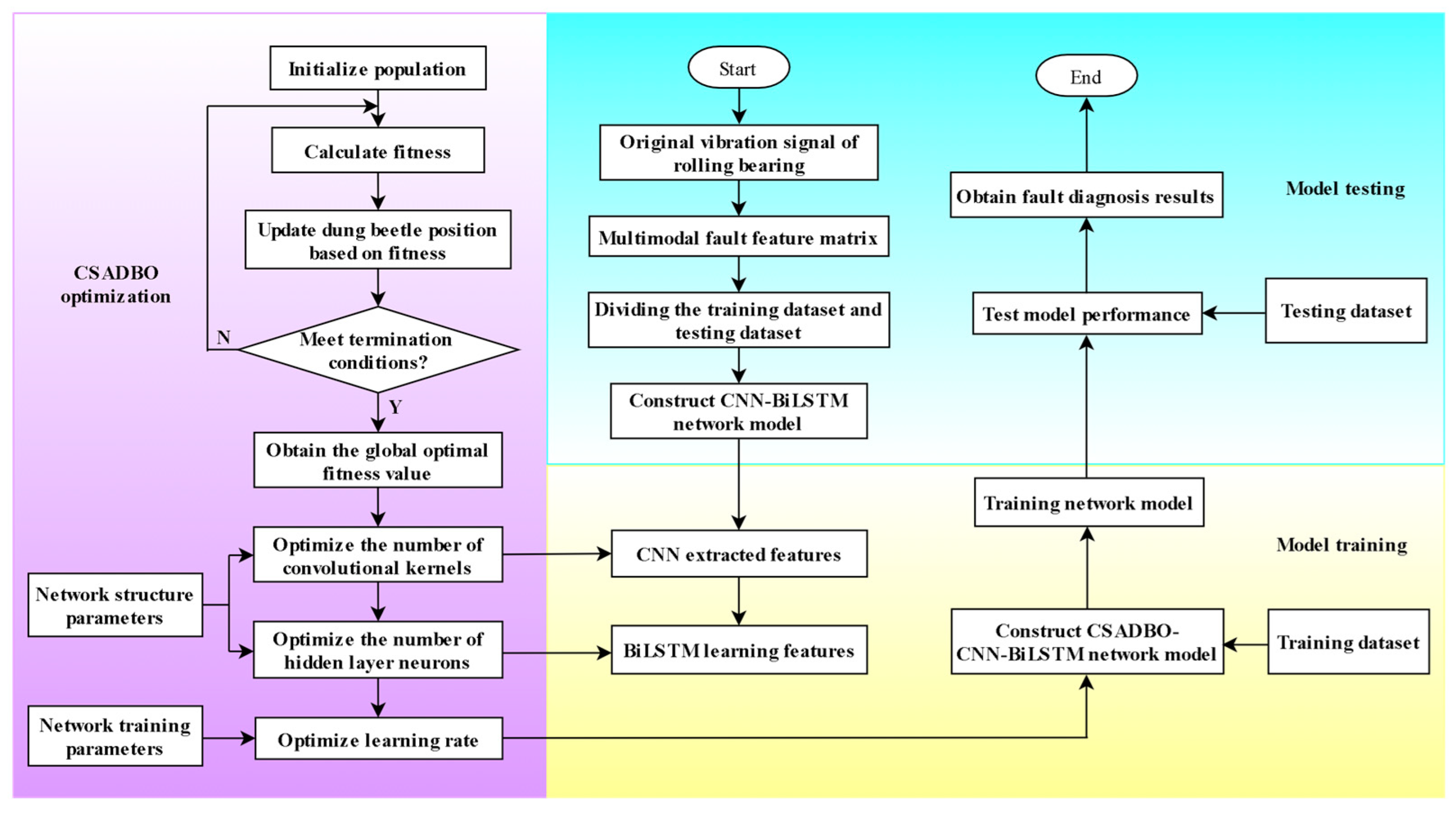
The CSADBO algorithm proposed in Section 3.1 of this article has good optimization performance and convergence speed, and, after various strategy improvements, it solves the problem of easily falling into local optima. Therefore, the CSADBO algorithm is selected to optimize the number of convolutional kernels, learning rate, and number of hidden layer neurons in the CNN-BiLSTM model. Through the optimization process of the CSADBO algorithm, the parameter space can be effectively searched, and a set of model parameter combinations with the best performance in rolling bearing fault diagnosis can be found. The optimized parameters are applied to the CNN-BiLSTM model to improve the performance and accuracy of the model in fault diagnosis tasks. Through this approach, it is possible to avoid manually selecting parameters and consuming a lot of manpower and time, and to fully utilize the optimization ability of the algorithm to achieve better model performance. The bearing fault diagnosis process based on optimized CNN-BiLSTM is shown in Figure 5.
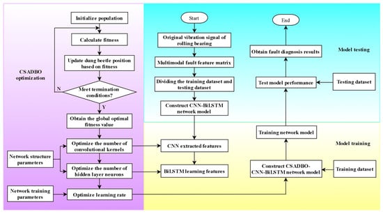
Figure 5.
Fault diagnosis process for bearings based on optimized CNN-BiLSTM.
4. Rolling Bearing Fault Diagnosis Model Based on CSADBO-VMD-CNN-BiLSTM
By performing modal decomposition on the fault signal of rolling bearings using the VMD algorithm, K modal components are extracted to obtain multi-scale signal feature representations, which helps to more comprehensively describe the fault state of rolling bearings. Then, key features are extracted based on the optimal modal components corresponding to each type of fault to construct a feature matrix. Finally, the feature matrix is input into the fault diagnosis model to complete the classification of fault signals. The overall technical roadmap is shown in Figure 6.
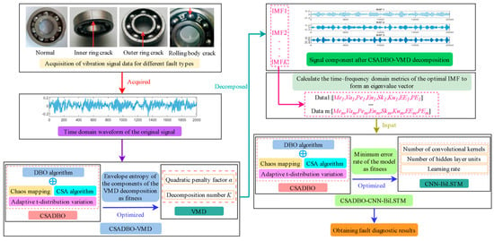
Figure 6.
Rolling bearing fault diagnosis model based on CSADBO-VMD-CNN-BiLSTM.
The specific implementation steps of a rolling bearing fault diagnosis model based on CSADBO-VMD-CNN-BiLSTM are as follows:
Step 1: Collect signals: Use sensors to collect the vibration signals of rolling bearings under four different states: normal, inner ring fault, outer ring fault, and rolling element fault.
Step 2: Raw signal processing: Using the CSADBO algorithm to search for the optimal VMD parameter combination of bearings in different states [K, ]. Then, based on the optimized results, the VMD algorithm is initialized with parameters, and the fitness function is the minimum envelope entropy of each modal component of the vibration signal.
Step 3: Signal decomposition: Use the optimized VMD algorithm to decompose the signal samples and obtain K IMF components .
Step 4: Signal extraction: Select the IMF component with the smallest envelope entropy value as the optimal component, and then calculate the key time–frequency characteristic values in the optimal component to form a feature matrix .
Step 5: Model training: Divide the feature matrix into training and testing sets in an 8:2 ratio, and use the proposed CSADBO algorithm to optimize the number of convolutional kernels, learning rate, and number of hidden layer neurons in the CNN-BiLSTM model. At the same time, use the optimal parameters to train the CNN-BiLSTM model.
Step 6: Testing: Input the test set samples into the trained CNN-BiLSTM model and output fault classification results to verify the effectiveness of the model.
5. Simulation Testing Experiments and Experimental Research Based on Public Datasets
5.1. CSADBO Algorithm Testing Experiment
The algorithm simulation test experiment in this article is based on the Windows 10 64 bit operating system, with an Intel i5-12400F 2.50 GHz processor, 16 GB of running memory, and the MATLAB R2023b programming environment. The manufacturer of the Windows 10 operating system is Microsoft Corporation, headquartered in Redmond, Washington, USA.
To test the performance of the improved algorithm in this paper, the CSADBO algorithm was compared with the DBO algorithm, peafowl optimization algorithm (POA) [37], grey wolf optimizer (GWO) [38], golden jackal optimization, GJO) [39], the artificial protozoa optimizer (APO) [40], and black kite algorithm (BKA) [41], which are used to perform optimality finding comparison experiments on CEC2005 test functions. CEC2005 contains 25 benchmark test functions. Due to limited space, but in order to maintain generality, this article randomly selects four types of unimodal and bimodal test functions. The test functions are shown in Table 1, where F1, F2, F4, and F6 are unimodal test functions with a single optimal value; that is, the local optimal value is equivalent to the global optimal value, which can be used to test the convergence speed of the algorithm during the iteration process; F7, F9, F12, and F13 are multimodal test functions with multiple local extremum points, which can be used to test whether the algorithm can avoid falling into local optima.

Table 1.
Benchmarking test function.
In the simulation experiment, the population size of the algorithm was set to 30 and the upper limit of iterations was 1000. In order to reduce the impact of the randomness of the heuristic optimization algorithm and improve the persuasiveness of the test results, each algorithm that needed to be tested was run 30 times separately on eight standard test functions. In order to visually compare the convergence accuracy and speed of eight algorithms, the mean of the 30 simulation results was calculated and the fitness iteration convergence curves of different algorithms were plotted, as shown in Figure 7.
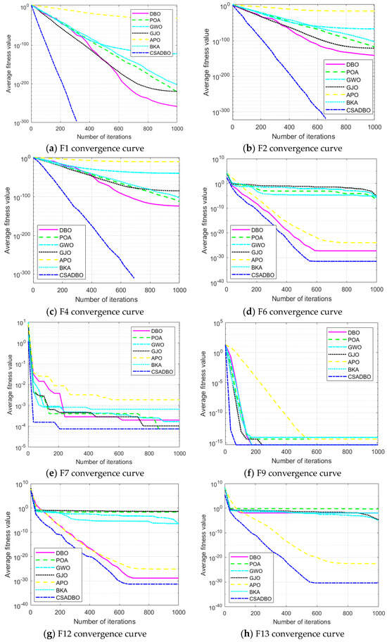
Figure 7.
Comparison of function convergence curves for different algorithms.
Figure 7a–d show the performance of the algorithm during testing on a unimodal function. From Figure 7a–d, it can be seen that, compared with other algorithms, the CSADBO algorithm proposed in this paper has a faster convergence speed in the initial period, indicating that the introduced Cubic chaotic mapping strategy has increased the diversity of initial solutions in the population, improved the global exploration performance of the algorithm, and enabled the algorithm to not only converge quickly in the early stages of iteration, but also continue to optimize as the number of iterations increases until the global optimal solution is found, without any search stagnation. Figure 7e–h show the performance of the algorithm during testing on multimodal functions, where there are multiple extreme points. From Figure 7e–h, it can be seen that the convergence curve has multiple inflection points, indicating that the cooperative search strategy and adaptive t-distribution strategy embedded in the original DBO algorithm in this paper can make the algorithm jump out of the local optimum well, and the convergence accuracy has been greatly improved. It can be seen that the improvement strategy proposed in this paper is effective, and, compared with other algorithms, CSADBO shows better performance in terms of its fast convergence speed and optimal search accuracy.
5.2. CSADBO-VMD-CNN-BiLSTM Fault Diagnosis Model Testing Experiment
5.2.1. Source of Experimental Data
The experimental data used in this paper are from the Rolling Bearing Data Center of Case Western Reserve University (CWRU) (data acquisition address: https://engineering.case.edu/bearingdatacenter/download-data-file), accessed on 15 May 2024. These data are used to verify the effectiveness of the fault diagnosis model proposed in this article; the fault diagnosis experimental platform is shown in Figure 8. The experimental platform consists of asynchronous motors, torque sensors, and power testers. The tested bearing model is SKF6205, and the acceleration sensor is placed above the base of the bearing to be diagnosed at the motor drive end. The collected fault types of the rolling bearings are divided into rolling element, inner ring, and outer ring faults, each of which includes four fault sizes: 0.007, 0.014, 0.021, and 0.028 inches. This article randomly selected samples of three types of fault sizes for experimental testing. The specific experimental data are as follows: bearing normal state data collected at a sampling frequency of 12 kHz, 0 load condition (motor speed of 1797 r/min), and fault state data with fault sizes of 0.007, 0.014, and 0.021 inches. Therefore, there are a total of 10 states, namely 10 different categories. Taking the bearing signal with a fault size of 0.007 inches as an example, the waveforms corresponding to four different categories of states are shown in Figure 9.
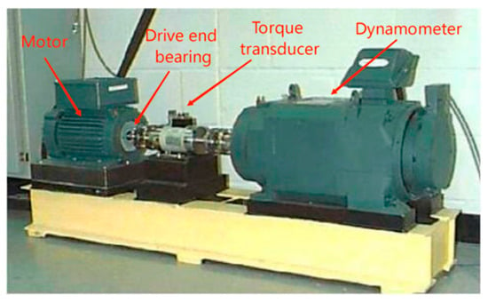
Figure 8.
Experimental setup diagram.
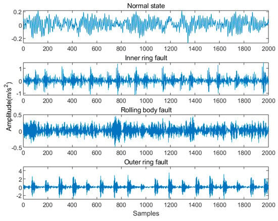
Figure 9.
Vibration signal waveforms of four different states of bearings.
In this experiment, in order to ensure the better capture of periodic features and fault data in bearing vibration signals, 2048 data points (approximately five cycles of data points) were selected for each sample, and sliding windows were used to sample the data for each state. There were 120 samples selected for each state, totaling 1200 samples. Then, 80% of these samples were selected as training samples, and the remaining 20% were used as testing samples. The detailed bearing fault sample data are shown in Table 2.

Table 2.
Sample data of bearing fault.
5.2.2. Analysis of Experimental Results
- (1)
- VMD parameter optimization test
In accordance with the VMD parameter optimization method described in Section 3.2 above, this section conducts simulation experiments to test the feasibility of the proposed method. Firstly, the CSADBO algorithm described in this article is used to optimize the parameters of the VMD algorithm, in order to find the optimal parameter combination [K, ]. Taking the bearing inner ring fault signal with a fault size of 0.007 inches as an example, the minimum envelope entropy of the modal component of the inner ring fault signal is used as fitness function. The search range for the number of modes K is set to [2, 10], the search range for the penalty factor is set to [50, 2500], the initial size of the dung beetle population is set to 10, and the maximum number of iterations is set to 20.
Due to the randomness of heuristic optimization algorithms, there may be some differences in the results of each iteration. This is because the population is reinitialized during each iteration, so the optimization results may not be completely consistent. Therefore, in order to maintain generality, this article takes the average of five experiments as the result. The experimental results are shown in Figure 10. From Figure 10a, it can be seen that the penalty factor has converged to the optimal value in the 8th iteration, and the final convergence value is 1583; Figure 10b shows the iteration curve of the number of modes, which has converged to the optimal value in the third iteration. The optimal number of mode decompositions is 5; Figure 10c shows the iteration curve of envelope entropy, which converges at the 5th iteration with a minimum envelope entropy of 7.3411.
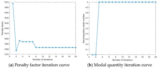
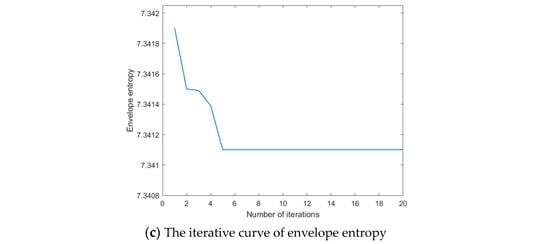
Figure 10.
CSADBO-VMD iteration curve.
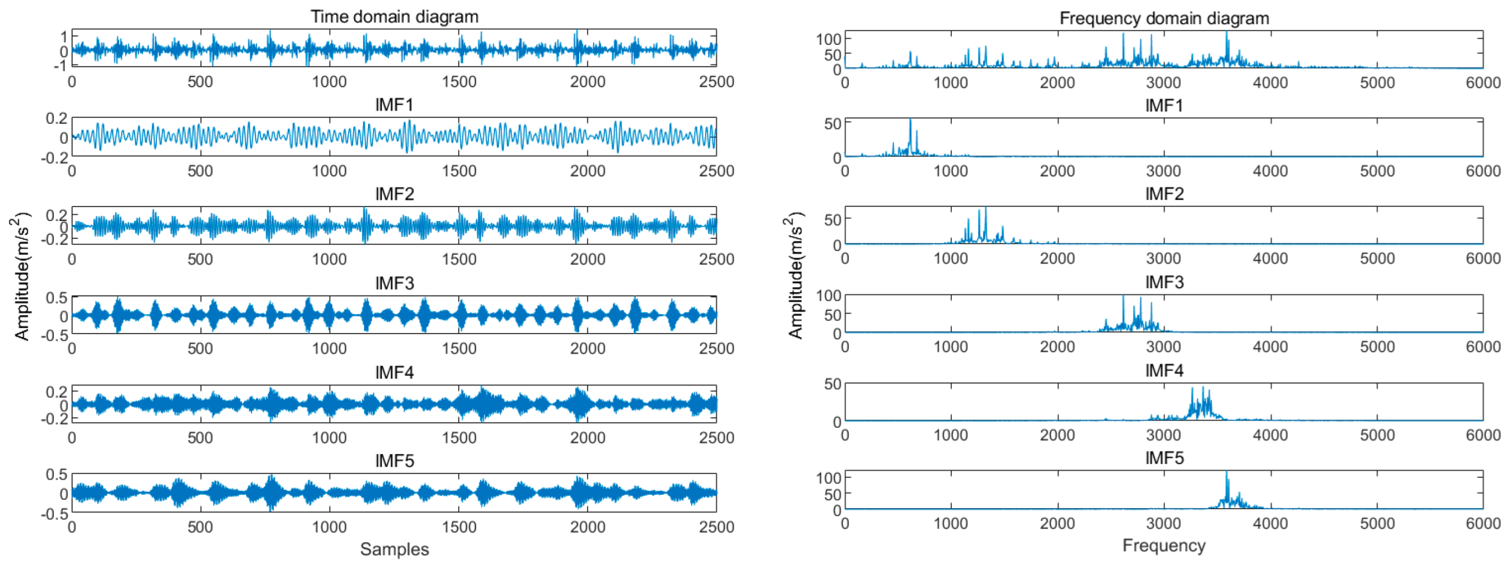
Therefore, the optimal parameter combination for the VMD algorithm can be obtained as [K, ] = [5, 1583], and then the optimal parameters are substituted into the VMD algorithm to perform modal decomposition on the inner ring fault signal. The decomposed result is shown in Figure 11. It can be clearly seen from Figure 11 that there is no modal aliasing phenomenon between the spectra of each component, which can be well used to describe the fault characteristics. In order to highlight the decomposition effect, a comparison was made with the decomposition effect of the artificially set parameter combination of [K, ] = [4, 2000] in Reference [42]. The decomposition results of the parameter combination of [4, 2000] are shown in Figure 12. By comparison, it can be seen that the optimized parameters in this article have an additional IMF4 component in the decomposition results. Based on the amplitude of the frequency domain diagram of the inner circle fault signal, the IMF4 component can be used to characterize the characteristics of the fault, while the IMF4 component is missing in Figure 12. Therefore, there is uncertainty in manually setting parameters, which can easily ignore the characteristics of the signal. This indicates that the optimized VMD algorithm in this article can effectively extract the features of fault signals.
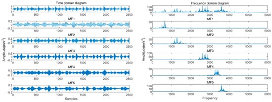
Figure 11.
Time–frequency domain diagram of IMF components after CSADBO-VMD.
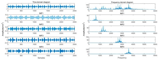
Figure 12.
Time–frequency domain diagram of IMF components after VMD ([K, ] = [4, 2000]).
- (2)
- Fault diagnosis accuracy test
This section conducts performance testing on the fault diagnosis model proposed in the paper, using the CSADBO algorithm to optimize the number of convolutional kernels, number of hidden layer neurons, and the learning rate in the neural network model. The experimental environment is based on the Windows 10 64 bit operating system, with a processor type of Intel i5-12400F 2.50 GHz, a GPU type of NVIDIA GeForce RTX4060 Ti, a running memory of 16 GB, and a programming environment of MATLAB R2023b.
In order to better search for the optimal combination of hyperparameters in the network model, we need to set the range of hyperparameter values, where the range of the number of convolutional kernels is [5, 50], the range of the number of hidden layer neurons is [10, 200], and the range of the learning rate is [0.001, 0.2]. In the CSADBO algorithm, the population size of the beetle is set to 10 and the number of iterations is set to 10. The corresponding hyperparameters obtained by optimizing the CNN-BiLSTM model using the CSADBO algorithm are shown in Table 3.

Table 3.
Parameters of CSADBO-VMD-CNN-BiLSTM model.
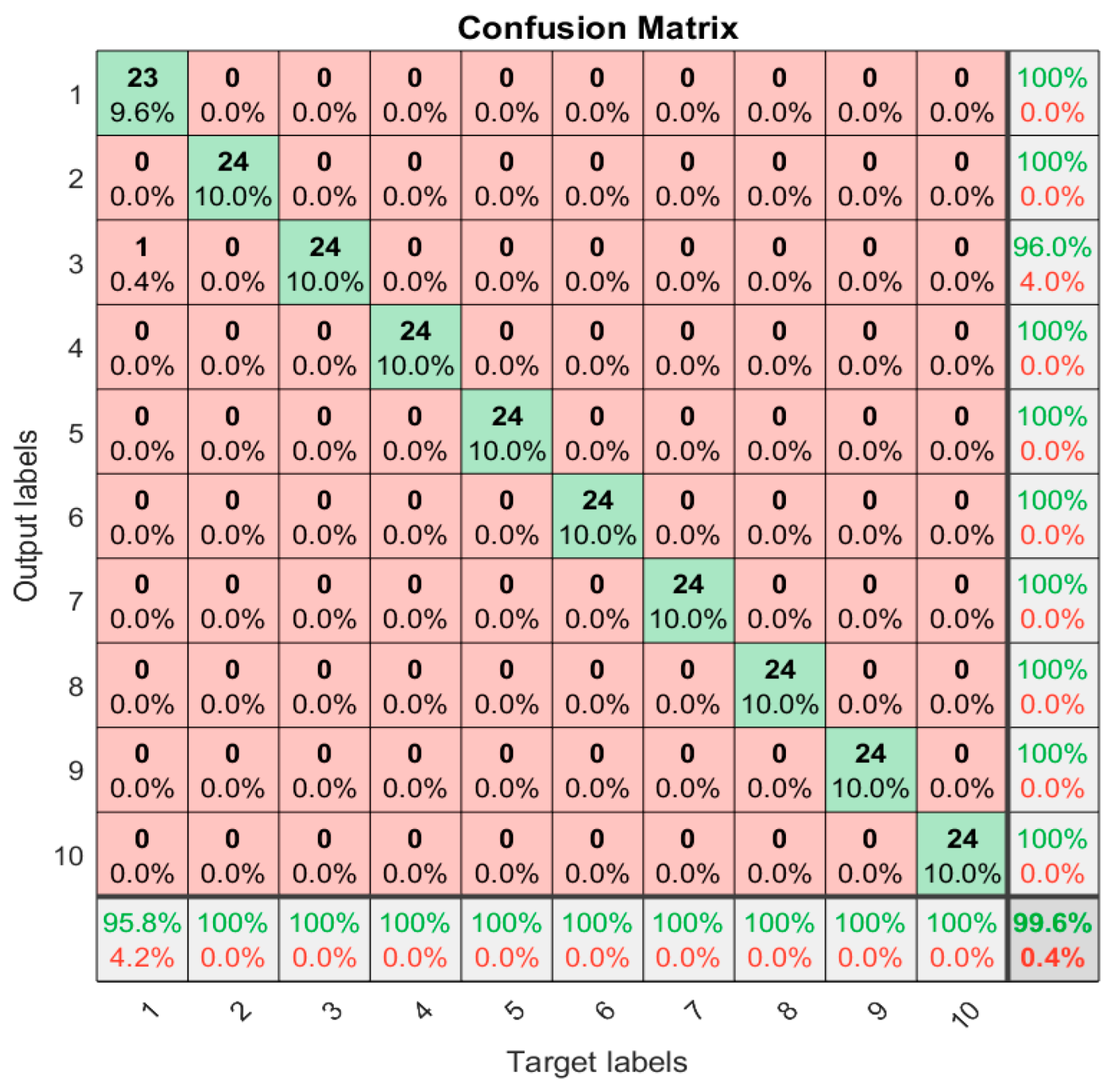
From Table 3, it can be seen that the optimal network parameters optimized by the CSADBO algorithm are as follows: the number of convolutional kernels = [12, 19], the number of hidden layer neurons = [80, 55], and the learning rate is 0.0238. After searching for the optimal parameters, the parameters are substituted back into the model for retraining, and then the fault diagnosis performance of the model is evaluated using the test set. Through experimental testing of the model, the optimization model described in this article shows fault classification results for ten states in Figure 13, and Figure 14 shows the confusion matrix of the fault diagnosis results. From Figure 13 and Figure 14, it can be seen that, out of 240 test samples, 239 were correctly classified, and only one normal sample was misclassified as an outer ring fault. The model achieved a recognition accuracy of 99.6% in the test set. From this, it can be seen that the CSADBO-VMD-CNN-BiLSTM model described in this article has a high recognition accuracy for fault classification of new and unprecedented data, good generalization ability, and excellent performance in rolling bearing fault diagnosis.
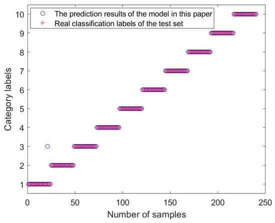
Figure 13.
Results of CSADBO-VMD-CNN-BiLSTM model testing.
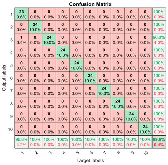
Figure 14.
Confusion matrix.
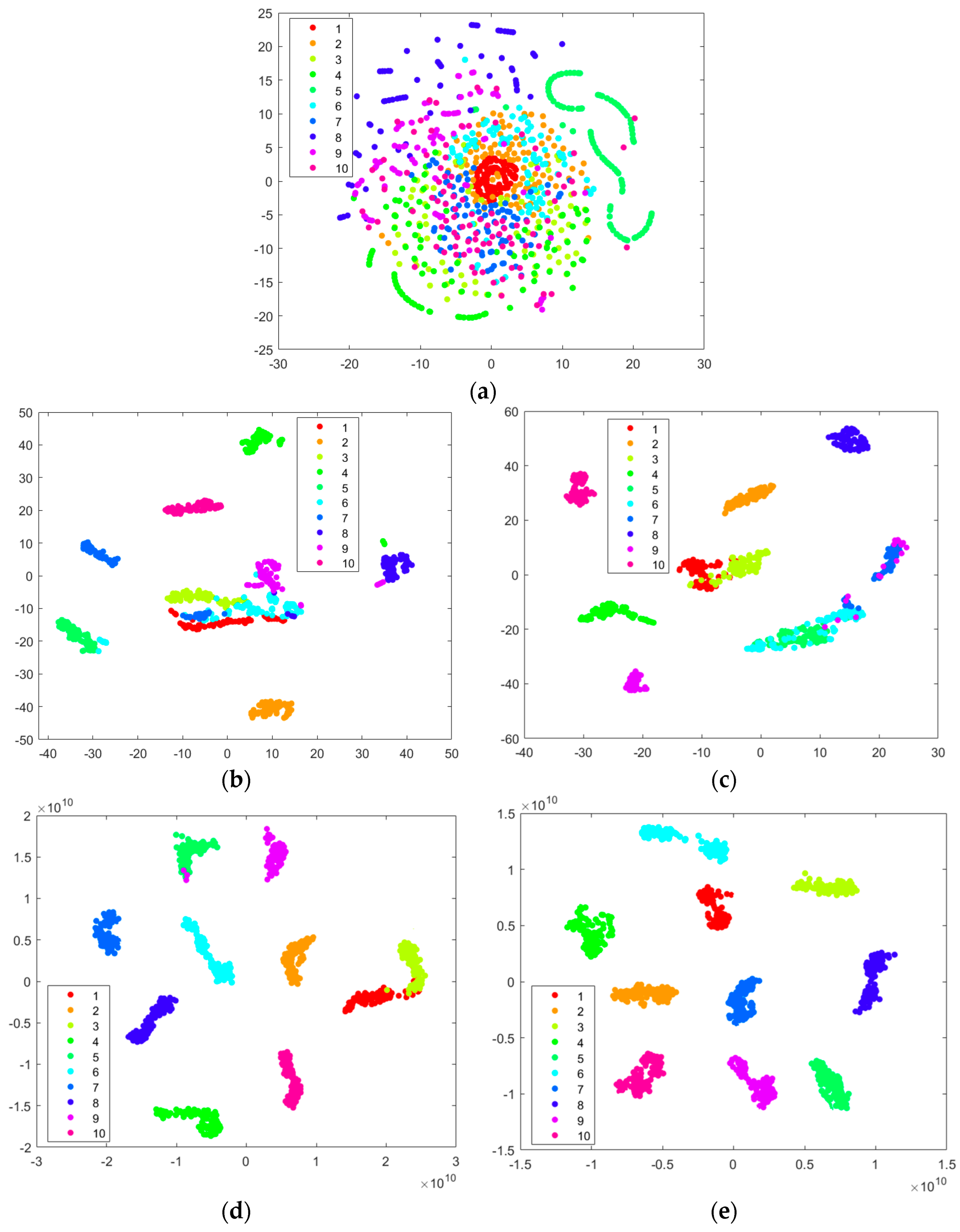
In order to more intuitively test the effectiveness of the model proposed in this article in rolling bearing fault diagnosis, the t-SNE method was used to visualize the distribution of bearing fault sample data, as shown in Figure 15. The horizontal and vertical coordinates represent the first and second coordinates after the t-SNE dimensionality reduction, respectively. The more dispersed the distribution of each type of fault sample in the figure, the better the classification effect. By comparing the (a–e) figures in Figure 15, it can be seen that the distribution of the original fault samples in Figure 15a is relatively chaotic, and the aliasing phenomenon is severe, which can lead to unsatisfactory classification results; Figure 15b represents the sample distribution after feature extraction by the VMD algorithm, which can straightforwardly show the distribution of samples in different categories. However, randomly setting VMD parameters can lead to the poor decomposition performance of the algorithm, resulting in samples in categories 1, 3, 6, and 9 being in an aliased state; Figure 15c shows the sample distribution of VMD optimized by the CSADBO algorithm. The fault feature distribution has a more significant classification effect compared to Figure 15b, effectively reducing the phenomenon of aliasing; Figure 15d shows the sample distribution after being processed by the CNN-BiLSTM model based on Figure 15c, but due to the suboptimal model parameters, there is a phenomenon of incomplete separation between individual samples; Figure 15e shows the results of the CNN-BiLSTM model optimized by the CSADBO algorithm. It can be clearly seen that at this time, samples of the same fault type are basically clustered together, and there is no aliasing phenomenon in the distribution between different fault categories. Therefore, the ten fault types can be distinguished well. Therefore, the above comparison can indirectly show that the model proposed in this paper is effective and can be effectively applied in the field of bearing fault diagnosis.
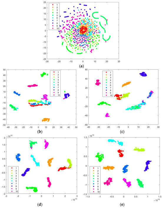
Figure 15.
Visualization results of t-SNE: (a) the distribution of the original sample; (b) the distribution of samples after VMD; (c) the distribution of samples after CSADBO-VMD; (d) the distribution of samples after recognition by the CSADBO-VMD-CNN-BiLSTM model (where the hyperparameters of CNN-BiLSTM are not optimized); (e) the distribution of samples after model recognition in this article (optimizing hyperparameters for VMD and CNN-BiLSTM).
- (3)
- Comparative testing of models under different parameters
In order to test that the CSADBO algorithm was used to search for the optimal parameter combination in this article, we conducted a set of comparative experiments by controlling variables. The initial parameters used were as follows: the number of convolutional kernels = [8, 16], the number of hidden layer neurons = [10, 10], and the learning rate value was 0.1. Meanwhile, during the training of the model, the data order is randomized and shuffled at each iteration to improve the generalization of the model and reduce the risk of overfitting. However, this can also lead to slight differences in the experimental results. Therefore, in order to maintain generality, CNN-BiLSTM models with different parameters were subjected to five repeated experiments and an average value was taken. The experimental results are shown in Table 4 and Figure 16, where 0, 1, 2, 3, and 4, respectively, represent the initial setting of the parameters, the number of convolutional kernels with optimal parameters, the number of hidden layer neurons with optimal parameters, the learning rate with optimal parameters, and all parameters with optimal parameters. From Table 4 and Figure 16, it can be seen that due to large randomness and the randomness of parameter values set by experience in the network model, the selection of parameters is not scientific enough. Therefore, the average accuracy of bearing fault diagnosis is 93.0%. When using the control variable method to set the three parameters of the CNN-BiLSTM model to the best individual values, compared with the CNN-BiLSTM model set of initial parameters, the diagnostic accuracy obtained increased by 1.6%, 5.2%, and 3.3%, respectively. When the parameters of the model are all optimal, the average accuracy obtained is 99.6%. Compared with the initial parameters and the model with a single optimal parameter, the accuracy increased by 6.6%, 5.0%, 1.4%, and 3.3%, respectively. Therefore, it can be fully proved that the CSADBO-VMD-CNN-BiLSTM bearing fault diagnosis model described in this paper has a high diagnostic accuracy, verifying the effectiveness of the model.

Table 4.
Fault diagnosis accuracy of model under different parameters.
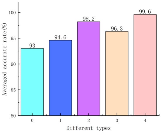
Figure 16.
Fault diagnosis accuracy of the model under different parameters.
- (4)
- Comparative testing of different models
In order to further highlight the diagnostic advantages of the model described in this article, we selected the CNN-BiLSTM, VMD-CNN-BiLSTM, and GWO to optimize both the VMD and CNN-BiLSTM models (GWO-VMD-CNN-BiLSTM), and the DBO to optimize both the VMD and CNN-BiLSTM models (DBO-VMD-CNN-BiLSTM) for simulation experiments on rolling bearing fault diagnosis, and compared them with the model described in this paper. And in order to maintain generality, five repeated experiments were conducted on the models compared above, and the experimental results are shown in Table 5 and Figure 17.

Table 5.
Accuracy of fault diagnosis for different models.
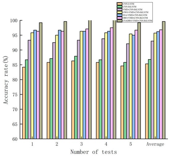
Figure 17.
Fault diagnosis accuracy of different models.
From Table 5, it can be seen that the accuracy of the CNN-LSTM model with the introduction of BiLSTM is improved by 1.5% compared to the traditional CNN-LSTM; the accuracy of fault classification using the VMD algorithm after signal preprocessing has been significantly improved. Compared to CNN-BiLSTM, the accuracy of the VMD-CNN-BiLSTM model has increased by 6.2%. However, due to the current suboptimal parameters of both VMD and CNN-BiLSTM models, there is still room for improvement in the accuracy of the model. When using the GWO, sparrow search algorithm (SSA) [43], and DBO heuristic algorithms to simultaneously optimize hyperparameters of VMD and CNN-BiLSTM, each model showed excellent performance. GWO-VMD-CNN-BiLSTM, SSA-VMD-CNN-BiLSTM, and DBO-VMD-CNN-BiLSTM improved by 2.7%, 3.2%, and 3.8% compared to VMD-CNN-BiLSTM, respectively. It can be seen that the model optimized by parameters has higher diagnostic accuracy, and compared to the VMD-CNN-BiLSTM model optimized by the GWO and SSA algorithms, the model optimized by the DBO algorithm has better diagnostic accuracy. Better results were obtained after parameter optimization using the CSADBO algorithm described in this paper, and the diagnostic accuracy was improved by 2.8% compared to the model optimized by the DBO algorithm, with an average accuracy of 99.6%. Figure 17 shows the difference in diagnostic accuracy among different models, where the horizontal axis represents the results of five independent experiments and the average experimental results. When the CSADBO algorithm is used to optimize the parameters of VMD and CNN-BiLSTM simultaneously, the accuracy of fault diagnosis is the highest, fully proving the feasibility and superiority of the CSADBO-VMD-CNN-BiLSTM bearing fault diagnosis method described in this paper.
6. Conclusions
Rolling bearing fault diagnosis plays an important role in improving the reliability and stability of mechanical equipment operation. However, traditional fault diagnosis methods have problems such as low diagnostic accuracy and poor generalization performance. Therefore, in order to achieve a better diagnosis of bearing faults, this paper proposes a rolling bearing fault diagnosis model based on an improved DBO algorithm optimized VMD-CNN-BiLSTM. The effectiveness of the described model is demonstrated through simulation tests on the CWRU dataset and comparative experiments with other models. The research is summarized below:
- (1)
- The DBO algorithm was optimized by introducing chaotic mapping, cooperative search, and an adaptive t-distribution mutation strategy. An improved DBO algorithm (CSADBO) was described, which overcomes the problem of imbalanced global exploration and the local development capabilities of the original DBO algorithm. Through simulation experiments, it has been proved that the CSADBO algorithm has a faster convergence speed and performs well in jumping out of local optima.
- (2)
- A parameter optimization method based on the CSADBO algorithm for VMD and CNN-BiLSTM was proposed. The CSADBO algorithm was used to adaptively search for optimal parameters, avoiding randomness and uncertainty caused by manually setting parameters. Multiple experiments were conducted, and specific parameter combinations were provided in the paper.
- (3)
- The model described in this paper was experimentally validated on the CWRU dataset, and it was demonstrated through experimental testing that the model can effectively extract fault signal features and has high diagnostic accuracy. Through five repeated experiments, the average accuracy reached 99.6%, and comparative experiments were conducted with seven other models to further test the effectiveness of the proposed model.
In summary, the fault diagnosis model proposed in this article has excellent diagnostic accuracy and good generalization performance in the diagnosis of rolling bearings. However, in order to enhance the wide applicability of the model, future research will focus on expanding the adaptability of the model to achieve fault diagnosis for other devices.
Author Contributions
Conceptualization, W.S. and X.Z.; methodology, W.S.; software, W.S. and Y.W.; validation, W.S. and X.Y.; formal analysis, J.Z. and D.Z.; investigation, X.Z. and W.S.; resources, X.Z. and Y.W.; data curation, W.S. and X.Y.; writing—original draft preparation, W.S. and J.Z.; writing—review and editing, J.Z. and D.Z.; visualization, X.Z. and W.S.; supervision, D.Z. and J.Z.; project administration, X.Z. and Y.W.; funding acquisition, X.Z. and X.Y. All authors have read and agreed to the published version of the manuscript.
Funding
This research was funded by the Special Fund for Basic Research Business Expenses of Central Universities, grant number 2020ZDPY0223.
Data Availability Statement
The data presented in this study are openly available in the Case Western Reserve University Bearing Data Center at https://engineering.case.edu/bearingdatacenter/download-data-file, accessed on 15 May 2024.
Acknowledgments
All the authors of this paper would like to sincerely thank Case Western Reserve University for publishing the experimental dataset of rolling bearing failure on the internet. In addition, this study was supported by the Special Fund for Basic Research Business Expenses of Central Universities, with the approval number 2020ZDPY0223.
Conflicts of Interest
The authors declare that they have no conflicts of interest to report regarding the present study.
References
- Yu, Y.; Gu, X.; Ma, W.; Guo, L.; Gao, H.; Zhang, G. A New Method for Quantitative Estimation of Rolling Bearings under Variable Working Conditions. IEEE/ASME Trans. Mechatron. 2024, 29, 41–51. [Google Scholar] [CrossRef]
- Zhao, H.; Liu, H.; Jin, Y.; Dang, X.; Deng, W. Feature extraction for data-driven remaining useful life prediction of rolling bearings. IEEE Trans. Instrum. Meas. 2021, 70, 3511910. [Google Scholar] [CrossRef]
- Tan, C.; Yang, L.; Chen, H.; Xin, L. Fault diagnosis method for rolling bearing based on VMD and improved SVM optimized by METLBO. J. Mech. Sci. Technol. 2022, 36, 4979–4991. [Google Scholar] [CrossRef]
- Song, X.; Wang, H.; Liu, Y.; Wang, Z.; Cui, Y. A fault diagnosis method of rolling element bearing based on improved PSO and BP neural network. J. Intell. Fuzzy Syst. 2022, 43, 5965–5971. [Google Scholar] [CrossRef]
- Meng, D.; Wang, H.; Yang, S.; Lv, Z.; Hu, Z.; Wang, Z. Fault analysis of wind power rolling bearing based on EMD feature extraction. CMES-Comput. Model. Eng. Sci. 2022, 130, 543–558. [Google Scholar] [CrossRef]
- Zhang, L.; Wang, Z.; Quan, L. Research on weak fault extraction method for alleviating the mode mixing of LMD. Entropy 2018, 20, 387. [Google Scholar] [CrossRef]
- Dragomiretskiy, K.; Zosso, D. Variational mode decomposition. IEEE Trans. Signal Process. 2014, 62, 531–544. [Google Scholar] [CrossRef]
- Huang, D.; Li, Y.; Guan, S.; Zhang, X.; Tang, M. A novel collaborative diagnosis approach of incipient faults based on VMD and SCN for rolling bearing. Optim. Control Appl. Methods 2023, 44, 1617–1631. [Google Scholar] [CrossRef]
- Fu, L.; Ma, Z.; Wu, D.; Liu, J.; Xu, F.; Zhong, Q.; Zhu, T. BearingCog: A Bearing Fault Diagnosis Method under Variable Operational Conditions. Appl. Sci. 2022, 12, 5240. [Google Scholar] [CrossRef]
- Liu, C.; Tan, J. An enhanced variational mode decomposition based on correntropy and a periodicity-assisted log-cycligram for bearing fault diagnosis. Meas. Sci. Technol. 2022, 33, 065108. [Google Scholar] [CrossRef]
- Chen, S.; Kang, M.; Liang, C.; Xu, T.; Yu, J. Electricity Load Forecasting Based on DBO Optimized VMD Decomposition and Feature Screening. In Proceedings of the 2023 3rd International Conference on Intelligent Power and Systems (ICIPS), Shenzhen, China, 20–22 October 2023; pp. 499–505. [Google Scholar] [CrossRef]
- Tan, S.; Wang, A.; Shi, H.; Guo, L. Rolling bearing incipient fault detection via optimized VMD using mode mutual information. Int. J. Control Autom. Syst. 2022, 20, 1305–1315. [Google Scholar] [CrossRef]
- Wang, M.; Wang, W.; Zeng, J.; Zhang, Y. An integrated method based on sparrow search algorithm improved variational mode decomposition and support vector machine for fault diagnosis of rolling bearing. J. Vib. Eng. Technol. 2022, 10, 2893–2904. [Google Scholar] [CrossRef]
- Wang, Z.; Wang, S.; Cheng, Y. Fault Feature Extraction of Parallel-Axis Gearbox Based on IDBO-VMD and t-SNE. Appl. Sci. 2023, 14, 289. [Google Scholar] [CrossRef]
- Dou, D.; Jiang, J.; Wang, Y.; Zhang, Y. A rule-based classifier ensemble for fault diagnosis of rotating machinery. J. Mech. Sci. Technol. 2018, 32, 2509–2515. [Google Scholar] [CrossRef]
- Liu, X.; Sun, W.; Li, H.; Hussain, Z.; Liu, A. The method of rolling bearing fault diagnosis based on multi-domain supervised learning of convolution neural network. Energies 2022, 15, 4614. [Google Scholar] [CrossRef]
- Liu, B.; Cai, J.; Peng, Z. Rolling Bearing Fault Diagnosis Method Based on VMD-IMDE-PNN. Noise Vib. Control 2022, 42, 96–101+133. [Google Scholar]
- Eren, L.; Ince, T.; Kiranyaz, S. A generic intelligent bearing fault diagnosis system using compact adaptive 1D CNN classifier. J. Signal Process. Syst. 2019, 91, 179–189. [Google Scholar] [CrossRef]
- Pan, H.; He, X.; Tang, S.; Meng, F. An improved bearing fault diagnosis method using one-dimensional CNN and LSTM. Stroj. Vestn.-J. Mech. Eng. 2018, 64, 443–452. [Google Scholar]
- Zhao, D.; Li, J.; Cheng, W.; Wen, W. Bearing multi-fault diagnosis with iterative generalized demodulation guided by enhanced rotational frequency matching under time-varying speed conditions. ISA Trans. 2023, 133, 518–528. [Google Scholar] [CrossRef]
- Zhao, D.; Cui, L.; Liu, D. Bearing Weak Fault Feature Extraction Under Time-Varying Speed Conditions Based on Frequency Matching Demodulation Transform. IEEE/ASME Trans. Mechatron. 2023, 28, 1627–1637. [Google Scholar] [CrossRef]
- Cui, L.; Li, W.; Wang, X.; Zhao, D.; Wang, H. Comprehensive remaining useful life prediction for rolling element bearings based on time-varying particle filtering. IEEE Trans. Instrum. Meas. 2022, 71, 3510010. [Google Scholar] [CrossRef]
- Zhao, D.; Wang, H.; Cui, L. Frequency-chirprate synchrosqueezing-based scaling chirplet transform for wind turbine nonstationary fault feature time–frequency representation. Mech. Syst. Signal Process. 2024, 209, 111112. [Google Scholar] [CrossRef]
- You, D.; Chen, L.; Liu, F.; Zhang, Y.; Shang, W.; Hu, Y.; Liu, W. Intelligent fault diagnosis of bearing based on convolutional neural network and bidirectional long short-term memory. Shock. Vib. 2021, 2021, 7346352. [Google Scholar] [CrossRef]
- Tian, H.; Fan, H.; Feng, M.; Cao, R.; Li, D. Fault diagnosis of rolling bearing based on hpso algorithm optimized cnn-lstm neural network. Sensors 2023, 23, 6508. [Google Scholar] [CrossRef]
- Song, B.; Liu, Y.; Fang, J.; Liu, W.; Zhong, M.; Liu, X. An optimized CNN-BiLSTM network for bearing fault diagnosis under multiple working conditions with limited training samples. Neurocomputing 2024, 574, 127284. [Google Scholar] [CrossRef]
- Zhang, C.; Wang, C.S.; Zhang, D.; Li, L.; Yang, S. Improved Probabilistic Neural Network Based Fault Diagnosis of Control Valve. In Proceedings of the 2023 CAA Symposium on Fault Detection, Supervision and Safety for Technical Processes (SAFEPROCESS), Yibin, China, 22–24 September 2023; IEEE: Piscataway, NJ, USA, 2023; pp. 1–6. [Google Scholar]
- Chang, C.; Liang, C.; Hu, P. Iterative random training sampling convolutional neural network for hyperspectral image classification. IEEE Trans. Geosci. Remote Sens. 2023, 61, 5513526. [Google Scholar] [CrossRef]
- Wang, K.; Ma, C.; Qiao, Y.; Lu, X.; Hao, W.; Dong, S. A hybrid deep learning model with 1DCNN-LSTM-Attention networks for short-term traffic flow prediction. Phys. A Stat. Mech. Its Appl. 2021, 583, 126293. [Google Scholar] [CrossRef]
- Guo, K.; Wang, N.; Liu, D.; Peng, X. Uncertainty-aware LSTM based dynamic flight fault detection for UAV actuator. IEEE Trans. Instrum. Meas. 2022, 72, 3502113. [Google Scholar] [CrossRef]
- Xue, J.; Shen, B. Dung beetle optimizer: A new meta-heuristic algorithm for global optimization. J. Supercomput. 2023, 79, 7305–7336. [Google Scholar] [CrossRef]
- Pan, J.; Li, S.; Zhou, P.; Yang, G.; Lv, D. Dung Beetle Optimization Algorithm Guided by lmproved Sine Algorithm. Comput. Eng. Appl. 2023, 59, 92–110. [Google Scholar]
- Feng, Z.; Niu, W.; Liu, S. Cooperation search algorithm: A novel metaheuristic evolutionary intelligence algorithm for numerical optimization and engineering optimization problems. Appl. Soft Comput. 2021, 98, 106734. [Google Scholar] [CrossRef]
- Zheng, T.; Liu, S.; Ye, X. Arithmetic optimization algorithm based on adaptive t-distribution and improved dynamic boundary strategy. Appl. Res. Comput. 2022, 39, 1410–1414. [Google Scholar]
- Yang, J.; Bai, Y.; Cheng, Y.; Cheng, R.; Zhang, W.; Zhang, G. A new model for bearing fault diagnosis based on optimized variational mode decomposition correlation coefficient weight threshold denoising and entropy feature fusion. Nonlinear Dyn. 2023, 111, 17337–17367. [Google Scholar] [CrossRef]
- Sha, Y.; Zhao, Y.; Luan, X.; Guo, X.; Ge, X.; Li, Z.; Xu, S. Feature Extraction and Characterization of Rolling Bearing Vibration Signal Based on Multi Parameter Information Fusion and Screening. J. Propuls. Technol. 2023, 44, 243–253. [Google Scholar]
- Li, Z.; Du, J.; Zhu, W.; Wang, B.; Wang, Q.; Sun, B. Regression predictive modeling of high-speed motorized spindle using POA-LSTM. Case Stud. Therm. Eng. 2024, 54, 104053. [Google Scholar] [CrossRef]
- Yan, X.; Lin, Z.; Lin, Z.; Vucetic, B. A novel exploitative and explorative GWO-SVM algorithm for smart emotion recognition. IEEE Internet Things J. 2023, 10, 9999–10011. [Google Scholar] [CrossRef]
- Yang, S.; Yuan, M.; Huang, J.; Tang, W.; Wang, F.; Liu, R. Research on Traffic Data Prediction Model Based on GJO-GRU. In Proceedings of the 2023 2nd International Conference on Artificial Intelligence and Computer Information Technology (AICIT), Yichang, China, 15–17 September 2023; IEEE: Piscataway, NJ, USA, 2023; pp. 1–5. [Google Scholar]
- Wang, X.; Snášel, V.; Mirjalili, S.; Pan, J.S.; Kong, L.; Shehadeh, H.A. Artificial Protozoa Optimizer (APO): A novel bio-inspired metaheuristic algorithm for engineering optimization. Knowl.-Based Syst. 2024, 295, 111737. [Google Scholar] [CrossRef]
- Wang, J.; Wang, W.; Hu, X.; Qiu, L.; Zang, H. Black-winged kite algorithm: A nature-inspired meta-heuristic for solving benchmark functions and engineering problems. Artif. Intell. Rev. 2024, 57, 98. [Google Scholar] [CrossRef]
- Jin, Z.; Chen, D.; He, D.; Sun, Y.; Yin, X. Bearing fault diagnosis based on VMD and improved CNN. J. Fail. Anal. Prev. 2023, 23, 165–175. [Google Scholar] [CrossRef]
- Jia, N.; Cheng, Y.; Liu, Y.; Tian, Y. Intelligent Fault Diagnosis of Rotating Machines Based on Wavelet Time-Frequency Diagram and Optimized Stacked Denoising Auto-Encoder. IEEE Sens. J. 2022, 22, 17139–17150. [Google Scholar] [CrossRef]
Disclaimer/Publisher’s Note: The statements, opinions and data contained in all publications are solely those of the individual author(s) and contributor(s) and not of MDPI and/or the editor(s). MDPI and/or the editor(s) disclaim responsibility for any injury to people or property resulting from any ideas, methods, instructions or products referred to in the content. |
© 2024 by the authors. Licensee MDPI, Basel, Switzerland. This article is an open access article distributed under the terms and conditions of the Creative Commons Attribution (CC BY) license (https://creativecommons.org/licenses/by/4.0/).

