Abstract
Contrary to conventional journal bearings, which operate using oil-based substances, water-lubricated bearings (WLBs) utilize water and, thus, constitute a more environmentally responsible solution. The shipping industry, among others, as already been introduced to this technology with a lot of commercial ships using water-lubricated stern tube systems; in other cases, hydropower plants manage to keep up with the strict environmental regulations by implementing the use of WLBs in water turbines. However, there are a lot of challenges when it comes to transitioning from conventional bearings to water-based ones. Such challenges are caused by the low viscosity of water and lead to phenomena of high complexity. Such phenomena are related but not limited to cavitation and turbulent flow due to the interaction between the lubricating water and bearing surface. In this study, a numerical method will be used to simulate the fluid film and bearing geometries in order to perform a thermo-elastohydrodynamic (TEHD) analysis. The dynamic characteristics of the bearing will be calculated and the results will be discussed. The novelty of the study is evident in but not limited to the determination of the elastic deformation of a WLB during operation, as well as the effect of surface roughness, cavitation, and thermal effects on bearing characteristics.
1. Introduction
Journal bearings constitute one of the most basic machine elements used in rotational machines. Their function is based on the theory of hydrodynamic lubrication, which has been studied by several scientists and researchers like Yukio Hori [1] and describes the ideal type of lubrication, during which a thick enough (full) film of lubricant is formed between the bearing and the machine shaft so that the two elements do not come into direct contact.
Nowadays, there is an extraordinarily high annual demand for lubricants all around the world. Taking into consideration the fact that the need for responsible and environmentally friendly consumption has never been higher, it is apparent that a demand of this magnitude is likely to prove problematic. Several new technologies are being developed so that the consumption of lubricants can be mitigated. When it comes to journal bearings, one of these options is the use of water-lubricated journal bearings. Ref. [2] elaborated on the importance of implementing the use of water-lubricated bearings and conducted a variety of experiments to better understand the behavior of such bearings.
Extensive research into journal bearings has shown the detrimental effect of turbulence and cavitation in operation. Especially for the case of WLBs, the low viscosity easily results in the inception of cavitation or in turbulent flow, even more so when roughness or complex geometries are in effect. This results in challenges regarding the tribological design of WLBs. The knowledge about lubrication in journal bearings has progressed greatly over the last years and is something that has been studied thoroughly by many researchers. Zhou et al. [3] used the twofold secant superliner iteration method to calculate the equilibrium position of a plain oil-based journal bearing with great accuracy, by solving Reynolds’ equation numerically.
Another issue that is of concern when it comes to the design and production of all types of bearings, water-lubricated ones included, is the bearing roughness. Many studies have been conducted on the drawbacks that a rough surface has on the lubrication regime, while some researchers even investigated certain conditions under which a surface roughness arrangement could be beneficial. Tauviqirrahman et al. [4,5] studied the possibility of utilizing a heterogenous rough/smooth surface profile, which would provide superior tribological properties compared to the equivalent homogenous smooth or rough bearing.
Zhang et al. [6] also studied WLBs and performed a CFD analysis to determinate the stiffness coefficient of a bearing during cavitated steady flow. Similarly, Zheng et al. [7] proposed an improved Schnerr-Sauer cavitation model based on the three-dimensional element of NACA66.
On the other hand, Tamboli et al. [8] conducted experimental investigations of WLBs and concluded that, like in the case of conventional bearings, the load carrying capacity of WLBs was highly dependent on the selection of the bearing surface finishing, radial clearances, and the water feed rate.
The contribution of Xie et al. [9,10] was also notable. Xie investigated the effect of novel surface texturing in a water-lubricated bearing and supported his findings with both computational and experimental findings. Among other findings, it was shown that the position of said texturing could locally increase the load carrying capacity of a bearing, while also reducing the coefficient of friction, but ill-placed texturing could also affect the continuity of the flow and, thus, of the pressure profile. In other studies, Xie [10] also proposed a model to calculate the dynamic coefficients in WLBs.
In this study, an effort will be made to better understand how the use of water as a lubricant affects the static and dynamic properties of a bearing, while the effect of bearing surface roughness will also be investigated. A CFD (computational fluid dynamics), as well as a FSI (fluid-structure interaction) approach will be chosen, in order to extract the results needed for the tribological design of water-lubricated bearings.
The innovations of the study are based on the utilization of a dynamic mesh method that will allow the transient solution of the bearings for a given external load. By using this method, the accurate calculation of the bearing elastic deformation and thermal expansion is possible. The change in the water viscosity will be taken into consideration and the cavitation phenomenon will be studied. Furthermore, given the importance that grooves have in WLBs (for providing a generous supply of lubricating water), the study will be based on a grooved journal bearing, which was used by Brito et al. [11,12] in both computational and experimental investigations of how heat transfer affects bearing operation. Last but not least, great progress is made in the investigation of surface roughness in WLBs, where for several different roughness heights the static and dynamic characteristics are determined and discussed.
2. Materials and Methods
In this study a simulation will be modeled for journal bearings lubricated using either conventional lubricants or water. For these analyses, the computational fluid dynamics (CFD) software FLUENT will be used, which solves the Navier-Stokes equations numerically. In order to add some case-specific functions to the analyses, a few UDF (user defined function) algorithms will be coded and compiled. More specifically, an algorithm will be used to find the equilibrium position of the journal and another one will be compiled containing Vogel’s equation to account for the change in water (liquid) viscosity with temperature. The resulting analysis will constitute a flexible, accurate, and efficient method for the tribological design of any kind of journal bearing, since the same algorithms will be able to be used in any different set of geometric, physical, and operating parameters (as long as the relevant models are correctly set) to produce high quality results. The material chosen for the WLB is a polymer made by the company Thordon(Burlington, ON, Canada) and has the commercial name COMPAC(Valencia, Spanish). Initial water properties are used for a temperature of 15 °C, while a table of water properties is inserted to account for vaporization pressure at different temperatures.
2.1. Governing Equations
One of the most challenging parts of the analysis of journal bearings is solving the flow equations that apply to the lubricant. In this study, the Navier-Stokes equations are solved numerically to produce accurate results. The Navier-Stokes equations are employed for the solution of a wide spectrum of problems and refer to the following laws.
The law of conservation of mass:
where
∇∙u = ∂u∂x + ∂v∂y + ∂w∂z.
The conservation of momentum:
The law of conservation of energy, which is an expression of the first law of thermodynamics:
Reynolds’ equation [13] is also used very frequently in journal bearings and is also the one that is used in the study conducted by Zhou et al. [3], which is used for the validation of this model. Reynolds is considered to be one of the pioneers of tribology who inspired by Tower’s experiments [14,15] conducted his own theoretical investigation to develop his equation. In Reynold’s equation certain assumptions are proposed, in order to simplify the more general and complex equations (Navier-Stokes), which describe fluid flow.
2.2. Cavitation Model
When it comes to analyzing the flow in water-lubricated bearings, certain effects must be taken into consideration. One of those effects is cavitation. The drop in pressure in the fluid below the saturation pressure results in the creation of bubbles or cavities. Bubbles rupture at areas of elevated pressure within the liquid, resulting in the release of a substantial force of impact. This impact force can lead to severe repercussions on both the journal and bearing surfaces. Given the considerable detrimental impact of cavitation effects within the system, this investigation also encompasses the gaseous component. Among the three common cavitation models, the Zwart-Gerber-Belamri model stands out due to its robust coupling solution, rapid convergence, and suitability for applications in rotating machinery.
Since the cavitation phenomenon is present in water-lubricated bearings, the Zwart-Gerber-Belamri cavitation model is applied, according to which the mass transfer rates are given as follows:
where rnuc is the nucleation site volume fraction. Like the SS (Schnerr-Sauer) model, it is based on the simplified Rayleigh-Plesset equation but assumes a constant nucleation site volume. Thus, both the nucleation site volume fraction, rnuc, and nucleation site radius, RB, are model constants. According to Zwart-Gerber-Belamri, these constants are rnuc = 5.0 × 10⁻⁴ and RB = 1.0 × 10⁻⁶ m by default.
The vaporization pressure (Pv) is defined using the saturation pressure–temperature table of water [16], which is implemented to account for temperature changes.
2.3. Roughness Modelling
For the modelling of a rough bearing surface, the modified-for-roughness law of the wall is applied. While most analyses assume a hydrodynamically smooth () bearing, most real cases either have or at some point obtain characteristics of rough surfaces. Whether there are asperities that exist on the bearing surface during installation that need to be taken into consideration during operation (in hours) or whether there are surfaces that are roughened as a result of wear, it is important for this case to be investigated in the designing process. While the effect of asperities might seem insignificant, this is not the case. Contrary to smooth bearings, where, in most cases, the flow is laminar, the varying Reynolds number (Re), in this case, tends to exceed the critical Reynolds number (Rec) resulting in turbulent flow phenomena. For those cases, the flow is studied through the use of the Reynolds-averaged Navier–Stokes equations (RANS). In reality, the rough surfaces are mostly nonuniform and the asperities are of the random roughness constant and height. In this study, a uniform sand-grain roughness model is used similar to the one used by Bhatt et al. [17]. The law of the wall for mean velocity modified for roughness has the following form:
where and
where is a roughness function dictated by the kind and magnitude of the rough surface. For the purposes of this study, the roughness constant is set to 0.5, while the roughness height will take values between 0 and 100 μm.
2.4. Bearing Bush Structure Model
The structure of the bearing bush is modelled in ANSYS and solved in the transient structural analysis component. The transient dynamic equilibrium equation is based on the following linear structure:
where [M] is the structural mass matrix;
[C] is the structural damping matrix;
[K] is the structural stiffness matrix;
{u} is the nodal displacement vector and {Fa} is the applied load vector.
The structural matrixes are calculated for the geometry using the algorithms in [18], which utilize the properties of the corresponding element stiffness and damping matrixes, respectively. In this particular case, a hexahedral finite element is used.
Using finite difference expansions in the time interval Δt, the Newmark method is implemented, which forms Equation (10):
where α0–α5 are Newmark integration parameters.
Lastly, the full solution method is chosen for higher accuracy. The full solution method solves equation 10 numerically, using the Newton-Raphson method.
2.5. Numerical Scheme
The geometry of the journal bearing is created in the integrated software called DesignModeler and the mesh was created by using hexahedral elements. This choice was made for their low requirements, regarding processing power and the accuracy they provide. Thorough analysis of grid sensitivity has been conducted as part of the study. Multiple sets of grid sensitivity calculations were executed. An optimum balance between the processing time and calculation accuracy is considered best. The quality of the mesh at the liquid film’s inlet and outlet plays a crucial role in determining the overall accuracy of the calculations. When dividing the liquid film thickness direction into ten layers, it was observed that the grid exhibited a relatively high quality. At this time, the number of elements reaches 69,600 and the orthogonal quality is 0.99996 with a skewness of 5.9095 × 10⁻³. It is essential to avoid having an excessive number of layers throughout the film’s thickness. This is because an excessively high number of layers leads to a significant increase in the overall aspect ratio of the grid, making it prone to distortion and, consequently, lowering grid quality. Hence, achieving the right balance between grid quality, element quantity, layer count, and computation time becomes crucial. This balance optimization aims to enhance both calculation accuracy and efficiency. After conducting numerous trial calculations and thorough investigations, we have determined that a layer count of 15 across the film length achieves the optimal equilibrium point.
In the case of the FSI (fluid–structure interaction) analysis there is a variety of things to be investigated. The first part is the analysis of the flow of the lubricant. The second part is the heat transfer in the bush and between the bush and the lubricant. The last part is the resulting stress and strain on the bearing as well as its deformation. All of those can be fully analyzed using the following components to produce a thermo-elastohydrodynamic analysis: CFD (computational fluid dynamics), FLUENT, mechanical, transient thermal, and transient structural. For the case of the rough bearing, the transition shear stress transport (SST) k-ω formulation is utilized. The model utilizes k-ω near the wall, while it switches to a k-ε type in the free stream. For the FSI case, laminar flow is modelled using the numerical solutions of the Navier–Stokes equations, which are described in the Materials and Methods section.
The utilization of the commercial software in addition to the UDF algorithms provides notable flexibility and calculation efficiency. In the present model, a grooved bearing is analyzed using the Reynolds-averaged Navier–Stokes (RANS) equations in the transient state. The two different models handle equation sets of high complexity, which, among others, include lubricant pressure–temperature–viscosity models, varying water vaporization pressure based on tabular data, thermal effects, cavitation, and either turbulent flow inception or elastic deformation of the bush. The inclusion of the above in the model allows the analysis to capture certain subtleties, such as properties throughout the thickness of the lubricant. The model can also effectively provide vital information like the extent of cavitation in the flow, which, in this case, is limited to a reasonable extent, since the vaporization pressure, heat transfer, and water viscosity are all variables; they are dependent on each other and their values tend to prevent the cavitation effect from increasing uncontrollably.
For all calculation criteria, the following convergence criteria are used. The sum of the forces acting on the journal (external load and hydrodynamic forces) should be less than 0.01 N. For the solution of the Navier–Stokes equations, the scaled residuals of continuity, momentum, and energy equations should be less than 10−4. The static characteristics calculated for the bearing are the pressure, temperature, viscosity, and vapor volume fraction distributions. For the case of turbulent flow, the turbulent kinetic energy and energy dissipation rate are also calculated.
The solution procedure executed in the study is described by the flow chart depicted in Figure 1:
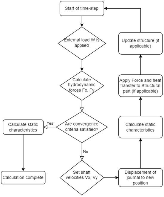
Figure 1.
Numerical model solution procedure flowchart.
3. Model Verification
It should be noted that for the purposes of this study, a hydrodynamic lubrication regime is assumed. During this steady operating condition, a generous quantity of lubricant forms a thick full film to support the external load. Researchers like Failawati et al. [19] studied the change of bearing dynamic characteristics based on different lubrication regimes, while others like de Kraker et al. [20] studied the stribeck curve for the case of WLBs. For conventional bearings such diagrams can be constructed with the help of tables, as described by Shigley et al. [21] and in other machine element designing theory literature.
For the validation of the model, three different studies are used. The study conducted by Zhang et al. [6] is used to verify the validity of the cavitation model results. The equilibrium position results are compared to the results calculated in the study of Zhou et al. [3] and the experimental validation is based on the results measured by Brito et al. [11,12]. The accuracy of the results of this study will be examined in comparison to the method published by Zhou [3]. In this case, the following parameters are set as shown in Table 1.

Table 1.
Parameters for journal bearing.
The equilibrium position results are displayed in Table 2. After comparing the results it is clear that the UDF solution appears to be almost the same as the one calculated by Zhou. In fact, since FLUENT works by solving the Navier–Stokes equations numerically, while Zhou utilized Reynolds’ equation, it is safe to say that the solution extracted in the present study is in fact closer to the actual case.
Table 2.
Comparison of equilibrium position results.
The simulation is repeated for L/D ranging from 0.5 to 1.0. In Figure 2, the equilibrium locus is calculated and compared to the one calculated by Zhou [3].
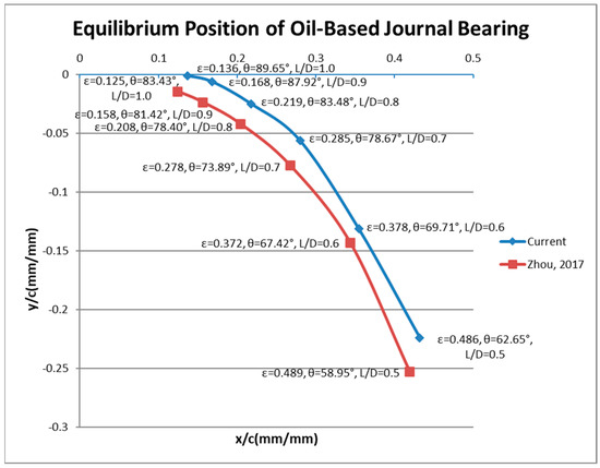
Figure 2.
Influence of bearing length (L) on the equilibrium position [3].
The equilibrium locus is also extracted for the case of a water-lubricated bearing. It is evident by observing Figure 3 that the water-lubricated bearing cannot support the same loads as easily due to the low viscosity of water.
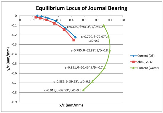
Figure 3.
Influence of bearing length (L) on the equilibrium position of water-lubricated bearings [3].
For the validation of the roughness modelling, the study made by Tauviqirrahman et al. [4] was recreated. The choice of roughness size in this particular study (and studies referenced) is unusually high yet purposefully chosen for the purposes of this study—to show with clarity and emphasize the effect of roughness on the bearing performance indicators. More specifically, a heterogenous rough surface of 25 μm roughness height was modelled with an angular velocity of 2000 rpm and an eccentricity ratio of 0.8; the below results were calculated.
Both the pressure and vapor volume fraction distributions are almost identical in contour shape as well as maximum magnitude. More specifically, Tauviqirrahman et al. [4] calculated a maximum pressure of 380 kPa and maximum vapor volume fraction of 0.832, whereas the corresponding values in this study are 376 kPa and 0.952, respectively, which is depicted in Figure 4.
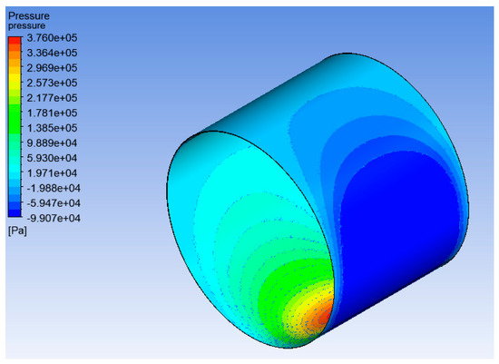
Figure 4.
Pressure distribution for roughness model validation.
It is evident, after observing Figure 5, that the cavitation effect is most intense after the pressure decrease, which, of course, is in agreement with what is known about the phenomenon.
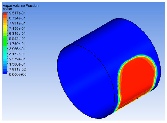
Figure 5.
Vapor volume fraction distribution for roughness model validation.
4. Results
4.1. Rough Grooved Journal Bearing
In order to have a point of reference, the geometric parameters used in the rough rigid bearing analysis will be the same ones used in the case of the elastic FSI bearing. More specifically, the geometric parameters used are listed in Table 3.
Table 3.
Geometric parameters of grooved journal bearing.
The groove number is equal to the groove radius divided by the radial clearance of the bearing. Geometric characteristics like grooves can have several benefits to the operation of journal bearings either by providing a greater supply of lubricant or by increasing certain performance indicators like the load carrying capacity. Bombos et al. [22] investigated multi-step bearings, while Gong et al. [23] studied water lubricated micro groove bearings.
It is noted that, in this study, the assumption is made that no contact between the shaft and bearing or asperities takes place. So, to ensure hydrodynamic lubrication regardless of roughness height, the bearing is modelled in a way that the final inner diameter is always 100 mm (including the roughness height).
The grid is created as per the methodology described in the numerical scheme chapter.
This bearing has been studied extensively both in simulations and experimental investigations by Brito et al. [11,12]. The grooved bearing is subjected to an external load of W = 2 kN and an angular velocity of uJ = 4000 rpm. The lubricant is set to water and a uniform roughness ranging from 0 to 100 μm is applied. The numerical scheme is modeled using the RANS equations, thus taking into consideration the occurrence of turbulence, which is especially expected in the cases where roughness is present.
In the end, the following results regarding the friction coefficient were observed.
The friction coefficient is derived from the equation
where W is the external load applied to the bearing and Ff is the force of friction and equal to
where Rb is the bearing radius and Mf is the moment of friction acting on the bearing surface, calculated using the algorithm during the solution process.
The results appear to be in line with what would be expected based on logic and with the research published on the subject. As seen in Figure 6, the values of the friction coefficient appear to steadily increase when the roughness height rises, which is expected.
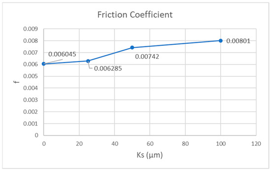
Figure 6.
Friction coefficient for various roughness values.
Figure 7 exhibits the pressure distribution for each one of the cases described above. There is a lot of interest in the fact that, while the eccentricity values increase, the maximum pressure values observed appear to decrease with every roughness increase.
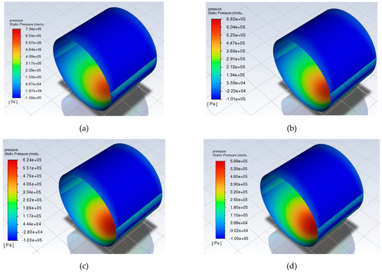
Figure 7.
Static pressure distribution for various roughness values. (a) Smooth Bearing. (b) 25 μm Roughness Bearing. (c) 50 μm Roughness Bearing. (d) 100 μm Roughness Bearing.
Tauviqirrahman et al. [4] investigated and showed in their study that the addition of a well-chosen heterogeneous rough surface can be advantageous to the tribological performance of a bearing. In this case, the same load is distributed to a larger area, since the pockets between the asperities allow a larger quantity of lubricant to be in contact with the structure. Therefore, the maximum local pressure is not as high. The change in eccentricity ratio, friction coefficient and maximum pressure with respect to roughness height is calculated and shown in Table 4 as a point of reference.
Table 4.
Rate of change of dynamic characteristics of bearing with roughness height change.
The change in the friction coefficient is as significant as expected due to the rough texturing. Even in the case of a uniform roughness surface, it is evident that the roughness height of the bearing surface is something that should be investigated very carefully during the designing and production procedure.
Figure 8 shows not only that the turbulent kinetic energy increases with respect to the roughness height but also that the turbulence is most intense at the start and end of the grooves, where the change in geometry makes the flow unsteady.
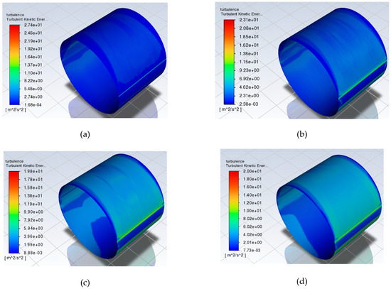
Figure 8.
Turbulent kinetic energy k distribution for various roughness values. (a) Smooth Bearing. (b) 25 μm Roughness Bearing. (c) 50 μm Roughness Bearing. (d) 100 μm Roughness Bearing.
It is important to note that the turbulent kinetic energy is greater and, thus, depicted for the outer wall of the fluid film (the bearing surface). This is expected as the geometry of the bearing surface contains the roughened texturing as well as the two axial grooves, all of which enhance the phenomenon. On the contrary, the turbulent kinetic energy is not as significant in the journal boundary layer. Figure 9 depicts the above and corresponds to the turbulent kinetic energy distribution in the inner (journal) and outer (bearing) wall, respectively. The case of 100 μm roughness is used.
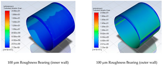
Figure 9.
Turbulent kinetic energy distribution in journal and bearing boundary layers.
The vapor volume fraction distribution is also depicted in Figure 10. The cavitation effect appears to be most prominent in the area after the upstream groove, where the pressure drops and the change in geometry makes the phenomenon much more likely to occur.
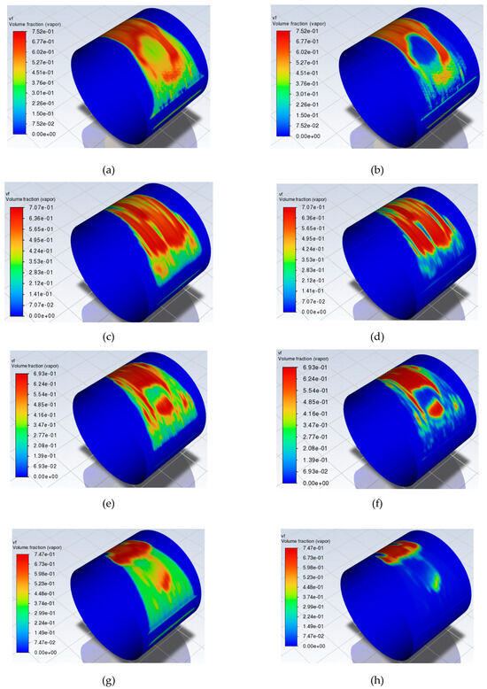
Figure 10.
Vapor volume fraction distribution for various roughness values. (a) Smooth Bearing (inner wall). (b) Smooth Bearing (outer wall). (c) 25 μm Roughness Bearing (inner wall). (d) 25 μm Roughness Bearing (outer wall). (e) 50 μm Roughness Bearing (inner wall). (f) 50 μm Roughness Bearing (outer wall). (g) 100 μm Roughness Bearing (inner wall). (h) 100 μm Roughness Bearing (outer wall).
For the case of 100 μm roughness height, Figure 11 and Figure 12 depict the turbulent dissipation rate (e) and dynamic pressure distributions, respectively. After observing the results, a connection between the grooves, turbulent effects, and cavitation is perceptible.
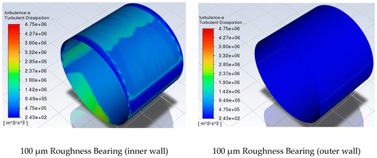
Figure 11.
Turbulent dissipation rate distribution in journal and bearing boundary layers.
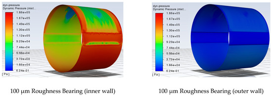
Figure 12.
Dynamic pressure distribution in journal and bearing boundary layers.
4.2. Fluid-Structure Interaction
In this section, the effect of bearing elastic deformation and thermal expansion will be investigated. Contrary to the previous section, the flow will be assumed to be laminar and the bearing surface will be smooth.
The grooved journal bearing model used is the one used by Brito [11,12]. The bush will be modeled as described by Brito and its material will be set to the widely used Thordon water-lubricated bearing material called COMPAC [24]. Although such polymers exhibit high deformation rate under load, they are often chosen for their tribological properties. Ren et al. [25] and Serdjuchenko et al. [26] also studied the behavior of non-metallic elastic WLBs. Other researchers that have provided insight on the operation of polymer-based water-lubricated bearings are Liu et al. [27], who studied WLBs operating in high angular velocities and Litwin et al. [28,29,30], who conducted experiments for several different types of materials, in order to compare the most widely used WLB materials and features, such us lubricating grooves and surface roughness. Contrary to Brito’s experiments, a load of smaller magnitude is used due to the lower viscosity of water, which makes it impossible for the water-lubricated bearing to have the same load capacity as the equivalent oil-based one. Therefore, a load of 2 kN is used instead of 10 kN. For a better comparison of the two bearings, oil-lubricated metal and water-lubricated polymer bearings, respectively, and, for verification purposes, Brito’s case is recreated (for a load of 10 kN).
Regarding the bearing geometric and physical parameters, the following model is implemented.
The bush has an inner diameter of 100 mm and the same groove characteristics as in the CFD case above. The external diameter is 200 mm and the mesh of the model is designed using hexahedral elements with 80 divisions in the axial direction, 30 in the radial direction with inflation set at the inner wall of the bush (where the FSI occurs), and 360 in the circumferential (one division per 1°). The bush material properties are provided in Table 5. Brito et al. [11,12] utilized a bush material of X22CrNi17, whereas the material COMPAC is used for the WLB case.
Table 5.
Bearing bush structure properties.
For the oil-lubricated bearing (OLB), the equivalent rigid (CFD) bearing is the one used in the experimental validation of the model.
The results calculated in comparison to the values measured by Brito et al. [11] are displayed in Table 6.
Table 6.
Comparison of grooved journal bearing model to Brito’s experimental results.
Considering the fact that the bearing structure was not modelled in the rigid bearing, the bearing surface was modelled as an isothermal wall. Still, the results in this analysis can be considered quite accurate and no unreasonable discrepancies are noted.
For the TEHD analysis of the oil-based, lubricated X22CrNi17 bearing, the eccentricity ratio is ε = 0.494803 and an attitude angle of θ = 61.81° is used. The maximum pressure calculated is Pmax = 2.72 MPa, the moment of friction is Mf = 4.37 N m, and the maximum temperature in the oil film is Tmax = 73 °C, which is only 4 °C higher than the experimental value of Tmax = 69 °C. The maximum total deformation of the bush is DLmax = 3.5 × 10⁻⁷ m = 0.35 μm, the maximum equivalent (Von–Mises) stress is σmax = 2.22 MPa, and the maximum equivalent strain is 1.009 × 10⁻⁵.
Figure 13 and Figure 14 display the pressure and temperature distribution in the oil film, respectively. The thermal effect of the grooves is once again perceptible, as a drop in temperature is evident.
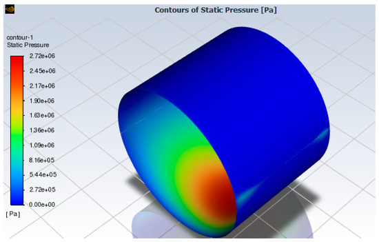
Figure 13.
Pressure distribution of oil-based grooved journal bearing in FSI analysis.
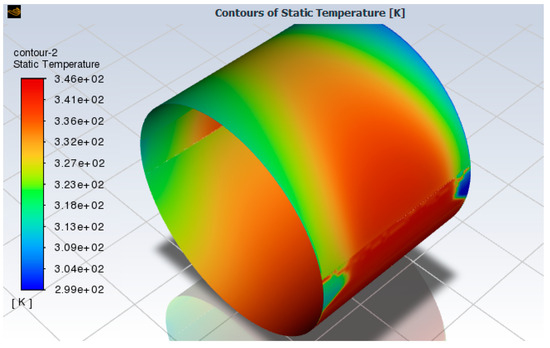
Figure 14.
Temperature distribution of oil-based grooved journal bearing in FSI analysis.
On the other hand, the equivalent WLB rigid (CFD) bearing solution is given as an equilibrium position of ε = 0.63125 and θ = 63.01°. The moment of friction is Mf = 0.73 N m and the maximum pressure is Pmax = 797 kPa
For the TEHD analysis of the water-lubricated COMPAC bearing, the eccentricity ratio is ε = 0.768136 and an attitude angle of θ = 56.17° is used. The maximum pressure calculated is Pmax = 725 kPa, the moment of friction is Mf = 0.66 N m, and the maximum temperature in the oil film is Tmax = 23 °C. The maximum total deformation of the bush is DLmax = 5.07 × 10⁻⁵ m = 50.7 μm, the maximum equivalent (von–Mises) stress is σmax = 915 kPa, and the maximum equivalent strain is εmax = 0.0015. Figure 15 and Figure 16 show the pressure and temperature distribution, respectively. It is important to note how the effect of cavitation is apparent in the temperature distribution above the upstream groove. Figure 17 also depicts the elastic deformation of the bush during operation.
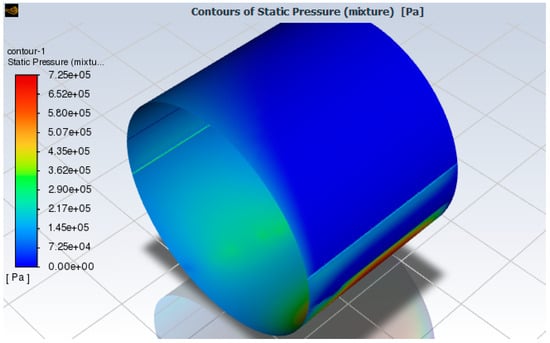
Figure 15.
Pressure distribution of grooved water-lubricated journal bearing in FSI analysis.
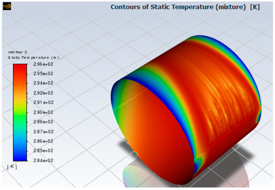
Figure 16.
Temperature distribution of grooved water-lubricated journal bearing in FSI analysis.
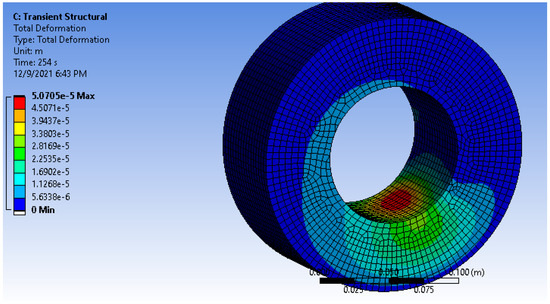
Figure 17.
Total deformation distribution in water-lubricated bush in FSI analysis.
5. Discussion
In the CFD cases, with respect to different values of surface roughness, the following results are observed.
The change in geometry is especially important in the cases where the RANS equations are implemented. Here, the phenomenon of turbulence appears.
The turbulent kinetic energy is at its maximum in the water–bush boundary layer, while it is very low in the water–journal boundary layer.
The intensity of the cavitation phenomenon is high in both the inner and outer layer of the water film. Moreover, the research findings point to the phenomenon being more prevalent in the inner layer of the water film, especially for higher roughness values. This can be associated with two factors in the flow:
- One of them is the effect of turbulence. As shown in Figure 9, the turbulent kinetic energy k is higher in the outer layer of the film, while it is minimized towards the inner layer. The logical conclusion is that the turbulent kinetic energy dissipates into heat through viscous forces and eddy production, which would make the flow erratic, cause pressure fluctuations, and lead to cavitation inception. Indeed, the results depicted in the turbulent dissipation rate (ε) distribution validate this assumption. These can be seen in Figure 11 for the case of a 100 μm rough bearing, where the turbulent dissipation rate ε distribution is shown for both the inner and outer layer of the water film.
- The other factor is the rotation of the shaft, which, coupled with the eddy production and dissipation, leads to drops in pressure and, thus, enhances the cavitation phenomenon. This assumption can be verified by investigating the dynamic pressure in the water flow, which represents the decrease in the static pressure and increase in the dynamic one, due to the velocity of the fluid. Figure 12 exhibits how the dynamic pressure is much higher in the inner layer of the water film, while it is almost non-existent in the outer one, which is of course expected as the bearing wall is stationary.
Taking the above into consideration, a kind of pattern forms. The geometry of the bearing (high surface roughness and axial grooves) coupled with the low viscosity of the water (liquid) leads to an increase in turbulent kinetic energy near the bearing surface. Energy dissipation is the outcome of turbulence. The turbulent kinetic energy leads to eddy production. The eddies interact with each other at the initial phase of dissipation, producing larger eddies. As the flow comes to rest, the eddies break down into smaller ones until such patterns are no longer present. This procedure is much more prominent in the inner wall (water–journal boundary layer), which is clearly shown in Figure 11, where the turbulent dissipation rate is much higher in the inner wall. The smooth surface and high velocity of the journal (dynamic pressure) promote a laminar flow, which explains why the dissipation rate (e) is so high at this area.
On the other hand, after observing the thermo-elastohydrodynamic analyses, it is noted that the solution of the WLB FSI (fluid–structure interaction) or TEHD analysis was affected to a high degree by the bearing bush properties. More importantly, the drop in the maximum pressure is of high interest, as the same external load can be supported more evenly. This is because the deformation forms micro pockets on the bearing surface, where the pressure can be distributed over a larger area. On the other hand, in the case of the equivalent OLB, it was observed that, although the FSI solution was closer to the experimental results measured by Brito [11], the difference was not as significant as in the case of the WLB. For that reason, there is clearly a need to be able to properly include the bearing structure into the tribological design of WLBs, since the materials from which they are made (mostly polymers) exhibit much greater elastic deformation and thermal expansion compared to their conventional bearing counterparts, which are made of metal materials. As a result, emitting the bearing deformation from the study for certain load ranges can lead to results, which, even for small external forces, might lead to large errors and uncertainty.
6. Conclusions
Several conclusions can be reached by considering the results. The addition of Vogel’s equation as well as tabular data of vaporization pressure and saturation temperature make the simulation of the flow more accurate. The larger bearing surface roughness values proved to have a negative effect on the performance of the water-lubricated bearing, since, for the same load applied (2 kN), the friction coefficient became much greater, a characteristic that is strongly associated with a loss of efficiency, a rise in temperature, and wear. Moreover, the addition of higher roughness was also proven to increase the turbulent kinetic energy k, which intensified the cavitation phenomenon. On the other hand, it is known from lubrication theory that a completely smooth surface is not ideal, since it does not allow for the formation of a thick enough oil film; consequently, a sufficient quantity of lubricant cannot become entrapped in the surface asperities and establish a stable oil wedge. It is, therefore, necessary that extra attention is given to the processing of the bearing surface during the manufacturing procedure. In the case of the FSI simulation, higher accuracy compared to the rigid (CFD) counterpart was achieved, since in the TEHD case the bush geometry and material were also modeled and, therefore, allowed thermal boundary conditions to be applied and accounted for the elastic deformation of the bush due to pressure and temperature change. The latter was proven to be of great importance in the case of water-lubricated bearings, where the bush material led to significant deformation, thus affecting the results calculated to a greater magnitude. Suggestions for further research are the study of misalignment in water-lubricated journal bearings, the use of the FSI method for studying different bush materials, and the in-depth investigation of the cavitation phenomenon in water-lubricated journal bearings. The phenomenon of mixed lubrication is also a subject of interest, while the study of bearing roughness running through the use of an FSI method would also have value for future research.
Author Contributions
Conceptualization, D.C.; methodology, D.C.; software, D.C.; validation, D.C.; formal analysis, D.C.; investigation, D.C.; resources, D.C.; data curation, D.C.; writing—original draft preparation, D.C.; writing—review and editing, D.C. and P.G.N.; visualization, D.C.; supervision, P.G.N.; project administration; P.G.N. All authors have read and agreed to the published version of the manuscript.
Funding
This research received no external funding.
Data Availability Statement
The raw data supporting the conclusions of this article will be made available by the authors on request.
Conflicts of Interest
The authors declare no conflict of interest.
Nomenclature
| Symbol | Definition | Unit |
|---|---|---|
| L | Length of bearing | m |
| D | Inner diameter of bearing | m |
| Rb | Radius of bearing | m |
| Rj | Radius of journal | m |
| e | Eccentricity | m |
| ε | Eccentricity ratio | - |
| cr | Radial clearance | m |
| θ | Attitude angle | ° |
| Φ | Bearing angle | ° |
| P | Pressure | Pa |
| uf | Angular velocity of journal | rpm |
| μ | Dynamic viscosity | Pa s |
| Cp | Thermal capacity | J/(kg K) |
| W | Journal load | N |
| Mf | Moment of friction | N m |
| Ff | Friction force | N |
| f | Coefficient of friction | - |
| g | Gravitational acceleration | m/s2 |
| Ks | Roughness height | m |
| Cs | Roughness constant | - |
| E | Modulus of elasticity | Pa |
| Su | Ultimate strength | Pa |
| v | Poisson’s ratio | - |
| w | Thermal conductivity | W/m K |
| ath | Coefficient of thermal expansion strain | 10−6/K |
| σmax | Maximum equivalent stress | Pa |
| εmax | Maximum equivalent strain | - |
| DLmax | Maximum deformation | m |
| T | Temperature | K |
References
- Hori, Y. Hydrodynamic Lubrication; Springer: Tokyo, Japan, 2006. [Google Scholar]
- Nosonovsky, M.; Bhushan, B. Green Tribology: Biomimetics, Energy Conservation and Sustainability; Springer: Berlin/Heidelberg, Germany, 2012. [Google Scholar]
- Zhou, W.; Wei, X.; Wang, L.; Wu, G. A superlinear iteration method for calculation of finite length journal bearing’s static equilibrium position. R. Soc. Open Sci. 2017, 4, 161059. [Google Scholar] [CrossRef]
- Tauviqirrahman, M.; Jamari, J.; Wicaksono, A.A.; Muchammad, M.; Susilowati, S.; Ngatilah, Y.; Pujiastuti, C. CFD Analysis of Journal Bearing with a Heterogeneous Rough/Smooth Surface. Lubricants 2021, 9, 88. [Google Scholar] [CrossRef]
- Tauviqirrahman, M.; Paryanto, P.; Indrawan, H.; Cahyo, N.; Simaremare, A.; Aisyah, S. Optimal Design of Lubricated Journal Bearing Under Surface Roughness Arrangement. In Proceedings of the 2019 International Conference on Technologies and Policies in Electric Power & Energy, Yogyakarta, Indonesia, 21–22 October 2019; pp. 1–5. [Google Scholar] [CrossRef]
- Zhang, X.; Yin, Z.; Gao, G.; Li, Z. Determination of stiffness coefficients of hydrodynamic water-lubricated plain journal bearings. Tribol. Int. 2015, 85, 37–47. [Google Scholar] [CrossRef]
- Zheng, X.B.; Liu, L.L.; Guo, P.C.; Hong, F.; Luo, X.Q. Improved Schnerr-Sauer cavitation model for unsteady cavitating flow on NACA66. IOP Conf. Ser. Earth Environ. Sci. 2018, 163, 012020. [Google Scholar] [CrossRef]
- Tamboli, K.; Athre, K. Experimental Investigations on Water Lubricated Hydrodynamic Bearing. Procedia Technol. 2016, 23, 68–75. [Google Scholar] [CrossRef]
- Xie, Z.; Li, J.; Tian, Y.; Du, P.; Zhao, B.; Xu, F. Theoretical and experimental study on influences of surface texture on lubrication performance of a novel bearing. Tribol. Int. 2024, 193, 109351. [Google Scholar] [CrossRef]
- Xie, Z.; Jiao, J.; Zhao, B.; Zhang, J.; Xu, F. Theoretical and experimental research on the effect of bi-directional misalignment on the static and dynamic characteristics of a novel bearing. Mech. Syst. Signal Process. 2024, 208, 111041. [Google Scholar] [CrossRef]
- Brito, F.P.; Bouyer, J.; Miranda, A.S.; Fillon, M. Experimental Investigation of the Influence of Supply Temperature and Supply Pressure on the Performance of a Two Axial Groove Hydrodynamic Journal Bearing. J. Tribol. 2007, 129, 98–105. [Google Scholar] [CrossRef][Green Version]
- Brito, F.P.; Miranda, A.S.; Fillon, M. Analysis of the effect of grooves in single and twin axial groove journal bearings under varying load direction. Tribol. Int. 2016, 103, 609–619. [Google Scholar] [CrossRef]
- Reynolds, O. On the Theory of Lubrication and its Application to Mr. BEAUCHAMP TOWER’S Experiments, including an Experimental Determination of the Viscosity of Olive Oil. Phil. Trans. R. Soc. 1886, 177, 157–167. [Google Scholar]
- Tower, B. First Report on Friction-Experiments (Friction of Lubricated Bearings). Proc. Inst. Mech. Eng. 1883, 34, 632–659. [Google Scholar] [CrossRef]
- Tower, B. Second Report on Friction-Experiments (Experiments on the Oil Pressure in a Bearing). Proc. Inst. Mech. Eng. 1885, 22, 58–70. [Google Scholar] [CrossRef]
- Çengel, Y.A. Thermodynamics: An Engineering Approach; McGraw-Hill Higher Education: Boston, MA, USA, 2008. [Google Scholar]
- Bhatt, C.P.; McClain, S.T. Assessment of Uncertainty in Equivalent Sand-Grain Roughness Methods. In Proceedings of the ASME 2007 International Mechanical Engineering Congress and Exposition, Seattle, WA, USA, 11–15 November 2007; Volume 8, pp. 719–728. [Google Scholar] [CrossRef]
- Kohnke, P. Ansys Theory Reference, 001242, 11th ed.; Ansys Inc.: Canonsburg, PA, USA.
- Failawati, V.; Yamin, M.; Poernomosari, S.; Naik, A.R. CFD Analysis of the Eccentricity Ratio on Journal Bearing due to Differences in Lubrication Type. J. Nov. Eng. Sci. Technol. 2022, 1, 51–56. [Google Scholar] [CrossRef]
- de Kraker, A.; van Ostayen, R.A.J.; Rixen, D.J. Calculation of Stribeck curves for (water) lubricated journal bearings. Tribol. Int. 2007, 40, 459–469. [Google Scholar] [CrossRef]
- Shigley, J.; Mischke, C.; Brown, T. Standard Handbook of Machine Design, 3rd ed.; Mc Graw-Hill: Boston, MA, USA, 2014. [Google Scholar]
- Bombos, D.; Nikolakopoulos, P. Tribological design of a multistep journal bearing. Simul. Model. Pract. Theory 2016, 68, 18–32. [Google Scholar] [CrossRef]
- Gong, J.; Jin, Y.; Liu, Z.; Jiang, H.; Xiao, M. Study on influencing factors of lubrication performance of water-lubricated micro-groove bearing. Tribol. Int. 2019, 129, 390–397. [Google Scholar] [CrossRef]
- Thordon Engineering Manual Version E2006.1; Thordon, ON, Canada, 2006; pp. 2–12.
- Ren, G. Hypo-elastohydrodynamic lubrication of journal bearings with deformable surface. Tribol. Int. 2022, 175, 107787. [Google Scholar] [CrossRef]
- Serdjuchenko, A.; Ursolov, A.; Batrak, Y. Asymptotic estimation of the fluid film pressure in non-metallic water-lubricated staved stern tube bearings. Tribol. Int. 2022, 175, 107798. [Google Scholar] [CrossRef]
- Liu, G.; Li, M. Experimental study on the lubrication characteristics of water-lubricated rubber bearings at high rotating speeds. Tribol. Int. 2021, 157, 106868. [Google Scholar] [CrossRef]
- Litwin, W. Properties comparison of rubber and three layer PTFE-NBR-bronze water lubricated bearings with lubricating grooves along entire bush circumference based on experimental tests. Tribol. Int. 2015, 90, 404–411. [Google Scholar] [CrossRef]
- Litwin, W.; Dymarski, C. Experimental research on water-lubricated marine stern tube bearings in conditions of improper lubrication and cooling causing rapid bush wear. Tribol. Int. 2016, 95, 449–455. [Google Scholar] [CrossRef]
- Litwin, W. Influence of Surface Roughness Topography on Properties of Water-Lubricated Polymer Bearings: Experimental Research. Tribol. Trans. 2011, 54, 351–361. [Google Scholar] [CrossRef]
Disclaimer/Publisher’s Note: The statements, opinions and data contained in all publications are solely those of the individual author(s) and contributor(s) and not of MDPI and/or the editor(s). MDPI and/or the editor(s) disclaim responsibility for any injury to people or property resulting from any ideas, methods, instructions or products referred to in the content. |
© 2024 by the authors. Licensee MDPI, Basel, Switzerland. This article is an open access article distributed under the terms and conditions of the Creative Commons Attribution (CC BY) license (https://creativecommons.org/licenses/by/4.0/).