Article

Combining Artificial Neural Networks and Mathematical Models for Unbalance Estimation in a Rotating System under the Nonlinear Journal Bearing Approach

by
Ioannis Tselios
and
Pantelis Nikolakopoulos
*
Machine Design Laboratory, Department of Mechanical Engineering and Aeronautics, University of Patras, 26504 Patras, Greece
*
Author to whom correspondence should be addressed.
Lubricants 2024, 12(10), 344; https://doi.org/10.3390/lubricants12100344
Submission received: 20 August 2024 / Revised: 2 October 2024 / Accepted: 4 October 2024 / Published: 6 October 2024
(This article belongs to the Special Issue Tribological Characteristics of Bearing System, 2nd Edition)

Abstract

:
Rotating systems are essential components and play a critical role in many industrial sectors. Unbalance is a very common and serious fault that can cause machine downtime, unplanned maintenance, and potential damage to vital rotating machines. Accurately estimating unbalance in rotor–bearing systems is crucial for ensuring the reliable and efficient operation of machinery. This research paper presents a novel approach utilizing artificial neural networks (ANNs) to estimate the unbalance masses in a multidisk system based on simulation data from a nonlinear rotor–bearing system. Additionally, this study explores the effect of various operating parameters on oil film stability and vibration response through a combination of bifurcation diagrams, spectrum cascades, Poincare maps, and orbit and FFT plots. This study demonstrates the effectiveness of ANNs for unbalance estimation in a fast and accurate way and discusses the potential of ANNs in smart online condition monitoring systems.

1. Introduction

Rotating machines are fundamental components of mechanical systems and are extensively utilized in various industries. The high vibration levels that can occur may cause significant damage to the machine or even lead to complete failure of the system [1]. Rotating machinery, including turbines and compressors, is crucial equipment in aeronautics, power generation, and the shipping industry. Defects and malfunctions in these machines can lead to substantial economic losses and, therefore, must be under constant surveillance and monitoring [2].
Rotor unbalance is a common fault that results in increased vibration levels and decreases the expected life of the rotating machines. The widespread use of rotating machinery in energy generation, aviation, and the marine industry indicates the importance of monitoring its operational performance. Fault diagnosis methods allow for the detection and estimation of any deviation of the operating parameters from their normal values. Rotor unbalance is a state in which the mass center of the shaft and its components is not coincident with the rotation center. In practice, achieving perfect balance in rotors is impossible due to inherent imperfections from manufacturing errors, despite the use of sophisticated machinery and strict tolerances. Therefore, rotors often have some degree of mass imbalance, leading to a synchronous excitation force that rotates with the rotor system at a frequency equal to the rotor’s spin speed [3,4]. An effective maintenance program could provide early fault detection of rotors which would reduce unplanned and costly maintenance actions. The implementation of an effective online condition monitoring system enables accurate, real-time fault prediction within the machinery [5,6].
Unbalance is a very common fault in rotating machinery, and it has been investigated thoroughly using mathematical models and signal processing techniques, such as spectrum analysis, and time–frequency analysis [7]. However, it is still very difficult to fully estimate the severity of the unbalance of the rotor system under real working conditions [8].
In the Industry 4.0 era, accurate and fast diagnosing can be achieved by leveraging machine learning techniques alongside model-based monitoring systems. Compared to signal-based systems, model-based monitoring provides more precise and quicker information, as it incorporates prior knowledge of the vibration system into the fault identification process [9].
Journal bearings are widely used to support rotors in a variety of applications and industries. Hydrodynamic journal bearings are very common and have been used in various industries, mainly due to their reliability and high load capacity. However, due to the complex dynamic coupling between the rotating shaft and the bearing (fluid media), it is very important to study the vibration behavior under various operating conditions [10,11]. The instability of rotor–bearing systems is a critical issue, as it can lead to performance degradation, a high vibration level, and potential failure. Understanding and analyzing the parameters contributing to rotor–bearing system instability is essential for ensuring the reliable and safe operation of rotating machinery [12,13].
It would be very beneficial to consider the nonlinear aspects of vibration in unbalance analysis, since this approach can improve the efficiency of balancing process. Unfortunately, there are not a lot of research works that have developed balancing procedures considering the nonlinear vibration conditions and have practical applications, as reported in [14]. Linear models and synchronous response are generally adequate to analyze rotors supported by hydrodynamic bearings for certain operating conditions. Hence, stiffness and damping coefficients can provide an accurate model for a wide range of situations. However, in certain instances, this approach proves inadequate in capturing the dynamic behavior of the rotor–bearing system [15]. At specific rotation speeds, the perturbed motion of the rotor is no longer small, and the linear model is insufficient for analyzing the nonlinear dynamic behavior of the rotor–bearing system.
When the shaft rotates at a low rotating speed, only synchronous vibrations with minor amplitudes occur. These synchronous vibrations are caused by the unbalance forces acting on the rotor. As the rotation speed increases, the unbalance-induced vibration is not the only regime of motion. Along with synchronous vibrations, sub-synchronous vibration occurs due to oil whirl and oil whip phenomena. Oil whirl is the rotor lateral forward precessional subharmonic vibration around the center of the bearing. The amplitudes of oil whirl are higher compared to those of synchronous vibrations. As the rotation speed approaches double the value of the rotor’s first critical speed, the oil whirl pattern becomes replaced by an oil whip—a lateral forward precessional subharmonic vibration of the rotor. Oil whip maintains a constant frequency independent of rotation speed, close to the first natural frequency of the rotor, with amplitudes exceeding those of both synchronous vibrations and oil whirl [16].
Oil film instability induces high vibration in large rotating machinery mounted on hydrodynamic bearings, constraining the reliable and efficient operation of rotating systems. Consequently, it becomes a substantial issue for industries, and it is rather necessary to obtain a comprehensive understanding of the mechanism to offer effective technical support in diagnosing system malfunctions related to oil whirl/whip [17]. As a result, representative mathematical models, including the use of nonlinear forces in bearing modeling, have been developed to simulate the vibration response for the specific working conditions of such systems [18]. In recent years, there has been a growing research interest in multidisk rotating systems under the nonlinear bearing approach. Hui Ma et al. [19] investigated how the eccentric phase difference between two disks influences oil film instability in a rotor–bearing system. They employed a model using lumped masses for the rotor system, with the journal bearings simulated using a nonlinear oil film force model based on the assumption of short bearings. The study revealed that the threshold for oil film instability increased with the growth of the eccentric phase.
Amaroju Kartheek et al. [20] propose a design strategy to reduce the response of a flexible shaft supported on hydrodynamic bearings. The control strategy proposed adjusts the relative position of the unbalance masses to decrease the excitation level of the first mode. Luo et al. [21] developed a Dynamic Recurrence Index (DRI) to detect the occurrence and estimate the evolution of oil whirl in a rotating system by measuring the dynamic similarity of normal working condition and unstable operating states. Sayed H. et al. [22] study the bearing coefficients as a function of the bearing parameters based on a novel method technique of polynomial fitting.
In modern industries, maintenance is considered one of the most crucial activities, making it critical to develop improved methods for fault identification and maintenance planning. In the Industry 4.0 era, traditional fault detection methods have been sidelined in favor of online monitoring systems, which allow real-time fault estimation. This paper explores this perspective, focusing on the application of artificial neural networks. These smart systems can learn the characteristics of complex systems and give results faster than traditional methods. Artificial neural networks (ANNs) imitate biological nervous systems. The neurons (elements) of the ANN work in parallel, and they can accomplish several different functions depending on the tuning of the connection weights. Typically, ANNs are submitted to a process of adjusting connection weights known as training, with the expectation that specific inputs should lead to specific target values. The network’s training is based on the comparison of the output and the target values and is deployed until convergence is achieved. The artificial neural network is a machine learning method that has already given sufficient results not only for fault identification but also for the fast and accurate modeling of complex systems.
Reddy M.C.S. and Sekhar A.S. [23] utilize ANNs to identify unbalance and looseness in rotor–bearing systems. Mohammad Gohari and Ahmad Kord [24] investigate a model that can estimate the radius, mass, and the location of unbalance based on an ANN approach. Katsaros and Nikolakopoulos [25] combine numerical and machine learning techniques to develop a predictive tool for estimating the operating parameters of tilting pivoted pad thrust bearings. They employ the finite difference method to solve the Reynolds equation and retrieve the hydrodynamic lubrication characteristics of a pad. The innovation in this work lies in the development of a machine learning system capable of providing accurate estimation in considerably less time compared to traditional complex analyses.
The digitization of information, coupled with wide networks capable of high-speed data exchange and the availability of massive computational power, has become a crucial aspect of Rotordynamics and Mechanical Engineering as a whole. Condition monitoring of rotating machinery typically involves maintenance strategies aimed at reducing operating and maintenance costs, while ensuring maximum operating time and achieving the highest possible production rate.
The main novelty of the current work is the development of an online unbalance monitoring system based on an artificial neural network and nonlinear mathematical models that offers higher accuracy and significantly increases the performance and the maintenance activities of rotating systems.
The key novelty points of this work are the following:
  • Vibration Response Prediction: Utilization of coupled mathematical models to predict the vibration response of a rotor supported by nonlinear journal bearings.
  • Investigation of Critical Parameters: Investigation of the effect of essential factors, such as lubricant temperature and rotation speed, on the rotor’s vibration response.
  • ANN Development: Development of an artificial neural network (ANN) to estimate the unbalance masses, considering the effect of oil temperature on the bearing.
This paper is organized into six sections. Following this introduction, Section 2 focuses on developing the nonlinear mathematical models of a rotating system with two disks and presents the numerical integration methods. In Section 3, using the nonlinear models, the influence of several factors on the vibration response is investigated using the appropriate nonlinear metrics like Poincare maps, bifurcation diagrams, waterfall plots, and orbit and FFT plots. In Section 4, the ability of ANNs to perform unbalance estimation prediction under various conditions is evaluated using simulation data. Lastly, Section 5 and Section 6 are the Discussion and Conclusions Sections.

2. Mathematical Analysis of Nonlinear Rotor–Bearing System

2.1. Presentation of Rotor–Bearing System

In a fully balanced rotating system and at rotation speeds below critical speed, the only mode of motion is the rotor spinning at its operating speed. An unbalance force will push the shaft to orbit around its equilibrium point [26]. The unbalance force is a centrifugal force: F u = m u r u ω 2 e j ( ω t + φ ) , where m is the unbalance mass, r is the unbalance radius, ω the rotation speed, and φ the angle of unbalance mass. In Figure 1, the rotor-bearing system that will be analyzed is depicted and in Table 1, the properties of this rotating system are presented.
The properties of the rotor–bearing system are presented in the following table.
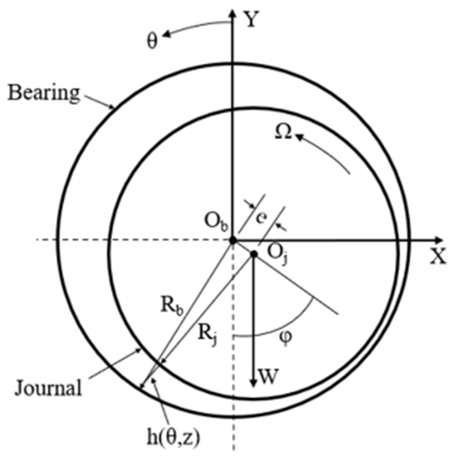
Hydrodynamic journal bearings are widely used in industry due to their simplicity, efficiency, and cost-effectiveness. The geometry of the journal bearing is shown in Figure 2, where Ob is the center of the bearing, Oj is the journal center, Rb is the bearing radius, Rj is the journal radius, and e is the bearing eccentricity. The eccentricity ratio is defined as ε = e C , where C is the radial clearance.
The instability of rotor–bearing systems, due to the complex dynamic coupling between the rotating shaft and the oil film of the bearing, can lead to performance degradation, a high vibration level, and potential failure. Therefore, it is very important to study the vibration behavior under various operating conditions to ensure the reliable and safe operation of the system.
As mentioned earlier, stiffness and damping coefficients, under the assumption of a linear bearing model, offer accurate predictions for many situations. However, at certain rotational speeds, the rotor’s vibration amplitude becomes significant at multiple frequencies, making the linear model inadequate for capturing the system’s behavior. Nonlinear models become necessary in regions of instability (oil whirl and whip regions), near critical speeds, and when there is a high level of unbalance in the system. Mathematical models using nonlinear bearing forces must be developed to simulate the vibration response at the above-mentioned regions.
In this study, the effect of lubricant temperature on the vibration response is also investigated, simulating realistic operating conditions of rotating machinery, as the oil film temperature increases during operation.
The hydrodynamic bearings are modeled using a nonlinear oil film force model based on short bearing theory, rather than relying on linear dynamic coefficients. This nonlinear bearing model was developed by Capone under the assumption of a short journal bearing (pressure distribution in circumference is negligible). Although this model has been in use for decades, it remains widely adopted in recent research due to its ability to provide accurate results for short journal bearings [11,20,27]. An alternative approach is solving the Reynolds equation at each time step, which offers greater precision but comes with a significantly higher computational cost.
The nonlinear journal bearing forces are produced using the Reynolds equation [27]. The dimensionless approach of Reynolds equation is as follows:
θ h 3 P θ + R b L b 2 z h 3 P z = h θ + 2 h ( Ω t )
where z = Z/Lb, h = H/C is the oil film thickness, P is the nondimensional pressure distribution P = p 6 μ Ω ( R b C ) , R b is the bearing radius, and Lb is the bearing length.
The oil film thickness H is given from the following equation:
H = C ( 1 + ε cos θ )
In the short journal bearing, the ratio of length to diameter is lower than 0.5. Ocvirk developed a solution for Equation (1) considering the short bearing approach. In this case, the pressure gradient on the circumferential direction is negligible, compared to the pressure gradient on the axial direction.
Sommerfeld half-bearing conditions are assumed under the short bearing approach and the following expression for pressure distribution arises from the Reynolds equation.
p ( θ , z ) = 1 2 ( 4 z 2 1 ) L b D b 2 ( x 2 y ˙ ) sin ( θ ) ( y 2 x ˙ ) cos ( θ ) ( 1 xcos θ   ysin θ ) 3
It is necessary to present the nondimensionalization process of the displacements and velocities of the shaft vibration. The nondimensional displacements x and y are given by the following equation:
x = X C ,   y = Y C
The nondimensional velocities x ˙   a n d   y ˙ are given by the following equation:
x ˙ = X ˙ Ω C ,   y ˙ = Y ˙ Ω C
Capone [28,29] developed a nonlinear journal bearing model for the short bearing hypothesis, which was developed by Ocvirk [30]. Mathematical expressions for reaction forces can be determined and added to the motion equation of a rotating system as an external force. By integrating Equation (1) on z from −Lb/2 to Lb/2, the oil film force by length unit in the circumferential direction is obtained. Integrating this oil film force on the circumferential direction θ from 0 to π, the vertical and horizontal forces acting on the shaft are obtained.
The oil film forces which are obtained from the short journal bearing theory can be expressed as follows:
Fb x Fb y =   μ Ω R b L b R b C 2 L b D b 2 fb x fb y
fb x fb y = ( x 2 y ˙ ) 2 + ( y + 2 x ˙ ) 2 0.5 1 x 2 y 2 3 xV ( x , y , α ) sin α   G ( x , y , α ) 2 cos α   S ( x , y , α ) 3 yV ( x , y , α ) + cos α   G ( x , y , α ) 2 sin α   S ( x , y , α )
V ( x , y , α ) = 2 + ( ycos α xsin α ) G ( x , y , α ) 1 x 2 y 2
S ( x , y , α ) = xcos α + ysin α 1 ( xcos α + ysin α ) 2
G ( x , y , α ) = 2 ( 1 x 2 y 2 ) 0.5 π 2 + arctan ycos α   xsin α ( 1 x 2 y 2 ) 0.5
α = arctan y + 2 x ˙ x 2 y ˙ π 2 sign y + 2 x ˙ x 2 y ˙ π 2 sign y + 2 x ˙
The mathematical model of the rotor bearing system is divided into two parts: the finite element model of the shaft and the disks, and the nonlinear hydrodynamic forces from the bearings, which are obtained by solving the Reynolds equation under the short bearing theory. The differential equation of motion for the nonlinear analysis of the system is given by Equation (12), which considers the hydrodynamic force, the unbalance forces, and the rotor weight.
M u ¨ + C + Ω G + β rid [ K ] u ˙ + ( K + β rid Ω [ Κ rid ] ) u = F b + F u + W
  • M ,   Mass   matrix ;
  • C ,   Damping   matrix ;
  • G ,   Gyroscopic   matrix ;
  • Ω ,   the   rotation   speed   of   the   rotor ;
  • K ,   Stiffness   matrix ;
  • K rid ,   Stiffness   matrix   for   Rotor   Internal   Damping   contribution ;
  • β rid ,   Rotor   Internal   Damping   coefficient ;
  • u = { x   y   θ   ψ } ,   Displacement   vector ;
  • F b ,   Nonlinear   bearing   force   vector ;
  • F u ,   Unbalance   force   vector ;
  • W ,   Weight .
The full matrices of the system consist of the sum of the matrices of the shaft, the disks, and the bearings. It is well known that Rotor Internal Damping produces non-conservative forces and can be destabilizing at some rotation speeds since it inserts power into the rotor during each revolution [31,32]. The rotor is simulated as three Timoshenko beams; each Timoshenko beam has two nodes and each node has four dofs, translation, and rotation in the horizontal and vertical directions, respectively. Disks are modeled as concentrated parameters. Bearings are introduced using the forces obtained from nonlinear bearing equations as explained earlier.
Figure 3 illustrates the difference between the linear and nonlinear approaches. As previously mentioned, linear coefficients yield accurate results for small-amplitude vibrations near the equilibrium position. In contrast, nonlinear bearing forces provide accurate results for the entire operating range. As shown in the left orbit plot, the linear dynamic bearing coefficients (K, C) accurately predict small vibration amplitudes around equilibrium position (see green line). On the other hand, the nonlinear bearing forces (see orange line in the right orbit plot) are capable of predicting fully the rotor motion even for large vibration amplitude.

2.2. Mathematical Analysis of Nonlinear Rotating System

The hydrodynamic bearings are simulated using a nonlinear oil film force model under the assumption of short bearing theory, instead of linear dynamic coefficients. Numerical integrations must be utilized to find the vibration response since the oil film force is nonlinear. Two different integration methods for the numerical solution of the ODEs were implemented, the Newmark method and the ODE23S stiff solver of MATLAB, which is based on a modified Rosenbrock formula [33]. In Section 3.2, the two methods are compared and yield similar results, demonstrating that both are robust and accurate for the vibration analysis of nonlinear systems.
In order to apply the numerical integration methods, the equations of the nonlinear system must be integrated from a selected initial state. The steady-state vibration responses of the rotor on the position of bearing 1 (left) in horizontal and vertical directions are assumed to be achieved after neglecting the first 450 revolutions. It should be noted that, in the frequency spectrum, 1× represents the synchronous vibration component corresponding to the speed equal to the speed of the rotor and 0.5× denotes the whirl speed equal to half of the rotor speed [31].

2.2.1. Newmark Method

Newmark’s robust numerical time integrator is widely used to find the displacement, velocity, and acceleration values for each selected time step [34,35]. To reduce the computational time and avoid truncation errors, the dimensionless transformations are adopted as follows:
τ = Ω t , u ~ = u C
The dynamic equations of the system are expressed in dimensionless form:
Ω 2 Μ u ~ ¨ + Ω G + C u ~ ˙ + K u ~ = F b + F u + W C
substituting M = Ω 2 Μ , C = Ω ( G + C ) , K = K , w = u ~ , and F = F b + F u + W C .
The Newmark integration method is a robust algorithm used to solve nonlinear equations in the time domain. The difference format of Newmark is as follows:
w ˙ t + Δ t = w ˙ t + 1 δ w ¨ t + δ w ˙ t + Δ t Δ t
w t + Δ t = w t + w ˙ t Δ t + 0.5 a w ¨ t + a w ¨ t + Δ t Δ t 2
where δ = 0.5 and a = 0.25 are parameters depending on the precision and stability of the numerical integration and Δτ = 0.0001 sec is the integration time step.
The following formula can be derived from the above equations:
w ¨ t + Δ t = 1 a Δ t 2 w t + Δ t w t 1 a Δ t w ˙ t ( 1 2 a 1 ) w ¨ t
w ˙ t + Δ t = δ a Δ t w t + Δ t w t + 1 δ a w ˙ t + Δ t ( 1 δ 2 a ) w ¨ t
The final equations of Newmark method can be derived from all the above:
M w ¨ t + Δ t + C w ˙ t + Δ t + K w t + Δ t = F t + Δ t
K * w t + Δ t = F * t + Δ t
where
K * = 1 a Δ t 2 M + δ a Δ t C + K
F * = F t + Δ t +   1 a Δ t 2 w t + 1 a Δ t w ˙ t + 1 2 a 1 w ¨ t M + δ a Δ t w t + δ a 1 w ˙ t + δ 2 a 1 Δ t w ¨ t C

2.2.2. State Space Representation

The ODE23S stiff solver in MATLAB R2023b is widely used due to its adaptive time stepping capability, offering advantages in both accuracy and computational efficiency. The same transformations described above are also used for ODE23S. The time response of the system is obtained for each rotor speed using the inbuilt ordinary differential equation solver in MATLAB, which solves the equations in state space form. To apply the ODE23S solver, it is necessary to represent the system in state space form as follows:
q ˙ = Aq + Bf
u ˙ u ¨ = 0 I M 1 K M 1 ( C + Ω G ) u u ˙ + 0 0 0 M 1 0 W + f unb + f bear

3. Simulation Results of Nonlinear Rotor–Bearing System

3.1. Nonlinear Analysis of Rotor Vibrations

This section focuses on the effect of various parameters, like rotation speed and lubricant temperature, on the vibration response of the rotor by using bifurcation diagrams, waterfall plots, orbit plots, frequency domain plots, and Poincare maps. The rotor model for this section has an unbalance of 1 g at the left disk at a radius r = 30 mm and Rotor Internal Damping is not taken into account (βrid = 0). The bearing length is Lb = 10 mm, bearing diameter Db = 25 mm, viscosity μ = 0.1 Pas, and bearing radial clearance C = 100 μm.
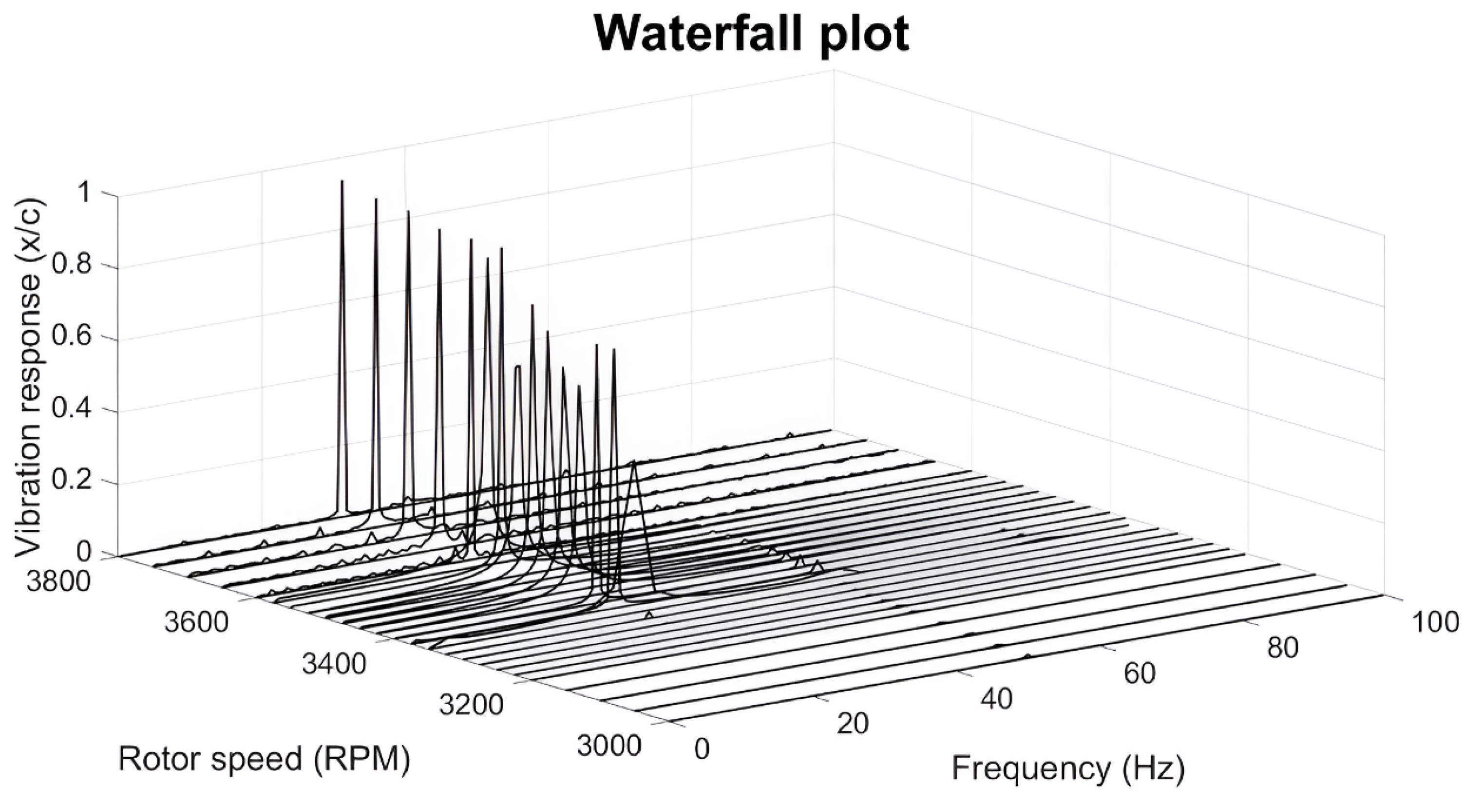
The waterfall plot of the rotor system is shown in Figure 4 for unbalance m = 1 g at disk 1. The high vibration response is obtained at the rotor speeds corresponding to the (first) critical speed and on oil whirl–whip regions. The critical speed is the rotational speed at which the rotor system experiences resonance, resulting in a large vibration response. This occurs when the excitation frequency (in this case the rotor speed) matches one of the natural frequencies of the system. At around 3275 rpm, oil whirl starts, and sub-synchronous vibration exists together with the synchronous unbalance response. At 3350 rpm, the rotor inserts in the oil whip region with very high vibration amplitudes at a subharmonic frequency (oil whip locks at the resonance frequency of the system).
In Figure 4, the waterfall plot for the vibration response is depicted from 500 rpm to the rotation speed of 3800 rpm.
In Figure 5, the waterfall plot for the vibration response is illustrated from 3000 rpm to the rotation speed of 3800 rpm.

3.1.1. Poincare Map

The Poincare map is a stroboscopic picture of motion in a phase plane, and it consists of a time series at a constant interval of T (T = 2π/ω) and is used to indicate the nature of the system motion [19]. The periodicity of the motion is employed in the stroboscopic method and the “map points” can be obtained directly from the time waveform results. Thus, the trajectories will return to the suitably selected Poincare section by a time interval corresponding to the period of unbalance excitation, i.e., the rotor speed. So, the values of state parameters are extracted from the steady-state response at the corresponding time points. All the extracted points are plotted in the plane (in this paper, the x-y plane is chosen) and the Poincare maps are obtained. A change in the number and topology of map points often indicates a change in the motion mode [36]. In the case of pure synchronous motion (period-1 motion), the points in the plane points coincide with each other and only one map point exists in the Poincare map.
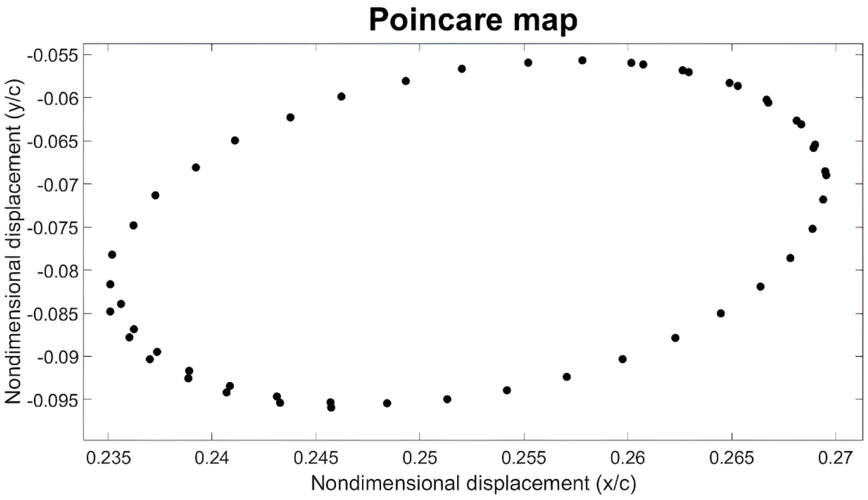
In Figure 6, Figure 7 and Figure 8, Poincare maps for speeds at oil whirl–whip regions are illustrated. In Figure 6, the Poincare map shows the start of oil whirl since there is a specific topology of map points which indicates the subharmonic vibration aspect. At lower speeds where only synchronous vibration occurs, the Poincare map would consist of only one point. The period-1 motion becomes unstable when oil whirl occurs because the synchronous motion coexists with the sub-synchronous motion.
The motion between 3275 rpm and 3350 rpm is the transition motion from oil whirl (P2-motion) to oil whip motion (quasi-periodic motion). In Figure 7, the Poincare map is illustrated for 3325 rpm and the specific topology of the map points indicates the transition from P2 to quasi-periodic motion.
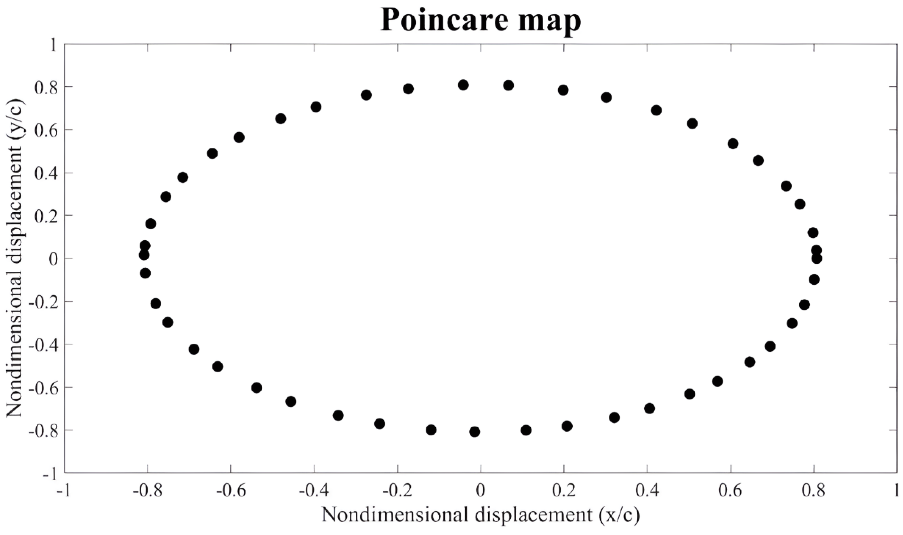
The mapping points of 3800 rpm form a closed loop in the Poincare map (Figure 8). This means the rotor motion is a pure quasi-periodic motion, since the rotor is in the oil whip region.

3.1.2. Bifurcation Analysis

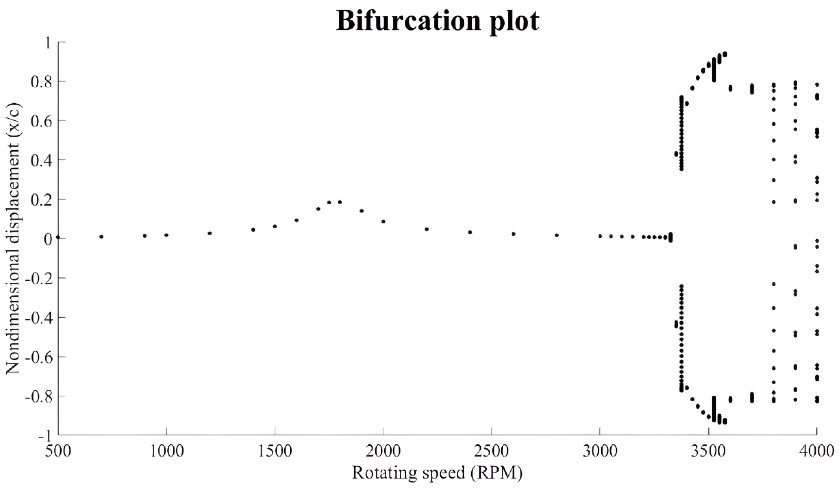
The map bifurcation diagram is obtained from Poincare map points plot at each rotating speed [36]. The bifurcation of the Poincare map can also reveal the transition from period-1 motion to quasi-periodic motion. The bifurcation map of the rotor vibration response (see Figure 9) shows that the response is a synchronous vibration with period-1 (P1 motion) from 0 to 3275 rpm where oil whirl starts to appear. At 3350–3400 rpm, oil whip (quasi periodic motion) starts to dominate the vibration and gives a high subharmonic vibration amplitude.

3.1.3. Frequency Domain Analysis

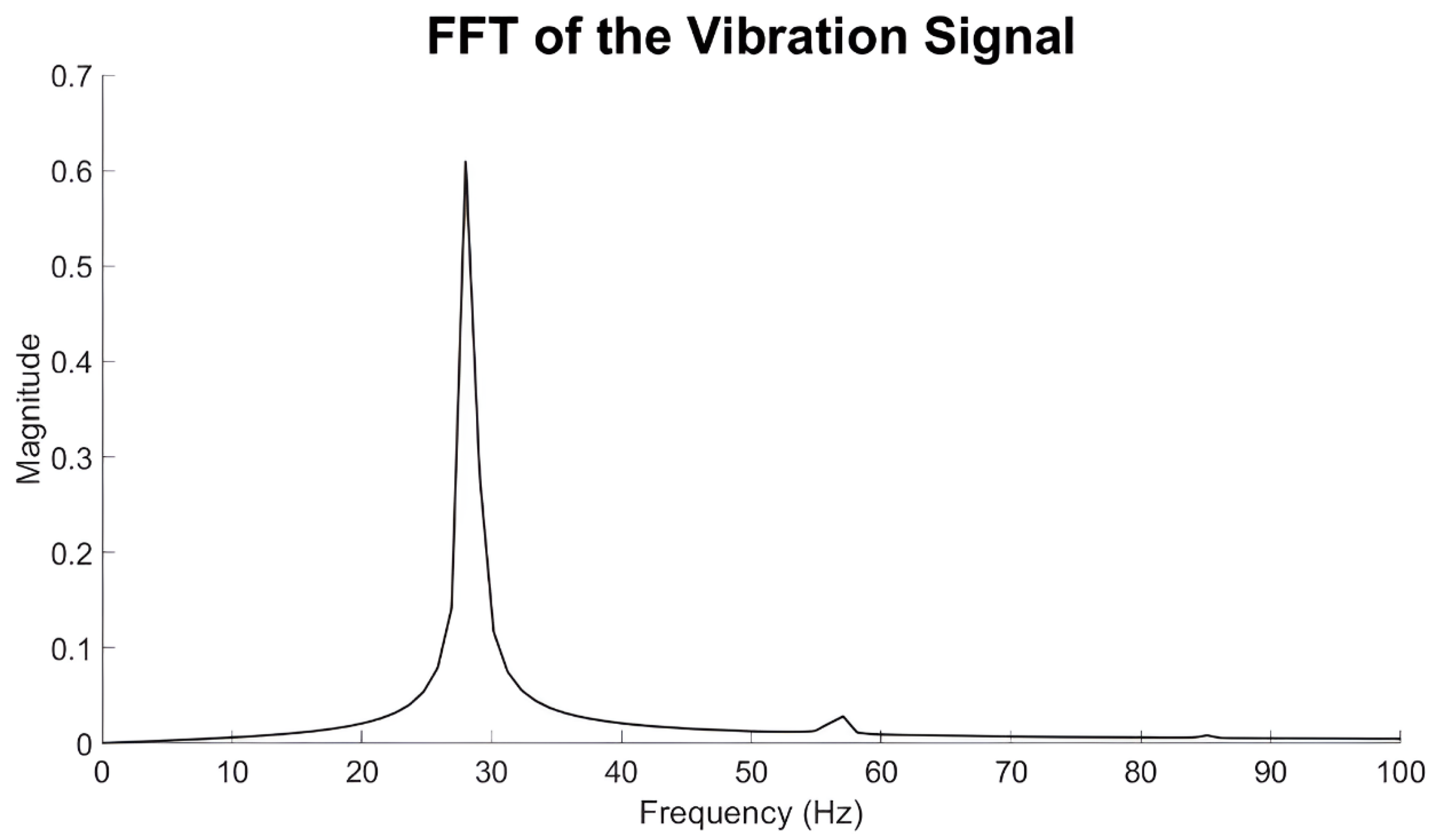
To examine in more detail the vibration response, it is appropriate to study the vibration response in the frequency domain using the Fast Fourier Transform (FFT analysis). In Figure 10, the vibration response at the frequency domain is illustrated for a rotation speed of 3200 rpm. It is clearly shown that the only source of vibration is due to unbalance for a frequency equal to the rotor speed (synchronous vibration).
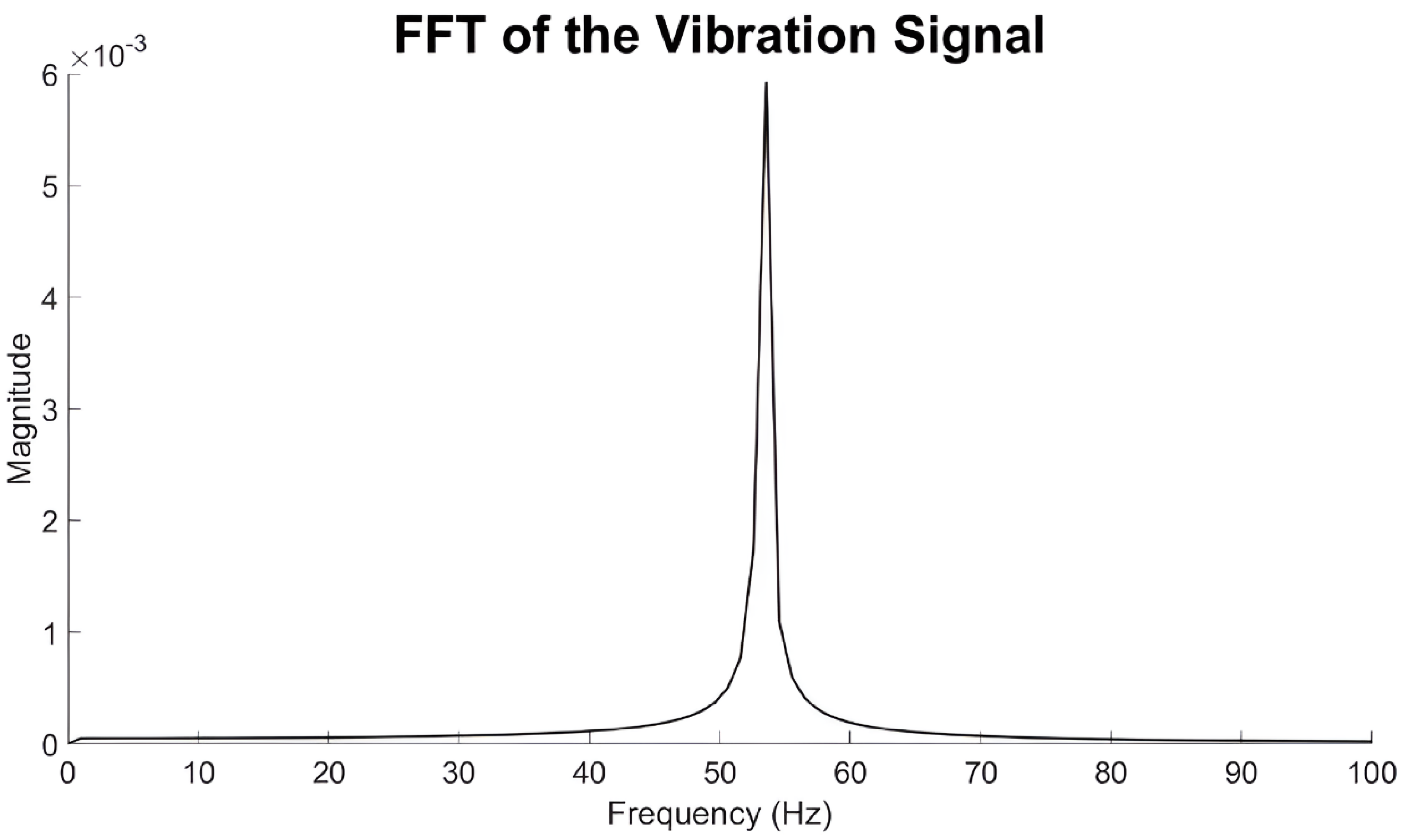
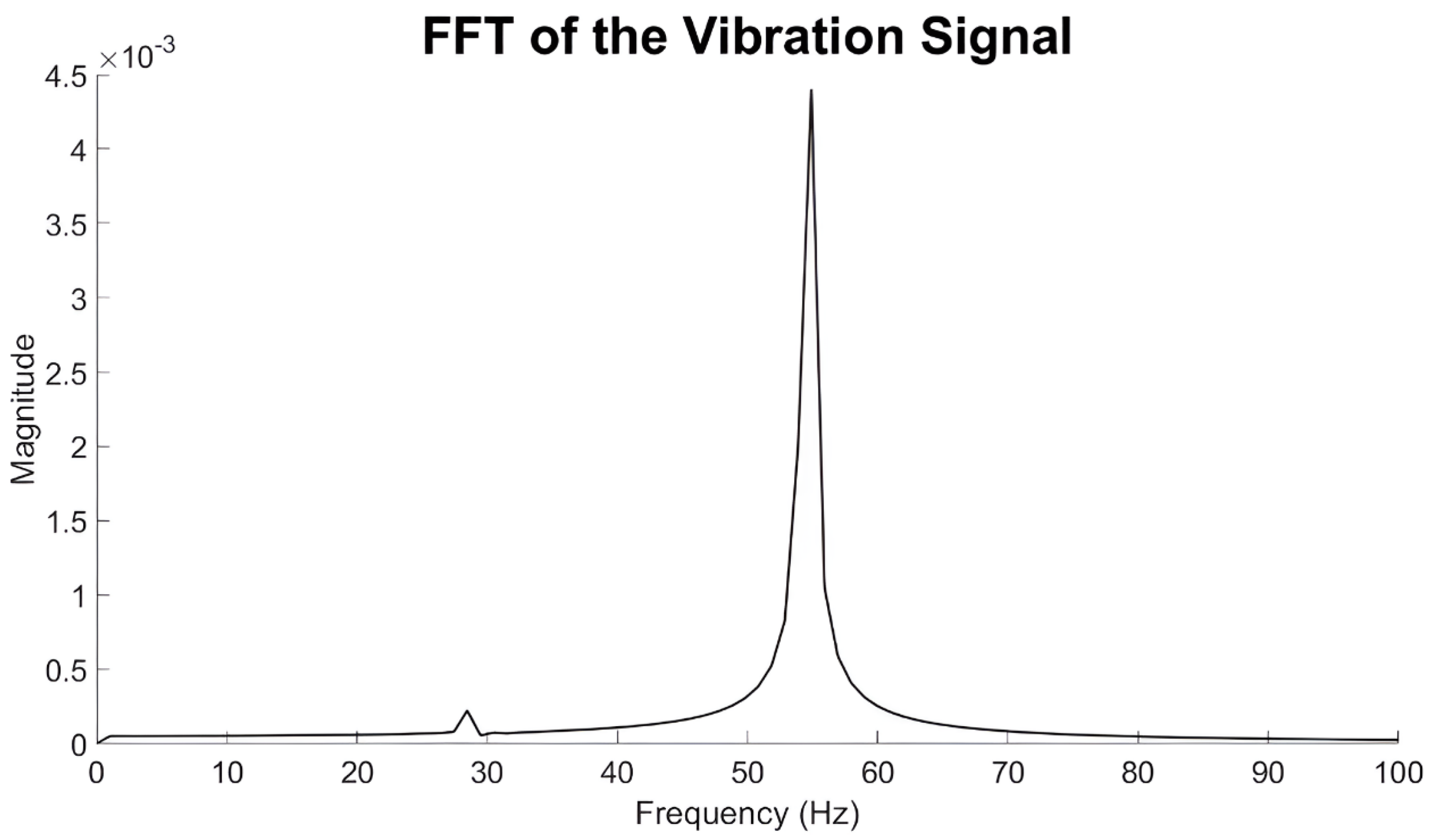
In the next diagrams, the FFT plots are illustrated for various speeds in the oil whirl–whip region to have a better understanding of the dynamics of the system. In Figure 11, it is shown that oil whirl starts at around 3275 rpm, but the subharmonic vibration magnitude is small compared to oil whip and critical speed regions. At 3275 rpm, unbalance still dominates the response, but at 3325 rpm sub-synchronous vibration starts to dominate as expected.
As shown in Figure 12, at 3325 rpm sub-synchronous vibration starts to dominate, which indicates the occurrence of oil whirl instability.
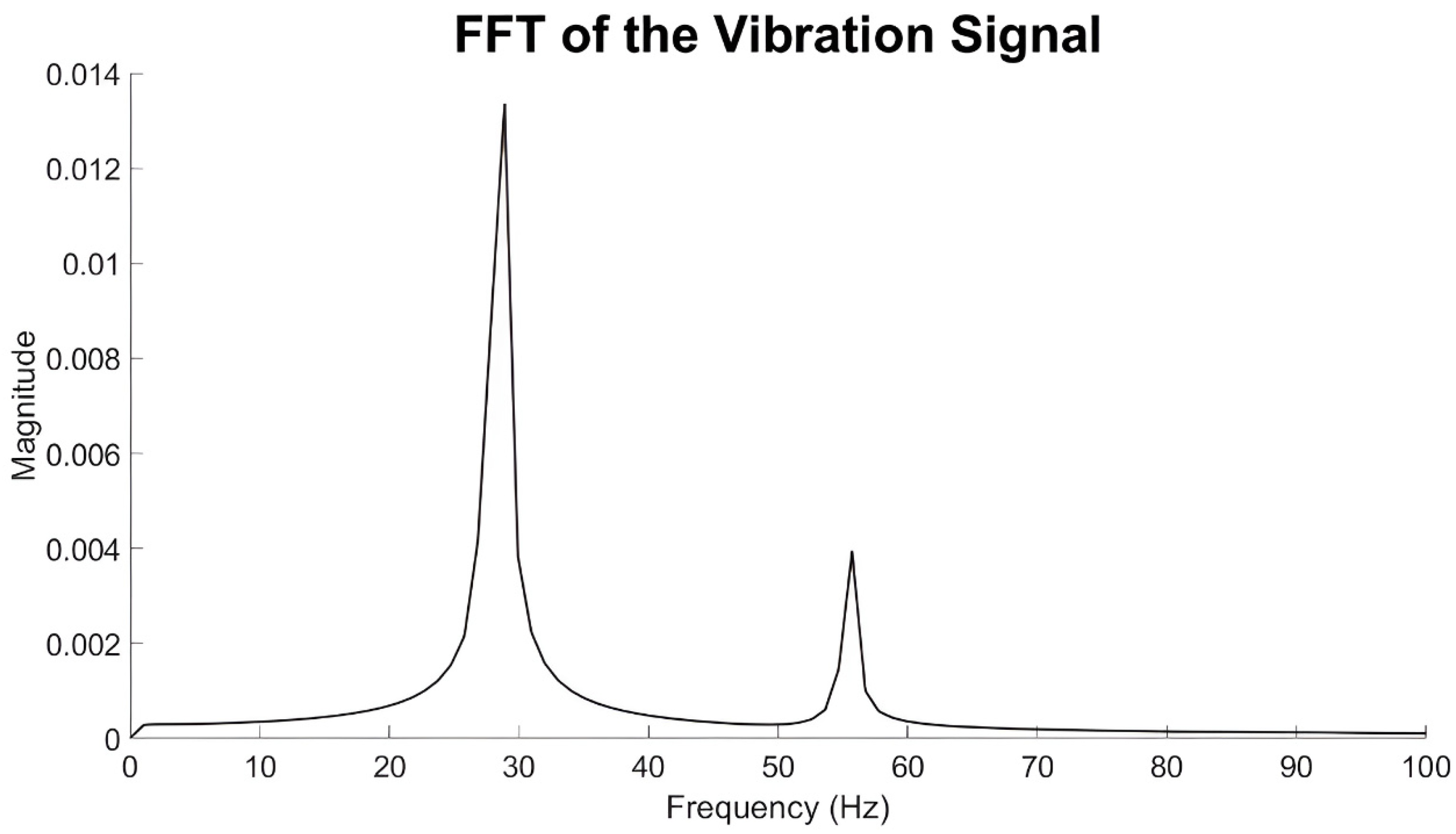
At 3400 rpm (Figure 13), the system is purely in instability—oil whip region as illustrated in the diagram below. The characteristic of oil whip is that it does not change the frequency component with rotation speed. Oil whip “locks” at the first critical speed and does not change its frequency. The amplitude of oil whip vibration is limited by the bearing clearance, but the shaft vibration may become very high at different locations (i.e., at disks). Therefore, it is important to study these aspects in order to have a better understanding of the vibration behavior of the system.

3.1.4. Orbit Plots

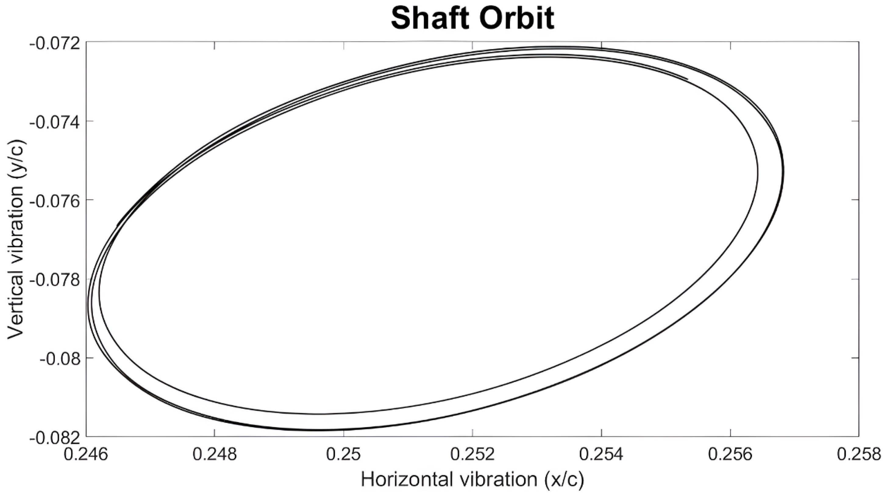
The following figures illustrate the orbits of the rotor at the left bearing position for various rotational speeds. These orbit plots provide valuable insights into the system’s vibration for evaluating the nonlinear behavior of the system.
In Figure 14, the orbit plot for the speed of 3275 rpm is depicted. This orbit scheme indicates the simultaneous presence of synchronous and sub-synchronous vibration.
In Figure 15, the orbit plot for 3300 rpm illustrates the transition from low sub-synchronous vibration (Figure 14) to a higher vibration level, as expected from oil whirl–whip theory.
In Figure 16, the orbit plot for 3700 rpm illustrates the quasi-periodic motion (oil whip region) with a very high vibration response (subharmonic vibration), close to the radial clearance of the bearing.

3.1.5. Validation of Mathematical Model

As mentioned earlier, with increasing rotational speed, unbalance-induced vibration is not the only source of vibration. In addition to synchronous motion, sub-synchronous vibrations arise due to oil whirl and oil whip phenomena. The models developed in this paper are robust and have been validated through multiple approaches. Firstly, the system’s behavior within the instability region aligns with existing research on vibration responses in the oil whirl and oil whip regions. Moreover, the system’s critical speed, approximately 1780 rpm (as indicated by the bifurcation plot), closely corresponds to the value reported by Hui Ma et al. [19] for a similar rotating system.

3.2. Comparison of Numerical Integration Methods

In Section 2, the numerical integration methods of Newmark and the ODE23S solver of MATLAB were presented and it was mentioned that both are considered very robust and accurate for nonlinear vibration response prediction. In this section, a comparative analysis of the two methods is illustrated to gain a better understanding of these numerical methodologies.
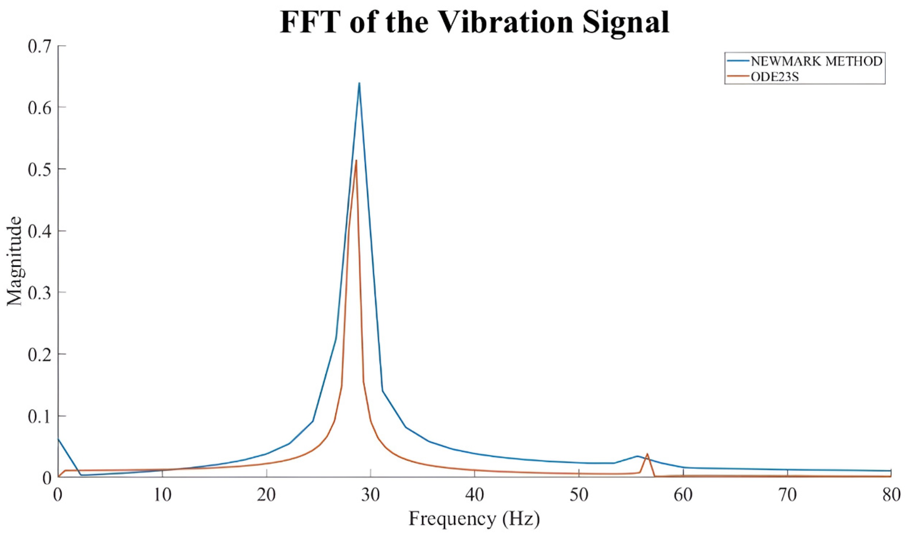
As depicted in Figure 17 and Figure 18, the two methods produce similar results even for speeds at the instability region, which indicates the capabilities and the applicability of both methods in nonlinear vibration analysis. The results of the comparative analysis indicate that the Newmark method gives a slightly lower value for oil whirl initiation compared to the ODE23S solver. In Figure 17, the FFT comparative diagram at 3400 rpm reveals that the two methodologies differ in the magnitude of subharmonic vibration. The important point of this diagram is that both methods capture the subharmonic vibration level of the system.
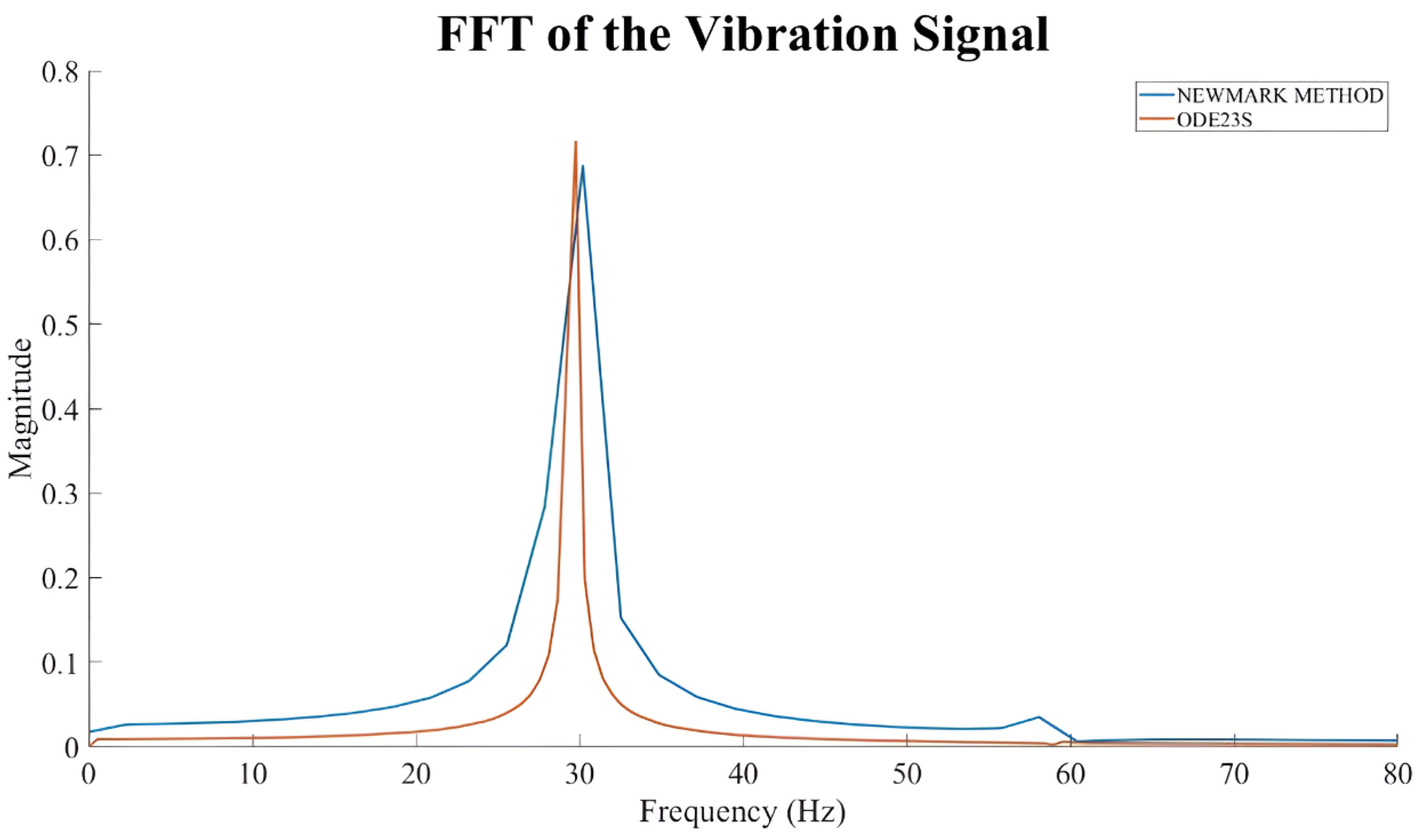
In Figure 18, the rotor is in the oil whip region, with a large vibration amplitude at a subharmonic resonance frequency (as explained earlier). The differences between the two numerical schemes are minimal, which indicates that both methodologies can efficiently represent the nonlinear effects of the rotor–bearing system.

3.3. Effect of Lubricant Temperature on Vibration Response and Necessity of Nonlinear Model

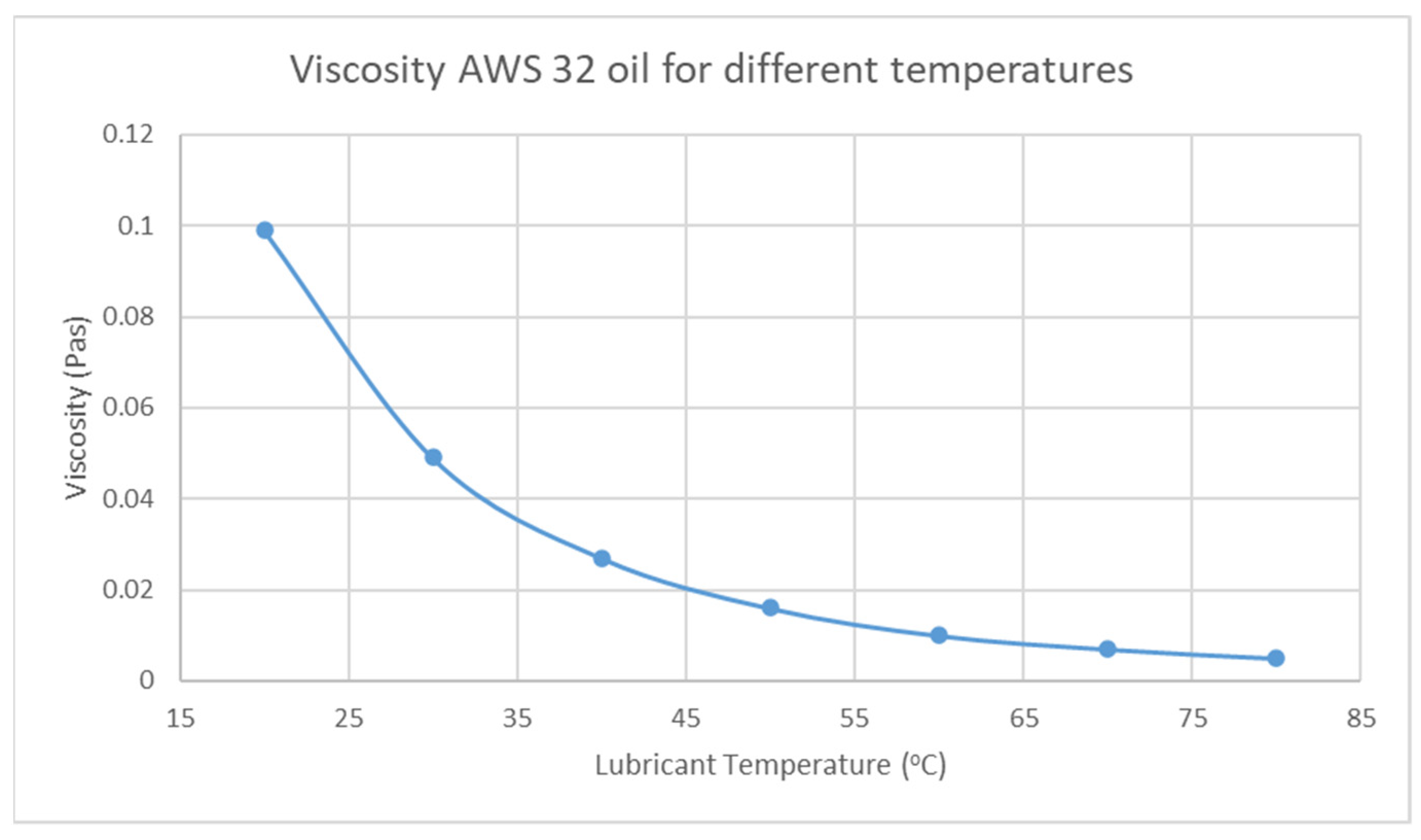
It is known that the lubricant temperature is increased for increased operation speed and time. The lubricant viscosity changes with the temperature, as depicted in Figure 19. It would be very beneficial to consider temperature effects in the vibration analysis of the rotating system, since overheating is a very common issue in rotating systems [37,38].
The lubricant is AWS 32 oil, for which there exists the following equation that describes the change in viscosity for different temperatures [39].
log [ log ( μ ) + 4.2 ] = S o log ( 1 + T 135 ) + log ( G o )
T is the temperature of the lubricant and So and Go are constants of the lubricant. For AWS 32 oil, So = 1.58 and Go = 3.98, according to Larson [40].
As mentioned earlier, nonlinear vibration models for rotor–bearing systems are necessary to study the vibration response in the oil whirl–whip regions, near critical speeds and under conditions of significant unbalance in the system. While linear dynamic coefficients of the bearing can provide accurate results, this is typically limited to cases where the vibration amplitude remains below 20% of the radial bearing clearance. Beyond this point, nonlinear mathematical models must be developed to study the vibration response of the rotor.
This section explores the effects of lubricant temperature and different unbalance masses on disk 1 in the critical speed region and specifically at a rotation speed of 1750 rpm). These parameters are studied in more detail to illustrate their influence on the system’s vibration response. To provide a clearer understanding, orbit plots of the shaft at the left bearing position will be presented in comparative diagrams.
Figure 20 presents the orbit plots of the shaft at a rotational speed of 1750 rpm for three different lubricant temperatures: 20 °C, 30 °C, and 40 °C. As expected, an increase in lubricant temperature results in a higher vibration amplitude of the rotor. The need for nonlinear modeling becomes evident, since the vibration amplitude in the critical speed region is very high. To the knowledge of the authors, the main reason for this phenomenon is that the increase in lubricant temperature reduces the damping capability of the bearing, which gives higher vibration amplitudes.
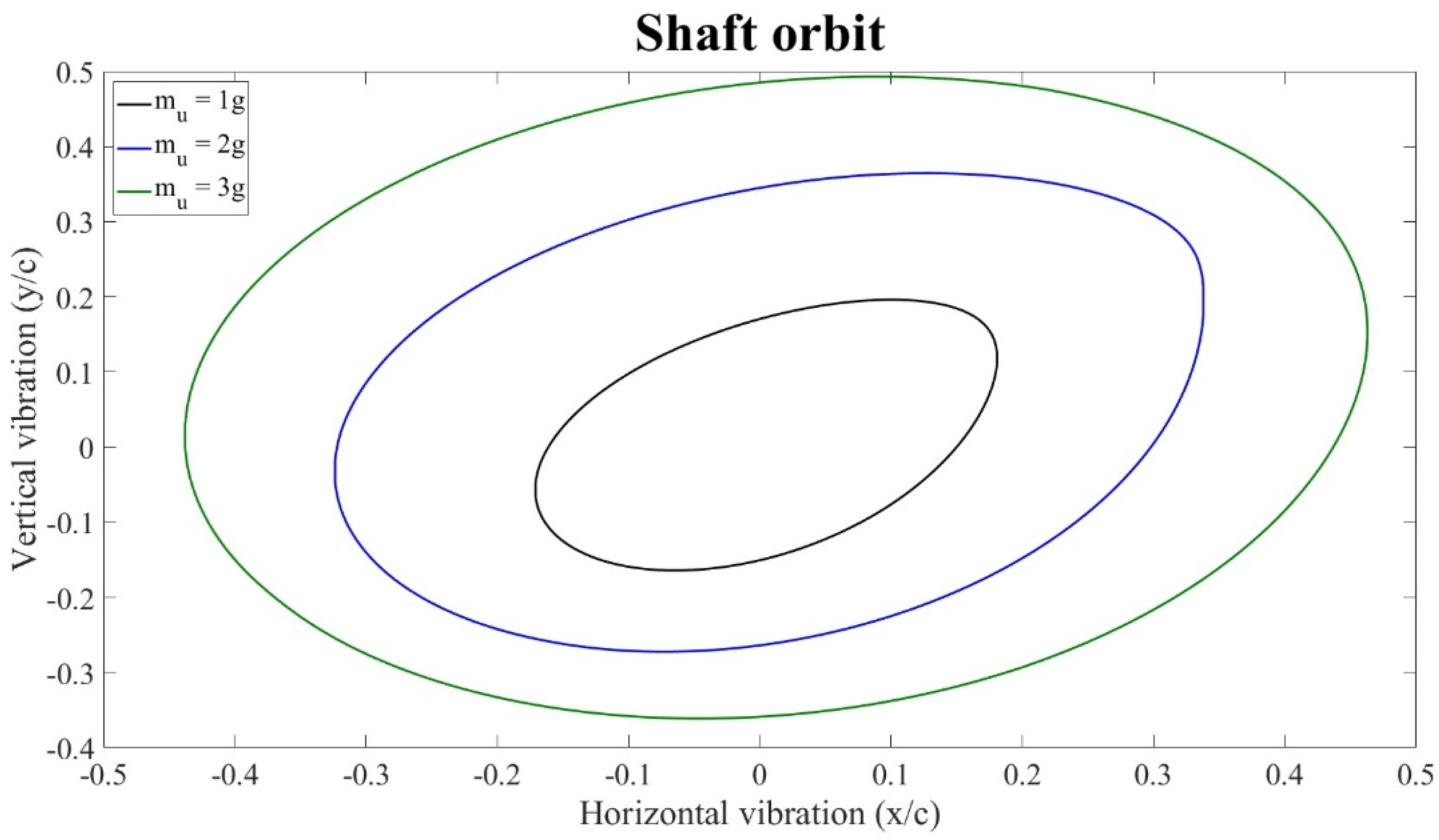
Figure 21 presents the orbit plots of the shaft at a rotational speed of 1750 rpm for three different unbalance masses on the left disk (disk 1). As expected, the increase in unbalance mass leads to a higher vibration amplitude of the rotor. The need for nonlinear modeling becomes evident, since the combination of larger unbalance and operation in the critical speed region led to a very high vibration amplitude with potential failure of the system.

4. Development of Artificial Neural Networks for Unbalance Estimation

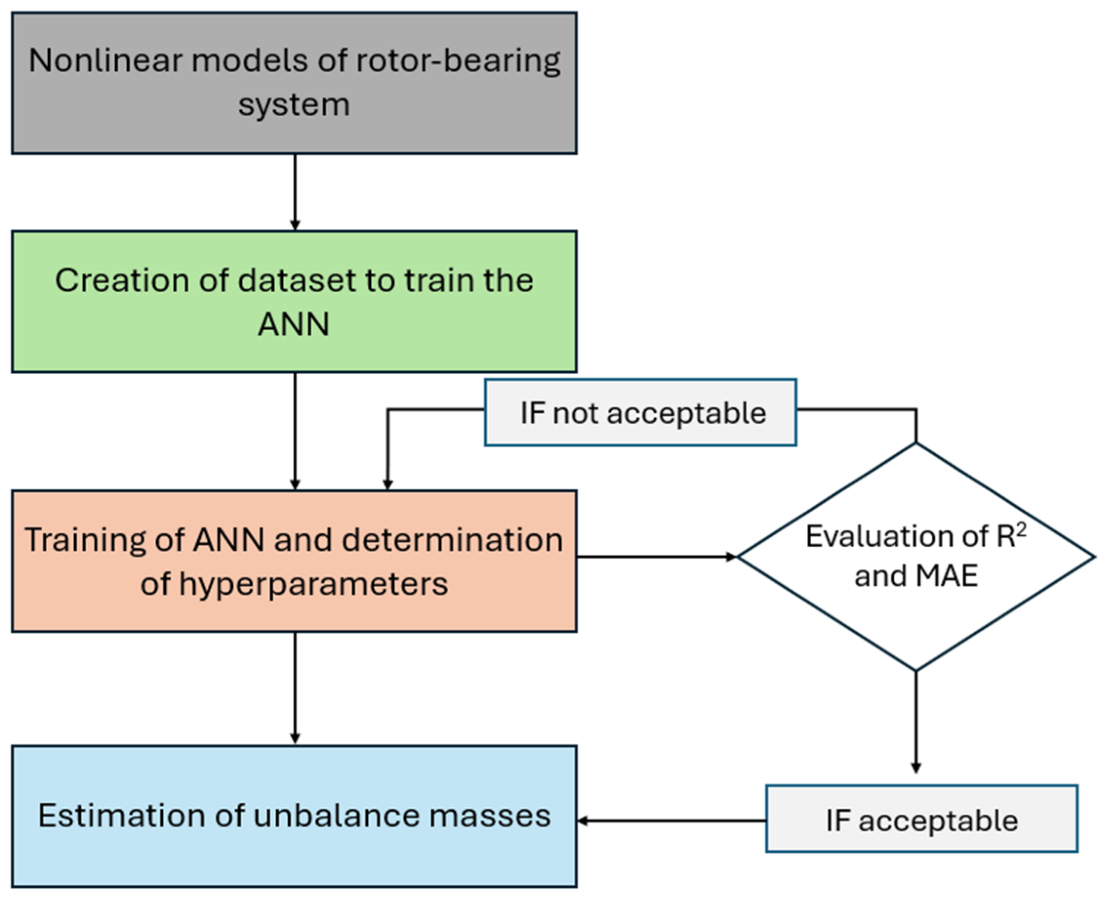
The primary objective of this section is to employ artificial neural networks (ANNs) for unbalance estimation in a rotating system using nonlinear mathematical models. A comprehensive database of vibration data is necessary in order to develop this data-driven system. The datasets are generated using the mathematical models described earlier, simulating various unbalances in the two disks for different speeds and different lubricant temperatures. The unbalance mass varies from 0.5 to 3 g at a radius r = 30 mm. The model produces two displacement vibration signals in the horizontal and vertical directions at the left bearing position. The flowchart of this research work for the development of the smart system is presented in Figure 22.
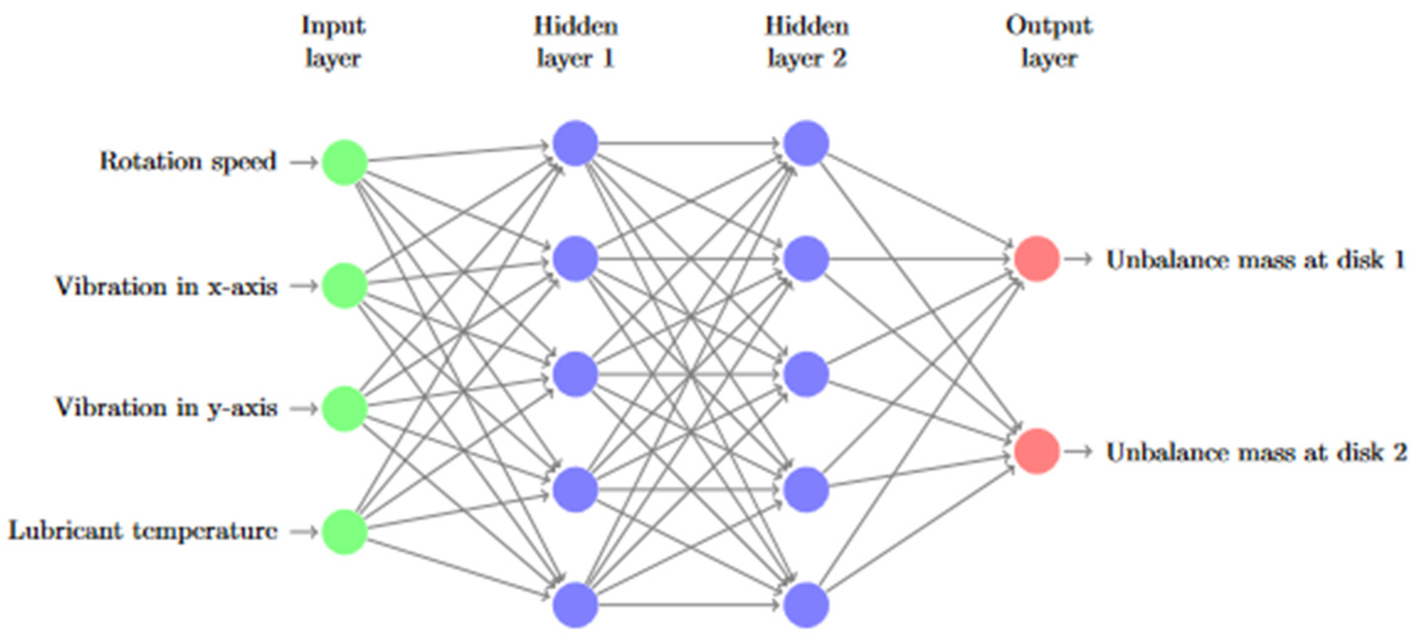
In this research work, a feed-forward multilayer perceptron (MLP) will be used due to its simplicity, short training time, and high accuracy. Figure 23 depicts the feed-forward multilayer perceptron for estimating unbalance according to rotation speed, vibration response, and lubricant temperature.
Generally, an ANN undergoes supervised training, where it is supplied with a dataset generated from the FEM model to achieve the desired network behavior.
To evaluate the performance of the regression neural network, the coefficient of determination R2 and Mean Absolute Error (MAE) will be used. A higher coefficient of determination R2 indicates a better fit, making it a useful metric for assessing the prediction capability of the model [41]. The coefficient values range between zero and one ( 0 R 2 1 ) , with the highest value indicating the best fit.
The R2 is calculated according to the following equation:
R 2 = 1 i = 1 m X i Y i 2 i = 1 m ( Y - Y i ) 2
where Xi is the target values of the dataset, Yi is the predicted values from the ANN, m is the total number of training samples, and Y ¯ is the mean of Yi values.
MAE measures the average magnitude of errors between the predicted and actual values and provides a straightforward and interpretable measure of prediction accuracy. Mean Absolute Error (MAE) is computed as follows:
MAE = 1 m i = 1 m Y i X i
where Xi is the actual values of the dataset, Yi is the predicted values from the ANN, and m is the total number of training samples.
The ANN consists of four inputs and two outputs. The inputs are the synchronous vibration amplitude (1×) in the horizontal and vertical directions in the left bearing, the rotation speed, and the lubricant temperature on the left bearing. The outputs of the network are the unbalance masses at the two disks. The loss function is the ‘mean squared error’, the optimization algorithm is ‘Adam’, the activation function for hidden layers is ReLU, and the output layer is ‘linear’. The network has two hidden layers with 30 neurons each.
The dataset for the ANN was created for different unbalances, lubricant temperatures, and rotational speeds, and the total number of samples is 15,120. In more detail, six unbalance masses at each disk were simulated (at each disk separately), for rotation speeds from 200 rpm to 3000 rpm (the value of speed is chosen to be on the safe side well below the stability threshold) with a 20 rpm step, and three lubricant temperatures of 20 °C, 30 °C, 40 °C. Of these data, 70% were used for training, 15% for validation, and 15% for testing.
In the Table 2, Table 3 and Table 4, the performance of the networks is presented using the R2 and MAE metrics for training, validation, and test segment.
The most important results are about the test segment, since the neural network is ‘tested’ with data that have not ‘seen’ before and it is a good indicator regarding the ability of the ANN to avoid overfitting and predict the desired quantities under ‘new’ conditions (input values).
Overfitting is a very common problem in machine and deep learning. The models which are over-trained on the training dataset result in weights adjusted to the ‘noise’ of the training data instead of learning “a general predicting rule” [42]. In order to achieve better performance for the networks and avoid overfitting problems, several methods were applied during the training, such as the early stopping method and feature scaling [43]. In more detail, the early stopping method stops the training after several optimization steps, leading to decreased validation loss. Feature scaling, on the other hand, is performed during the preprocessing stage and involves scaling each feature in the dataset within the range of zero to one.

5. Discussion

The implementation of artificial neural network (ANN) models for unbalance estimation using simulation data has been studied in the last few years due to the importance of unbalance faults in rotor–bearing systems. However, the unbalance estimation based on nonlinear models which also consider the lubricant temperature variation has not been studied in detail.
However, in recent years, some remarkable works integrated mathematical models and AI algorithms for fault detection but to the knowledge of the authors, there are not published works that combine these models (both AI and nonlinear mathematical models) with good accuracy for unbalance estimation. The development of a methodology for unbalance estimation using nonlinear mathematical models is the main novelty of this work since it provides very accurate results (R2 higher than 0.928 for all the outputs) and makes it feasible to incorporate it in real-time condition monitoring systems.
Future work will deal with the development of mathematical models for bearings with wear and misalignment coupled with rotordynamics models. The creation of these models will allow condition monitoring systems to perform predictions with great accuracy and for various faults in the system, significantly enhancing the performance of the rotating systems while reducing the maintenance costs.

6. Conclusions

The application of ANNs for unbalance estimation under the nonlinear bearing approach is the main novelty of this work. To develop such accurate systems, a proper and detailed nonlinear analysis of the rotating system was performed to gain a better understanding of the nonlinear dynamics. More specifically, the following are observed:
  • Nonlinear metrics like Poincare maps, bifurcation diagrams, and waterfall plots are very useful for understanding the behavior of the rotating system under various operating conditions.
  • The two different solvers, ODE23S and the Newmark method, provide similar and robust results.
  • The vibration response is affected by the lubricant temperature and rotation speed and, therefore, all these phenomena should be studied and taken into account in the simulations.
  • The utilization of artificial neural networks provides a very effective tool for online monitoring of unbalance due to fast and accurate calculation. The neural network achieves great performance (R2 is greater than 0.928 for all the outputs.)

Author Contributions

Conceptualization, P.N. and I.T.; methodology, P.N. and I.T.; writing—original draft preparation, I.T.; writing—review and editing, P.N. All authors have read and agreed to the published version of the manuscript.

Funding

This research received no external funding.

Data Availability Statement

The original contributions presented in the study are included in the article; further inquiries can be directed to the corresponding author.

Conflicts of Interest

The authors declare no conflicts of interest.

References

  1. Vázquez, J.A.; Barrett, L.E.; Flack, R.D. A Flexible Rotor on Flexible Bearing Supports: Stability and Unbalance Response. J. Vib. Acoust. 2000, 123, 137–144. [Google Scholar] [CrossRef]
  2. Chen, J.; Lin, C.; Peng, D.; Ge, H. Fault Diagnosis of Rotating Machinery: A Review and Bibliometric Analysis. IEEE Access 2020, 8, 224985–225003. [Google Scholar] [CrossRef]
  3. Shao, H.; Xia, M.; Han, G.; Zhang, Y.; Wan, J. Intelligent Fault Diagnosis of Rotor-Bearing System under Varying Working Conditions with Modified Transfer Convolutional Neural Network and Thermal Images. IEEE Trans. Ind. Inform. 2021, 17, 3488–3496. [Google Scholar] [CrossRef]
  4. Chen, X.; Wang, S.; Qiao, B.; Chen, Q. Basic Research on Machinery Fault Diagnostics: Past, Present, and Future Trends. Front. Mech. Eng. 2017, 13, 264–291. [Google Scholar] [CrossRef]
  5. Qiao, Z.; Chen, K.; Zhou, C.; Ma, H. An improved fault model of wind turbine gear drive under multi-stage cracks. Simul. Model. Pract. Theory 2023, 122, 102679. [Google Scholar] [CrossRef]
  6. Polyakov, R.; Majorov, S.; Kudryavcev, I.; Krupenin, N. Predictive Analysis of Rotor Machines Fluid-Film Bearings Operability. Vibroeng. Procedia 2020, 30, 61–67. [Google Scholar] [CrossRef]
  7. Wang, T.; Han, Q.; Chu, F.; Feng, Z. Vibration Based Condition Monitoring and Fault Diagnosis of Wind Turbine Planetary Gearbox: A Review. Mech. Syst. Signal Process. 2019, 126, 662–685. [Google Scholar] [CrossRef]
  8. Alsaleh, A.; Sedighi, H.M.; Ouakad, H.M. Experimental and Theoretical Investigations of the Lateral Vibrations of an Unbalanced Jeffcott Rotor. Front. Struct. Civ. Eng. 2020, 14, 1024–1032. [Google Scholar] [CrossRef]
  9. Wang, J.; Ye, L.; Gao, R.X.; Li, C.; Zhang, L. Digital Twin for Rotating Machinery Fault Diagnosis in Smart Manufacturing. Int. J. Prod. Res. 2018, 57, 3920–3934. [Google Scholar] [CrossRef]
  10. Mereles, A.; Alves, D.S.; Cavalca, K.L. Bifurcations and limit cycle prediction of rotor systems with fluid-film bearings using center manifold reduction. Nonlinear Dyn. 2023, 111, 17749–17767. [Google Scholar] [CrossRef]
  11. Visnadi, L.B.; De Castro, H.F. Influence of bearing clearance and oil temperature uncertainties on the stability threshold of cylindrical journal bearings. Mech. Mach. Theory 2019, 134, 57–73. [Google Scholar] [CrossRef]
  12. Ahmed, O.; El-Sayed, T.; Sayed, H. Finite element analyses of rotor/bearing system using second-order journal bearings stiffness and damping coefficients. J. Vib. Control 2023, 30, 3961–3984. [Google Scholar] [CrossRef]
  13. Eling, R.; Wierik, M.T.; Van Ostayen, R.; Rixen, D. Towards Accurate Prediction of Unbalance Response, Oil Whirl and Oil Whip of Flexible Rotors Supported by Hydrodynamic Bearings. Lubricants 2016, 4, 33. [Google Scholar] [CrossRef]
  14. Alves, D.S.; Cavalca, K.L. Investigation into the influence of bearings nonlinear forces in unbalance identification. J. Sound Vib. 2021, 492, 115807. [Google Scholar] [CrossRef]
  15. De Castro, H.F.; Cavalca, K.L.; Nordmann, R. Whirl and Whip Instabilities in Rotor-Bearing System Considering a Nonlinear Force Model. J. Sound Vib. 2008, 317, 273–293. [Google Scholar] [CrossRef]
  16. Jing, J.; Meng, G.; Yi, S.; Xia, S.-Y. On the Non-Linear Dynamic Behavior of a Rotor–Bearing System. J. Sound Vib. 2004, 274, 1031–1044. [Google Scholar] [CrossRef]
  17. Ma, H.; Wang, X.; Niu, H.; Li, H. Effects of Different Disc Locations on Oil-Film Instability in a Rotor System. J. Vibroeng. 2014, 16, 3248–3259. Available online: https://www.extrica.com/article/15094 (accessed on 15 November 2023).
  18. Alves, D.S.; Cavalca, K.L. Numerical Identification of Nonlinear Hydrodynamic Forces. In Proceedings of the 10th International Conference on Rotor Dynamics—IFToMM. IFToMM 2018; Cavalca, K., Weber, H., Eds.; Mechanisms and Machine Science; Springer: Cham, Switzerland, 2019; Volume 60. [Google Scholar] [CrossRef]
  19. Ma, H.; Li, H.; Zhao, X.; Niu, H.; Wen, B. Effects of Eccentric Phase Difference between Two Discs on Oil-Film Instability in a Rotor–Bearing System. Mech. Syst. Signal Process. 2013, 41, 526–545. [Google Scholar] [CrossRef]
  20. Kartheek, A.; Vijayan, K.; Sun, X.; Marburg, S. Stochastic Analysis of Flexible Rotor Supported on Hydrodynamic Bearings. Mech. Syst. Signal Process. 2023, 203, 110699. [Google Scholar] [CrossRef]
  21. Luo, H.; Bo, L.; Peng, C.; Hou, D. Detection and quantification of oil whirl instability in a rotor-journal bearing system using a novel dynamic recurrence index. Nonlinear Dyn. 2022, 111, 2229–2261. [Google Scholar] [CrossRef]
  22. Sayed, H.; El-Sayed, T. Nonlinear dynamics and bifurcation analysis of journal bearings based on second order stiffness and damping coefficients. Int. J. Non-Linear Mech. 2022, 142, 103972. [Google Scholar] [CrossRef]
  23. Reddy, M.C.S.; Sekhar, A.S. Identification of Unbalance and Looseness in Rotor Bearing Systems Using Neural Networks. Available online: http://www.nacomm2011.ammindia.org/files/papers/nacomm2011_attachment_183_1.pdf (accessed on 10 December 2023).
  24. Gohari, M.; Kord, A. Unbalance Rotor Parameters Detection Based on Artificial Neural Network. Int. J. Acoust. Vib. 2019, 24, 113–118. [Google Scholar] [CrossRef]
  25. Katsaros, K.P.; Nikolakopoulos, P.G. Performance Prediction Model for Hydrodynamically Lubricated Tilting Pad Thrust Bearings Operating under Incomplete Oil Film with the Combination of Numerical and Machine-Learning Techniques. Lubricants 2023, 11, 113. [Google Scholar] [CrossRef]
  26. Miraskari, M.; Hemmati, F.; Gadala, M.S. Nonlinear Dynamics of Flexible Rotors Supported on Journal Bearings—Part I: Analytical Bearing Model. J. Tribol. 2017, 140, 021704. [Google Scholar] [CrossRef]
  27. Garoli, G.Y.; De Castro, H.F. Analysis of a rotor-bearing nonlinear system model considering fluid-induced instability and uncertainties in bearings. J. Sound Vib. 2019, 448, 108–129. [Google Scholar] [CrossRef]
  28. Capone, G. Orbital motions of rigid symmetric rotor supported on journal bearings. La Mecc. Ital. 1986, 199, 37–46. [Google Scholar]
  29. Capone, G. Analytical description of fluid-dynamic force field in cylindrical journal bearing. Energ. Elettr. 1991, 3, 105–110. [Google Scholar]
  30. DuBois, G.B.; Ocvirk, F.W. The Short Bearing Approximation for Plain Journal Bearings. Trans. Am. Soc. Mech. Eng. 1955, 77, 1173–1178. [Google Scholar] [CrossRef]
  31. Friswell, M.I.; Penny, J.E.T.; Garvey, S.D.; Lees, A.W. Dynamics of Rotating Machines; Cambridge University Press: Cambridge, UK, 2010. [Google Scholar] [CrossRef]
  32. Zorzi, E.S.; Nelson, H.D. Finite element simulation of Rotor-Bearing systems with internal damping. J. Eng. Power 1977, 99, 71–76. [Google Scholar] [CrossRef]
  33. Kaps, P.; Poon, S.W.H.; Bui, T.D. Rosenbrock methods for Stiff ODEs: A comparison of Richardson extrapolation and embedding technique. Computing 1985, 34, 17–40. [Google Scholar] [CrossRef]
  34. Bathe, K. Finite Element Procedures. 1995. Available online: http://archives.umc.edu.dz/handle/123456789/116606 (accessed on 1 October 2024).
  35. Newmark, N.M. A method of computation for structural dynamics. J. Eng. Mech. Div. 1959, 85, 67–94. [Google Scholar] [CrossRef]
  36. Qian, D.; Liu, Z.; Yan, J.; Sun, L.; Wang, Y. Numerical and Experimental Research on Periodic Solution Stability of Inclined Rotor Journal Bearing System. In Proceedings of the ASME 2011 Turbo Expo: Turbine Technical Conference and Exposition. Volume 6: Structures and Dynamics, Parts A and B, Vancouver, BC, Canada, 6–10 June 2011; ASME: New York, NY, USA, 2011; pp. 321–330. [Google Scholar] [CrossRef]
  37. Golmohammadi, A.; Safizadeh, M.S. A machine learning-based approach for detection of whirl instability and overheating faults in journal bearings using multi-sensor fusion method. J. Braz. Soc. Mech. Sci. Eng. 2023, 45, 162. [Google Scholar] [CrossRef]
  38. Chang-Jian, C. Bifurcation analysis of a rotor-bearing system with temperature-dependent viscosity. J. Low Freq. Noise Vib. Act. Control 2023, 43, 75–88. [Google Scholar] [CrossRef]
  39. Alves, D.S.; Fieux, G.; Machado, T.H.; Keogh, P.S.; Cavalca, K.L. A parametric model to identify hydrodynamic bearing wear at a single rotating speed. Tribol. Int. 2021, 153, 106640. [Google Scholar] [CrossRef]
  40. Larsson, R.; Larsson, P.O.; Eriksson, E.; Sjöberg, M.; Höglund, E. Lubricant properties for input to hydrodynamic and elastohydrodynamic lubrication analyses. Proc. Inst. Mech. Eng. Part J J. Eng. Tribol. 2000, 214, 17–27. [Google Scholar] [CrossRef]
  41. Ikumi, T.; Galeote, E.; Pujadas, P.; de la Fuente, A.; López-Carreño, R. Neural Network-Aided Prediction of Post-Cracking Tensile Strength of Fibre-Reinforced Concrete. Comput. Struct. 2021, 256, 106640. [Google Scholar] [CrossRef]
  42. Dietterich, T. Overfitting and Undercomputing in Machine Learning. ACM Comput. Surv. 1995, 27, 326–327. [Google Scholar] [CrossRef]
  43. Pang, B.; Nijkamp, E.; Wu, Y.N. Deep Learning with TensorFlow: A Review. J. Educ. Behav. Stat. 2019, 45, 227–248. [Google Scholar] [CrossRef]
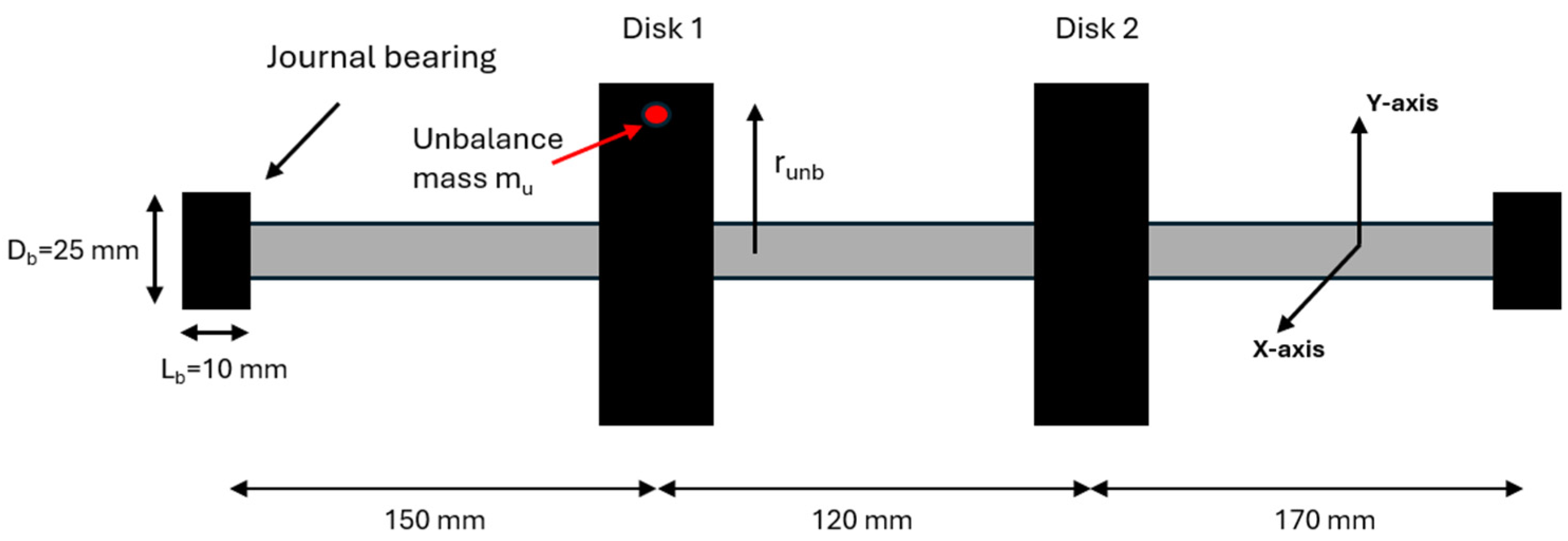
Figure 1. Rotating system supported by hydrodynamic journal bearings.
Lubricants 12 00344 g001
Figure 2. Geometry of the journal bearing.
Lubricants 12 00344 g002
Figure 3. Linear and nonlinear bearing approaches.
Lubricants 12 00344 g003
Figure 4. Waterfall plot for horizontal vibration displacement from 500 to 3800 rpm.
Lubricants 12 00344 g004
Figure 5. Waterfall plot for horizontal vibration displacement from 3000 to 3800 rpm.
Lubricants 12 00344 g005
Figure 6. Poincare map of vibration response at 3275 rpm.
Lubricants 12 00344 g006
Figure 7. Poincare map of vibration response at 3325 rpm.
Lubricants 12 00344 g007
Figure 8. Poincare map of vibration response at 3800 rpm.
Lubricants 12 00344 g008
Figure 9. Bifurcation diagram for horizontal vibration response of the rotor.
Lubricants 12 00344 g009
Figure 10. FFT of vibration signal at 3200 rpm.
Lubricants 12 00344 g010
Figure 11. FFT of vibration signal at 3275 rpm.
Lubricants 12 00344 g011
Figure 12. FFT of vibration signal at 3325 rpm.
Lubricants 12 00344 g012
Figure 13. FFT of vibration signal at 3400 rpm.
Lubricants 12 00344 g013
Figure 14. Orbit plot for 3275 rpm.
Lubricants 12 00344 g014
Figure 15. Orbit plot for 3300 rpm.
Lubricants 12 00344 g015
Figure 16. Orbit plot for 3700 rpm.
Lubricants 12 00344 g016
Figure 17. Comparison of solvers for horizontal vibration response at left bearing at 3400 rpm.
Lubricants 12 00344 g017
Figure 18. Comparison of solvers for horizontal vibration response at left bearing at 3550 rpm.
Lubricants 12 00344 g018
Figure 19. Viscosity as function of the temperature for AWS 32 oil.
Lubricants 12 00344 g019
Figure 20. Vibration amplitude at 1750 rpm for three different lubricant temperatures under 1 g unbalance mass on the left disk.
Lubricants 12 00344 g020
Figure 21. Vibration amplitude at 1750 rpm for three different unbalance masses on the left disk.
Lubricants 12 00344 g021
Figure 22. Flowchart for the development of an ANN system to estimate the unbalance masses of the rotating system.
Lubricants 12 00344 g022
Figure 23. ANN system for unbalance estimation.
Lubricants 12 00344 g023
Table 1. Properties of the rotating system.
Properties of the Rotating System
Young’s ModulusE = 210 GPa
Densityρ = 7810 kg/m3
Diameter of shaftds = 10 mm
Diameter of diskdd = 75 mm
Thickness of diskth = 25 mm
Length of shaftLs = 440 mm
Table 2. Performance metrics for the regression neural network (training segment).
Regression Neural Network
MetricsOutput 1 (m1)Output 2 (m2)
MAE0.0078 g0.0091 g
R20.9570.964
Table 3. Performance metrics for the regression neural network (validation segment).
Regression Neural Network
MetricsOutput 1 (m1)Output 2 (m2)
MAE0.0086 g0.0084 g
R20.9550.959
Table 4. Performance metrics for the regression neural network (test segment).
Regression Neural Network
MetricsOutput 1 (m1)Output 2 (m2)
MAE0.0092 g0.0075 g
R20.9280.932
Disclaimer/Publisher’s Note: The statements, opinions and data contained in all publications are solely those of the individual author(s) and contributor(s) and not of MDPI and/or the editor(s). MDPI and/or the editor(s) disclaim responsibility for any injury to people or property resulting from any ideas, methods, instructions or products referred to in the content.