Article

Skid Resistance Performance Assessment by a PLS Regression-Based Predictive Model with Non-Standard Texture Parameters

Faculty of Civil Engineering, University of Rijeka, 51000 Rijeka, Croatia
*
Author to whom correspondence should be addressed.
Lubricants 2024, 12(1), 23; https://doi.org/10.3390/lubricants12010023
Submission received: 30 November 2023 / Revised: 8 January 2024 / Accepted: 10 January 2024 / Published: 12 January 2024
(This article belongs to the Special Issue Friction Assessment in Pavement Engineering)

Abstract

:
The importance of skid resistance performance assessment in pavement engineering and management is crucial due to its direct influence on road safety features. This paper provides a new approach to skid resistance predictive model definition based on experimentally obtained texture roughness parameters. The originally developed methodology is based on a photogrammetry technique for pavement surface data acquisition and analysis, named the Close-Range Orthogonal Photogrammetry (CROP) method. Texture roughness features were analyzed on pavement surface profiles extracted from surface 3D models, obtained by the CROP method. Selected non-standard roughness parameters were used as predictors in the skid resistance model. The predictive model was developed by the partial least squares (PLS) method as a feature engineering procedure in the regression analysis framework. The proposed model was compared to the simple linear regression model with a traditional texture parameter Mean Profile Depth as the predictor, showing better predictive strength when multiple non-standard texture parameters were used.

1. Introduction

Skid resistance is one of the most significant functional properties for pavements [1]. It reflects the frictional characteristics of rough pavement surfaces in contact with vehicle tires. The importance of skid resistance performance assessment in pavement engineering and management is crucial due to its direct influence on road safety features, such as stopping distance or vehicle stability in curves. It is a physical problem in the rough contact mechanics domain theoretically explained by rubber friction theories by Persson [2,3] and Heinrich and Kluppel [4]. Both theories focus on dissipation of energy on the contact of rough and rigid pavement surface and smooth and viscoelastic vehicle tire, resulting from the hysteresis component of friction force directly related to the geometry of contact interface, i.e., pavement surface texture.
The pavement surface texture is a deviation from the true planar surface within specific wavelength and amplitude ranges defining several texture levels [5]. When pavement frictional properties are considered, two relevant texture levels are micro-texture and macro-texture [6]. It is generally acknowledged that micro-texture predominates pavement friction performance for low-speed and dry surface driving conditions, while macro-texture influences pavement friction more significantly in high-speed and wet road conditions. However, it is not recommended to exclude any of these texture levels in the analysis of skid resistance as they both have a meaningful impact on frictional performance of road surfaces [7]. In case when pavement skid resistance is observed, pavement texture is traditionally evaluated only on macro-texture level by indicators describing volumetric or geometrical properties of texture morphology. European standards recognize two main macro-texture indicators related to skid resistance: Mean Texture Depth (MTD) and Mean Profile Depth (MPD). The former is a measure of pavement texture volumetric properties evaluated by a standardized Sand Patch Test [8] and the latter is a measure of the texture’s geometrical properties calculated on pavement texture profiles, collected by following the standard [5]. These indicators describe macro-texture properties by generalizing their volumetric and geometrical properties into one single indicator [9].
Pavement surface properties related to skid resistance are evaluated on the installed pavement surface layer. This is achieved by measurement methods described in relevant standards [10,11]. In European countries, skid resistance is mostly evaluated either by static measurement method with a pendulum device or by dynamic methods with friction trailers [12]. The static method results in an approximation of road’s frictional performance for low-speed conditions, estimated from the loss of kinetic energy during the sliding process of rubber pad attached to the pendulum arm [13]. Dynamic measurement methods provide true frictional performance of inspected roads, as the measurements are carried out by devices operating at driving speeds with actual contact conditions—vehicle tire rolling and braking with a fixed or variable amount of slip.
Direct evaluation of pavement’s friction performance by any of the measurement methods has some advantages, but also several drawbacks. The main advantage is a relatively simple and straightforward evaluation of friction performance expressed as skid resistance or friction coefficient values with well-known procedures [14]. When dynamic measurement devices are used, pavement friction data are collected continuously on road network, without traffic interruption during the data acquisition. However, the frictional performance estimated from the direct measurements does not reflect the exclusive effect of the pavement surface texture. The obtained friction values result from the effect of some other influencing factors such as the operating principle of the measurement device, measurement speed, contact conditions such as temperature, presence of water or other contaminants, and material properties of bodies in contact. Therefore, the repeatability of friction measurements is possible only in very similar measurement conditions with equal measurement devices. On the other hand, pavement texture measurements provide a general description of surface roughness features specific for applied measurement procedure which are not affected by other influencing factors as friction measurements. Therefore, they represent an objective descriptor of pavement’s friction performance [7].
To overcome the drawbacks of direct estimation of friction performance, the development of a pavement friction prediction model became one of the main goals for researchers and practitioners in the field. An extensive overview of previously established prediction models and obtained results, with unique classification to simple and complex models, considering the number and type of the model’s influencing parameters was proposed in [15]. An emphasis was given to empirical models, with texture indicators being the governing influence parameters. The proposed models aimed to investigate the relationship between several influencing factors (including texture indicators) and resulting friction performance, most commonly by inferential statistical methods [16]. The proposed prediction models showed various performance, from very significant relationship between the selected texture indicator and measured friction to absence of any meaningful relationship. The results obtained by several empirical prediction models, derived from traditional texture characterization methods, are presented in the next chapter.
Recent development of optical measurement methods enabled a more detailed insight to surface roughness properties related to various physical phenomena, including friction on rough contact interface [17]. Research dealing with surface roughness features related to pavement friction exploits optical measurement methods to gain more detailed description of pavement surface properties, in comparison to the traditional measurement procedures. Texture roughness characteristics derived experimentally from advanced methods for texture analysis are being used in the friction performance predictive models overviewed in the next chapter. The results of performed research indicate a promising potential of optical methods for texture characterization in friction phenomena analysis, as the proposed models show better performance in comparison to ones developed by traditionally obtained texture roughness indicators. Some research results obtained by alternative texture characterization methods are elaborated in Section 2, where an overview of performed research in the field is presented.
The goal of this study was to propose a new model for pavement frictional performance prediction based on non-standard texture parameters, derived from an experimental pavement surface morphology analysis method Close-Range Orthogonal Photogrammetry (CROP). The CROP method utilized photogrammetry technology for texture data collection and digital surface reconstruction. The development and verification of the CROP method is thoroughly explained in [15]. Texture roughness parameters were calculated from surface profiles extracted from the digital surface models and used as predictors in the skid resistance predictive model. The main aim was to explore the potential of alternative pavement texture characterization by the CROP method for a more reliable insight to pavement texture–friction relationship in comparison to traditional texture indicators.

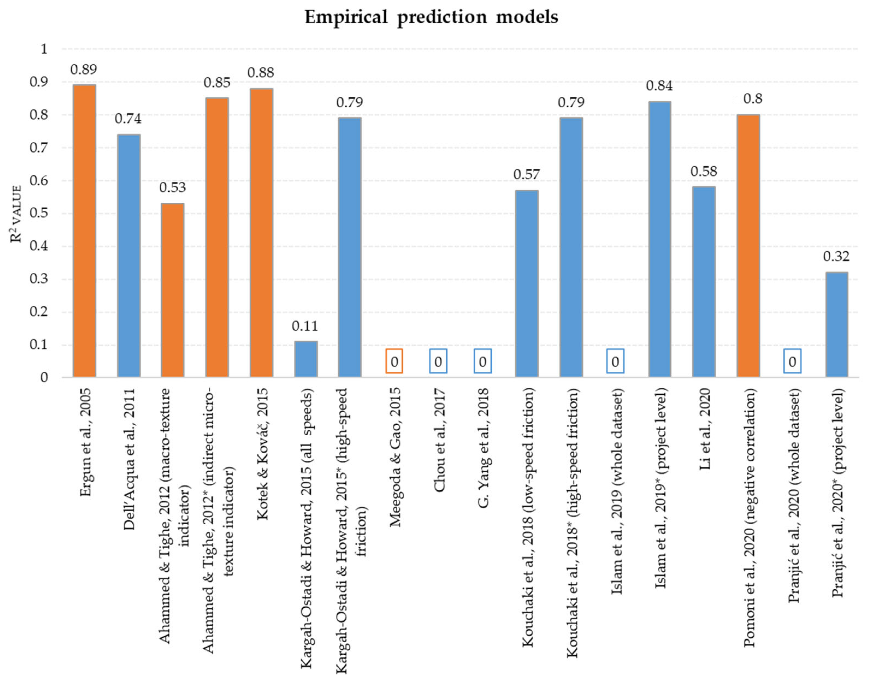
2. An Overview of Existing Prediction Models

Pavement friction predictive models are being developed in the analytical, numerical and empirical framework [14]. Analytical models follow the postulates of rubber friction theories, where the friction phenomenon is related to surface roughness, material properties and speed. The frictional response obtained from analytical models represents an approximation of actual physical phenomenon, due to the assumptions and limitations specific for applied theory. Numerical models stem from the analytical models, with the possibility of accurate representation of physical problem due to the application of numerical methods such as finite element method for non-linear problem solutions [18,19,20]. By using numerical methods for friction performance prediction, it is possible to include the true effect of each specific influencing parameter without the necessary simplifications or approximations as in the analytical models. Thus, the result of numerical models’ prediction is a highly accurate representation of real phenomenon. However, numerical models developed in the FEM framework require the discretization of contact interface, which might be a very complex task in case when surface roughness features are recognized as the main influencing parameter [14]. Empirical friction prediction models result from data collected by different experimental procedures and measurement methods, with the aim to relate measured influencing parameters with the friction performance [16]. Due to the experimental nature of research presented in this article, empirical models will be further elaborated as a basis for the development of a new prediction model.

2.1. Empirical Models Based on Traditional Texture Characterization

Empirical models aim to describe the relationship between measured influencing parameters such as texture, speed, and climatic conditions and friction performance on pavements. By following the proposed prediction model classification in [15], empirical models with one or two influencing parameters as predictors are classified as simple. Models accounting for more than two influencing parameters as predictors are categorized as complex. In this overview, special attention was given to empirical models—both simple and complex—where pavement texture indicator was considered as the main influencing parameter. Texture–friction relationship was observed exclusively or in combination with other influencing parameters.
Simple models [21,22,23,24,25,26,27] were derived from extensive pavement texture and friction measurements, performed by traditional measurement procedures defined in relevant European standards for texture measurements [5,8] and friction measurements [10,11]. Complex models [28,29,30,31,32] were derived in cases where influential parameters other than texture, such as friction measurement speed, environmental effects, and different dataset sizes, were considered in the model establishment. The predictive strength of empirical models from previous research, expressed as Pearson’s coefficient of determination R2, is given in Figure 1.
From Figure 1, it can be seen that simple prediction models showed no consistency in friction prediction, expressed in R2 values. These models were developed by using traditional texture indicator MTD and/or MPD for texture–friction relationship establishment. The obtained R2 values vary from no significant correlation for simple models [26,27,28] to moderate or even strong correlation for models [21,22,23,24,25]. By observing the obtained R2 values for complex models, it can be seen that they generally showed more consistency in friction prediction in comparison to simple models with only one or two predictors. Complex models [29,30,31] where texture indicators were complemented with other influencing parameters such as speed, pavement type or vehicle tire properties, showed better performance. However, in some cases complex models did not provide a significant texture–friction relationship despite the inclusion of additional influencing parameters in the model, such as traffic load, climatic conditions or water effect [32,33].
The analysis of existing empirical friction prediction models derived from traditionally obtained texture measurements showed that complex models considering several influencing parameters generally provide more reliable prediction of pavement friction performance in comparison to simple models with one or two traditional texture indicators as predictors. However, there is no unique trend in successful prediction of friction performance by multiple parameters models, as even some of simple models with only one predictor showed significant texture–friction correlation. In general, traditionally determined texture roughness indicators MTD and MPD were unreliable for the establishment of a meaningful texture–friction relationship. Therefore, in search for a more significant relationship between texture roughness features and friction performance of pavement surface, advanced methods for texture characterization are being implemented.

2.2. Empirical Models Based on Advanced Texture Characterization

An extension of pavement texture features description by traditional indicators became possible by using alternative methods for texture characterization, with the aim to investigate and analyze texture morphology features and provide more significant relation to friction behavior than for traditional texture parameters. For this purpose, different methodologies were explored for texture data assessment based on remote sensing and optical measurements of pavement surface with two most common technologies being photogrammetry and laser scanning [17,34]. These methods result in a realistic 3D digital representations of pavement surface morphology—digital surface models (DSMs), which can be further analyzed in a variety of texture parameters in addition to the traditional MTD and MPD indicators.
Photogrammetry is an optical measurement method utilizing digital camera for image acquisition, from which a realistic digital model of the photographed object can be reconstructed [17]. The reconstructed object consists of a large number of points with defined coordinates, utilized for further measurements and analysis of object’s geometrical features. If the distance between the object and camera is less than 300 m, photogrammetry is characterized as close range [35]. The main advantage of the photogrammetry method is the availability of data acquisition equipment. Digital cameras used for image acquisition are widely available and some research pointed out that even smartphone-integrated cameras can provide relevant results in terms of accuracy and precision of obtained digital models [36,37]. Laser scanning is another optical measurement method, where light beams are emitted from the scanner to the target surface following the triangulation principle, with known distances and angles between the light source and the sensor [38]. It is a widespread technology already in use for traditional pavement texture measurements in 2D, resulting in an MPD value as a texture indicator [39]. Recently, 3D laser scanning technology is experimentally applied for pavement surface morphology characterization, where, similar to the photogrammetry method, 3D digital surface representations are created and utilized for texture roughness analysis [40,41,42]. Laser technology enables fast collection of a relatively large database with very high precision and accurate representation of true surfaces [43]. However, the equipment is less available in comparison to the digital cameras used in the photogrammetry method, which is the main drawback of this method.
European standards [44,45] recognize and define several texture roughness parameters in the 2D and 3D domains, respectively, which are not related to any specific surface type but describe general morphology features of any rough surface. Texture parameters are grouped to describe amplitude, spatial, hybrid and material roughness features of profiles or surfaces. When analyzing pavement surface morphology, most commonly the roughness parameters are selected from the amplitude and material groups [46,47]. Advanced pavement texture characterization by roughness parameters has been utilized recently in research dealing with pavement friction performance assessment. Table 1 summarizes recent research utilizing optical measurement methods for texture roughness characterization in the establishment of friction predictive models. The focus of such studies is to determine texture-related roughness parameters from the digital representations of pavement profiles or surfaces and establish the relationship to the friction performance through a friction prediction model. Models are being developed in an empirical framework, with experimentally determined texture roughness features obtained by previously described optical measurement methods: photogrammetry or 3D laser scanning.
Research by [48] investigated the relationship between six surface-related roughness parameters in amplitude, volume and feature group determined from a photogrammetry-based data collection method and friction measurements performed by a Grip Tester device for fixed slip continuous measurements on 900 m long constructed road sections. The proposed friction predictive model was established in the multiple linear regression framework with two roughness parameters as predictors: peak material volume and peak density, describing volumetric and feature properties of top 2 mm surface roughness, respectively. The top 2 mm of analyzed pavement surface was considered as the most relevant for texture–friction phenomenon since the surface asperities on this level directly interact with the device’s measuring tire. Furthermore, research results pointed out that no significant texture–friction correlation was obtained for separate observation of micro- and macro-texture influence to friction performance. This research was performed in wet friction measurement conditions, meaning that the water film sprayed onto the surface during the measurements filled texture cavities and, therefore, could affect the obtained low correlations for texture levels below 2 mm. Another photogrammetry-based research [50] performed in laboratory on fabricated asphalt samples investigated the influence of macro-texture range roughness parameters determined from profiles extracted from digital surface models of two different asphalt pavement mixture types: five dense graded and three open graded. The developed texture analysis system produced digital surface models with resolution of 0.1 mm in horizontal and lateral plane and 0.01 mm in vertical plane. Ten roughness parameters were calculated on 100 mm long profiles, from which the micro-texture roughness features were filtered out. The effectiveness analysis of selected parameters to friction performance was performed by comparing correlation coefficients obtained between each roughness parameter and corresponding value of friction, measured by a low-speed pendulum device. The best correlation was obtained for following profile-related parameters: arithmetic mean height—Ra, root mean square wavelength lq and traditional parameter MTD. Roughness parameters extracted from open-graded asphalt mixture samples generally showed higher correlation to measured friction. The results indicated a promising perspective for texture roughness analysis by experimentally established data collection method; however, the methodology where micro-texture values were filtered out was contradictory to previous research findings. A different approach in photogrammetry application was proposed by [53], where digital surface models of pavements were utilized for profile extraction and calculation of spectral indicators as roughness descriptors. Surface images were captured by using tricolor light sources (red, green and blue). A 10 cm2 surface area was captured by the established image acquisition system and subjected to spectral analysis. The power spectral density function was calculated from the profiles and the mixture surface profile levels were calculated for different texture wavelengths. The results analysis showed that texture wavelength corresponding to the macro-texture level correlates well with the traditionally measure macro-texture indicator MTD, while texture wavelength corresponding to micro-texture level obtained significant correlation to friction performance measured by a low-speed device. This conclusion corroborated the previous research results in [48], where it was observed that texture scale separation should not be performed a priori in the analysis of texture–friction relationship.
Friction prediction models developed by texture roughness input obtained by high-end 3D laser scanning devices showed similar results, despite the advances of applied technology. Authors [49] obtained a moderate relationship between friction performance and texture features presented through texture’s fractal characterization with the Hurst exponent and the power spectral density function, calculated from surface’s digital representations generated from a 3D laser scanning device. In their predictive model, they also included traditional parameter MPD determined from digital surface model. Friction performance was determined by low-speed measurements with a pendulum device on 18 different locations. The predictive model was defined by Persson’s rubber friction theory, showing promising potential for pavement friction estimation based on surface’s fractal characteristics which supplement the traditional profile-related texture indicator. Research by [51] obtained a very strong predictive model based on surface roughness parameters from amplitude, spacing, hybrid and functional group calculated with the EN ISO 25178-2 standard. They utilized a high-end 3D laser scanning device for data acquisition and performed sensitivity analysis for determined roughness parameters to detect which are the most suitable for friction performance prediction. The friction predictive model was developed in multivariate regression analysis with six texture indicators as model predictors. Obtained values were compared to friction measurements by a high-speed dynamic device on 84 segments, showing very significant correlation with coefficient of determination of 0.95. In research by [52], roughness was examined on eighteen test sections by a 3D laser scanning device and measured by a dynamic low-speed friction measurement device. From the obtained surface scans, several parameters from amplitude, hybrid and feature group according to EN ISO 25178-2 standard were calculated, together with the fractal dimension of analyzed surfaces and traditional parameter MPD. Surfaces were processed to account only for macro-texture features and qualitatively compared to measured friction performance. The analysis showed that MPD parameter showed no significant relationship to friction, while two parameters from the feature parameters group influenced the friction performance the most. The proposed predictive model accounted for these two parameters and obtained coefficient of determination ranging from 0.76 to 0.83 with the friction values measured at different speeds. An important conclusion derived from this research is that predictive models accounting for multiple texture roughness parameters have better predictive strength than a single-predictor model. The 3D laser scanning equipment was utilized in research by [25], focusing on aggregate roughness characteristics and their influence on friction performance determined by a high-speed measurement device on 22 locations. There was no scale separation to micro- and macro-texture in roughness analysis of aggregates. In addition to friction measurements, high-speed texture measurements were also performed with traditional MPD parameter as output, differentiated on inspected locations for the type of aggregate used in pavement surface layer. The measured data were used for initial friction prediction model development, with R2 = 0.58 for MPD as a single model predictor. A multivariate linear egression predictive model was developed with aggregate roughness parameters selected from textural, amplitude, material, volume and feature parameters group after an extensive correlation analysis between the calculated parameters. The obtained coefficient of determination between measured and predicted values for the final model was 0.78, which was a significant improvement in the model’s predictive strength in comparison to preliminary model with MPD as a predictor. Authors [54] proposed a friction predictive model based on 3D texture parameters determined from an originally developed laser scanning device for the 3D reconstruction of scanned surface. They examined 17 road sections, measuring friction performance by a low-speed pendulum device and calculated 85 texture roughness parameters determined from 120 mm × 30 mm scanned area. The parameters were correlated to measured friction to select the parameters significant for the predictive model. The model was developed in the multiple linear regression analysis framework, with three roughness parameters describing a micro-texture feature characterized as the most relevant for the predictive model with optimal performance. This research pointed out the possibility of utilizing roughness parameters determined from optical measurement method for reliable prediction of friction performance.
In general, it can be concluded that existing predictive models based on alternative roughness texture parameters are more consistent in friction performance prediction in comparison to empirical models with traditional texture characterization indices. Analyzed research results pointed out the importance of inclusion of both texture scales relevant for friction in roughness features analysis [48]. Texture parameters determined from optical measurement methods showed good correlation to low-speed friction measurements [49,50]. The proposed predictive models with multiple texture roughness parameters as predictors resulted in better model performance in comparison to single-parameter models [25]. In research where the effect of water film on pavement surface was included, the proposed model’s strength was moderate, indicating a possible negative effect of water to texture–friction correlation establishment [48]. These conclusions motivated research performed in this study, with the aim to propose a friction predictive model based on non-standard texture parameters derived from an optical measurement method. The experimental setup for texture roughness data acquisition and analysis is described in the following chapter.

3. Materials and Methods

The research presented in this article was performed in two phases. The first phase was the development and verification of a reliable methodology for texture roughness data assessment. This was performed experimentally by a new photogrammetry-based method named Close-Range Orthogonal Photogrammetry (CROP) method, described thoroughly in [15]. The second phase was the development of the pavement friction predictive model based on non-standard texture roughness parameters, described further in the text.
To obtain the pavement texture dataset for the development of the pavement friction predictive model, research activities were executed in following order:
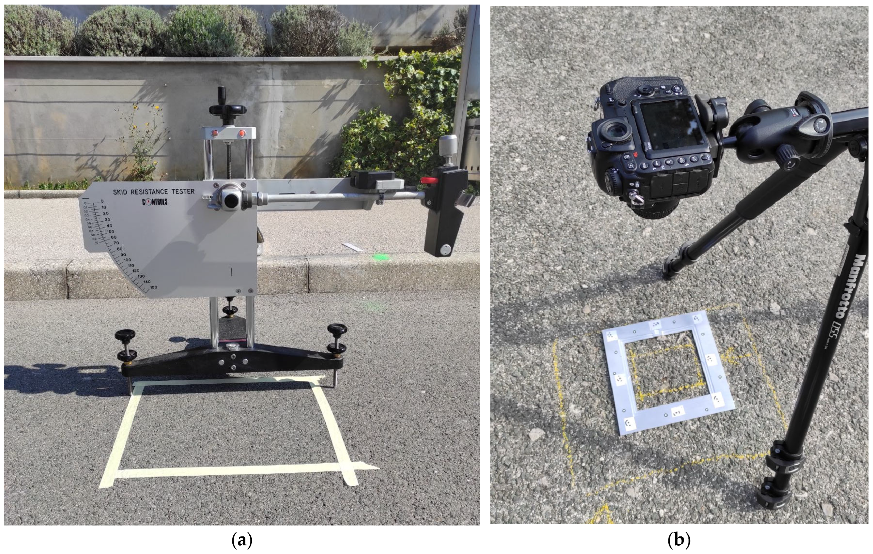
  • Application of a new experimental method named Close-Range Orthogonal Photogrammetry (CROP) for the creation of pavement surfaces database for further roughness analysis, described in Section 3.1.
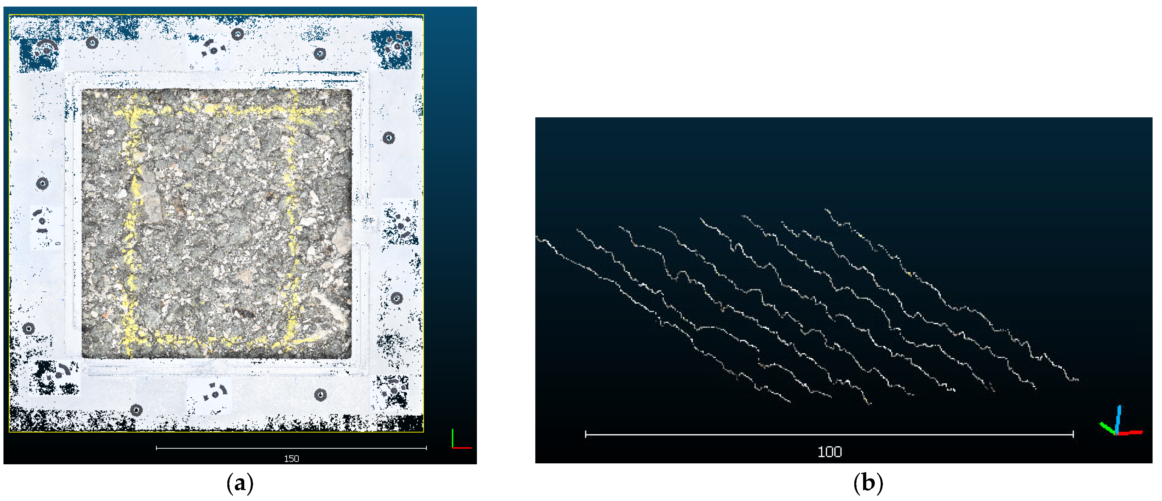
  • Creation of 3D digital surface models (DSMs) from the pavement surfaces database for the analysis of roughness features on surface profiles, detailed in Section 3.2.
  • Selection of relevant texture roughness parameters for the establishment of the skid resistance performance predictive model, elaborated in Section 3.3.
A graphical summary of performed experimental research activities is given in Figure 2. Each activity will be described more in detail in the following sections.

3.1. Pavement Surface Data Collection by the CROP Method

In pursuit for a detailed description of pavement texture morphology, first a reliable method for texture data collection and analysis was to be established. Following the results and conclusions derived from previous research utilizing optical measurement methods for texture data acquisition overviewed in previous chapter, this research aimed to investigate the applicability of existing photogrammetric equipment for the analysis of pavement texture roughness features. The photogrammetry method was used in this research as an existing expertise, applied earlier to some large-scale civil engineering problems [55,56]; therefore, the necessary equipment, i.e., a digital camera, for data acquisition were available as research resources.
Experimental procedures performed in the process of the method’s development and verification are thoroughly described in [15]. The method was named Close-Range Orthogonal Photogrammetry—the CROP method—as the pavement surface images were captured with a camera positioned orthogonally to the pavement surface from a 0.5 m height. The method was suitable for pavement texture data acquisition on full scale of macro-texture and micro-texture up to 0.01 mm in lateral and vertical directions, obtaining higher accuracy than previous research utilizing photogrammetry as data acquisition method [50]. The CROP method was verified for its accuracy and precision by performance comparison with a high-end 3D laser scanning equipment. The obtained verification results presented in [15] proved the method’s suitability for the analysis of pavement surface morphology features related to its frictional performance.
The CROP method was applied to collect the pavement texture roughness data from 20 asphalt pavement surfaces on urban road network locations. The goal was to investigate the effect of surface texture features on friction performance without including any other influencing factors, such as surface asphalt mixture type, age or traffic load. Furthermore, environmental effects on friction performance were excluded as data were collected under same weather conditions for all locations. The only known property was the friction performance measured by a static device—a pendulum—following the standard for measurement procedure expressed as skid resistance value SRT [10]. Skid resistance was measured in dry surface conditions, to eliminate the effect of water on the frictional properties of inspected surfaces. The measurement results are given in Figure 3, expressed as SRT number specific for each inspected surface, ranging from SRT = 68.4 for surface no. 3 to SRT = 103.2, determined for surface no. 17.
The procedure for texture roughness data collection followed the skid resistance measurements. The exact area of skid resistance evaluation on each inspected pavement surface was marked so the texture can be acquired on the same area and roughness features could be compared to the friction performance of the exact same surface. The size of inspected area was approximately 125 mm × 75 mm, corresponding to the surface measured by a skid resistance pendulum device [10]. Previously performed research [39] investigated optimal size of evaluation area for pavement texture roughness analysis and concluded that the minimal size of inspected area should be 80 mm × 80 mm. To assure precise image acquisition and further model reconstruction, a custom-made aluminum reference and calibration frame was placed on the marked surface. A digital camera Nikon D500 20 Mpix with AF Nikkor 50 mm f1.8D lens was used for image acquisition. Camera was mounted on a tripod with a fixed height of 0.5 m and positioned orthogonally to the surface. Images were taken consecutively to capture the surface inside the reference frame by moving the camera along the horizontal and vertical edges of the frame in a 5 × 5 grid. Each consecutive image was overlapped with the previous one for 60% side and 80% forward overlap, following the recommendations given in [57]. A total of 25 surface images were captured. Two additional images of the whole upper half and lower half of the reference frame were captured for the sake of accuracy improvement in the surface model reconstruction procedure. An example of SRT measurements and surface data acquisition by the CROP method is given in Figure 4.

3.2. Digital Surface Models (DSM) Creation

Acquired images were utilized in the process of digital surface model (DSM) creation for further analysis of surface roughness properties. This was performed in a specialized photogrammetry software Agisoft Metashape, v1.5 Pro, LLC, Sankt Petersburg, Russia. Images were acquired in RAW format to save the original data stored in a pixel, whose size was 4.31 × 4.31 microns. Afterwards, images were pre-processed and stored in 16-bit TIFF format compatible with the photogrammetry software, to avoid any data loss or distortion of originally captured images. For each inspected surface, a unique folder was created in the software where all corresponding images were imported. Each folder consisted of 27 images and a set of DSM reconstruction properties related to the alignment and reconstruction procedure. The reconstruction properties were previously determined on laboratory samples and applied to all investigated surfaces so the roughness properties analyzed in this study can be comparable. The described reconstruction procedure in the following text was applied equally to all surfaces, with detailed explanations in [15].
The reconstruction procedure in Agisoft Metashape software is based on seek-and-match procedure of common points in all acquired and imported images, used for the image alignment as a precondition for the 3D object reconstruction. The DSMs were reconstructed by setting up the same properties for image alignment and model reconstruction, generating a set of common points as a basis for the DSM reconstruction. The final set of points resulting from the seek-and-match and alignment procedures represents a sparse point cloud (SPC) entity. The SPC entity was subjected to further adjustments by three error reduction features to improve the final model’s quality: reconstruction uncertainty, projection accuracy and reprojection error. Reconstruction uncertainty reduces the model’s error by excluding the points that are generated from poor geometric relations of the camera and therefore reduces the noise and highly uncertain points. Projection accuracy feature seeks the points having low values of match accuracy generated by the seek-and-match algorithm of the software. Reprojection error is applied to sort out the points in SPC which were generated by a false match procedure, meaning that such points represent a weak estimation of a true point location after the alignment was performed. In this research, the error reduction features were selected starting from the initial values recommended by the software setup and increased gradually to remove 10% of SPC points with lowest quality. After each iteration, three SPC features were analyzed to indicate the potential improvement of the model: reprojection error value for the reconstruction uncertainty feature, Mean Key Point Size value for the projection accuracy feature and RMS reprojection error value for the reprojection error feature. The procedure of model optimization was terminated when the RMS reprojection error was equal to or below 0.3 for the lowest values of reprojection error and Mean Key Point Size. These threshold values were adopted from [57].
The SPC object established by applying the described error reduction features was the basis for the reconstruction of the digital surface model (DSM) in a form of a dense point cloud (DPC) object. The DPC is a 3D entity consisting of a large number of points with defined XYZ coordinates, describing the morphology features of inspected surfaces. For each investigated surface, the same settings were applied in the reconstruction procedure of pavement DSMs. The properties of all resulting DSMs is available as a part of research database created in [15]. An example of created DSMs and sectioned profiles is presented in Figure 5.

3.3. Texture Data Processing and Analysis—Profile-Related and Surface-Related Texture Parameters

To investigate the surface morphology properties of created DSMs, the DPC entities were further processed in an open-source software for point cloud data analysis CloudCompare, v2.11.3 (Anoia), Paris, France. The models were scaled to correspond to millimeter unit size, levelled to remove any vertical alignment of the surface resulting from the road’s geometrical properties and segmented to exclude all DSM points falling out of the reference frame’s inner edge. The final pavement surface DSMs were sectioned to profiles. Each DSM was sectioned by profiles of 100 mm length. The profile’s length was selected to correspond the length specified for the calculation of traditional pavement texture profile-related indicator, MPD [5]. The lateral distance between the profiles was selected to be 10 mm in the profile extraction procedure, to cover the whole surface measured by SRT pendulum. The lateral distance of the extracted profiles was selected arbitrary, as no recommendations were found in previous similar research. However, to investigate how the number of extracted profiles affected the mean roughness representation of analyzed surfaces, traditional roughness parameter MPD and non-standard parameters Pa, Pq, Pz and Pc described in Table 2 were calculated for all extracted profiles on a trial surface. Furthermore, mean value of these parameters were calculated separately for even and odd profiles and for the whole profile dataset. The analysis of statistical variability indicators standard deviation, variance and coefficient of variation showed no significant difference in the mean values of analyzed roughness parameters [15]. Therefore, the lateral distance of 10 mm was considered acceptable for roughness analysis on all investigated surfaces. A total of 180 profiles were sectioned from all analyzed pavement surfaces by applying the same settings in the profile extraction procedure. The number of profiles varied from eight to ten for each surface, depending on the exact width of the analyzed DSM. The number of points in each sectioned profile was slightly different, with respect to the surface morphology on a given profile’s position. Furthermore, the profile extraction procedure required the specification of profile’s section thickness, i.e., the width of the zone in the DPC entity from which the profile was extracted. A comparison of two different section thicknesses was performed on a trial surface to determine the optimal thickness [15]. The analysis showed that selected profile section thickness of 0.01 mm generates profiles with higher average horizontal resolution, which implies more detailed roughness representation capturing both micro- and macro-scale of texture. The selected optimal section thickness of 0.01 mm generated profiles with average point density of 70 pts/mm.
The calculation of profile-related roughness parameters was performed in MountainsLab, v9.3 software where sectioned surface profiles were imported and processed prior to the parameters’ calculation. The processing involved profile slope suppression and profile data filtering by a low-pass Gaussian filter with 2.5 microns set as threshold value to remove all noise-like data irrelevant for the analysis of friction-related texture morphology, with respect to the acquired CROP method’s accuracy. Selected profile-related roughness parameters were calculated on primary profiles, i.e., the profiles including both micro- and macro-texture scale, following the standard [44]. The parameters were selected in the amplitude-related group and profile features group as peak and element parameters. Traditional profile-related parameter MPD was calculated separately for all sectioned profiles, following the standard [5]. Selected texture parameters and their descriptions are given in Table 2.
The selected non-standard texture parameters were subjected to exploratory data analysis in XL Stat-Basic+, v.2022.4.5 software to determine their statistical properties, such as data distribution type and correlation strength. Profile-related non-standard parameters showed non-normal distribution. Correlation strength was evaluated by non-parametric Kendall’s correlation coefficient indicating monotonic but non-linear relationship, with threshold values of 0.4 as indicator of moderate correlation and 0.6 as indicator of strong relationship, adopted from [58,59]. The strongest correlation between non-standard parameter and traditional MPD was obtained for Ppt parameter and the weakest correlation was obtained for the MPD and Pvt parameter. Four parameters were excluded from the further analysis as they showed no statistical significance in the correlation analysis: Psk, Pku, Psm and Psmx (Table 3).
To relate texture roughness parameters to measured friction performance, profile-related parameters were converted to surface-related parameters. To do so, calculated parameters were divided in two groups: overall roughness parameters and extreme roughness parameters. The first group consisted of four non-standard parameters describing profile’s overall roughness property as they were calculated as a mean value of a profile feature for a full profile length. These parameters were Pa, Pq, Pz and Pc. Traditional parameter MPD was also categorized as an overall roughness parameter, evaluated from the mean profile features on full profile length. The extreme roughness parameters group included four parameters calculated from an extreme profile feature, profile peak or profile pit: Pt, Ppt, Pvt and Pcx. To convert profile-related parameters to their surface-related equivalents, homogeneity of profiles sectioned from a single surface was evaluated. Homogeneity was evaluated by coefficient of variation (CV) for the overall roughness profile-related parameter Pa calculated for all the profiles belonging to the same surface. If the profiles were found to be homogenous, the mean value of overall roughness parameter calculated for all profiles sectioned from the same surface was considered to be a genuine representation of surface’s roughness feature. A value of CV = 19% was set to be a threshold value for homogeneity classification. It was calculated as a 3rd quartile value for all calculated CVs of Pa parameter on all inspected surfaces. Homogeneity analysis showed that 75% of surfaces are homogenous and, therefore, the mean values of overall roughness parameters determined from profile-related parameters values could be adopted as surface-related texture roughness features. The values of extreme roughness parameters were adopted as absolute maximum values in the profile dataset belonging to the same surface. The extreme roughness parameters values were not averaged to avoid the reduction in parameters’ values that could influence the results of the future predictive model.
Surfaces classified as non-homogenous were further processed by excluding the profiles characterized as outliers, detected by a custom outlier test. For each surface, the absolute difference between mean value of Pa parameter and its absolute maximum value in a surface-related dataset was calculated. The profile having the highest absolute difference was selected as the potential outlier profile. The values of extreme roughness parameters determined for this potential outlier were compared to the absolute maximum values of extreme roughness parameters in the corresponding surface dataset. Profiles having extreme roughness parameters values lower than the determined absolute maximum values were excluded from the surface dataset and mean overall roughness parameters values were re-calculated with reduced number of profiles and compared to the defined threshold value for homogeneity. In case when the highest extreme roughness parameters values were equal to those of the potential outlier profile, they were not directly excluded from the dataset as these extreme values might affect the roughness characterization of the surface and future prediction model. If the difference between the absolute maximum and the next highest value of extreme roughness parameters was below 0.1 mm, the profile was after all selected as an outlier as this difference was considered to be insignificant for the later model development. For differences larger than 0.1 mm, the surfaces remained categorized as non-homogenous. The outlier analysis found two non-homogenous surfaces with two extreme roughness parameters having higher difference between extreme value and the next highest parameter value: Pcx and Pt. However, as the differences were slightly higher than the established threshold value, these surfaces were not excluded from the analysis but considered as non-homogenous. A special attention was given to the parameters Pcx and Pt in further analysis and establishment of the predictive model.
The final dataset included twenty sets of surface-related texture parameters, corresponding to the inspected surfaces. Each set consisted of four overall roughness parameters and four extreme roughness parameters [44] and one standard pavement texture evaluation parameter MPD [5]. This dataset was also tested for distribution type, again showing non-normal distribution of parameters. Kendall’s correlation coefficients are given in Table 4, where it can be seen that most parameters exhibit statistically significant correlation with each other and moderate to strong correlation to measured friction, except the parameter Pvt which was also statistically insignificant for the SRT values. Correlation analysis was performed to investigate the relationship among the parameters and their correlation to measured friction performance expressed in SRT values. Kendall’s correlation coefficient was again selected as a measure of monotonic and non-linear relationship, since the generated scatter plots showed no strong linear relationship (Figure 6). Obtained coefficients of determination range from 0.146 for Pvt to 0.587 for Ppt parameter versus SRT friction.
Traditional pavement texture parameter MPD showed a significant correlation to several non-standard texture parameters, especially Ppt, Pz and Pc. A meaningful correlation was obtained between MPD and measured SRT values and generated scatter plot showed a positive and monotonic moderate linear relationship with coefficient of determination of 0.592 (Figure 7). This linear regression model with MPD as the only predictor was statistically significant with model error metric value RMSE = 6.162.
The newly proposed experimentally derived method for pavement texture data acquisition—the CROP method—was suitable for roughness analysis on micro- and macro-scale of texture with obtained resolution of 0.01 mm in all directions and accuracy of up to 0.05 mm, verified by a benchmark optical measurement method 3D high-precision laser scanner [15]. The stablished CROP method’s performance enabled the roughness analysis of investigated surfaces on full macro-texture scale and micro-texture scale up to 0.01 mm. The CROP method for texture data assessment enables a more detailed description of roughness features in comparison to traditional texture characterization methods, which is the main advantage of the proposed method. Previous research results showed that traditional texture parameters obtained by similar photogrammetry-based methods are comparable to the same indicators obtained by traditional measurement techniques [49,53]. This makes the photogrammetry-based techniques a potential substitute for traditional measurement methods, with more detailed and accurate characterization of roughness features. Therefore, obtained roughness parameters were further analyzed to investigate if they could provide more reliable relationship to the measured friction performance.

4. Friction Prediction Model Development

Following the results of performed exploratory data analysis of the texture dataset, four non-standard parameters were selected for further predictive model development: Pa, Pz and Pc as overall roughness parameters and Ppt as an extreme roughness parameter. They obtained the highest correlation coefficients with measured SRT values and moderate positive linear relationship, given in scatter plots in Figure 6. The first attempt to develop a friction performance prediction model by using significant non-standard texture parameters as model predictors was performed by using all four parameters for model establishment in the multiple linear regression (MLR) framework. The initial MLR model consisted of four predictors and resulted in better model performance in comparison to the simple friction prediction model using only MPD parameter as a predictor (Table 4). However, analysis of variance and sum of squares analysis indicated that the parameter Pa is not statistically significant for the model and it was excluded in the next model iteration. The second model version observed three predictors, where again one of them (Ppt) was statistically insignificant. Another issue was the negative sign of coefficient attributed to the Pc, which was contrary to the previous correlation analysis results showing a positive monotonic relationship with all texture parameters and friction. The final prediction model involved two non-standard parameters, Pz and Pc, with coefficient of determination R2 = 0.720 and RMSE of 4.970 which again, in comparison to the initial simple model showed better predictive strength (Table 5). However, the model’s reliability was violated due to the multicollinearity issue between the predictors detected by variance inflation factor (VIF) value exceeding recommended threshold value of VIF < 10 for no collinear variables [60]. If there exist multicollinearity between the predictors, the model’s strength and confidence could be jeopardized. Some examples given in [60,61] are wrong coefficient signs due to the mixed effect of predictors to regression coefficients, model instability evident in a notable change in regression coefficient for a slight change in model input, increase in standard error estimate and test insignificance or confidence intervals widening. Therefore, it was necessary to solve the multicollinearity problem to deliver a reliable prediction model in the MLR framework.
The simplest method for multicollinearity removal is to reject highly collinear and insignificant predictors from the model [61]. This approach is particularly useful in case when there is a large number of model predictors having various influences to the model and resulting from different data sources. This solution was not applicable in this study as all four texture parameters were significant for the friction performance. Also, they all described a specific roughness feature of texture morphology and none of them was to be excluded “a priori”. The second approach would be to implement some feature engineering procedures to the existing dataset, such as regularization techniques or dimensionality reduction techniques [62,63]. In this way, none of the original predictors is directly excluded from the model and categorized as insignificant. In regularization techniques predictors are modified by penalization of “original” model coefficients to reduce their variance, while in the dimensionality reduction techniques the predictors are combined to composite variables whose number is usually smaller than the number of “original” predictors. To investigate the effect of feature engineering techniques, the initial MLR model was subjected to ridge regression regularization, principal component regression and partial least squares regression.

4.1. Model Development by Ridge Regression Regularization

Ridge regression is a regularization method for model generalization by a penalty term added to the loss function, with the aim to reduce the variance of the model’s coefficients [61]. The penalty term l is introduced in the loss function RSS (residual sum of squares) through a squared coefficient value b [61],
R S S = i = 1 n ( Y i j = 1 p X i j β j ) 2 + l j = 1 p β j 2
where Yi is the actual response variable and Xijβj is the predicted value of response variable calculated from predictors Xij and coefficients βj. The magnitude of the penalty term regularizes the variance reduction; therefore, it is important to adequately select the proper value of l. In case when the value is too small (close to zero), there is no effect to the loss function and ridge regression would converge to simple MLR. On the other hand, if l is too large it could cause model under-fitting [62]. To avoid manual tuning of penalty parameter, a k-fold cross-validation method was applied to select the optimal value of l with k = 5 and k = 10 folds, resulting in two different penalty terms used for the model establishment. Both models were defined with all four predictors (Pa, Pz, Pc and Ppt), with resulting model statistics shown in Table 5. The model showed better performance for penalty obtained by 5-fold cross-validation; therefore, it was further optimized. A Z-score outlier test was performed to exclude potential outliers from the dataset, resulting in an enhanced model version. By observing the coefficients associated to the predictors, two of them were negative which was contrary to the initial correlation analysis, where all texture parameters showed a positive monotonic relationship with friction. The “negative” parameters were excluded in the next iteration step and the final prediction model was defined by two predictors, Pz and Ppt. The model statistics obtained for the final model version (V2) were improved in comparison to the previous iterations (Table 6).

4.2. Model Development by Principal Components Regression

Principal components analysis (PCA) is a dimensionality reduction technique for resolving the multicollinearity problem in prediction models [64]. The key feature of this feature engineering technique is to create new model variables as a linear combination of original variables, called principal components [65]. These new variables are orthogonal so they are no longer collinear; therefore, the multicollinearity issue is resolved [66]. The number of resulting principal components k is usually lower than the number of original model predictors n, so the problem dimension is reduced. The selection of principal components is based on their eigen values, resulting from spectral decomposition of original predictors matrix. If the eigen value of a given principal component is equal or higher than 1, it is considered as a significant predictor for the model. Also, if the principal component’s eigen value describes dominantly the data variance (usually 90% or more), it is considered to be a significant new model predictor [64].
The results of performed PCA for the selected non-standard texture parameters dataset is given in Table 7. From the calculated eigen values, it can be seen that only the first principal component PC1 obtained value higher than 1. By observing the contribution of each principal component to the variance, in addition to the PC1, there is a significant contribution of PC2 to the variability for the parameter Ppt. Therefore, two versions of prediction models were evaluated: one with only one principal component PC1 and another with two principal components, PC1 and PC2.
Prediction models were defined with principal components PC1 and PC2, consisting of original predictors attributed with calculated factor loadings as coefficients,
P C 1 = 0.986 P a + 0.987 P z + 0.985 P c + 0.905 P p t
P C 2 = 0.116 P a 0.117 P z 0.157 P c + 0.424 P p t
New model predictors were no longer collinear; however, some of the coefficients showed a negative sign. Therefore, another model iteration was tested with only one principal component PC1 as a predictor. Model was tested for outliers with Z-score test, showing one critical value which was excluded from the dataset. The final PCA regression model iteration showed no outliers and all the coefficients associated to the original model predictors were positive (Table 8).

4.3. Model Development by Partial Least Squares Regression

Another dimensionality reduction technique applied in this study was the partial least squares (PLS) method. Similar to the PCA method, in the PLS method the dimensionality of the observed problem is reduced by creating new composite variables whose number is usually lower than the number of original variables [62]. The difference between PCA and PLS is that the PLS method accounts not only for the predictors but also the model output in the process of new variables creation. The goal of this method is to find the linear combination of predictors’ associated coefficients which would result in a maximization of covariance between the predictors and model output [67]. PLS is considered as more efficient when the research goal is to define a prediction model in the MLR framework, in comparison to PCA [64]. The new model predictors resulting from the PLS method are called latent variables (LVs), whose coefficients are iteratively calculated to obtain the maximum covariance between the predictors and model output [68]. The coefficients’ weights indicate the importance of original predictors to the new latent variables and their contribution to the model output. In the PLS method, the values of variable importance in the projection or VIP scores are evaluated for all original predictors. These values are an indicator of predictors’ importance in the definition of PLS components (LVs), where a VIP score > 1 marks a highly important variable and a VIP score < 0.8 marks a predictor with no significant influence to the component’s definition [68].
PLS regression was defined with one latent variable created as a linear combination of all four non-standard texture parameters and measured friction values. The initial PLS prediction model’s performance was weaker in comparison to the initial LR model; therefore, the model was optimized by excluding the outlier data detected by Z-score test and by selecting only the predictors with VIP score > 1. In this way, the performance of the final PLS regression model was improved, as can be seen from Table 9.

4.4. Comparison of Predicition Models’ Performance

The proposed friction predictive models were defined in XL Stat-Basic+, v.2022.4.5 software by application of built-in feature engineering procedures for ridge regression, PCA regression and PLS regression. The final versions of all three models and the resulting model performance statistics R2 and RMSE are compared in Table 10. Model performance was evaluated on the validation dataset, selected randomly from the full dataset by following the 75/25 rule for training and validation data. The results show that the best performance is obtained for the PLS regression model, having highest coefficient of determination R2 and lowest value of RMSE. The PCA regression model showed the weakest performance, while the ridge regression model with two predictors showed similar performance to the PLS regression model.
Figure 8 presents the regression plots for the training and validation dataset obtained for all three proposed models. In comparison to the initial LR predictive model where only the traditional MPD texture parameter was used as the model predictor, all three proposed models showed better predictive strength.
The success of the PLS regression model’s performance could be attributed to the method’s algorithm, which accounts for linear relationship not only among model predictors, but also between the predictors and model output in the creation of latent variables. Another advantage of the PLS regression model is the calculation of variable importance in projection (VIP) scores based on obtained latent variables, which provides automatic selection of the most significant predictors in the model. None of the coefficients associated to the model predictors in the PLS regression model was negative in any of the model’s iterations; therefore, it can be concluded that PLS-generated model parameters are the closest to the actual positive and monotonic relationship between texture roughness features and pavement friction, explored in the initial correlation analysis. The selection of texture parameters as model predictors based on their VIP scores optimized the model’s performance and showed that the predictive strength does not depend on the number of predictors but on their effect to the model outcome.

5. Discussion

In this study, the originally developed method named Close-Range Orthogonal Photogrammetry (CROP) was used for pavement texture data collection and analysis. The CROP method is based on photogrammetry technology as an alternative method for texture roughness characterization, recently in use for a thorough investigation of relationship between pavement texture morphology and friction performance. The method enables simple texture data collection by using a single digital camera for surface images acquisition, from which digital surface models are created and further analyzed. A detailed description of the method’s development and verification is given in [15].
The CROP method was applied for texture data collection and analysis on twenty selected asphalt pavement surfaces of various road sections, where low-speed friction performance was previously determined. The method was suitable for pavement texture data acquisition on full scale of macro-texture and micro-texture up to 0.01 mm. The accuracy of experimentally derived method was verified by performance comparison of digital surface models created by the CROP method and the benchmark method for optical measurements—a high precision 3D laser scanning device, with obtained deviations of measured dimensions up to 0.05 mm. In some previous research where a new photogrammetry-based method was proposed for texture data acquisition [37,69], the validation procedure was performed with traditional texture parameters MPD or MTD, determined traditionally. In this way, the proposed method’s precision in terms of actual geometry of roughness features or the accuracy of calculated roughness parameters other than the traditional ones could not be determined, as in the case for the CROP method.
Texture roughness parameters were analyzed on digital surface model profiles, extracted from each investigated surface equally by following the established data analysis procedure. Selected non-standard texture parameters and the traditional texture parameter MPD were calculated for all extracted profiles, without the scale separation to micro- and macro-texture levels, following the conclusions of previous research [48]. In comparison to similar research utilizing photogrammetry technique for texture roughness data acquisition, where texture parameters were calculated separately for micro- and macro-scale [50,70], the results obtained in this study showed that scale separation should not be performed prior to the investigation of texture–friction relationship.
The predictive model was developed in the multiple linear regression framework, which is a simple method for model establishment and interpretation, especially in case when the dataset has a limited size [62]. The overviewed empirical predictive models are mostly established within the LR framework, accounting for one or more parameters related to the pavement’s frictional performance. As pavement texture is one of significant friction influencing parameters related to the properties of pavement materials, it was selected as the exclusive parameter in the model. The performance of initial friction model accounting only MPD parameter calculated from pavement DSMs was comparable to models developed in similar research by [71,72]. The obtained simple LR model’s performance was moderate, with R2 equal to 0.592; therefore, additional non-standard texture roughness features were included as predictors in the proposed models. Friction predictive models were defined by three different feature engineering procedures, which was a novel approach for the development of a friction performance prediction model in the linear regression framework. This was performed as the predictors were collinear and none of them was considered as less significant to be excluded a priori from the dataset. The applied procedures were ridge regularization, principal components analysis (PCA) and partial least squares (PLS) analysis. In comparison to the initial LR model, all three procedures resulted in a final model with better performance. The predictive strength of proposed models was evaluated by the resulting coefficient of determination R2 and error metric RMSE. In case of the ridge regularization regression model the obtained R2 was 0.767 and RMSE 4.442, for the PCA regression model R2 was 0.667 and RMSE 5.757 and for the PLS regression model the R2 was 0.780 and RMSE 4.412. The presented results were obtained for the validation dataset, selected randomly from the whole dataset by following 75/25 rule. The final model was defined within the partial least squares (PLS) regression algorithm, showing the best model performance values. Furthermore, the PLS regression model selected the most significant texture parameters with the highest influence on friction performance evaluated through VIP scores of predictors: amplitude parameter maximum height Pz and feature parameter maximum peak profile height, Ppt. The former describes an overall roughness property and the latter is a description of extreme surface roughness. The final PLS regression model showed superior performance in comparison to similar research where photogrammetry-based method was used for texture data assessment in friction prediction model establishment [48,69,73].
The error metric RMSE was selected as one of the predictive model’s performance measures. The final model’s performance for the obtained RMSE for the validation dataset was 4.412 (Table 9), which is not a negligible difference in friction performance assessment by a static pendulum measurement device. This indicates the necessity of further improvements of the proposed predictive model in the PLS regression framework for a more accurate prediction of measured friction values. As a limitation of the performed study a relatively small dataset and a narrow range of measured SRT values can be pointed out. A larger dataset with a broader range of measured SRT values, including low-level friction surfaces which were not included in this study, could contribute to the improvement of the model’s performance.

6. Conclusions

The aim of this study was to establish a pavement friction predictive model with texture roughness features as exclusive model predictors. For this purpose, pavement surfaces were analyzed by a novel, originally developed method for 3D texture data collection. The method was named Close-Range Orthogonal Photogrammetry (CROP) method and it was experimentally developed and verified as a part of author’s doctoral thesis research. The CROP method was utilized for collection of pavement surface images, used as input for 3D digital surface model creation. Texture roughness parameters were calculated from the profiles extracted from the DSMs and used for the establishment of the friction predictive model in the partial least squares (PLS) regression framework.
The main conclusions drawn from this research are:
  • The developed photogrammetry-based CROP method is applicable for pavement texture roughness characterization in micro- and macro-texture scale, resulting in digital surface models with sub-millimeter resolution. This makes the CROP method suitable for analysis of texture morphology on full scale of macro-texture and micro-texture up to 0.01 mm, with accuracy of 0.05 mm confirmed by a benchmark 3D data acquisition method with a high-end laser scanning device.
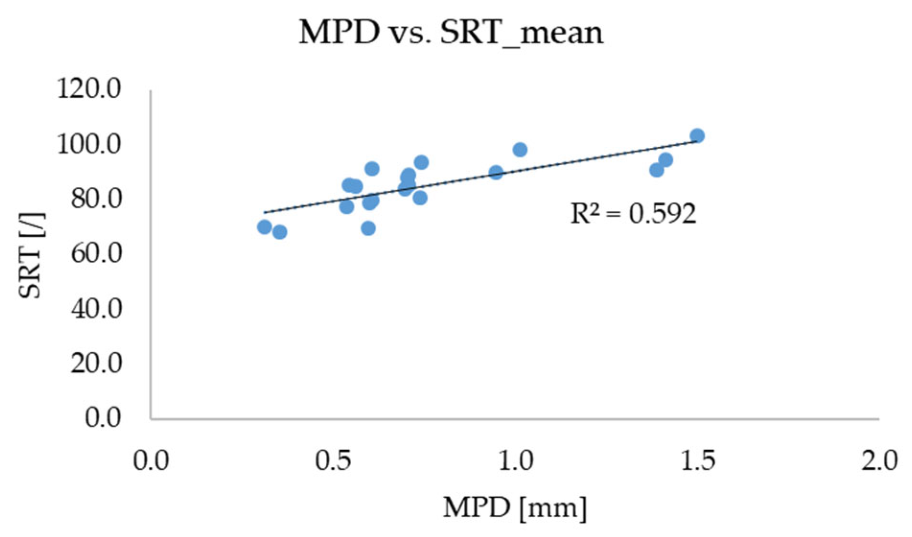
  • Traditional texture characterization parameter MPD derived from digital surface models showed a notable correlation to measured friction, proving that digital surface models are realistically representing the actual surface roughness characteristics.
  • Non-standard texture roughness parameters obtained from digital surface models are suitable predictors in the establishment of pavement texture–friction relationship. Analysis showed that the amplitude and feature parameters with the most significant impact on friction performance are maximum height Pz, describing overall roughness property and maximum peak profile height, Ppt, describing extreme roughness property of a pavement surface.
  • The proposed predictive model’s performance was superior in comparison to that of the initial model defined by a single traditional texture indicator Mean Profile Depth (MPD), showing that non-standard texture parameters better describe the effect of texture roughness on frictional characteristics of a pavement surface. The obtained R2 of the proposed PLS regression model was 0.780 while the predictive model with the traditional MPD indicator obtained R2 of 0.592.
By comparing predictive models proposed in previous similar studies where optical method utilizing digital camera was used for texture data assessment, the PLS regression model showed better performance. Further model improvements will be made by extending the database size and range of measured friction values. True surface-related texture parameters in the 3D framework will be calculated from the digital surface models and used as predictors for the model’s performance improvements. Further analyses of asphalt mixture type properties in terms of roughness features related to frictional response will be conducted in the next research phase.

Author Contributions

Conceptualization, I.B., A.D.-T. and I.R.; methodology, I.B.; software, I.B.; validation, I.B.; formal analysis, I.B.; investigation, I.B.; data curation, I.B.; writing—original draft preparation, I.B.; writing—review and editing, A.D.-T. and I.R.; visualization, I.B.; supervision, A.D.-T. and I.R. All authors have read and agreed to the published version of the manuscript.

Funding

This research received no external funding.

Data Availability Statement

The dataset presented in this study is a part of research database created in a doctoral thesis research and is available upon request from the corresponding author.

Acknowledgments

This research is supported by the University of Rijeka scientific project Transport infrastructure in the function of sustainable mobility.

Conflicts of Interest

The authors declare no conflict of interest.

References

  1. Fwa, T.F. Determination and prediction of pavement skid resistance–connecting research and practice. J. Road Eng. 2021, 1, 43–62. [Google Scholar] [CrossRef]
  2. Persson, B.N.J. Theory of rubber friction and contact mechanics. J. Chem. Phys. 2001, 115, 3840–3861. [Google Scholar] [CrossRef]
  3. Persson, B.N.J.; Albohr, O.; Tartaglino, U.; Volokitin, A.I.; Tosatti, E. On the nature of surface roughness with application to contact mechanics, sealing, rubber friction and adhesion. J. Phys. Condens. Matter 2005, 17, R1. [Google Scholar] [CrossRef]
  4. Heinrich, G.; Klüppel, M. Rubber friction, tread deformation and tire traction. Wear 2008, 265, 1052–1060. [Google Scholar] [CrossRef]
  5. EN ISO 13473-1; Characterization of Pavement Texture by Use of Surface Profiles—Part 1: Determination of Mean Profile Depth. HZN: Zagreb, Croatia, 2004.
  6. Hall, J.W.; Smith, K.L.; Titus-Glover, L.; Wambold, J.C.; Yager, T.J.; Rado, Z. Guide for Pavement Friction; National Cooperative Highway Research Program; The National Academies Press: Washington, DC, USA, 2009. [Google Scholar] [CrossRef]
  7. Kogbara, R.B.; Masad, E.A.; Kassem, E.; Scarpas, A.; Anupam, K. A state-of-the-art review of parameters influencing measurement and modeling of skid resistance of asphalt pavements. In Construction and Building Materials; Elsevier Ltd.: Amsterdam, The Netherlands, 2016; Volume 114, pp. 602–617. [Google Scholar] [CrossRef]
  8. EN 13036-1; Road and Airfield Surface Characteristics—Test Methods—Part 1: Measurement of Pavement Surface Macrotexture Depth Using a Volumetric Patch Technique. HZN: Zagreb, Croatia, 2011.
  9. Li, Q.; Yang, G.; Wang KC, P.; Zhan, Y.; Wang, C. Novel Macro- and Microtexture Indicators for Pavement Friction by Using High-Resolution Three-Dimensional Surface Data. Transp. Res. Rec. 2017, 2641, 164–176. [Google Scholar] [CrossRef]
  10. EN 13036-4; Road and Airfield Surface Characteristics—Test Methods—Part 4: Method for Measurement of Slip/Skid Resistance of a Surface: The Pendulum Test. HZN: Zagreb, Croatia, 2012.
  11. EN 13036-2; Road and Airfield Surface Characteristics—Test Methods—Part 2: Assessment of the Skid Resistance of a Road Pavement Surface by the Use of Dynamic Measuring Systems. HZN: Zagreb, Croatia, 2011.
  12. Andriejauskas, T.; Vorobjovas, V.; Mielonas, V. Evaluation of skid resistance characteristics and measurement methods. In Proceedings of the 9th International Conference on Environmental Engineering, ICEE 2014, Pune, India, 21–23 February 2014. [Google Scholar] [CrossRef]
  13. Rajaei, S.; Chatti, K.; Dargazany, R. A review: Pavement Surface Micro-texture and its contribution to Surface Friction. In Proceedings of the Transportation Research Board 96th Annual Meeting, Washington DC, USA, 8–12 January 2017; p. 17-06773. [Google Scholar]
  14. Yu, M.; You, Z.; Wu, G.; Kong, L.; Liu, C.; Gao, J. Measurement and modeling of skid resistance of asphalt pavement: A review. In Construction and Building Materials; Elsevier Ltd.: Amsterdam, The Netherlands, 2020; Volume 260. [Google Scholar] [CrossRef]
  15. Ban, I. A Model for Skid Resistance Prediction Based on Non-Standard Pavement Surface Texture Parameters. Ph.D. Thesis, University of Rijeka Faculty of Civil Engineering, Rijeka, Croatia, 2023. [Google Scholar]
  16. Rezaei, A.; Masad, E. Experimental-based model for predicting the skid resistance of asphalt pavements. Int. J. Pavement Eng. 2013, 14, 24–35. [Google Scholar] [CrossRef]
  17. Sansoni, G.; Trebeschi, M.; Docchio, F. State-of-the-art and applications of 3D imaging sensors in industry, cultural heritage, medicine, and criminal investigation. Sensors 2009, 9, 568–601. [Google Scholar] [CrossRef] [PubMed]
  18. Tang, T.; Anupam, K.; Kasbergen, C.; Kogbara, R.; Scarpas, A.; Masad, E. Finite Element Studies of Skid Resistance under Hot Weather Condition. Transp. Res. Rec. 2018, 2672, 382–394. [Google Scholar] [CrossRef]
  19. Liu, X.; Cao, Q.; Wang, H.; Chen, J.; Huang, X. Evaluation of Vehicle Braking Performance on Wet Pavement Surface using an Integrated Tire-Vehicle Modeling Approach. Transp. Res. Rec. 2019, 2673, 295–307. [Google Scholar] [CrossRef]
  20. Peng, Y.; Li, J.Q.; Zhan, Y.; Wang, K.C.; Yang, G. Finite Element Method-Based Skid Resistance Simulation Using In-Situ 3D Pavement Surface Texture and Friction Data. Materials 2019, 12, 3821. [Google Scholar] [CrossRef]
  21. Dell’Acqua, G.; De Luca, M.; Lamberti, R. Indirect skid resistance measurement for porous asphalt pavement management. Transp. Res. Rec. 2011, 2205, 147–154. [Google Scholar] [CrossRef]
  22. Kargah-Ostadi, N.; Howard, A. Monitoring Pavement Surface Macrotexture and Friction: Case Study. Transp. Res. Rec. 2015, 2525, 111–117. [Google Scholar] [CrossRef]
  23. Kouchaki, S.; Roshani, H.; Prozzi, J.A.; Garcia, N.Z.; Hernandez, J.B. Field Investigation of Relationship between Pavement Surface Texture and Friction. Transp. Res. Rec. 2018, 2672, 395–407. [Google Scholar] [CrossRef]
  24. Islam, S.; Hossain, M.; Miller, R. Evaluation of pavement surface texture at the network level. Nondestruct. Test. Eval. 2019, 34, 87–98. [Google Scholar] [CrossRef]
  25. Li, Q.J.; Zhan, Y.; Yang, G.; Wang, K.C.P. Pavement skid resistance as a function of pavement surface and aggregate texture properties. Int. J. Pavement Eng. 2020, 21, 1159–1169. [Google Scholar] [CrossRef]
  26. Chou, C.P.; Lee, C.C.; Chen, A.C.; Wu, C.Y. Using a constructive pavement texture index for skid resistance screening. Int. J. Pavement Res. Technol. 2017, 10, 360–368. [Google Scholar] [CrossRef]
  27. Yang, G.; Li, Q.J.; Zhan, Y.J.; Wang KC, P.; Wang, C. Wavelet based macrotexture analysis for pavement friction prediction. KSCE J. Civ. Eng. 2018, 22, 117–124. [Google Scholar] [CrossRef]
  28. Pranjić, I.; Deluka-Tibljaš, A.; Cuculić, M.; Šurdonja, S. Influence of pavement surface macrotexture on pavement skid resistance. Transp. Res. Procedia 2020, 45, 747–754. [Google Scholar] [CrossRef]
  29. Ergun, M.; Iyinam, S.; Iyinam, A.F. Prediction of road surface friction coefficient using only macro- and microtexture measurements. J. Transp. Eng. 2005, 131, 311–319. [Google Scholar] [CrossRef]
  30. Ahammed, M.A.; Tighe, S.L. Asphalt pavements surface texture and skid resistance—Exploring the reality. Can. J. Civ. Eng. 2012, 39, 1–9. [Google Scholar] [CrossRef]
  31. Kotek, P.; Kováč, M. Comparison of valuation of skid resistance of pavements by two device with standard methods. Procedia Eng. 2015, 111, 436–443. [Google Scholar] [CrossRef]
  32. Meegoda, J.N.; Gao, S. Evaluation of pavement skid resistance using high speed texture measurement. J. Traffic Transp. Eng. 2015, 2, 382–390. [Google Scholar] [CrossRef]
  33. Pomoni, M.; Plati, C.; Loizos, A.; Yannis, G. Investigation of pavement skid resistance and macrotexture on a long-term basis. Int. J. Pavement Eng. 2022, 23, 1060–1069. [Google Scholar] [CrossRef]
  34. Bitelli, G.; Simone, A.; Girardi, F.; Lantieri, C. Laser scanning on road pavements: A new approach for characterizing surface texture. Sensors 2012, 12, 9110–9128. [Google Scholar] [CrossRef] [PubMed]
  35. Luhmann, T.; Robson, S.; Kyle, S.; Harley, I. Close Range Photogrammetry. 2006. Available online: https://www.researchgate.net/publication/237045019_Close_Range_Photogrammetry_Principles_Techniques_and_Applications (accessed on 5 April 2023).
  36. Puzzo, L.; Loprencipe, G.; Tozzo, C.; D’Andrea, A. Three-dimensional survey method of pavement texture using photographic equipment. Meas. J. Int. Meas. Confed. 2017, 111, 146–157. [Google Scholar] [CrossRef]
  37. Tian, X.; Xu, Y.; Wei, F.; Gungor, O.; Li, Z.; Wang, C.; Li, S.; Shan, J. Pavement macrotexture determination using multi-view smartphone images. Photogramm. Eng. Remote Sens. 2020, 86, 643–651. [Google Scholar] [CrossRef]
  38. Mathavan, S.; Kamal, K.; Rahman, M. A Review of Three-Dimensional Imaging Technologies for Pavement Distress Detection and Measurements. IEEE Trans. Intell. Transp. Syst. 2015, 16, 2353–2362. [Google Scholar] [CrossRef]
  39. Chen, S.; Liu, X.; Luo, H.; Yu, J.; Chen, F.; Zhang, Y.; Ma, T.; Huang, X. A state-of-the-art review of asphalt pavement surface texture and its measurement techniques. J. Road Eng. 2022, 2, 156–180. [Google Scholar] [CrossRef]
  40. Sha, A.; Yun, D.; Hu, L.; Tang, C. Influence of sampling interval and evaluation area on the three-dimensional pavement parameters. Road Mater. Pavement Des. 2021, 22, 1964–1985. [Google Scholar] [CrossRef]
  41. Song, W. Correlation between morphology parameters and skid resistance of asphalt pavement. Transp. Saf. Environ. 2022, 4, tdac002. [Google Scholar] [CrossRef]
  42. Zou, Y.; Yang, G.; Huang, W.; Lu, Y.; Qiu, Y.; Wang, K.C.P. Study of pavement micro-and macro-texture evolution due to traffic polishing using 3d areal parameters. Materials 2021, 14, 5769. [Google Scholar] [CrossRef]
  43. Gonzalez-Jorge, H.; Solla, M.; Armesto, J.; Arias, P. Novel method to determine laser scanner accuracy for applications in civil engineering. Opt. Appl. 2012, 42, 43–53. [Google Scholar] [CrossRef]
  44. EN ISO 21920-2; Geometrical Product Specifications (GPS)—Surface Texture: Profile—Part 2: Terms, Definitions and Surface Texture Parameters. HZN: Zagreb, Croatia, 2022.
  45. EN ISO 25178-2; Geometrical Product Specifications (GPS)—Surface Texture: Areal—Part 2: Terms, Definitions and Surface Texture Parameters. HZN: Zagreb, Croatia, 2014.
  46. Zuniga-Garcia, N.; Prozzi, J.A. High-Definition Field Texture Measurements for Predicting Pavement Friction. Transp. Res. Rec. 2019, 2673, 246–260. [Google Scholar] [CrossRef]
  47. Callai, S.C.; De Rose, M.; Tataranni, P.; Makoundou, C.; Sangiorgi, C.; Vaiana, R. Microsurfacing Pavement Solutions with Alternative Aggregates and Binders: A Full Surface Texture Characterization. Coatings 2022, 12, 1905. [Google Scholar] [CrossRef]
  48. Kogbara, R.B.; Masad, E.A.; Woodward, D.; Millar, P. Relating surface texture parameters from close range photogrammetry to Grip-Tester pavement friction measurements. Constr. Build. Mater. 2018, 166, 227–240. [Google Scholar] [CrossRef]
  49. Alhasan, A.; Smadi, O.; Bou-Saab, G.; Hernandez, N.; Cochran, E. Pavement Friction Modeling using Texture Measurements and Pendulum Skid Tester. Transp. Res. Rec. 2018, 2672, 440–451. [Google Scholar] [CrossRef]
  50. Huyan, J.; Li, W.; Tighe, S.; Sun, Z.; Sun, H. Quantitative Analysis of Macrotexture of Asphalt Concrete Pavement Surface Based on 3D Data. Transp. Res. Rec. 2020, 2674, 732–744. [Google Scholar] [CrossRef]
  51. Li, L.; Wang, K.C.P.; Li, Q.J. Geometric texture indicators for safety on AC pavements with 1 mm 3D laser texture data. Int. J. Pavement Res. Technol. 2016, 9, 49–62. [Google Scholar] [CrossRef]
  52. Hu, L.; Yun, D.; Liu, Z.; Du, S.; Zhang, Z.; Bao, Y. Effect of three-dimensional macrotexture characteristics on dynamic frictional coefficient of asphalt pavement surface. Constr. Build. Mater. 2016, 126, 720–729. [Google Scholar] [CrossRef]
  53. Chen, D. Evaluating asphalt pavement surface texture using 3D digital imaging. Int. J. Pavement Eng. 2020, 21, 416–427. [Google Scholar] [CrossRef]
  54. Kováč, M.; Brna, M.; Decký, M. Pavement Friction Prediction Using 3D Texture Parameters. Coatings 2021, 11, 1180. [Google Scholar] [CrossRef]
  55. Tadić, A.; Ružić, I.; Krvavica, N.; Ilić, S. Post-Nourishment Changes of an Artificial Gravel Pocket Beach Using UAV Imagery. J. Mar. Sci. Eng. 2022, 10, 358. [Google Scholar] [CrossRef]
  56. Ružić, I.; Marović, I.; Benac, Č.; Ilić, S. Coastal cliff geometry derived from structure-from-motion photogrammetry at Stara Baška, Krk Island, Croatia. Geo-Mar. Lett. 2014, 34, 555–565. [Google Scholar] [CrossRef]
  57. Over, J.S.; Ritchie, A.C.; Kranenburg, C.J.; Brown, J.A.; Buscombe, D.; Noble, T.; Sherwood, C.R.; Warrick, J.; Wernette, P. Processing Coastal Imagery with Agisoft Metashape Professional Edition, Version 1.6—Structure from Motion Workflow Documentation; U.S. Geological Survey: Reston, VA, USA, 2021.
  58. Akoglu, H. User’s guide to correlation coefficients. Turk. J. Emerg. Med. 2018, 18, 91–93. [Google Scholar] [CrossRef]
  59. Fredricks, G.; Nelsen, R.B. On the relationship between Spearman’s rho and Kendall’s tau for pairs of continuous random variables. J. Stat. Plan. Inference 2007, 137, 2143–2150. [Google Scholar] [CrossRef]
  60. Yoo, W.; Mayberry, R.; Bae, S.; Singh, K.; Lillard, J.W. A Study of Effects of MultiCollinearity in the Multivariable Analysis. Int. J. Appl. Sci. Technol. 2014, 4, 9. [Google Scholar] [PubMed]
  61. Schreiber-Gregory, D.N. Ridge Regression and multicollinearity: An in-depth review. Model Assist. Stat. Appl. 2018, 13, 359–365. [Google Scholar] [CrossRef]
  62. Hastie, T.; Tibshirani, R.; Friedman, J. The Elements of Statistical Learning, 2nd ed.; Springer: Berlin/Heidelberg, Germany, 2009; Available online: https://hastie.su.domains/Papers/ESLII.pdf (accessed on 15 March 2023).
  63. James, G.; Witten, D.; Hastie, T.; Tibshirani, R. An Introduction to Statistical Learning with Applications in R, 2nd ed.; Springer: Berlin/Heidelberg, Germany, 2021. [Google Scholar]
  64. Maitra, S.; Yan, J. Principle Component Analysis and Partial Least Squares—Two Dimension Reduction Techniques for Regression. 2008. Available online: https://www.semanticscholar.org/paper/Principle-Component-Analysis-and-Partial-Least-Two-Maitra-Yan/8276a0c6d57335a18547776fcfa7be639c13b822#cited-papers (accessed on 10 April 2023).
  65. Gwelo, A.S. Principal components to overcome multicollinearity problem. Oradea J. Bus. Econ. 2019, 4, 79–91. [Google Scholar] [CrossRef]
  66. Joshi, K.; Patil, B. Prediction of Surface Roughness by Machine Vision using Principal Components based Regression Analysis. Procedia Comput. Sci. 2020, 167, 382–391. [Google Scholar] [CrossRef]
  67. Liu, C.; Zhang, X.; Nguyen, T.T.; Liu, J.; Wu, T.; Lee, E.; Tu, X.M. Partial least squares regression and principal component analysis: Similarity and differences between two popular variable reduction approaches. Gen. Psychiatry 2022, 35, e100662. [Google Scholar] [CrossRef]
  68. Tran, T.N.; Afanador, N.L.; Buydens LM, C.; Blanchet, L. Interpretation of variable importance in Partial Least Squares with Significance Multivariate Correlation (sMC). Chemom. Intell. Lab. Syst. 2014, 138, 153–160. [Google Scholar] [CrossRef]
  69. Chen, J.; Huang, X.; Zheng, B.; Zhao, R.; Liu, X.; Cao, Q.; Zhu, S. Real-time identification system of asphalt pavement texture based on the close-range photogrammetry. Constr. Build. Mater. 2019, 226, 910–919. [Google Scholar] [CrossRef]
  70. Medeiros, M.; Babadopulos, L.; Maia, R.; Castelo Branco, V. 3D pavement macrotexture Parameters from close range photogrammetry. Int. J. Pavement Eng. 2023, 24, 2020784. [Google Scholar] [CrossRef]
  71. Čelko, J.; Kováč, M.; Kotek, P. Analysis of the Pavement Surface Texture by 3D Scanner. Transp. Res. Procedia 2016, 14, 2994–3003. [Google Scholar] [CrossRef]
  72. Wang, Y.; Yang, Z.; Liu, Y.; Sun, L. The characterisation of three-dimensional texture morphology of pavement for describing pavement sliding resistance. Road Mater. Pavement Des. 2019, 20, 1076–1095. [Google Scholar] [CrossRef]
  73. Mahboob Kanafi, M.; Kuosmanen, A.; Pellinen, T.K.; Tuononen, A.J. Macro-and micro-texture evolution of road pavements and correlation with friction. Int. J. Pavement Eng. 2015, 16, 168–179. [Google Scholar] [CrossRef]
Figure 1. An overview of empirical friction prediction models established by traditional texture and friction indicators; blue color marks simple predictive models accounting for one or two influencing parameters and orange color marks the complex models accounting for more than two influencing parameters [21,22,23,24,25,26,27,28,29,30,31,32,33]. Different versions of the models developed by same authors are marked with an asterisk and described in parentheses.
Lubricants 12 00023 g001
Figure 2. A graphical summary of texture data collection activities in the creation of the pavement texture parameters dataset for friction prediction model establishment.
Lubricants 12 00023 g002
Figure 3. Skid resistance tester (SRT) measurement results for inspected surfaces.
Lubricants 12 00023 g003
Figure 4. Pavement surface area measured by a SRT device (a) and captured by the CROP method (b), marked yellow.
Lubricants 12 00023 g004
Figure 5. Digital surface model created from the CROP method application (a) and profiles sectioned from a surface and subjected to roughness features analysis (b), units expressed in millimeters.
Lubricants 12 00023 g005
Figure 6. Scatter plots for surface-related non-standard texture parameters and measured friction performance expressed as SRT value: (a) Pa, (b) Pq, (c) Pz, (d) Pc, (e) Pt, (f) Ppt, (g) Pvt, (h) Pcx. Blue dots represent the datapoints for each analyzed surface and black line is the linear trendline with obtained R2 value as given on plots [15].
Lubricants 12 00023 g006aLubricants 12 00023 g006b
Figure 7. MPD versus SRT scatter plot; blue dots are calculated MPD values versus measured SRT values for all inspected surfaces and black line represents the linear trendline with obtained R2 value as given in plot [15].
Lubricants 12 00023 g007
Figure 8. Regression plots for training and validation set for (a) the ridge regression model, (b) the PCA regression model, and (c) the PLS regression model; blue dots represent the datapoints for training and validation dataset (measured versus predicted values) and blue lines are the linear trendline with obtained R2 value as given on plots.
Lubricants 12 00023 g008
Table 1. Friction prediction models developed from alternative pavement texture data collection and characterization.
AuthorsData Collection MethodModel
Parameters
Results
Kogbara et al., 2018 [48]Photogrammetry-basedSurface-related texture roughness parameters for different texture scalesObtained R2 = 0.75 for predictive model accounting for two selected parameters calculated for top 2 mm of pavement surface
Alhasan et al., 2018 [49]3D laser scannerFractal characterization of texture roughness by the PSD function and the Hurst exponent, MPDObtained R2 = 0.71 for predictive model accounting for fractal characteristics of pavement surfaces in combination with the traditional MPD indicator
Huyan et al., 2020 [50]Photogrammetry-basedProfile-related roughness parameters and MTDObtained R2 > 0.7 for predictive model accounting for two profile-related indicators and MTD for low-speed friction measurements
L. Li et al., 2016 [51]3D laser scannerSurface-related texture rough-ness parameters from EN ISO 25178-2Obtained R2 = 0.95 for predictive models accounting for six selected roughness parameters of pavement surfaces
Hu et al., 2016 [52]3D laser scannerSurface-related texture rough-ness parameters from EN ISO 25178-2, surface fractal dimensionObtained R2 = 0.76–0.83 for predictive models accounting for two selected roughness parameters of pavement surfaces, while fractal dimension showed no significant effect to the model’s predictive strength
Chen D., 2020 [53]Photogrammetry basedSpectral texture indicators related to profiles and MTDObtained R2 = 0.88 for predictive model accounting for spectral texture indicator in wavelength range related to micro-texture and low-speed friction measurements
Li, Q.J. et al., 2020 [25]3D laser scannerSurface-related texture roughness parameters (multiscale) and aggregate feature, amplitude and material parametersObtained R2 = 0.78 for predictive model accounting for selected roughness parameters texture entropy and aggregate feature parameter
Kovač et al., 2021 [54]3D laser scannerSurface-related texture roughness parameters on micro and macro level from EN ISO 25178-2Obtained R2 = 0.84 for predictive model accounting for three micro-texture-related parameters and one macro-texture parameter
Table 2. Profile-related texture parameters calculated from the DSM sectioned profiles, from EN ISO 21920-2 [15].
Texture ParameterAbbreviationDescription
Arithmetic mean height [mm]PaArithmetic mean of absolute ordinate values on the profile evaluation length le
Root mean square height [mm]PqSquare root of the mean square of the ordinate values on the profile evaluation length le
Maximum height [mm]PzMean value of the per section sum of largest peak height and pit depth for all section lengths
Total height [mm]PtSum of the largest height and largest depth on the profile evaluation length le
SkewnessPskQuotient of the mean cube value of the ordinate values and Pq cube value
KurtosisPkuQuotient of the mean quartic value of the ordinate values and fourth power Pq value
Mean profile element spacing [mm]PsmMean value of profile elements spacing for a total number of profile elements
Maximum profile element spacing [mm]PsmxMaximum profile elements spacing on the evaluation length
Maximum peak height [mm]PptLargest peak height of all section lengths ls
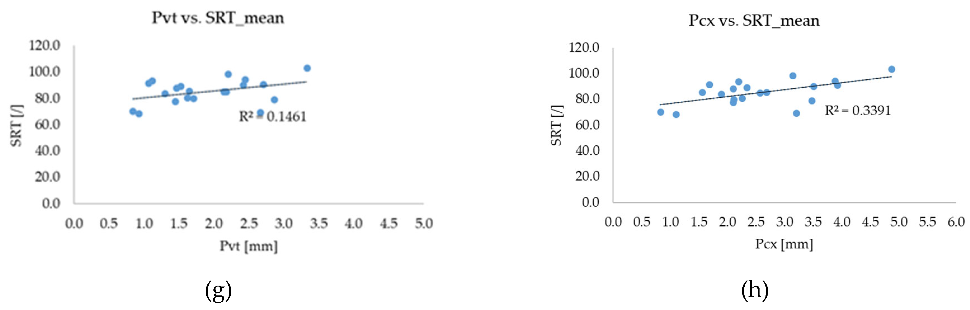
Maximum pit depth [mm]PvtLargest pit depth of all section lengths ls
Mean profile element height [mm]PcMean value of profile element heights Zt for a total number of profile elements
Maximum profile element height [mm]PcxMaximum value of profile element heights Zt for a total number of profile elements
Table 3. Kendall’s correlation coefficients for calculated profile-related texture parameters; highly correlated parameters with Kendall’s coefficient > 0.6 are bold [15].
VariablesPqPskPkuPtPptPvtPzPaPsmPsmxPcPcxMPD
Pq1
Psk−0.2021
Pku−0.198−0.4161
Pt0.827−0.269−0.0551
Ppt0.6740.043−0.3080.6551
Pvt0.726−0.4030.0470.8370.4951
Pz0.835−0.174−0.1940.7920.6790.6921
Pa0.932−0.158−0.2610.7690.6840.6730.8181
Psm0.247−0.1980.0980.2680.1760.2920.1680.2251
Psmx0.190−0.1180.0010.2120.1680.2200.1050.1790.4861
Pc0.834−0.226−0.1520.8020.6340.7350.8170.8080.3000.1861
Pcx0.792−0.271−0.0570.8400.6040.7890.7530.7420.2590.2270.7871
MPD0.7130.031−0.3190.6700.8790.5180.7220.7280.1730.1350.6730.6201
Table 4. Kendall’s correlation coefficients for surface-related texture parameters and measured friction performance SRT value; values in bold are highly correlated with Kendall’s correlation coefficients > 0.6 [15].
VariablesPqPaPzPcPtPptPvtPcxMPDSRTmean
Pq1
Pa0.9681
Pz0.8840.8951
Pc0.9470.9370.9371
Pt0.7370.7260.7470.7891
Ppt0.6320.6630.6840.6420.5371
Pvt0.6320.6210.6000.6630.8110.3681
Pcx0.7790.7680.7680.8110.8740.5160.7891
MPD0.6840.6950.7580.7160.5470.8000.4420.5891
SRTmean0.3890.4210.4840.4210.3580.6530.2320.3580.6631
Table 5. Model parameters and model performance for the initial MLR framework models [15].
Regression ModelModel ParametersAdjusted R2RMSENote
LRMPD0.5926.162Moderate linear relationship between MPD and friction
MLRv1Pa, Pz, Pc, Ppt0.7603.987Pa was found to be statistically insignificant
MLRv2Pz, Pc, Ppt0.7624.581Pa was found to be statistically insignificant, Pc was attributed with a negative coefficient (contrary to the previous correlation analysis where a monotonic positive relationship with friction was detected)
MLRv3Pz, Pc0.7204.970Multicollinearity for predictor variables (VIF > 10), Pc was attributed with a negative coefficient
Table 6. Ridge regression for prediction model establishment.
Regression ModelPenalty TermModel PredictorsAdjusted R2Note
Ridge (k = 5)0.6873Pa, Pz, Pc, Ppt0.6845-fold cross-validation (initial)
Ridge (k = 10)0.5464Pa, Pz, Pc, Ppt0.60010-fold cross-validation (initial)
Ridge (k = 5)V10.6800Pa, Pz, Pc, Ppt0.694Optimization by Z-score test outlier removal, penalty term updated
Ridge (k = 5)V20.812Pz, Ppt0.768Optimization by removal of predictors with negative coefficients (Pa and Pc), penalty term updated
Table 7. Principal component analysis results for four principal components derived as spectral decomposition of original variables matrix [15].
Principal ComponentEigen ValueVariability [%]Pa
Contribution [%]
Pz
Contribution [%]
Pc
Contribution [%]
Ppt
Contribution [%]
PC13.73693.40326.03326.05425.96921.944
PC20.2325.7965.7445.88910.66177.676
PC30.0240.60353.12746.7030.1680.002
PC40.0080.19715.06621.35563.2010.378
Table 8. Results of PCA regression analysis for prediction model establishment [15].
Regression ModelModel PredictorsVIFModel EquationAdjusted R2Note
PCAv1PC1, PC21.040SRT = 85.170 − 1.217 Pa − 1.239 Pz − 2.186 Pc + 11.402 Ppt0.569Initial model with 2 PCs resulted in negative coefficients associated to some predictors
PCAv2PC1n.a.SRT = 85.17 + 1.679 Pa + 1.681 Pz + 1.676 Pc + 1.541 Ppt0.503A Z-score outlier test performed to detect and remove outliers
PCAv3PC1n.a.SRT = 85.8609 + 1.8917 Pa + 1.8937 Pz + 1.8898 Pc + 1.7363 Ppt0.667Final model iteration
Table 9. PLS regression model characteristics for model iterations [15].
Regression
Model
Model
Predictors
LV’s Global
Contribution to the Model
(Q2cumulative)
LV’s Explanatory Power for Model Predictor
(R2Xcumulative)
LV’s Explanatory Power for Model Output
(R2Ycumulative)
Model EquationNote
PLSv1Pa, Pz, Pc, Ppt0.3760.9750.510SRT = 85.17 + 1.6005 Pa + 1.6997 Pz + 1.5177 Pc + 1.8086 PptInitial model with weaker performance than LR model
PLSv2Pa, Pz, Pc, Ppt0.4790.9780.594SRT = 85.9813 + 1.5896 Pa + 1.6786 Pz + 1.5778 Pc + 1.7203 PptA Z-score outlier test performed to detect and remove outliers
PLSv3Pz, Ppt0.6680.9740.784SRT = 85.4377 + 3.9748 Pz + 3.93478 PptOnly predictors with VIP scores > 1 accounted in the model
Table 10. A summary of proposed friction predictive models by feature engineering procedures—model type, model equation, R2 training set, R2 validation set, and RMSE validation set [15].
Regression ModelModel PredictorsModel EquationR2 (Adjusted) Training SetR2 (Adjusted) Validation SetRMSE
Validation Set
RidgePz, PptSRT = 83.928 + 3.762 Pz + 2.899 Ppt0.7740.7674.442
PCAPa, Pz, Pc, PptSRT = 85.8609 + 1.8917 Pa + 1.8937 Pz + 1.8898 Pc + 1.7363 Ppt0.6170.6675.757
PLSPz, PptSRT = 85.4377 + 3.9748 Pz + 3.93478 Ppt0.7390.7804.412
Disclaimer/Publisher’s Note: The statements, opinions and data contained in all publications are solely those of the individual author(s) and contributor(s) and not of MDPI and/or the editor(s). MDPI and/or the editor(s) disclaim responsibility for any injury to people or property resulting from any ideas, methods, instructions or products referred to in the content.

