Abstract
The application of Artificial Neuronal Networks (ANN) offers better statistical accuracy in erosion-corrosion (E-C) predictions compared to the conventional linear regression based on Multifactorial Analysis (MFA). However, the limitations of ANN to require large training datasets and a high number of inputs pose a practical challenge in the field of E-C due to the scarcity of data. To address this challenge, a novel ANN method is proposed, structured to a small training dataset and trained with the aid of synthetic data to produce an E-C neural network (E-C NN), applied for the first time in the study of E-C wear synergy. In the process, transfer learning is applied by pre-training and fine-tuning the model. The initial dataset is created from experimental data produced in a slurry pot setup, exposing API 5L X65 steel to a turbulent copper tailing slurry. To the previously known E-C scenario for selected values of flow velocity, particle concentration, temperature, pH, and the content of the dissolved , new experimental data of stand-alone erosion and stand-alone corrosion is added. The prediction of wear loss by E-C NN considers individual parameters and their interactions. The main result is that E-C ANN provides better prediction than MFA as evaluated by a mean squared error (MSE) values of 2.5 and 3.7, respectively. The results are discussed in the context of the cross-effect between the proposed prediction model and the resulting estimation of relative contribution to E-C synergy, which is better predicted by the E-C NN. The E-C NN model is concluded to be a viable alternative to MFA, delivering similar prediction with better sensitivity to E-C synergy at shorter computation times when using the same experimental dataset.
1. Introduction
In the mining industry, slurry pipeline systems are the most cost-effective solution for long-distance transport of large quantities of particulate solids. However, due to the nature of the carrier fluid, one of the main threats to a pipeline system, consisting of pipes, pumps, valves, etc., is the degradation by erosion and corrosion processes acting simultaneously in a synergistic phenomenon referred to as erosion-corrosion (E-C). In this context, the challenge is to keep the pipeline integrity to prevent failures that can result in leakage accidents [1] affecting nearby communities and the environment.
In metallic materials, the wear rate of E-C is defined by the weight loss of the material due to the physical damage induced by solid particles impacting over the surface and by the corrosion mechanisms that involve ionic exchange between the surface and the carrier fluid (electrolyte). In this process, the erosion mechanism is enhanced by corrosion and vice versa through a complex synergy resulting in E-C weight loss higher than the sum of losses by erosion and corrosion separately [2]. The latter is often described in terms of weight loss by Equations (1) and (2):
where and S describe the total weight loss by E-C, weight loss by sheer mechanical erosion (stand-alone erosion), weight loss by sheer electrochemical corrosion (stand-alone corrosion), and weight loss attributed to the synergy effects, respectively. The synergy S can be further decomposed into erosion-enhanced corrosion () and corrosion-enhanced erosion ().
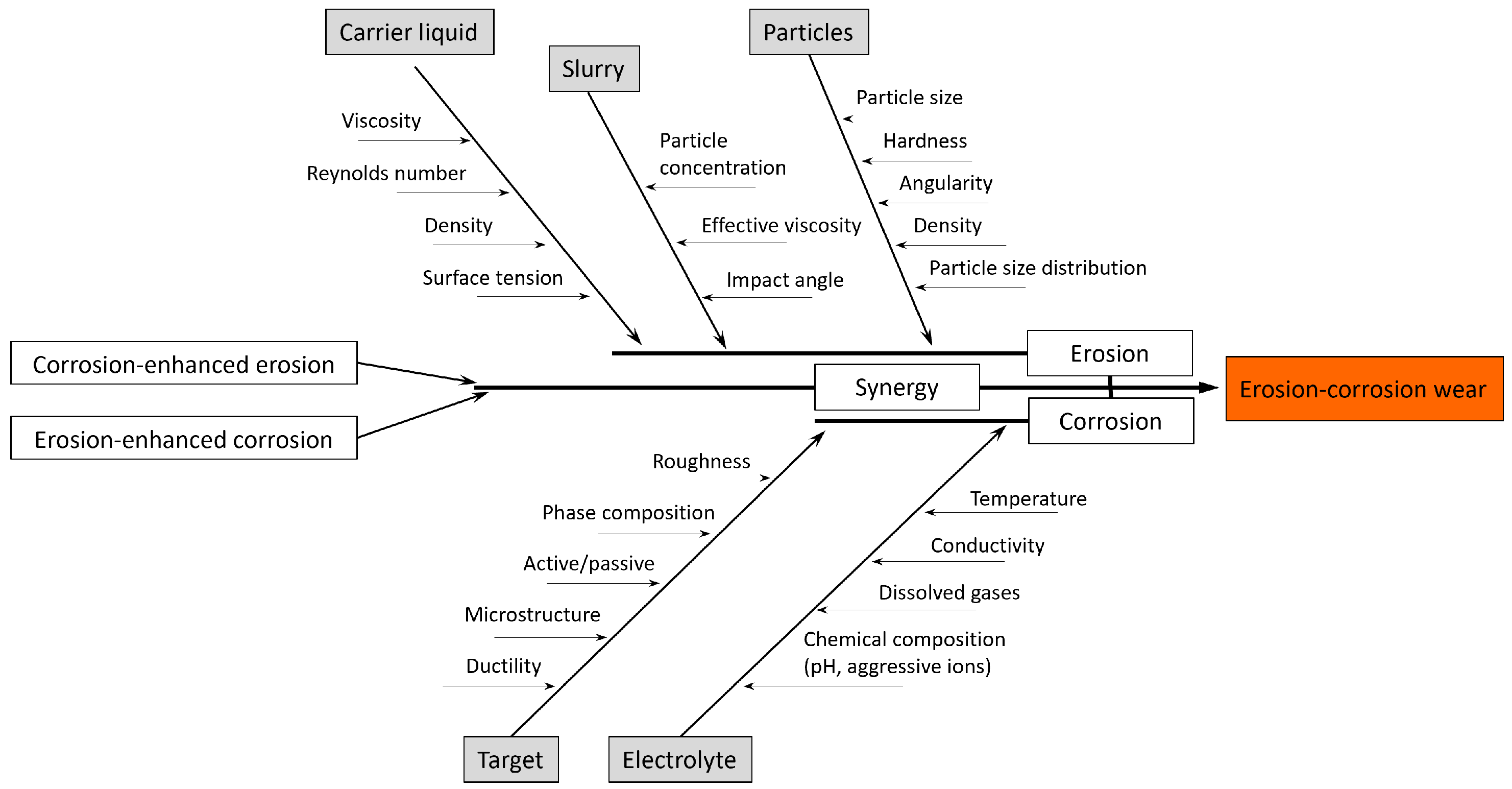
A full description of the E-C phenomenon involves a comprehensive analysis of individual mechanisms as well as their synergistic effects, which can be done in terms of key variables. These variables can be categorized as those proper of the target material and those proper of the slurry, comprising the carrier fluid and the suspended particles. Because the carrier fluid is in motion, its characteristics both as a mechanical medium and as an electrolyte must be distinguished. A summary of all the variables relevant for the modeling of erosive wear was presented by Javaheri et al. [3]. In this work, we extend the scope of relevant variables to explicitly include the synergy with corrosion by compiling E-C data from the literature [4,5,6,7,8,9,10,11,12,13,14,15,16,17,18,19,20], resulting in the fishbone diagram shown in Figure 1.

Figure 1.
Summary of variables relevant to Erosion-Corrosion (E-C) wear.
Because of the apparently unpredictable nature of the wear caused by E-C, it is considered mandatory to develop a prediction tool capable of estimating the wear rate of materials exposed to slurry flow. The currently used models have not proven sufficiently accurate in estimating the service life of slurry transport systems and even revision of design standards has been advised [21]. However, description of physical problems, such as wear, commonly involves a deterministic approach, relying on the physical laws and structure–property relations. Due to the complex nature of the E-C mechanism, a fully deterministic model for accurate prediction of wear rate remains elusive. Alternative approaches include stochastic, e.g., [22,23,24,25], or statistical modeling. The latter relies on establishing correlations between key variables to create a multi-factorial predictive framework. These empirical models, although not including the physics of the phenomena, allow for gaining insight into the interdependence of factors contributing to the E-C phenomena. By analyzing the statistical relationships between principal variables, predictions and effective mitigation strategies can be developed.
The conventional linear regression for multi-factorial analysis (MFA) and response surface method (RSM) has been primarily applied to the study of E-C phenomena, but recent studies have demonstrated the potential of Artificial Intelligence (AI)-based prediction methods, particularly Artificial Neural Networks (ANN), in producing better predictions in terms of statistical accuracy [26,27,28,29,30]. This method has gained popularity in various research areas with applications such as financial analysis, logistics management, weather predictions, etc., showcasing successful outcomes [31] with a substantial number of variables. However, when employing these new AI-based techniques to E-C wear, two main challenges arise: the requirement for large training datasets and a high number of inputs. These restrictions present a significant challenge because scarcity of available data is owed to the substantial time and resource costs associated with its production [32,33]. This is an inherent restriction, the impact of which should be evaluated for each particular application. Whereas AI-enhanced models have been shown to be applicable in the study of friction, wear, and roughness evolution [34], which involve physical mechanisms relevant to E-C, it is estimated as worthwhile to explore and validate its effectiveness specifically for E-C phenomena.
Whereas machine learning (ML) models have mostly been employed in laboratory settings to predict abrasion wear measured by pin-on-disc set-up [32], a significant knowledge gap emerges when it comes to their direct application in comprehending E-C wear mechanisms, particularly in the complex context of turbulent environments. Furthermore, there remains an unaddressed challenge concerning the scarcity of data for neural network applications in wear problems. Additionally, existing E-C wear studies are often reliant on MFA, a tool valued for its capacity to elucidate variable relationships but found lacking in robustness in predictive interpolation. Both these gaps underscore the need for novel approaches and models within the field. In this context, the present work introduces a novel approach to predicting E-C wear by comparing the effectiveness of ANN and MFA based on linear regressions. The method involves developing an ANN-based predictive model tailored for small training datasets and exploring its applicability for extreme cases of factor combinations. In particular, it is hypothesised that ANN can predict the E-C rate with higher accuracy than the conventional MFA approach on the same E-C dataset. The previously published experimental E-C dataset [35] is now expanded by incorporating data of stand-alone erosion and stand-alone corrosion measured in a slurry pot configuration for six parameters: flow velocity, particle concentration, temperature, pH, oxygen content, and copper ion content. Both the MFA and ANN models are utilized to predict wear loss, considering the individual contribution and interaction of the parameters. To overcome the limited experimental data, a synthetic dataset is generated by interpolating factors and incorporating predictions from the MFA model. This approach is equivalent to the data augmentation strategy in ML applications used when there are missing data, unbalanced data, under-sampling, or small dataset problems [33]. This synthetic dataset is then used to pre-train the ANN, followed by fine-tuning using the experimental data. The performance of the MFA and ANN models is compared for stand-alone erosion, corrosion, and combined E-C scenarios. Finally, the relevance of the results is discussed regarding the relative contribution of synergistic factors.
2. Experiment and Methods
The present study builds on the experimental data of E-C weight loss reported by Aguirre et al. [35] along with their MFA. The experimental extension consists of including new data for the stand-alone erosion and stand-alone corrosion mechanisms for E-C wear weight loss, while maintaining the same levels of the original studies’ variables which are presented in Appendix A. This extension completes an experimental dataset that establishes the relationship between the controlled variables of flow velocity (V), particle content (P), temperature (T), , content of dissolved oxygen (), and content of copper ions (), and their influence on the effective wear rate, encompassing E-C and the stand-alone corrosion and erosion. Then, through regression analysis, empirical models are derived from the dataset to interpolate the variables and generate a larger dataset. This expanded dataset is used to create and pre-train a Deep Learning Neural Network (DLNN). Subsequently, transfer learning is applied to fine-tune the DLNN using the experimental data. The entire workflow is summarized in Figure 2.

Figure 2.
Summary of the work flow, from collection of experimental E-C data to performance evaluation through MSE.
2.1. Experimental Determination of E-C Wear
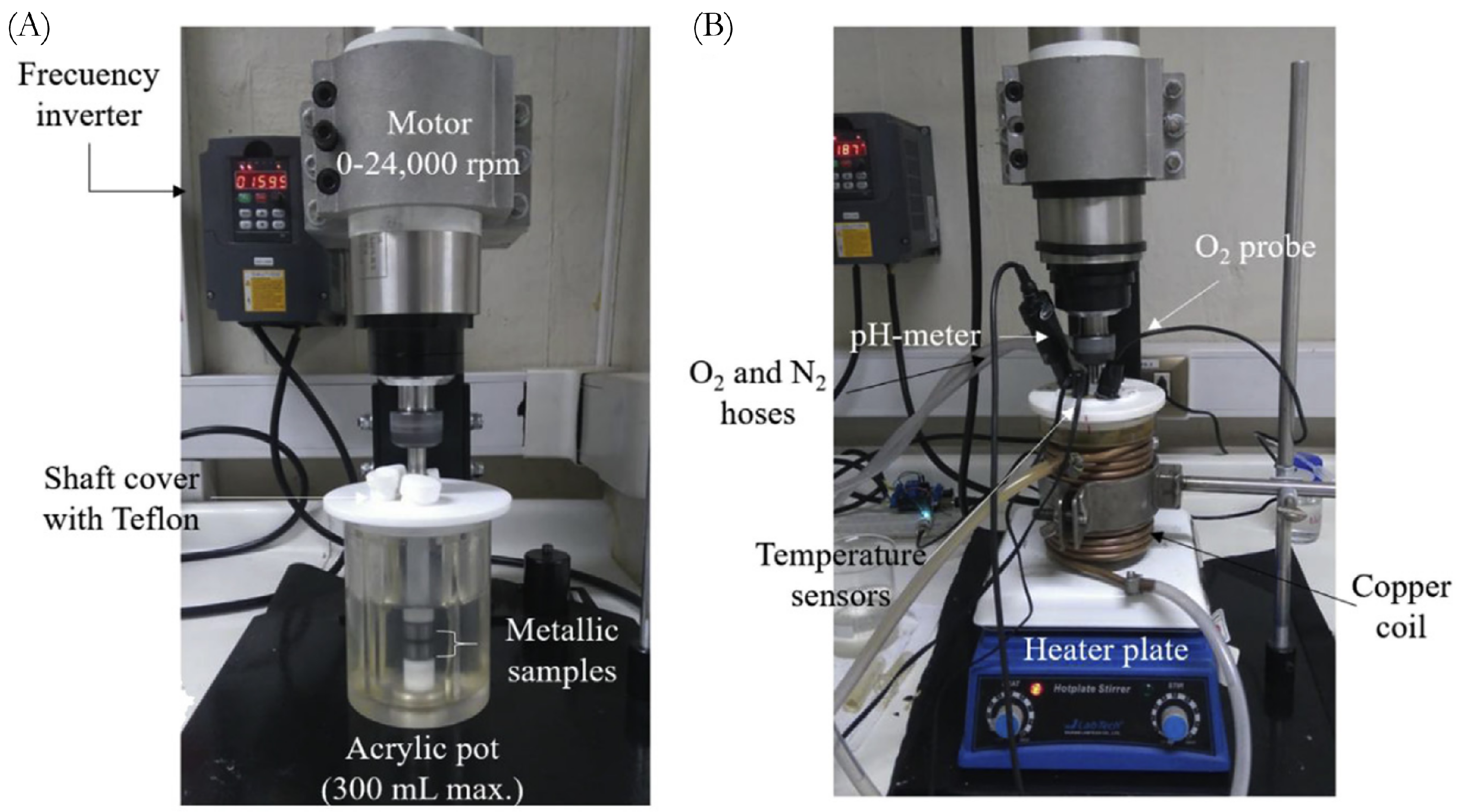
The experiment for measuring the weight loss of stand-alone corrosion and stand-alone erosion was carried out using the same experimental setup and materials as those reported by Aguirre et al. [35]. The target material were sample cylinders of API 5L X65 steel of 15 mm in diameter and 10 mm in height. Before conducting the experiments, the API 5L X65 cylinder samples were prepared, polishing their surface with SiC paper, starting from 320 to 1200 grit, and then thoroughly cleaning them with ethanol in an ultrasonic bath to remove any contaminants. The cleaned samples were then weighed using an analytical balance with a precision of 0.1 mg to obtain their initial weight, ensuring accurate measurement of weight loss during the test. The cylinders were mounted at the rotation axis of a rotating cylinder electrode (RCE) setup (Figure 3A), allowing for separation of erosion from corrosion via electrochemical polarization. The stand-alone erosion measurements were carried out with the corrosion suppressed by applying −1.2 V vs. Ag/AgCl (cathodic protection) to the target material. The stand-alone corrosion scenarios were implemented by not adding the solid particles.
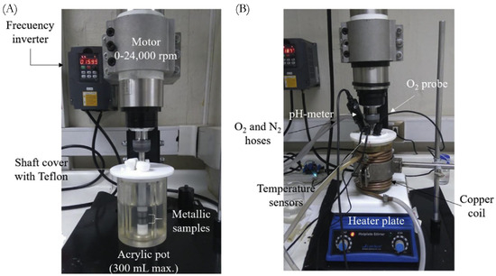
Figure 3.
Experimental slurry pot: (A) overview of the RCE set-up with location of the test sample in a pot filled with water for visibility and (B) complete configuration for controlling all the studied factors. Adapted from [35].
The electrolyte used for preparing the slurry was prepared using distilled water, sulfuric acid, and sodium hydroxide in concentrations necessary to produce and maintain the desired pH during the exposure. The values of the pH, temperature, and content of Cu ions were selected to be relevant for realistic operating environments. The duration of exposure to erosion or corrosion was 75 min. After exposure, the samples were removed and immediately cleaned to remove any residual deposits or contaminants that may have adhered during exposure. The cleaning procedure consisted of an ultrasonic bath of the samples for 180 s, first in acetone and then in an inhibiting acid solution (Clark solution consisting of 1000 mL of hydrochloric acid, 20 g of antimony trioxide (Sb2O3), and 50 g of stannous chloride (SnCl2)) according to the ASTM standard G1-03 [36]. The cleaned samples were then carefully weighed again to determine the weight loss. The variability of the difference in weight before and after exposure was determined to approximate the statistical experimental error of E-C, stand-alone erosion, and stand-alone corrosion, which were found to be 0.078, 0.173, and 1.292 mg·cmh, respectively.
2.1.1. Experiment Design
The test parameters used in the fractional factorial design of the experiments are summarized in Table 1, indicating the lowest, central, and highest values assigned to each parameter. The specific values were chosen to cover the range of conditions met during the practice of handling the slurry from the copper tailing. In particular, the high levels of P and ions correspond to the worst-case scenario of the residual copper in the tailing. The high and low levels of dissolved oxygen correspond to fully oxygenated and oxygen-free electrolytes, respectively, mimicking the oxygen consumption in a closed system handling slurry.

Table 1.
Summary of test parameters used for the fractional factorial design of experiment, indicating the lowest, central, and highest values.
The design included stand-alone corrosion and erosion experiments. A total of 105 observations are resultant, with 35 observations for each experiment, including the earlier E-C experiment conducted by Aguirre et al. [35] and included in Appendix A Table A3. Each set of the 35 runs included 32 distinct factor combinations, as well as one combination representing the factors’ central values. In addition, two replications of the central combination were added to assess the variability of the results and explain the intrinsic experimental error. For instance, in stand-alone corrosion, the particle concentration factor (P) is irrelevant and has been set to 0 since there are no particles involved. Similarly, in the case of stand-alone erosion, factors such as pH, (P× Cu concentration, and dissolved oxygen () are not relevant. The experimental results for E and C results are presented in Appendix A Table A1 and Table A2 respectively.
2.1.2. Multifactorial Analysis of Experimental Data
The experimental results from Table 1 were used to construct a response surface and develop a polynomial model for predicting wright loss in relation to stand-alone erosion and stand-alone corrosion as schematized in Figure 4. Estimation of weight loss within the range of the input factors was obtained by fitting the experimental data to a polynomial equation as an output of the multifactorial analysis. The relationship between the input factors and the resulting erosion and corrosion effects is then quantified by the coefficients of the polynomial equation, expressing the relative importance of each factor.

Figure 4.
Schematic representation of generating the empirical model by MFA using experimental data.
The analysis was conducted using the R programming language [37] with specific libraries to handle the data and calculate the main factor contributions. The “Dplyr” and “FrF2” [38] libraries were used to process the experimental data and assess the key factors’ impacts. Additionally, the ” Leaps” [39] library, along with the “regsubsets” function, was used to determine the best linear regression fitting. This process involved optimizing the output polynomial by considering the most significant factors based on Mallows’ Cp [40] and Schwartz’s information criterion (bic) [41]. These criteria were essential for selecting the most relevant factors and obtaining an accurate regression model for the data. Finally, the fitting metrics, the multiple R-squared value, and the adjusted R-squared value have been obtained using the “lm” function contained in the R language default libraries.
2.2. E-C Neural Network
The model of E-C wear based on the neural network was obtained by the development of model architecture, followed by transfer learning consisting of stages of pre-training and fine-tuning. Since the amount of experimental data was insufficient for developing an NN model, synthetic data were generated in addition.
2.2.1. Model Architecture
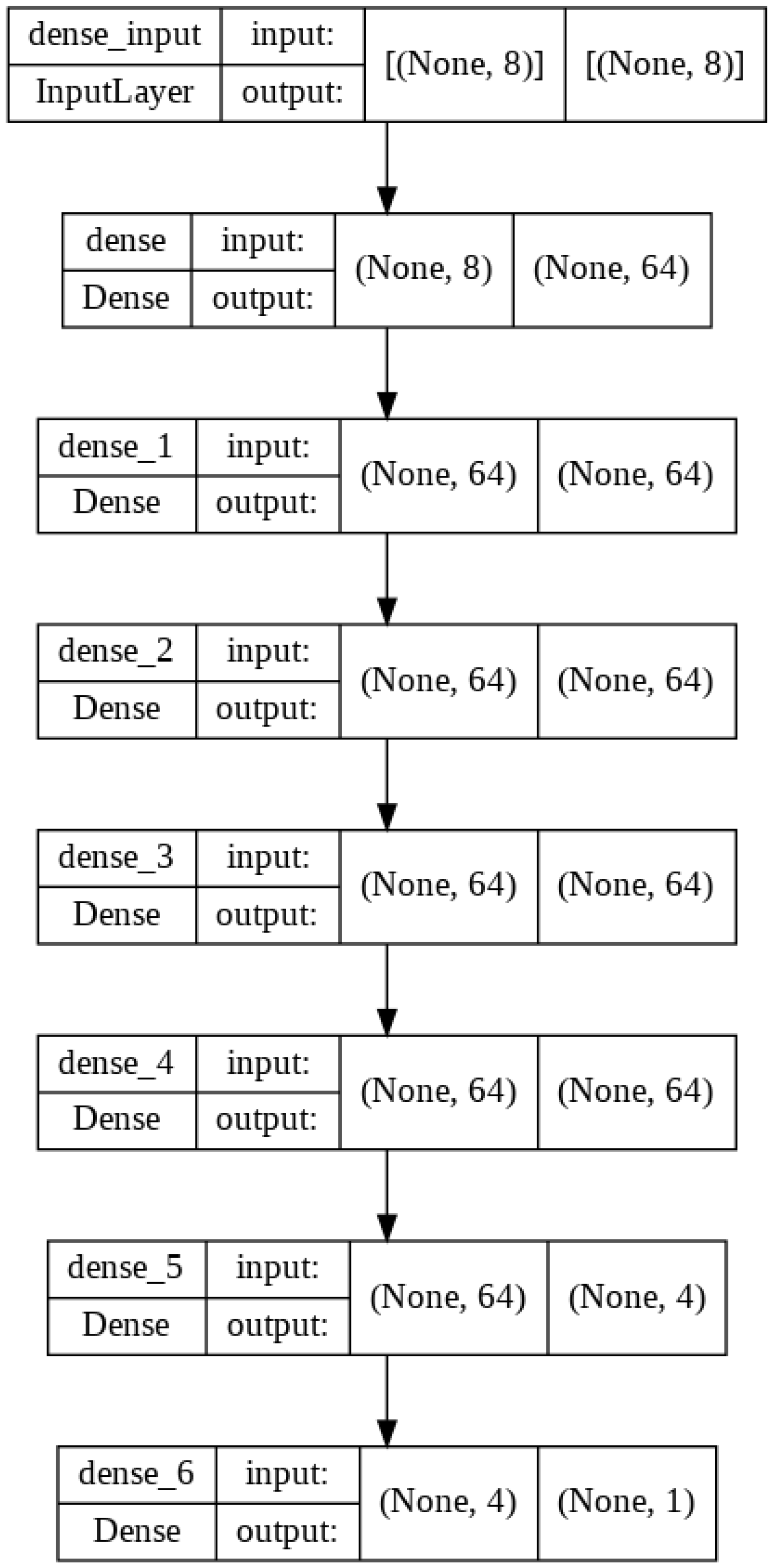
In this study, the GridSearchCV tool from the Scikit Learn library [42] was used to generate and assess various combinations of hyperparameters, i.e., the main parameters used for setting up the NN. The hyperparameter grid encompassed options for the number of layers (ranging from 2 to 6), number of nodes in the first layer following the input layer (128, 64, 32, and 16), a single node in the last layer to select particular mode (erosion–corrosion, erosion, corrosion), activation functions (sigmoid, relu, tanh, and softmax), loss functions (Poisson, Hinge), and batch size (3 and 10). The optimal architecture was determined using experimental data, as schematized in Figure 5. The selection of this architecture was guided by its ability to accurately model and predict E-C wear within the particular context of this study. It represents the combination of hyperparameters that demonstrated the highest performance and predictive accuracy for the weight-loss data.
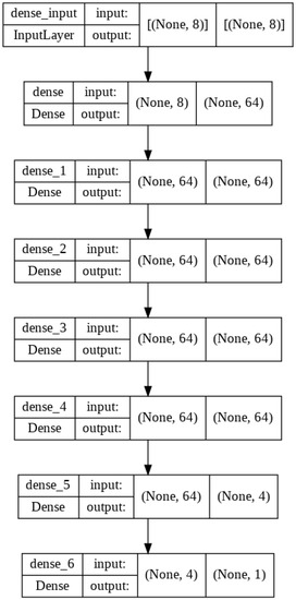
Figure 5.
Schematic representation of the NN architecture after GridSearchCV optimization process.
The input layer and output layers were defined by the experimental problem, with six input parameters available in this case to derive one output parameter (wear rate). In order to facilitate a more efficient convergence and improve the accuracy of the NN model, two additional input parameters were incorporated: corrosion activation and erosion activation (attaining the value of 0 or 1 for deactivate or activate, respectively), obtaining eight input parameters in total. Although these parameters do not have the physical meaning of an experimental factor, they are crucial in enhancing the model’s performance by adding information on whether the combination of input factors corresponds to the experimental run of stand-alone erosion, stand-alone corrosion, or the full E-C scenario. The inclusion of corrosion and erosion activation parameters aids the learning process of the NN because these parameters act as conduits, facilitating exploration of the input space and accelerating the convergence of the model’s results. Their presence helps the NN to better model complex interactions between the different wear mechanisms in the sense that faster convergence and enhanced overall predictive capability of the network is observed.
2.2.2. Pre-Training Using Synthetic Data
The training process employed a two-step approach to optimize the NN model’s performance. In the initial step, the model was pre-trained using an extended dataset that combined the original experimental data with synthetically generated ones. The pre-training phase provided the model with a broader scope of E-C patterns by exposing it to the most diverse range of scenarios represented in the synthetic data.
The original dataset consisted of 105 observations, with 35 observations per E-C, stand-alone erosion, and stand-alone corrosion, respectively. In order to enhance the dataset and capture a broader range of variations, 1395 synthetic data points were generated, resulting in a consolidated dataset of 1500 observations. The synthetic data were included to ensure a comprehensive dataset for training the ANN model. The synthetic data were generated by fitting a robust polynomial model derived from the results of stand-alone erosion and stand-alone corrosion experiments, as well as the erosion–corrosion findings. This polynomial model provided an effective means of interpolating the experimental data and extrapolating them to unexplored regions of the input space, as shown schematically in Figure 6.

Figure 6.
Schematic representation of generating synthetic data using not measured values of factors (*) in the range of experimental factors except for the very experimental values.
The synthetic data set were used for the pre-training stage, and in this case only, was divided into subsets of Training (75%) and Validation (25%) in order to find the best epoch number to avoid an overfitted model. For the resulting architecture, the best relationship on MSE between Training and Validation was in the 135 epoch, obtaining a validation MSE of 2.5 at epoch 135 and MSE of 17.9 at epoch 136, which is indicative of a starting point of overfitting for this synthetic dataset.
2.2.3. Fine-Tuning, Validation and Evaluation
After pre-training, the model underwent fine-tuning using a curated dataset derived solely from the original experimental data, without any synthetic data. The aim of fine-tuning was to improve the model’s performance and enable it to capture the specific nuances and characteristics present in the experimental conditions. Progress during the fine-tuning process was monitored through a validation subset to minimize prediction errors. The E−C NN model resulting from this process was then evaluated using a separate test subset.
The experimental dataset, consisting of 105 observations, was first shuffled to ensure randomness and eliminate potential bias. The shuffled dataset was then divided into three subsets: 50% for fine-tuning training (53 observations), 25% for validation (26 observations), and 25% for testing (26 observations).
During the fine-tuning process, the model learned from the input–output patterns in the data and adjusted its internal parameters to minimize prediction errors until reaching a satisfactory level of convergence.
The validation subset served as an independent dataset to assess the model’s performance during training. However, as it is incorporated into the training process, its evaluation can become biased. To provide an unbiased evaluation of the model’s performance, the testing subset was used as a benchmark. This subset allowed assessment of the model’s ability to accurately predict E-C weight loss using unseen data, providing insights into its reliability and robustness.
For the fine-tuning stage, the model was trained during 50 epochs, which was the optimum for this hyperparameter delivered by the GridSearchCV algorithm [42] without producing overfitting. The MSE values obtained during the validation stage and for the test sub-dataset were 3.6 and 6.9.
2.2.4. Sensibility Analysis of E-C NN
To analyse the sensitivity of the E-C NN model to each parameter, a systematic process was followed. The training and fine-tuning process for the E-C NN model was repeated 34 times, with each iteration predicting the wear rate for all experimental combinations. After obtaining the 34 predictions for the experimental wear rates, the results were averaged to obtain a single prediction for each wear rate.
Next, the average prediction was evaluated using the fractional factorial design algorithm to assess the independent effects of each factor on the E-C, erosion, and corrosion as stand-alone wear rate and to be comparable with the main effects of experimental factors. This analysis allowed us to understand the individual contribution of each factor and their significance in influencing the wear rate. It is important to remark that the most relevant factors to E-C were identified as the parameters that exhibited the most significant changes in the predicted weight loss.
3. Results
3.1. MFA Model of E-C Wear
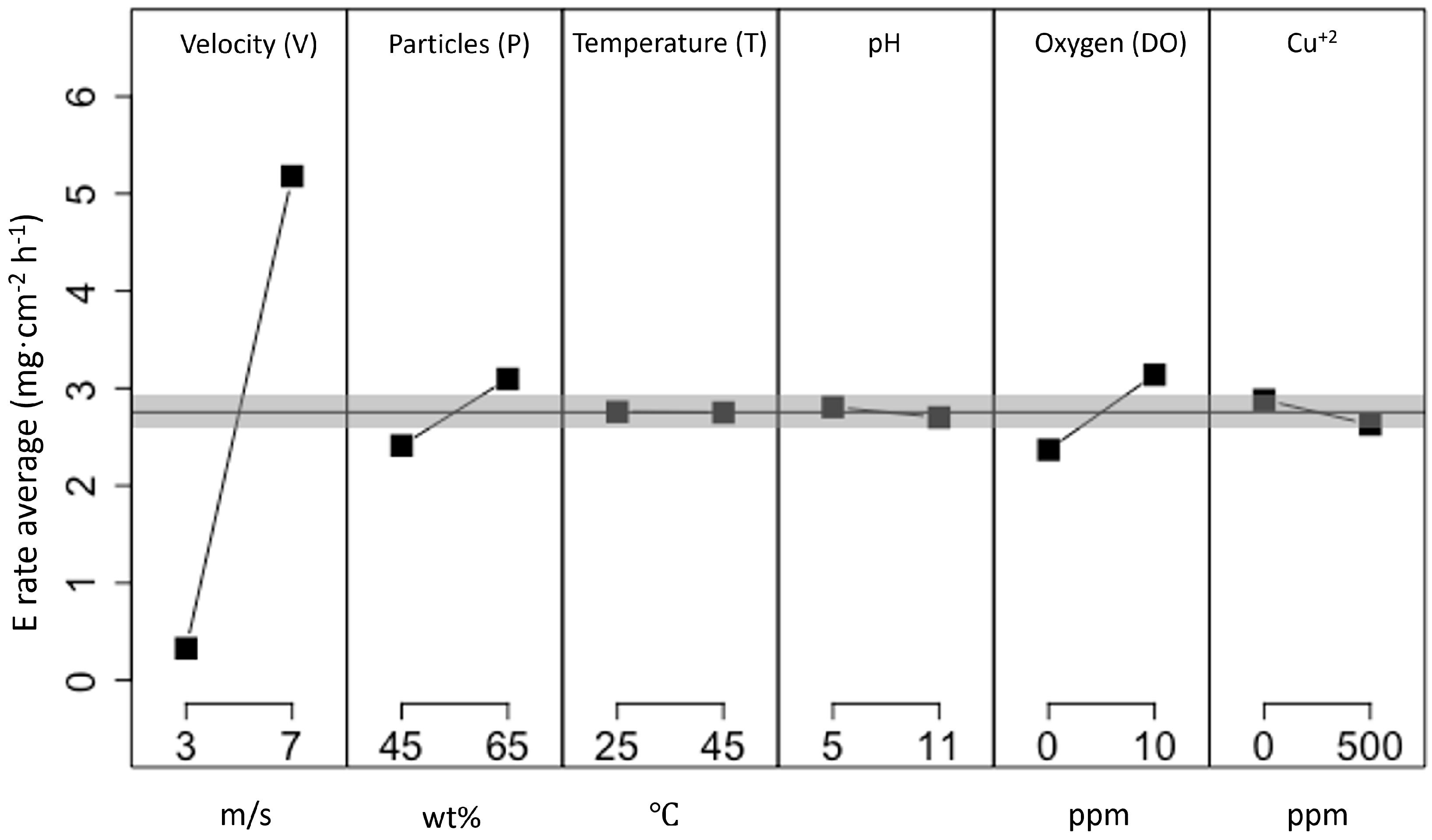
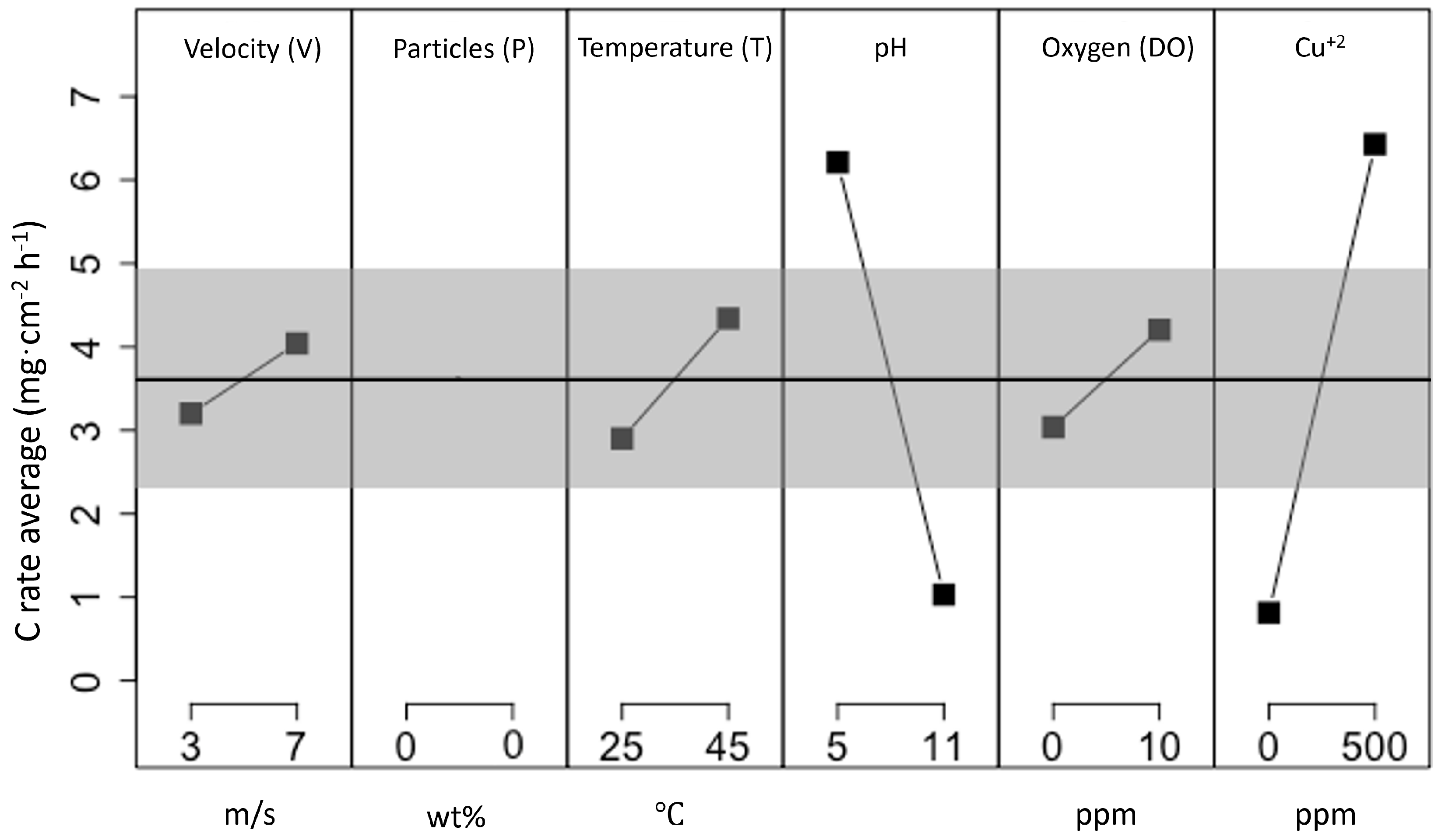
Figure 7 summarizes the main effects of E-C obtained experimentally by Aguirre et al. [35], demonstrating that the velocity (V), temperature (T), and content of dissolved oxygen () are the significant factors as determined by MFA (Equation (3)):
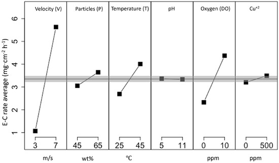
Figure 7.
Main effects of experimental factors on the E-C rate. The range of experimental standard deviation is marked in gray. Adapted from [35].
The derived equation represents a parametric relationship between the E-C rate and the importance of the influencing factors. The units of the variables are summarized in Table 1. The units of the coefficients are chosen to rescale the respective variable to the units of wear rate ((mg·cmh)). Positive coefficients indicate a positive correlation, suggesting that an increase in these factors leads to an increase in the E-C wear rate. Conversely, negative coefficients indicate a negative correlation, indicating that an increase in those factors results in a decrease in the E-C rate. The interaction terms, such as () and (), take into account the combined effects of multiple factors on the E-C rate, which can be either synergistic or antagonistic when positive or negative, respectively. The variability of the E-C rate determined for the standard deviation of the central levels is approximately 0.078 (mg·cmh), which is comparable to the statistical error of the experiment, visualised in Figure 7 as a gray band. This indicates that the obtained results are reliable and within an acceptable range of variability. An extended description of the experimental procedure, data collection, data analysis, and the derivation of the MFA model is provided in the work of Aguirre et al. [35].
3.2. MFA Model of Stand-Alone Erosion Wear
In an analogy to the E-C main effects shown in Figure 7, the results specific to stand-alone erosion are presented in Figure 8. The experimental standard deviation of the erosion data is approximately 0.173 (mg·cmh), which is higher than that of the E-C data. The significant main effects are those of velocity, particle content (P), and oxygen content ().

Figure 8.
Main effects of experimental factors on the stand-alone erosion rate. The range of experimental standard deviation is marked as a gray stripe.
The linear model of stand-alone erosion with second-order terms obtained in an analogy to Equation (3) by MFA is given by Equation (4):
The residual standard error of this fitted erosion MFA model is 1.328 (mg·cmh), the multiple R-squared value is 0.8438, and the adjusted R-squared value, accounting for the number of predictors and degrees of freedom, was calculated to be 0.8276. The average deviation of the observed erosion rate values from the predicted values indicates that approximately 84.38% of the variability in the erosion rate can be explained by the model. The metrics suggest that the linear model with second-order terms provides a reasonable fit to the data, as evidenced by the relatively low residual standard error and high R-squared values. The experimental error visualised in Figure 8 as a gray band indicated that the effect of the temperature and content of is not relevant.
3.3. MFA Model of Stand-Alone Corrosion Wear
The main effects of factors in the corrosion experiment were analysed analogously to those of the E-C and stand-alone erosion scenarios. The results are summarized visually in Figure 9 and the linear model with second-order terms for the stand-alone corrosion is given by Equation (5):
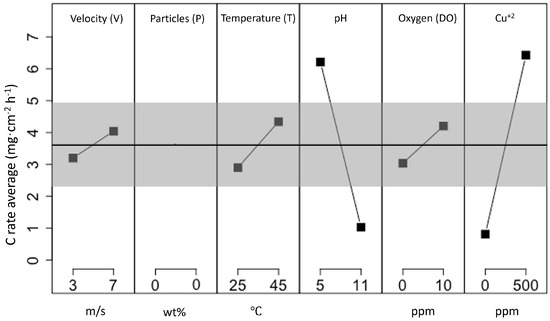
Figure 9.
Main effects of experimental factors on the stand-alone corrosion rate. The range of experimental standard deviation is marked in gray.
The experimental variability of the corrosion rate at the central levels was assessed by the standard deviation to be approximately 1.292 (mg·cmh), which is notably higher than that of E-C and stand−alone erosion. Considering the experimental error visualised in Figure 9 as a gray band, the significant main effects are only those of and the content of the dissolved (). The metrics of the fitted corrosion MFA model are a residual standard error of 2.324 (mg·cmh), multiple R-squared value of 0.8821, and adjusted R-squared value, accounting for the number of predictors and 28 degrees of freedom amounting to 0.8526.
3.4. E-C NN Model Predictions
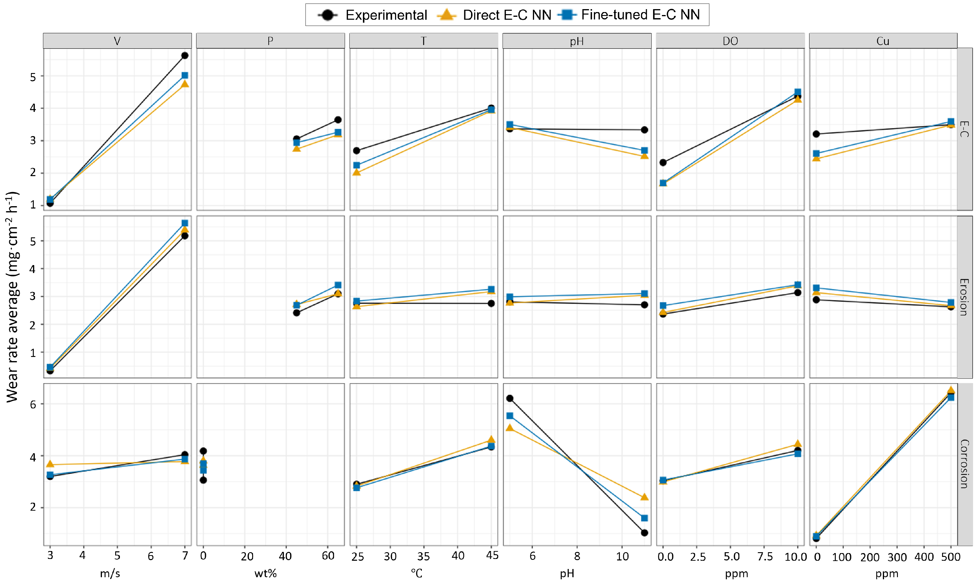
Figure 10 summarises the results of the E-C NN model predictions in comparison with the experimental data of the E-C rate and the stand-alone erosion and corrosion rates. The effect of transfer learning is visualised by considering the direct E-C NN and the fine-tuned E-C NN. In general, the tendencies of all the main effects are correctly predicted by the E-C NN model; however, the slopes differ slightly. The slopes produced by the fine-tuned model are closer to the experimental data, which is particularly evident in the case of the E-C predictions. The effect is less pronounced in the case of stand-alone erosion, whereas for the stand-alone corrosion there is almost no effect of transfer learning except for the pH factor, in which fine-tuning provides notably better prediction.
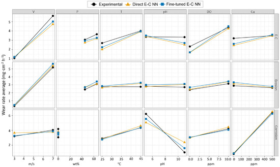
Figure 10.
Effect of pre-training on the prediction of the rates of E-C (upper row), stand-alone erosion (middle row), and stand-alone corrosion (bottom row) for the main factors as compared to the experimental values.
The effect of the particles on stand-alone corrosion is included to represent the statistical error, as this is the physical meaning of corrosion weight loss in the absence of abrasive particles. In the case of the experimental data, the statistical error represents the experimental accuracy.
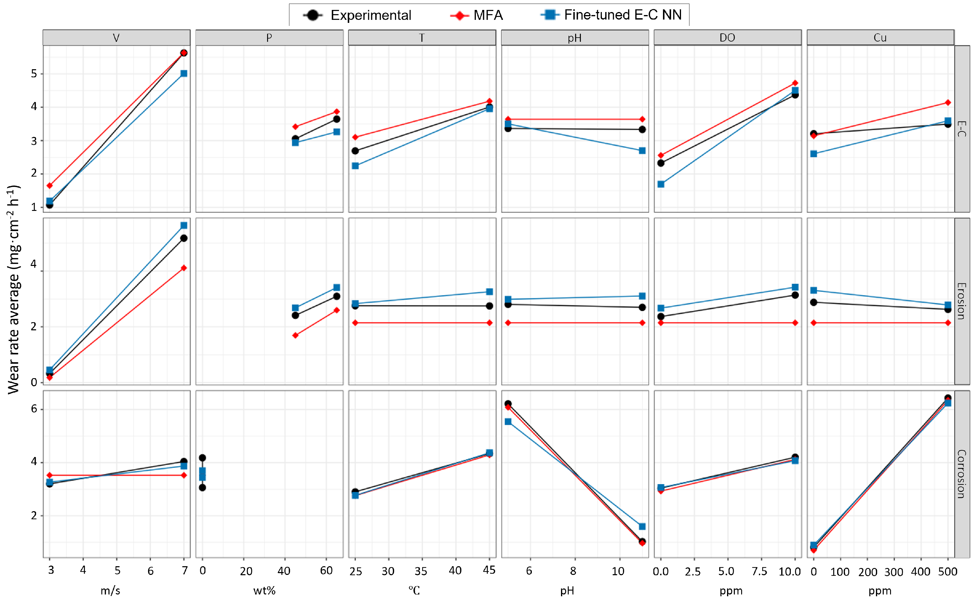
The predictions of the fine-tuned E-C NN model are compared with the MFA predictions and experimental data in Figure 11. In general, both models produce the same tendencies for all the factors, but the values predicted by the E-C NN are closer to the experimental ones as compared to the MFA model. This effect is most notable in the case of stand-alone erosion, in which the weight loss is systematically underestimated for all the factors.
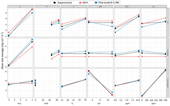
Figure 11.
Comparison of main effects of experimental factors on the wear rate of E-C (upper row), stand-alone erosion (middle row), and stand-alone corrosion (bottom row) as determined by the experiment, MFA, and pre-trained E-C NN.
4. Discussion
4.1. Validity of Synthetic Data
Due to the multi-factor nature of the E-C wear (Figure 1) MFA models have been the method of choice to describe the E-C process. However, availability of experimental data is restricted because of the involved effort, considering that the results are specific to particular experimental set-ups [3]. In addition, to assure applicability of results to actual slurry handling systems, the design of experiments is restricted to the range of parameters of practical interest rather than relevance for the relative importance of the mechanisms of wear loss. In this context, generation of synthetic data from MFA model corresponds to the current practice in predicting wear rate. The synthetic data are then the best interpolation between the measured values.
In this work, a comprehensive MFA model of E-C wear is presented, i.e., derived from the data considering both E-C (Equation (3)) and the stand-alone erosion and corrosion scenarios (Equations (4) and (5), respectively). The inclusion of synergy-free scenarios of erosion and corrosion resulted in models not capable of predicting the very values measured experimentally (see Figure 11). The deviation is particularly notable in the case of stand-alone corrosion, where even the sign of the wear rate was changed from weight loss (experiment) to weight gain (MFA model). This observation is attributed to the limited capacity of MFA to capture a possible shift in the dominant mechanism of wear or the rise of synergy. The complexity of the involved physical, chemical, and mechanical processes, although generally acknowledged, has not been studied sufficiently to provide an analytical description of each mechanism. The lack of mechanistic descriptions hinders the evaluation of the validity of the synthetic data, as a monotonic response of the system at the intermediate values is inherently assumed. However, for the purpose of the current work, and for a lack of reason to assume otherwise, the synthetic data derived from the MFA model are considered sufficiently valid.
The accuracy of the MFA model certainly depends on the experimental error. Although all the weight loss data were measured using the same analytical balance, the statistical error of the stand-alone corrosion data is notably higher than that of erosion-corrosion and stand-alone erosion data. This error is mostly explained by the outlier data point measured for high velocity (7 m/s), low particle concentration (45 wt.%), high temperature (45 °C), low pH (5), high content of dissolved oxygen (10 ppm), and high content of dissolved (500 ppm), which correspond to aggressive combination parameters indicating a possible shift in the mechanism of E-C wear as discussed by Aguirre et. al [43]. Nonetheless, the accuracy of the MFA model (1.922 (mg·cmh)) is higher than the statistical error of the experiment (1.292 (mg·cmh)), justifying at least the validity of the synthetic data.
Notwithstanding the above discussed limitations, by combining the experimental data with the synthetic data, the dataset became more diverse and representative of a wide range of E-C scenarios. This augmentation of the dataset was necessary for the NN model to learn from a broader spectrum of conditions, enabling it to generalise better and make more accurate predictions.
4.2. Applicability of E-C NN
The E-C NN model was developed using experimental and synthetic data, which were separated into subsets used independently to train and evaluate the model. In addition, development of the model comprised the approach of transfer learning, consisting of pre-training followed by fine-tuning. By combining the pre-training with synthetic data and subsequent fine-tuning with a small dataset from the experiments, the NN model could leverage the advantages of both data types. In other words, the pre-training provided the model with a “fundamental understanding” of E-C behaviour, whereas the fine-tuning aligned the model’s predictions with real-world scenarios of the specific case as shown in Figure 10. As result, the fine-tuned E-C NN predicts the wear rate of a determined system better than MFA, as shown in Figure 11.
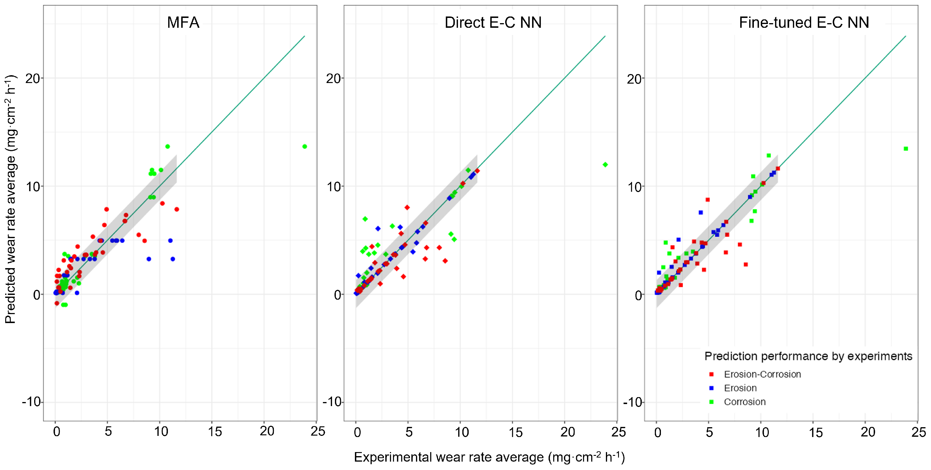
Overfitting of the E-C NN model model was avoided at the stage of fine-tuning. Indeed, there is no evidence of global overfitting as a validation MSE of 3.9 and the overall prediction MSE of 2.4 were observed. It is noted that in Figure 12, certain data points appear to be closer to zero error, indicating the possibility of localised overfitting. However, the overall model does not exhibit signs of overfitting. The absence of overfitting indicates that the model was able to generalise well, without overemphasizing the noise or irrelevant patterns in the data.
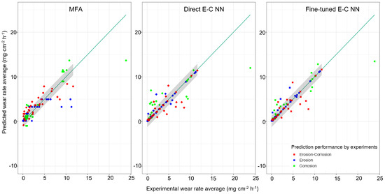
Figure 12.
Comparison of accuracy in predicting experimental values of wear rate by the MFA and E-C NN models (direct and transfer learner). Each data point corresponds to an experimental run. The gray area represents standard deviation due to experimental error. The green line is added as guide for the eye to represent perfect prediction.
Figure 12 compares the performance of the MFA and E-C NN model, both direct and fine-tuned, and Table 2 compares the statistics of the models’ predictions in terms of squared error. In general, the fine-tuned E-C NN provides the best prediction as expressed by the mean squared error of 2.535 compared with 3.694 for the MFA model. Notably, the mean error of the direct E-C NN model is similar to that of the MFA, but with a significantly lower median of 0.019 as compared with 0.345 for the MFA.

Table 2.
Tabulation of squared errors of the MFA and E-C NN model predictions shown in Figure 12.
The fine-tuned E-C NN model demonstrates a superior capability for predicting wear rate as compared to the MFA models applied directly to the experimental E-C data. Moreover, the E-C NN model is able to capture complex relationships and non-linearities in the dataset, which is evident in the velocity parameter (V). This parameter in the MFA was introduced using squared velocity to have better fitting, with the rationale that erosive wear is mostly caused by the transfer of kinetic energy, which is proportional to rather than V [44]). In the case of E-C NN, no such introduction was necessary because the model is capable of inferring this relation, highlighting the advantage of ANNs in modeling intricate patterns not necessarily captured by a conventional MFA model. Interestingly, even the direct E-C NN model, i.e., without transfer learning, outperforms the MFA models, suggesting that the inherent flexibility and non-linear nature of ANNs can provide an advantage in modeling the complex E-C processes.
In Figure 12, the gray area indicates the experimental error. It is observed that the prediction of stand-alone corrosion by the E-C NN tends to be overestimated as more run points are located above the equiproportional line. This behaviour could be attributed to the random shuffling of the dataset, which might have resulted in an imbalance of erosion, corrosion, and E-C cases in the training and evaluation sub-datasets. To verify the sufficiency of the size of the dataset, a separate study with an extended design for the experiment should be used. Further, it is interesting to note that the E-C predictions are more dispersed beyond the gray band compared to the other predictions. This could indicate that the model encountered fewer instances of E-C during the training process, suggesting a potential improvement in future applications. Despite these observations, the overall results obtained from the E-C NN model outperform those obtained from the MFA, demonstrating the superiority of the neural network approach in predicting wear rates for E-C phenomena.
The impact of corrosion error demonstrated in Figure 11 for the scenario of stand-alone corrosion in the absence of particles has also been predicted by the E-C NN. This prediction, interpreted as a predicted error, is certainly influenced by the experimental data error. Notably, the corrosion experiment was conducted using the same configuration as the stand-alone erosion and E-C experiment design, involving repetitions with no changes in particle concentration. As a result, variations in the measured wear rate can be attributed to the experimental reproducibility of measurements.
Further, it should be noted that the E-C NN takes into account all the factors and their effects to predict the wear rate, whereas MFA often excludes some parameters to achieve a better fit with linear regression. While this approach may be mathematically appealing, it leads to the omission of the direct and synergistic effects of the factors, limiting the model’s ability to capture the full complexity of the phenomenon being studied. In contrast, the E-C NN comprehensively considers all contributing factors, resulting in more accurate and reliable predictions.
The computational cost of training the E-C NN model was remarkably low, even with a relatively small dataset. The pre-training process took only 135 s, and the fine-tuning process was completed in just 0.2 s using Google Colab CPU session and TensorFlow Keras as the framework. These efficient times underscore the feasibility of employing ANN models for E-C analysis, even in scenarios where data availability is limited or computational resources are constrained. The results demonstrate that ANN models can offer a practical and accessible approach to studying E-C phenomena, providing accurate predictions and valuable insights without the need for extensive computational resources.
4.3. E-C Synergy
The synergy of the physical, chemical, and mechanical processes involved in E-C wear provide a total E-C weight loss that differs from the sum of stand-alone erosion and stand-alone corrosion (Equations (1) and (2)). The experimentally determined values of synergy are summarized in Figure 13A, in which the contributions of stand-alone erosion and corrosion are also demonstrated. For all the factors, negative synergy is observed and its value is generally significant for the total wear rate. The highest relative contribution of erosion is observed for the high level of (11), whereas the highest relative contribution of corrosion is observed for the low level of V (3 m/s), which is consistent with the literature data of similar systems. The highest and lowest relative contributions of synergy are observed for the low and high levels of , respectively. However, the negative value of synergy for all the factors is noteworthy and it would be interesting to study its physical significance.
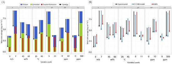
Figure 13.
Synergy of wear modes: (A) contribution to erosion, corrosion, and synergy in the experimental data. Synergy is represented by an arrow with downward direction corresponding to negative synergy, (B) and comparison of synergy contribution to E-C wear rate as measured (black arrows) and as predicted by the E-C NN.
All the tendencies observed in the experimental data are also present in the E-C NN predictions, which is not always the case for the MFA predictions, as shown in Figure 13B. In particular, the negative sign of synergy is incorrectly predicted for a high level of (11) and low level of (0 ppm). This difference might not be significant, however, when considering that the value is comparable with experimental error. In this study, only main effects are discussed. In order to explain the origin of the synergy, cross-correlations would have to be examined, but such an analysis is beyond the scope of the present study.
Figure 13 shows that velocity plays a significant role in the wear rate, both in stand-alone erosion and corrosion, as well as in the combined E-C mechanism. The V parameter derives from the flow field, which due to it inherent turbulence, affects the kinetic energy conveyed by the particles and also the convection-diffusion mass transfer for corrosion wear. Notably, the impact of particle concentration was not clearly distinguished between the stand-alone erosion and corrosion experiments. This observation can be associated with the fact that particle concentration changes fluid viscosity, consequently influencing the Reynolds number of the system [45], which in turn governs turbulence. Flow-induced corrosion is a critical mechanism in such systems, and this effect was not fully captured by these experiments, leading to a biased interpretation of the particle concentration effect. However, it could explain the negative synergy observed, primarily reducing the corrosion effect. In contrast, the corrosion experiment conducted without particles experienced reduced fluid viscosity, which resulted in augmented flow-induced corrosion and an increase in the corrosion wear rate [46]. In the other experiments, the presence of particles increased fluid viscosity [47,48], leading to a reduction in the Reynolds number (Turbulence level) and, consequently, the corrosion wear rate [46].
The above discussion of synergy shows the importance of correctly modeling the relative contributions of stand-alone effects as they are associated with physical processes that might be studied by analysis of microstructure. However, the high cost of microstructural analysis over the extended design of the experiment can be diminished by the use of E-C NN, as shown in Figure 13B in which superior capacity of the ANN to predict synergy is compared with that of the MFA.
Finally, this research is considered to provide a “toolbox” for effectively predicting E-C wear and understanding its underlying mechanisms. The results emphasize the superiority of ANN over regression models in E-C analysis, offering new alternatives for improving wear prediction accuracy and informing engineering practices aimed at mitigating wear in various systems and applications.
5. Conclusions
In this work, applicability of artificial neural networks (ANN) for predicting E-C wear was explored in comparison to the conventional regression models based on MFA. Previously published experimental data on E-C rate were complemented with new data on stand-alone erosion and stand-alone corrosion. The effect of pre-training was verified with the general conclusion that the pre-trained and fine-tuned ANN outperforms the regression models in accurately predicting the wear rates, indicating that the flexibility of ANN is better suited to represent the complex relationships and patterns that may be omitted by the conventional MFA models. In particular:
- -
- Combination of experimental data with synthetic data generated by the MFA model provides a larger and more diverse dataset, enhancing the training process and improving the generalisation of the applicability and the capabilities of the ANN model in the specific field of E-C studies.
- -
- The ANN shows a superior performance compared to the MFA counterpart as assessed by the mean and median squared errors (MSE). The performance is further improved by including a pre-training step, reducing the mean and median MSE from 3.623 to 2.535, and 0.019 to 0.005, respectively, as compared with 3.694 and 0.345, respectively, of the MFA.
- -
- The ANN trained on E-C data, i.e., the E-C NN, is capable of generalising the importance of experimental parameters without overemphasizing noise in the data, as shown by the absence of global overfitting.
- -
- The errors of the E-C NN predictions are consistently lower than the stand-alone experimental errors, indicating that the model provides highly confident predictions within the factor ranges, outperforming the predictions obtained using MFA.
- -
- Velocity emerges as the predominant factor across all wear mechanisms studied in this work, underscoring the necessity for future focused and deterministic investigations on the specific impact of this parameter in each wear mechanism.
- -
- The synergy effect is highly pronounced compared to the stand-alone wear rate impact. Conducting a detailed study to thoroughly understand and model this particular effect, as well as identifying the key factors that significantly influence it, is of paramount importance.
- -
- Exploring the genuine impact of particle concentration and its influence on fluid viscosity in corrosion wear becomes crucial for a comprehensive understanding of corrosion and E-C wear mechanisms.
In conclusion, the E-C NN proves to be a superior method for predicting wear rates, owing to its comprehensive consideration of all factors and their effects, including direct and synergistic effects. On the other hand, MFA’s exclusion of certain parameters to improve linear regression fit limits its ability to fully represent the complexity of erosion-corrosion phenomena. The E-C NN delivers more accurate and reliable predictions, establishing itself as a robust tool for exploring E-C behaviour and advancing tribological research. Moreover, the computational cost of training the ANN model is reasonable, making it viable even with small datasets. This advantage allows for the practical implementation of ANN models in E-C wear analysis, even under data constraints or limited computational resources. As a result, the E-C NN emerges as a promising approach with wide-ranging applications, enabling researchers to gain deeper insights into erosion-corrosion processes and pave the way for future advancements in the field.
Author Contributions
Conceptualisation, M.W. and A.E.-J.; Experiment, J.A.; Software, A.E.-J.; Formal analysis, A.E.-J., I.W. and M.W.; Investigation, A.E.-J. and M.W.; Resources, M.W.; Data curation, A.E.-J.; Writing—original draft preparation, A.E.-J.; writing—review and editing, A.E.-J., M.W. and I.W.; Visualisation, A.E.-J. and M.W.; Supervision, M.W.; Project administration and funding acquisition, M.W. All authors have read and agreed to the published version of the manuscript.
Funding
This research was funded by ANID (Agencia Nacional de Investigación y Desarrollo de Chile) through the grant FONDECYT Regular 1201547 and Pontificia Universidad Católica de Chile through the scholarship Beca VRI.
Institutional Review Board Statement
Not applicable.
Data Availability Statement
The data presented in this study combine results published by Aguirre et al. [35] with new data. The entire set of experimental data is provided as Appendix A.
Acknowledgments
The authors convey special thanks to Alvaro Soto for the inspiration to apply machine learning to the exotic field of E-C and to Alejandro Mac Cawley for his advice in conducting the statistical analysis.
Conflicts of Interest
The authors declare no conflict of interest.
Abbreviations
The following abbreviations are used in this manuscript:
| ANN | Artificial neural network |
| E-C NN | Erosion-corrosion neural network |
| MFA | Multifactorial analysis |
| MSE | Meas squared error |
| RSM | Response surface method |
Appendix A
Data of weight loss in mg·cmh measured in all the experimental runs.

Table A1.
Erosion data.

Table A2.
Corrosion data.

Table A3.
Erosion-Corrosion data.
References
- Moore, P. Ausenco Symposium Outlines Importance of Long Term Mining Slurry Pipeline Management; Ausenco: South Brisbane, Australia, 2018. [Google Scholar]
- ASTM G119-09; Standard Guide for Determining Synergism Between Wear and Corrosion. ASTM International: West Conshohocken, PA, USA, 2021. [CrossRef]
- Javaheri, V.; Porter, D.; Kuokkala, V.T. Slurry erosion of steel—Review of tests, mechanisms and materials. Wear 2018, 408, 248–273. [Google Scholar] [CrossRef]
- Turenne, S.; Fiset, M.; Masounave, J. The effect of sand concentration on the erosion of materials by a slurry jet. Wear 1989, 133, 95–106. [Google Scholar] [CrossRef]
- Neville, A.; Hodgkiess, T.; Xu, H. An electrochemical and microstructural assessment of erosion–corrosion of cast iron. Wear 1999, 233, 523–534. [Google Scholar] [CrossRef]
- Stachowiak, G.W. Particle angularity and its relationship to abrasive and erosive wear. Wear 2000, 241, 214–219. [Google Scholar] [CrossRef]
- Stack, M.; Jana, B. Modelling particulate erosion–corrosion in aqueous slurries: Some views on the construction of erosion–corrosion maps for a range of pure metals. Wear 2004, 256, 986–1004. [Google Scholar] [CrossRef]
- Desale, G.R.; Gandhi, B.K.; Jain, S. Effect of erodent properties on erosion wear of ductile type materials. Wear 2006, 261, 914–921. [Google Scholar] [CrossRef]
- Tian, B.R.; Cheng, Y.F. Electrochemical corrosion behavior of X-65 steel in the simulated oil sand slurry. I: Effects of hydrodynamic condition. Corros. Sci. 2008, 50, 773–779. [Google Scholar] [CrossRef]
- Rauf, A.; Mahdi, E. Studying and comparing the erosion-enhanced pitting corrosion of X52 and X100 steels. Int. J. Electrochem. Sci. 2012, 7, 5692–5707. [Google Scholar] [CrossRef]
- Wood, R.J.K.; Walker, J.C.; Harvey, T.J.; Wang, S.; Rajahram, S.S. Influence of microstructure on the erosion and erosion–corrosion characteristics of 316 stainless steel. Wear 2013, 306, 254–262. [Google Scholar] [CrossRef]
- Islam, A.M.; Farhat, Z.N.; Ahmed, E.M.; Alfantazi, A.M. Erosion enhanced corrosion and corrosion enhanced erosion of API X-70 pipeline steel. Wear 2013, 302, 1592–1601. [Google Scholar] [CrossRef]
- Yu, B.; Li, D.Y.; Grondin, A. Effects of the dissolved oxygen and slurry velocity on erosion-corrosion of carbon steel in aqueous slurries with carbon dioxide and silica sand. Wear 2013, 302, 1609–1614. [Google Scholar] [CrossRef]
- Lindgren, M.; Perolainen, J. Slurry pot investigation of the influence of erodent characteristics on the erosion resistance of austenitic and duplex stainless steel grades. Wear 2014, 319, 38–48. [Google Scholar] [CrossRef]
- Malik, J.; Toor, I.; Ahmed, W.; Gasem, Z.; Habib, M.; Ben-Mansour, R.; Badr, H. Investigations on the Corrosion-Enhanced Erosion Behavior of Carbon Steel AISI 1020. Int. J. Electrochem. Sci. 2014, 9, 6765–6780. [Google Scholar] [CrossRef]
- Islam, M.A.; Alam, T.; Farhat, Z.N.; Mohamed, A.; Alfantazi, A. Effect of microstructure on the erosion behavior of carbon steel. Wear 2015, 332, 1080–1089. [Google Scholar] [CrossRef]
- Zheng, Z.; Zheng, Y. Erosion-enhanced corrosion of stainless steel and carbon steel measured electrochemically under liquid and slurry impingement. Corros. Sci. 2016, 102, 259–268. [Google Scholar] [CrossRef]
- Jiang, J.; Xie, Y.; Islam, A. The Effect of Dissolved Oxygen in Slurry on Erosion–Corrosion of En30B Steel. J. Bio Tribo-Corros. 2017, 3, 45. [Google Scholar] [CrossRef]
- Kuruvila, R.; Kumaran, S.T.; Khan, M.A.; Uthayakumar, M. A brief review on the erosion-corrosion behavior of engineering materials. Corros. Rev. 2018, 36, 435–447. [Google Scholar] [CrossRef]
- Yi, J.Z.; Hu, H.X.; Wang, Z.B.; Zheng, Y.G. On the critical flow velocity for erosion-corrosion in local eroded regions under liquid-solid jet impingement. Wear 2019, 423, 94–99. [Google Scholar] [CrossRef]
- Messa, G.V.; Wang, Y.; Malavasi, S. A discussion of the test procedures of the API 6AV1 standard based on wear prediction simulations. Wear 2019, 426, 1416–1429. [Google Scholar] [CrossRef]
- Nicholls, J.R.; Stephenson, D.J. Monte Carlo modelling of erosion processes. Wear 1995, 186, 64–77. [Google Scholar] [CrossRef]
- Haider, G.; Arabnejad, H.; Shirazi, S.A.; Mclaury, B.S. A mechanistic model for stochastic rebound of solid particles with application to erosion predictions. Wear 2017, 376, 615–624. [Google Scholar] [CrossRef]
- Das, S.K. Application of a Stochastic Modelling Framework to Characterize the Influence of Different Oxide Scales on the Solid Particle Erosion Behaviour of Boiler Grade Steel; Technical Report; Indian Academy of Sciences: Karnataka, India, 2011. [Google Scholar]
- de Moura, B.F.; da Silva, W.B.; de Macêdo, M.C.S.; Martins, M.F. A statistical approach to estimate state variables in flow-accelerated corrosion problems. Inverse Probl. Sci. Eng. 2018, 26, 966–995. [Google Scholar] [CrossRef]
- Vencl, A.; Svoboda, P.; Klančnik, S.; But, A.; Vorkapić, M.; Harničárová, M.; Stojanović, B. Influence of Al2O3 Nanoparticles Addition in ZA-27 Alloy-Based Nanocomposites and Soft Computing Prediction. Lubricants 2023, 11, 24. [Google Scholar] [CrossRef]
- Lalwani, V.; Sharma, P.; Pruncu, C.I.; Unune, D.R. Response surface methodology and artificial neural network-based models for predicting performance of wire electrical discharge machining of inconel 718 alloy. J. Manuf. Mater. Process. 2020, 4, 44. [Google Scholar] [CrossRef]
- Ibrahim, S.; Abdul Wahab, N. Improved Artificial Neural Network Training Based on Response Surface Methodology for Membrane Flux Prediction. Membranes 2022, 12, 726. [Google Scholar] [CrossRef] [PubMed]
- Oh, S. Comparison of a response surface method and artificial neural network in predicting the aerodynamic performance of a wind turbine airfoil and its optimization. Appl. Sci. 2020, 10, 6277. [Google Scholar] [CrossRef]
- Patel, K.A.; Brahmbhatt, P.K. A Comparative Study of the RSM and ANN Models for Predicting Surface Roughness in Roller Burnishing. Procedia Technol. 2016, 23, 391–397. [Google Scholar] [CrossRef]
- Abiodun, O.I.; Kiru, M.U.; Jantan, A.; Omolara, A.E.; Dada, K.V.; Umar, A.M.; Linus, O.U.; Arshad, H.; Kazaure, A.A.; Gana, U. Comprehensive Review of Artificial Neural Network Applications to Pattern Recognition. IEEE Access 2019, 7, 158820–158846. [Google Scholar] [CrossRef]
- Hasan, M.S.; Nosonovsky, M. Triboinformatics: Machine learning algorithms and data topology methods for tribology. Surf. Innov. 2022, 10, 229–242. [Google Scholar] [CrossRef]
- Kokol, P.; Kokol, M.; Zagoranski, S. Machine learning on small size samples: A synthetic knowledge synthesis. Sci. Prog. 2022, 105, 003685042110297. [Google Scholar] [CrossRef]
- Barrionuevo, G.O.; Walczak, M.; Ramos-Grez, J.; Sánchez-Sánchez, X. Microhardness and wear resistance in materials manufactured by laser powder bed fusion: Machine learning approach for property prediction. CIRP J. Manuf. Sci. Technol. 2023, 43, 106–114. [Google Scholar] [CrossRef]
- Aguirre, J.; Walczak, M. Multifactorial study of erosion–corrosion wear of a X65 steel by slurry of simulated copper tailing. Tribol. Int. 2018, 126, 177–185. [Google Scholar] [CrossRef]
- ASTM G1-03 (Reapproved 2017); Standard Practice for Preparing, Cleaning, and Evaluating Corrosion Test. ASTM International: West Conshohocken, PA, USA, 2017.
- R Core Team. A Language and Environment for Statistical Computing; R Core Team: Vienna, Austria, 2022. [Google Scholar]
- Ulrike Groemping. FrF2: Fractional Factorial Designs with 2-Level Factors; Ulrike Groemping: Berlin, Germany, 2023. [Google Scholar]
- Lumley, T.; Miller, A. leaps: Regression Subset Selection. 2023. Available online: https://cran.r-project.org/web/packages/leaps/leaps.pdf (accessed on 1 October 2022).
- Kobayashi, M.; Sakata, S. Mallows’ C criterion and unbiasedness of model selection. J. Econom. 1990, 45, 385–395. [Google Scholar] [CrossRef]
- Keyes, T.K.; Levy, M.S. Goodness of Prediction Fit for Multivariate Linear Models. J. Am. Stat. Assoc. 1996, 91, 191–197. [Google Scholar] [CrossRef]
- Pedregosa, F.; Varoquaux, G.; Gramfort, A.; Michel, V.; Thirion, B.; Grisel, O.; Blondel, M.; Prettenhofer, P.; Weiss, R.; Dubourg, V.; et al. Scikit-learn: Machine Learning in Python. J. Mach. Learn. Res. 2011, 12, 2825–2830. [Google Scholar]
- Aguirre, J.; Walczak, M.; Rohwerder, M. The mechanism of erosion-corrosion of API X65 steel under turbulent slurry flow: Effect of nominal flow velocity and oxygen content. Wear 2019, 438, 203053. [Google Scholar] [CrossRef]
- Clark, H.M. Particle velocity and size effects in laboratory slurry erosion measurements OR... do you know what your particles are doing? Tribol. Int. 2002, 35, 617–624. [Google Scholar] [CrossRef]
- Grossmann, S.; Lohse, D.; Sun, C. High–Reynolds Number Taylor-Couette Turbulence. Annu. Rev. Fluid Mech. 2016, 48, 53–80. [Google Scholar] [CrossRef]
- Fang, C.S.; Liu, B. Hydrodynamic and temperature effects on the flow-induced local corrosion rate in pipelines. Chem. Eng. Commun. 2003, 190, 1249–1266. [Google Scholar] [CrossRef]
- Stickel, J.J.; Powell, R.L. Fluid mechanics and rheology of dense suspensions. Annu. Rev. Fluid Mech. 2005, 37, 129–149. [Google Scholar] [CrossRef]
- Chen, S.H.; Li, X.F. Effects of particle concentration and physical properties on the apparent viscosity of a suspension of monodisperse concentric core–shell particles. Eur. J. Mech. B/Fluids 2020, 84, 542–552. [Google Scholar] [CrossRef]
Disclaimer/Publisher’s Note: The statements, opinions and data contained in all publications are solely those of the individual author(s) and contributor(s) and not of MDPI and/or the editor(s). MDPI and/or the editor(s) disclaim responsibility for any injury to people or property resulting from any ideas, methods, instructions or products referred to in the content. |
© 2023 by the authors. Licensee MDPI, Basel, Switzerland. This article is an open access article distributed under the terms and conditions of the Creative Commons Attribution (CC BY) license (https://creativecommons.org/licenses/by/4.0/).

