Investigation of Programmable Friction with Ionic Liquid Mixtures at the Nano- and Macroscales

Abstract

Non-mechanical stimuli are used to directly control or program the friction properties of tribosystems. For this purpose, an ionic liquid is used as a lubricant that affects and controls the friction in the presence of external triggers. Here, it is shown that the friction behavior of two surfaces in sliding contact can be controlled and permanently changed by applying an electrical potential to an ionic liquid mixture (ILM). This change in the friction properties was demonstrated both at the nanoscale using an atomic force microscopy (AFM)-based friction force microscopy (FFM) and at the macroscale using a specially designed tribo-setup cell. In tribology, the linking of these two scales of magnitude represents one of the greatest obstacles between basic research and the step towards application-oriented system development and is therefore of fundamental importance. In addition, other parameters affecting the tribological behavior of the system, such as roughness, lubricant film thickness, and wear behavior, were investigated as a function of the electrical potentials. The correlation between the structure of surface-bound ionic liquid layers and the friction behavior can be used to control friction, thus enabling a first step towards tribosystems that automatically adapt to changing conditions.

1. Introduction

Friction and wear occur in all objects in mechanical contact under relative motion and cause enormous ecological and economic costs. Friction contributes significantly to global energy consumption, and thus also increases carbon dioxide emissions [1]. Therefore, tribological research is investigating new surfaces (coatings such as diamond-like carbon coatings and structures), materials (including self-lubrication), and lubricants to reduce friction and wear in mechanically stressed components [2]. Due to the global challenges regarding environmental protection and energy efficiency, the focus of tribological research is currently on sustainable lubrication. Environmentally compatible and superlubricating systems are investigated to improve the efficiency and reliability of machines. In this context, superlubricity [3,4], bioinspired polymers [5], biolubricants [6], sustainable lubricants [7], ionic liquids (ILs) [8], ILs as additives to bio lubricants [9], aqueous lubricants [10], and electrotunable systems [11] are relevant research topics. The energy saving for the environment in a tribological system consists not only of the use of sustainable raw materials, but also in the use of coordinated and perfectly matching lubricant components that bring savings in friction and wear due to their properties and thus protect the environment. With the increasing power density in tribological applications and the use of electrified systems, the functional requirements for lubrication systems are also increasing [12]. Therefore, new tribological concepts, such as programmable friction, need to be developed to meet the increasing demands.

The state of the art in developing lubricants for a particular application is to optimize them for the full range of operating parameters. Due to different properties of the lubricants (including viscosity, stability, chemical interactions), ideal lubrication conditions cannot be realized at all operating conditions [13]. Therefore, a compromise must always be made in the technical design and lubricant composition. In addition, due to aging and wear, the optimal operating point of a machine may move further away from the friction optimum during its lifetime. One solution to this problem is the development of systems whose tribological properties can be changed by an external stimulus. Especially attractive are systems where an electric stimulus is used (potential controlled friction (PCF) [14], tribotronics [15]). Programmable friction is the targeted control of friction through additional integrated condition monitoring systems and computer-controlled coefficient of friction (COF) adjustment in a tribological system [16]. This is intended to optimize the lubrication properties continuously and at every operating point over the entire running time. Program-controlled adaptation to operating conditions can lead to increased energy efficiency and service life of tribological systems. In the last 20 years, several publications have reported that the friction of metal–metal and metal–ceramic contacts in surfactant-containing solutions can be actively influenced by the application of electrical voltages [17]. Electrically tunable friction with ionic liquid lubricants has been intensively investigated [11,18]. By tuning the friction through applied potentials, there isthe possibility of programming the friction via feedback control of the electrical resistance in the tribological contact [19]. By applying a voltage to a tribological contact lubricated with an IL, the COF can be controlled in real time and ultra-low friction can be achieved. This tribological behavior is caused by the strong interactions between the ionic layers and the surfaces, which prevent the liquid from “squeezing out”, leading to lubricant deprivation and wear under pressure [11,20]. As a result, robust lubrication can be achieved. Lubrication with ILs takes advantage of two key properties. The ions are tightly bound to the surfaces by their electrostatic interactions, but the film remains fluid up to a certain pressure [21,22]. The relationship between the voltage effect on the structure of surface-bound IL layers and their lubricating properties is determined by the surface charge and the resulting exchange of anion or cation layers on the surfaces [20]. These layers provide an important path to good boundary lubrication, which occurs in only a few other scenarios, such as hydration lubrication [23]. The main effect of adsorption and layer blending of IL molecules on the surface is thought to be an increase of the anisotropy of the viscosity [24]. The different degrees of adsorption of cations (weak) and anions (strong) lead to differences in the lubricant film thickness. Polar carboxyl groups on the anion can serve as anchors for the formation of a strongly adsorbed ion film. Electrical potential enhances the adsorption of ions at the interface, resulting in changes in relative cation/anion density [25].

Table 1 lists tribosystems and the maximum changes in the COF obtained by applying an external voltage (Figure S1). In these publications, different COF changes were measured at different electrical potentials. The electrotribological investigations were carried out with different material pairs, lubricants, and load collectives. Therefore, the values of the friction properties are rather difficult to compare with each other. With two exceptions, the results are listed for lubrication with ILs. With pure IL, a maximum COF reduction between application of a high and low potential of about 95% is achieved in a nanoscale contact. In addition, using atomic force microscopy (AFM), superlubricity was measured with an electrical potential applied to an IL [26]. With an IL–oil mixture, a maximum COF change of 125% at 3 V was achieved macroscopically [24]. The maximum COF change, in the publications considered, of 170% was obtained using sodium dodecyl sulfate (SDS) aqueous solution at −2 V [27].

In our own research work, the influence of electrical potentials on the wear behavior of steel under cavitation could be observed [28,29]. The friction behavior could be influenced by electrical potentials under water lubrication with ceramics [30,31] and in aqueous mixtures with ILs [32]. A change in COF with steel was also demonstrated with pure ILs [33,34]. Programmable friction by computer-controlled realization of preset COF could be achieved by using ionic liquid mixtures (ILMs) together with a tribo-controller that autonomously regulates the electrical potential [16,35]. It was found that with ILMs, the COF can be influenced significantly more than with pure ILs. In addition, it was demonstrated that the surface charge has a stronger effect on the COF change at lower film thicknesses. This agrees well with simulation results because the structure formation of the IL extends over only a few layers. If the lubricant film is too thick (hydrodynamic friction condition), IL adsorption no longer has any influence on the friction behavior. However, it is still unknown as to how the COF can be changed more strongly with the use of ILMs than with pure ILs at the same electrical potentials. The electrotribology of ILMs has been investigated by Gatti et al. [16]. As the electrotribology of pure ILs has been intensively studied through simulation [20,22,36,37] and analytical methods [38,39], the mechanisms involved in pure ILs are already well described. Therefore, the current model of the mechanism of the tribocontrol of ILMs is based on the interactions of pure ILs. The ions are adsorbed on the surface to different extents depending on the surface charge and chemical structure of the ions, resulting in layer formation on the respective surface. This adsorption causes an increase in viscosity and a change in lubricant film thickness, which alters the COF. As a larger COF change can be achieved with ILMs than with pure ILs, the interaction of the ions with the charged surface must increase in the presence of two anions. However, the adsorption and structure formation of ions on a surface depend not only on the chemical structure of the ions and the charge density, but also on the purity of the ILs. The structure formation of ILs can be influenced by the addition of alkanol mixtures [40]. Steric effects act between the IL and the alkanols, and self- and heteroaggregation by hydrogen bonding occurs. These two factors lead to contractive mixing and strong hydrogen bonding between IL and alkanol. In the presence of water, applying a voltage can increase friction, because the polar water molecules are attracted by the electric field and accumulate around the friction body [41]. The COF for a single bilayer of an IL is independent of water content, while for two bilayers it increases by more than an order of magnitude when water is added. This effect is due to the increase in the order of the ions within the shear plane [41,42,43,44].

COF changes were more pronounced for ILMs than for pure ILs in the electrotribological contact. This difference can be explained by the following hypothesis: ILMs form denser and tribologically more stable adsorption layers in the electric field than pure ILs. In order to test this hypothesis and to reveal the involved mechanisms for ILMs in the electrotribological contact, nano- and macroscale electrotribological friction experiments were performed. The aim was not to adjust the friction to a desired value during a tribological experiment, but to show that the COF can be actively changed or switched with an external potential compared to a COF that adjusts without a potential in a tribological experiment. Therefore, only constant electrical potentials were used in this work. To show the variability of the COF under different friction regimes, multi-experiments were performed, which included the characterization of static and sliding friction, and then Stribeck curves were then generated, while in previous works the focus was on the changeability and programmability of COF(Figure S2) [16].

To evaluate the effects of impurities in the ILs and the consequent presumed change in tribological properties due to an electric field, water and ethanol were added to the ILMs. To find out which chemical reactions take place when the electrochemical load is too high or whether the two individual IL components had already reacted with each other during mixing, tests were made with nuclear magnetic resonance spectroscopy (NMR). As the influence of the lubricant film thickness on the COF change has been demonstrated by electrical potentials in our preliminary work, high-pressure rheology was performed to calculate the lubricant film thickness according to Hamrock and Dowson. The overall aim of this work was to create interfaces between nano- and macrotribology regarding the changeability of COF with external electrical potentials using ILMs in order to improve tribological properties and possibly create tribological systems for technical applications in the future, saving energy and resources and thus protecting the environment.

Table 1. Literature values on the influence of the COF by externally applied electrical potentials.

Reference	Geometry	Material	Lubricant	el. Potential	Change in COF *
				V	-	%
Gat 2019 [35]	ball-on-3-pins	100Cr6	[P66614][DEHP]:[P66614][BTA] 1:3	3.0	0.028	26.7
			“	−3.0	−0.005	−4.8
Gat 2020 [16]	ball-on-3-pins	100Cr6	[P66614][Doc]:[P66614][BTA] 1:4	3.0	0.045	45.0
			“	−3.0	−0.004	−4.3
Kaw 2019 [45]	disk-on-disk	AISI 52100 + ta-C	[BMIM][FAB]	4.0	0.027	40.9
			[BMIM][PF6]	−2.0	−0.004	−6.3
Guo 2019 [46]	ball-on-disk	GCr15	C10 NFs	4.5	−0.017	−13.5
Mic 2020 [47]	ball-on-disk	C45/C10	[BMIM]PF6	1.0	0.023	69.2
Li 2014 [26]	AFM cantilever tip on plate	Si/HOPG	[HMIm]FAP	−1.0	0.001	5.3
			“	1.5	−0.018	−94.7
Yang 2014 [48]	ball-on-disk	ZrO2/steel 4340	PC oil	0.6	0.020	8.0
			[DMIm]PF6/PC (0.5 mM)	−0.6	−0.120	−46.2
Zhang 2022 [24]	ball-on-disk	GCr15	1 wt.% [OMIm]PF6 + PAO50	3.0	0.100	125.0
Liu 2021 [27]	ball-on-disk	ZrO2/Al2O3	1 mM SDS and 10 mM NaCl	−2.0	0.220	169.2

* The stated change in COF could deviate slightly from the measured values since most of the values were read from diagrams.

Table 1. Literature values on the influence of the COF by externally applied electrical potentials.

Reference	Geometry	Material	Lubricant	el. Potential	Change in COF *
				V	-	%
Gat 2019 [35]	ball-on-3-pins	100Cr6	[P66614][DEHP]:[P66614][BTA] 1:3	3.0	0.028	26.7
			“	−3.0	−0.005	−4.8
Gat 2020 [16]	ball-on-3-pins	100Cr6	[P66614][Doc]:[P66614][BTA] 1:4	3.0	0.045	45.0
			“	−3.0	−0.004	−4.3
Kaw 2019 [45]	disk-on-disk	AISI 52100 + ta-C	[BMIM][FAB]	4.0	0.027	40.9
			[BMIM][PF6]	−2.0	−0.004	−6.3
Guo 2019 [46]	ball-on-disk	GCr15	C10 NFs	4.5	−0.017	−13.5
Mic 2020 [47]	ball-on-disk	C45/C10	[BMIM]PF6	1.0	0.023	69.2
Li 2014 [26]	AFM cantilever tip on plate	Si/HOPG	[HMIm]FAP	−1.0	0.001	5.3
			“	1.5	−0.018	−94.7
Yang 2014 [48]	ball-on-disk	ZrO2/steel 4340	PC oil	0.6	0.020	8.0
			[DMIm]PF6/PC (0.5 mM)	−0.6	−0.120	−46.2
Zhang 2022 [24]	ball-on-disk	GCr15	1 wt.% [OMIm]PF6 + PAO50	3.0	0.100	125.0
Liu 2021 [27]	ball-on-disk	ZrO2/Al2O3	1 mM SDS and 10 mM NaCl	−2.0	0.220	169.2

* The stated change in COF could deviate slightly from the measured values since most of the values were read from diagrams.

2. Materials and Methods

2.1. Materials and Used Ionic Liquids

The ILs used in this study were trihexyltetradecylphosphonium-bis(trifluoromethylsulfonyl)-imide [P66614][BTA] (IN-0021, IoLiTec Ionic Liquids Technologies GmbH, Heilbronn, BW, Germany, η: 310 mPa·s at 25 °C, 2400 ppm water, κ: 140 µS/cm at 30 °C, M: 763.2 g/mol, chemical structure: see Figure S3) and trihexyltetradecylphosphonium docusate [P66614][Doc] (CS-0641, IoLiTec Ionic Liquids Technologies GmbH, Heilbronn, BW, Germany, η: 1392 mPa·s at 25 °C, 973 ppm water, κ: 0.05 µS/cm at 25 °C, M: 905.4 g/mol, chemical structure: see Figure S3). These two ILs were mixed in a mass ratio of [BTA] to [Doc] 4:1. The ILs were stored in a glovebox under nitrogen atmosphere to keep the water content of the ILs constant. In addition, this ILM of the two ionic liquids was mixed with 10% water or 10% ethanol and tribologically tested.

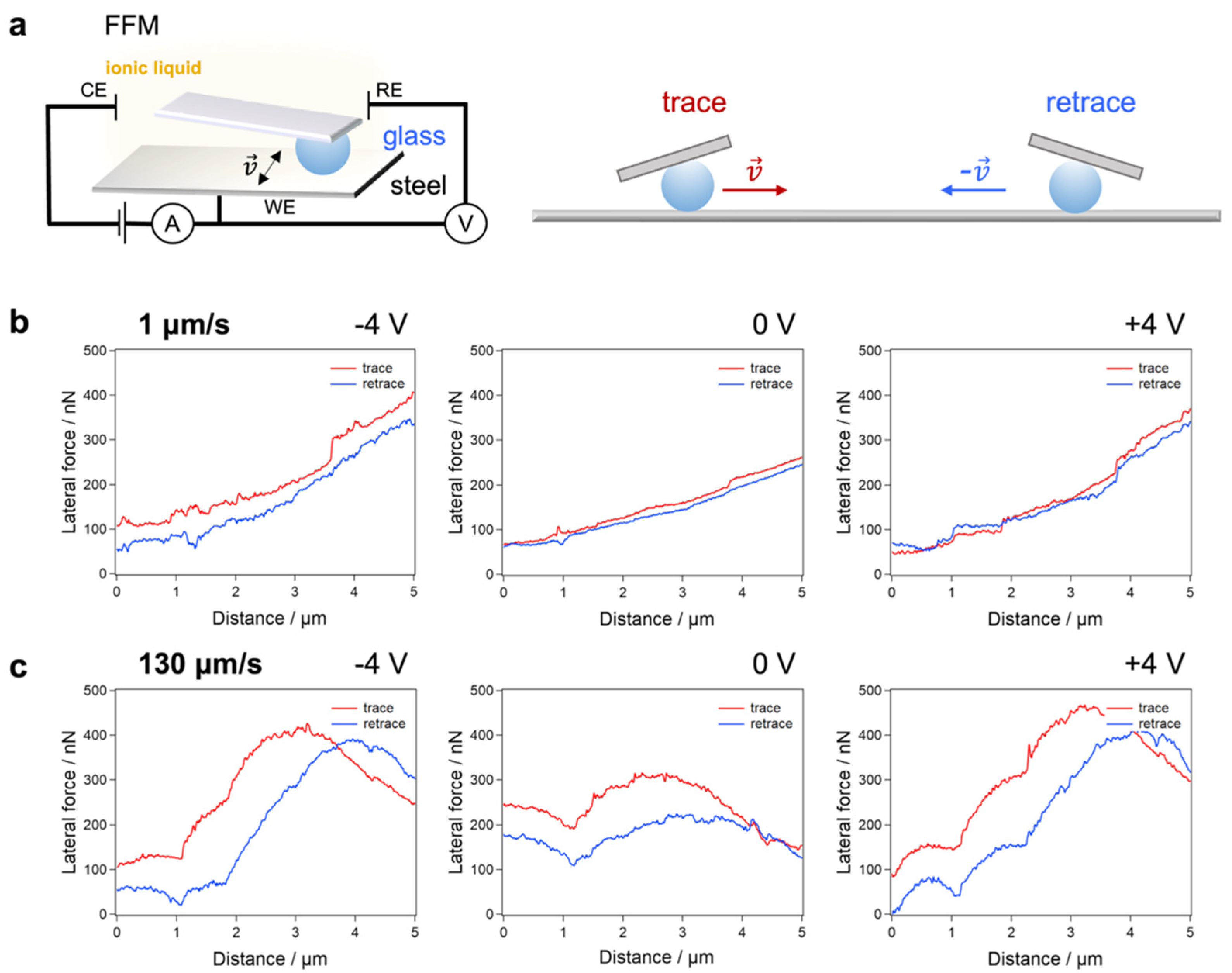
2.2. Friction Force Microscopy Experiments

Atomic force microscopy (AFM)-based friction force microscopy (FFM) experiments between a borosilicate glass bead and a steel sample (pin, 100Cr6, 750-850 HV10, Ra = 0.32 (±0.05) µm, Rz = 2.47 (±0.29) µm) were carried out on a Cypher ES (Asylum Research, an Oxford Instruments Company, Santa Barbara, CA, USA) in ILM at approximately 25 °C. To do so, an AFM cantilever carrying a borosilicate glass bead with a diameter size of 10 μm (Novascan Technologies, Boone, IA, USA) was used. Prior to the experiments, the vertical spring constant (approx. 1–2 N/m) of the cantilever was calibrated using the Sader method (130 μm length, 35 μm width, 150 kHz resonance frequency) in the GetReal panel for automated calibration of a custom rectangular lever in air; the lateral sensitivity of the cantilever (approximately 4 μN/V) was calibrated using a diamagnetic levitation force calibrator (DLFC) in air prior to the FFM experiment [49,50]. Prior to use in experiments, the steel pins were sonicated in ethanol (>99.95%, VWR, Rosny-sous-Bois, France) for 30 min (Elmasonic S15, Elma, Singen, Germany). An electrochemical cell (EC cell) for the Cypher ES was used. In the EC cell, the steel pin was contacted to a Cu working electrode (WE) using silver paint 200 (Ted Pella, Redding, CA, USA); the counter electrode (CE) was Pt and the reference electrode (RE) was an Ag wire positioned close to the cantilever chip (three-electrode setup). The electrical potentials were applied via a potentiostat (630 E, CH Instruments, Austin, TX, USA). A voltammogram was taken to verify the proper functioning of the EC cell (Figure S4).

In order to verify the quality of glass bead gluing to AFM cantilevers, exemplary cantilevers were investigated by scanning electron microscopy (SEM, FEI Quanta 250 FEG, Oxford Instruments, Abingdon, UK) in low vacuum mode (113 Pa; water atmosphere) at an accelerating voltage of 10.00 kV using a large field detector (Figure S5a). Different normal forces F_N (649–3245 nN) and scan velocities v (1–130 μm/s) were used for the FFM experiments, while for each F_N, different v was measured in a row from the lowest 1 μm/s to the highest 130 μm/s. For each of the experimental conditions, the FFM experiments were carried along the same single line (slow scan disabled) having a length of 5 μm for at least 64 times. There, the fast scan axis was perpendicular to the cantilever axis. As a control experiment, the FFM experiments were also carried out in bulk ILM, in which the cantilever was moved far away from the steel surface and the measured friction was only due to the viscous friction of the liquid. For all the FFM experiments, the friction force F_R was calculated from the friction loop (trace and retrace curves) via Equation (1) [51,52,53].

$$F_R=\frac{F_{trace}-F_{retrace}}{2}$$

(1)

To estimate the adhesion between the glass bead and the steel surface, the adhesive forces at different normal forces (trigger forces) F_N and electrical potentials were obtained from the vertical force–extension curves by retracting the AFM cantilever tip from the surface at a velocity of 1 μm/s (Figure S5). For each experimental condition, at least 10 curves were collected for this estimation.

2.3. AFM-Based Imaging

AFM-based imaging of the steel pins was performed on a Cypher ES (Asylum Research, an Oxford Instruments Company, Santa Barbara, CA, USA) using the intermittent-contact mode (AC mode) with photothermal excitation (blueDrive) at 25 °C in air with AC240TS cantilevers (Olympus, Japan, spring constant: 2 N/m, resonance frequency: 70 kHz, tip radius: approximately 7 nm). AFM imaging of steel balls was performed on a XE7 (Park Systems, Suwon, Republic of Korea) using the intermittent-contact mode (tapping mode) with mechanical excitation at approximately 22 °C in air with SCOUT 70 RAl cantilevers (NuNano, Bristol, UK, spring constant: 2 N/m, resonance frequency: 70 kHz, tip radius: approximately 5 nm). Further imaging parameters were the pixel number: 512·512, the scan rate: 1 Hz and the scan angle: 0° (Cypher ES) and 90° (XE7), i.e., fast scan axis was parallel to the cantilever axis. The samples were glued on mounting pucks using High Resolution Replicating Compound 101RF (Microset Products, Hinckley, UK) and then treated with a mild stream of N₂ for a few seconds prior to imaging to remove any sample debris that might interfere with the AFM imaging process.

For evaluation, the images were processed with the Gwyddion Free SPM analysis software version 2.60 [54] using the following operations in the presented order: mean plane subtraction, line median matching (median of differences), correction of horizontal scars, and shifting of minimum data values to zero (fix zero function). A linear color scale, gwyddion.net, was used for the presentation of the images. Afterwards, the root mean square (RMS) roughness and line profiles were extracted.

2.4. Viscosity and Pressure–Viscosity Coefficient

The MCR501 rheometer (Anton Paar, Graz, Austria) with rotating plate geometry (diameter: 50 mm) was used to measure the viscosity of the lubricants. Viscosity was measured while passing through a temperature ramp from 0 °C to 50 °C (temperature rise: 2 °C/min) at a constant shear rate (50 s⁻¹). The pressure–viscosity coefficient (α) of the ILM was measured using a high-pressure cell (double-slit Searle measuring principle for MCR 501). In this process, a hollow cylinder was rotating in a stable cup in which a second fixed cylinder was stationary concentrically to the axis of rotation. The inner gap was 0.4 mm, and the outer gap was 0.44 mm. The amount of liquid used was 8 mL. Viscosity was measured at low pressure η₀ and high pressure η_p. Synthetic air was used as the pressurized gas. The pressure–viscosity coefficient was calculated as follows [55]:

$$\alpha =\frac{ln\left(\frac{{\eta }_p}{{\eta }_0}\right)}{p-p_0}$$

(2)

where p and p₀ are the high (200 bar) and low (ambient) pressure, respectively.

2.5. Macroscopic Friction Tests

The macroscopic friction behavior was investigated using a modified ball-on-3-pin tribometer on the MCR501. As upper rotating test specimen, a steel ball (100Cr6 Grade 28, DIN5401, diameter: ½″, 60–66 HRC, 740–900 HV10, Ra = 0.26 (±0.06) µm, Rz = 0.57 (±0.14) µm) was used. An electrically insulated measuring cell made of PEEK was used as a holder for the stationary pins. The three pins, which were of the same type used in the AFM experiment, were connected as working electrodes (WE). As the pins were at an angle of 45° to the ball, the normal force was distributed among the three pins according to the following formula:

$$F_{N,per plate}=\frac{F_N}{3·\cos \left(45\right)}$$

(3)

The total contact area of the pins with the ILM (1.1 mL) was 84.8 mm². A Pt wire (60 mm²) was used as counter electrode (CE) and reference electrode (RE). The electrochemical potential was adjusted by the specification of the electrical potential via the potentiostat Parstat 4000 (Ametek, PA, USA). The experiments on the controllability of COF with the sequence were carried out with this two-electrode setup. The following experimental procedure was carried out to investigate the static and dynamic friction properties. The experiment consists of five sections (A1–A5). In the first section, A1, the torque of the ball was increased five times at 5 N (initial 65 MPa) until the ball broke loose, overcoming static friction. In the second section, A2, the ball rotated at a constant velocity of 10 rpm (0.0045 m/s) for a period of one hour. The first two sections were then repeated in the same order (A3 + A4). Finally, in section A5, five Stribeck curves were recorded at the same normal force. Since both the normal force and the viscosity of the lubricant remained constant in these tests, the Stribeck parameter (viscosity·velocity/pressure) was not recorded on the x-axis here, but only the velocity. A velocity ramp of 0.1–3300 rpm was performed. This multi-experiment was performed under anodic (+4 V), cathodic (−4 V), and open circuit potential (OCP) at room temperature. In addition to the ILM used, these experiments at cathodic potential (−4 V) were also performed with the ILM and 10% ethanol or 10% water (m:m).

To estimate the friction regime, the lubricant film thickness was calculated using the Hamrock–Dowson formula. The lambda value of the model tests was calculated using Equation (3), where R_a,1 and R_a,2 are the centerline roughness of the respective bodies. The minimum layer thickness ℎ_min was calculated using the Hamrock–Dowson formula for a point contact [56]:

$$\lambda =\frac{h_{min}}{\sqrt{R_{a,1}^2+R_{a,2}^2}}$$

(4)

For a point contact, the Hamrock–Dowson formula could be formulated as follows:

$$h_{min}=2.69\frac{G^{0.53}·U^{0.67}}{W^{0.067}}(1-0.61e^{-0.73k})$$

(5)

The radius (r) of the sphere and the respective dimensionless material parameter (G), velocity parameter (U), and load parameter (W) are included in the calculation. The ellipticity parameter k is nearly 1 (1.03) for a sphere.

$$G=\alpha ·E’$$

(6)

$$U=\frac{v·\eta }{E’·r_{ball}}$$

(7)

$$W=\frac{F}{E’·r_{ball}^2}$$

(8)

where α is the pressure–viscosity coefficient of the lubricant, ν is the sliding velocity of the tip, η is the dynamic viscosity of the lubricant, and F is the applied normal force. It should be noted that the pressure–viscosity coefficient was determined using viscosity at normal pressure (1 bar) and at 200 bar. To imitate the pressures in the friction gap even more accurately, the pressure would have to be much higher than 200 bar, which was not technically possible in this set-up. Thus, the determination of the lubricant film thickness is an estimation, but it is very well suited for comparing the individual data. E′ is the reduced modulus of elasticity of the contacting surfaces, which was calculated as follows:

$$E^{’}={\left(\frac{1-{\nu }_1^2}{E_1}+\frac{1-{\nu }_2^2}{E_2}\right)}^{-1}$$

(9)

where ν₁, ν₂ are the Poisson’s ratios for materials 1 and 2, respectively and E₁, E₂ are the elastic moduli of materials 1 and 2, respectively. Friction and lubrication regimes can be represented by the Stribeck curve. The friction regimes solid friction (λ = 0), boundary friction (λ < 1), mixed friction (1 < λ < 3), and liquid friction (λ > 3) are passed through depending on the velocity, pressure, and viscosity of the lubricant [57].

2.6. Nuclear Magnetic Resonance (NMR) Spectroscopy

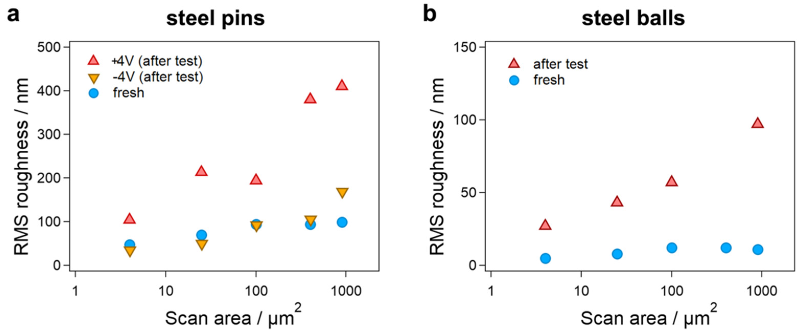
¹H-NMR spectra were measured with a Bruker Avance (Bruker, Billerica, MA, USA) at 250 MHz. Deuterated water (D2O) served as the solvent. The spectra were calibrated to the solvent. The evaluation was performed using the ACD/NMR Processor Academic Edition software V12 (Advanced Chemistry Development, Inc., Toronto, ON, Canada).

2.7. Wear Analysis

After testing, wear was determined using a 3D laser microscope VK-9710K (Keyence, Osaka, Japan). Both the wear volume and the wear area were determined. Due to the very low wear observed on the ball, only the wear on the pins was considered. Furthermore, the surface topography of these samples was measured via AFM-based imaging to estimate the surface roughness before and after tribological loading.

3. Results

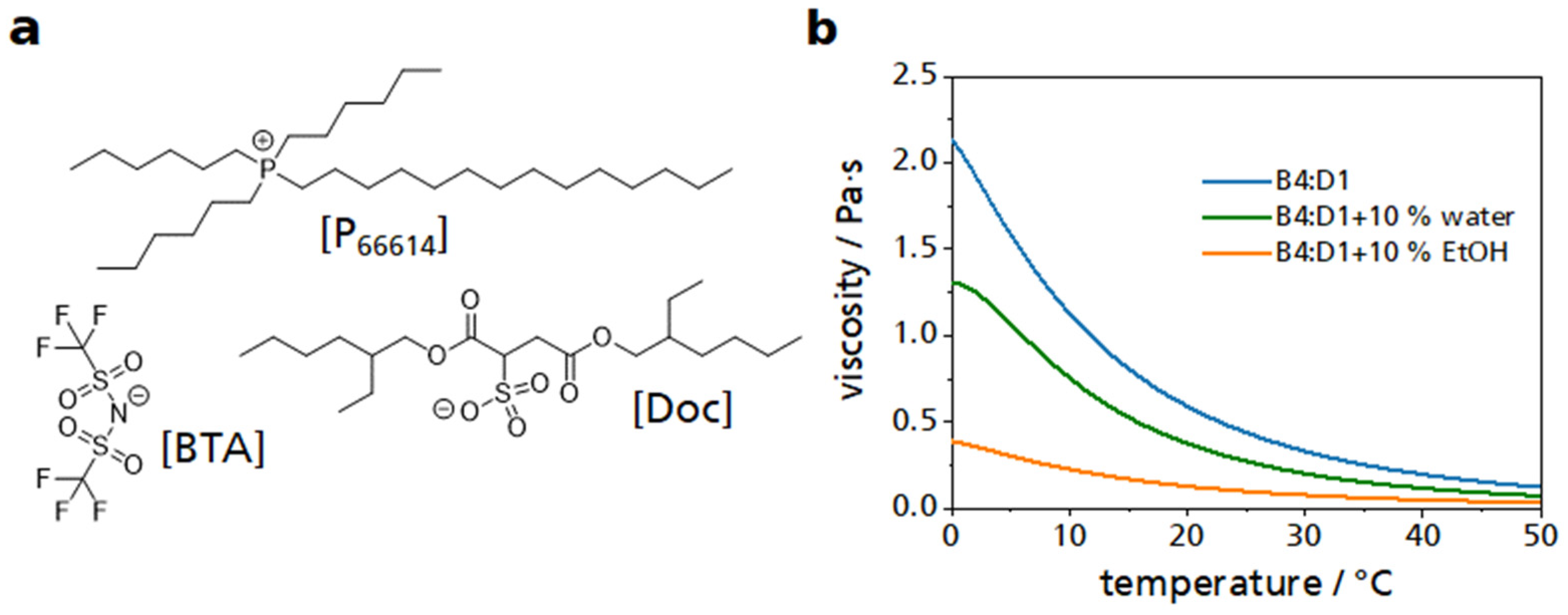
3.1. Viscosity and Pressure–Viscosity Coefficient

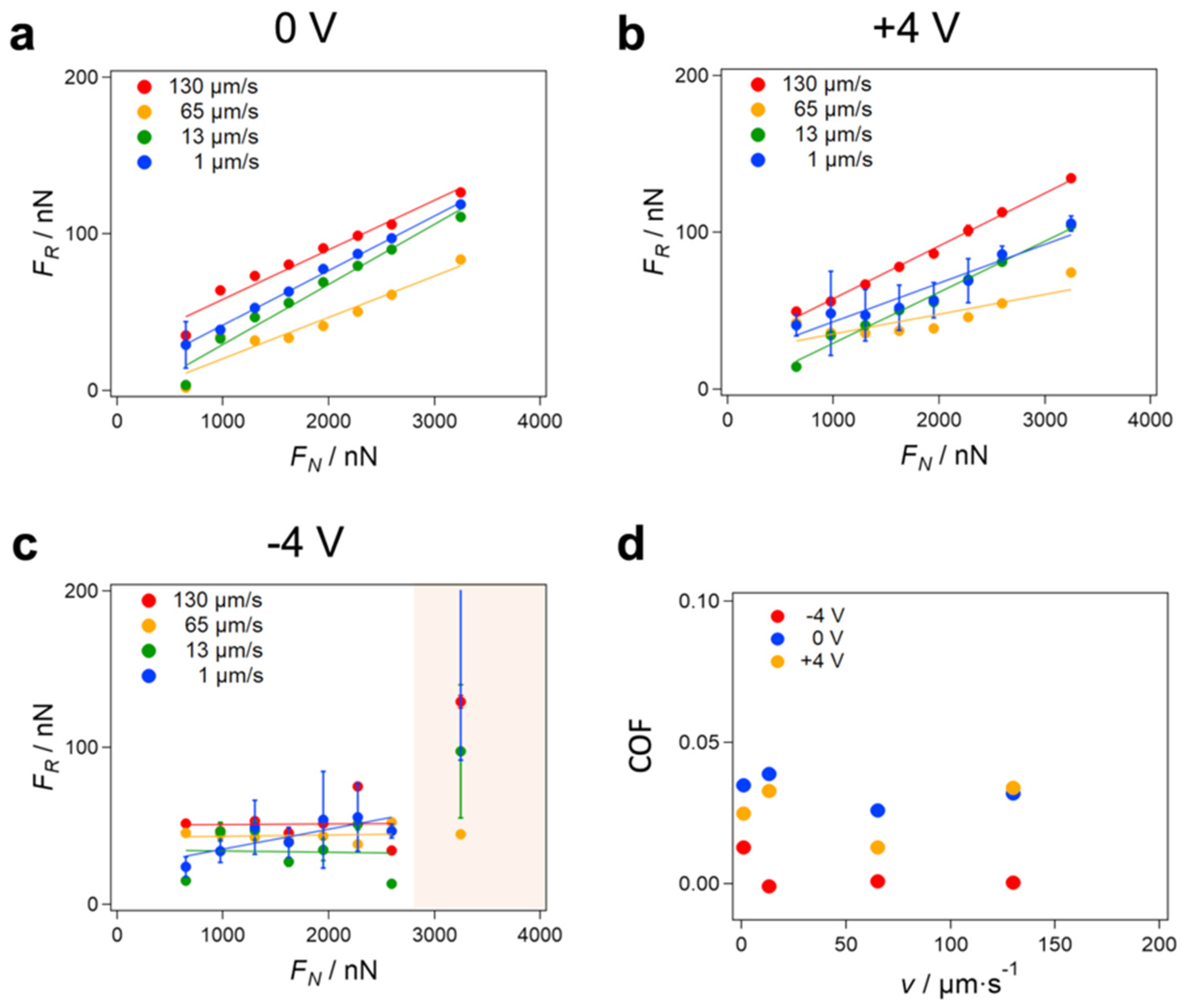
As a basis for the following tribological studies, the viscosity of the lubricants used was measured using the MCR501 rheometer. The lubricant was placed between two plates and sheared by rotating one of the plates. The shear rate (50 s⁻¹) remained constant, and the viscosity was measured as a function of temperature (Figure 1). Although the shear was kept constant, it should be noted that for a plate–plate geometry, the shear increases with the radius of the plate from the inside to the outside and is not constant over the entire plate. Two commercially acquired ILs containing the same phosphonium cation [P66614] were used. One of the concomitant anions was a sulfosuccinate [Doc], the other a sulfonyl imide derivative [BTA] (Figure 1a). The tests were made with the ILM having a mass ratio [BTA] to [Doc] of 4:1 (in the following, this ILM is abbreviated as B4:D1). The selection of these two ILs was based on preliminary work, which had shown promising results [16].

The addition of the low-viscosity solvents water or ethanol to the ILM reduced the resulting viscosity of the ILM. The addition of ethanol caused the viscosity to decrease more strongly compared to water. Visually, a slight turbidity could be detected in the mixture between the ILM and water. The mixture with ethanol, on the other hand, was clear and transparent like the ILM.

To be able to make a statement about the lubricant film thickness between the two friction partners and thus about the friction regime in the further course of this work, the pressure viscosity coefficient was determined for the ILM. For this purpose, measurements were carried out on the rheometer MCR501 at ambient pressure and at 200 bar at a shear rate of 50 s⁻¹ and a temperature of 20 °C. The calculations based on Equation (2) resulted in a pressure–viscosity coefficient for the ILM of (3.15 ± 1.82) × 10⁻⁹ Pa⁻¹. For comparison, water has a pressure viscosity coefficient of 0, because the viscosity does not change with changing pressure. For reference purposes, also, a polyalphaolefin (PAO) oil with a pressure viscosity coefficient of 12.6 × 10⁻⁹ Pa⁻¹ at a temperature of 50 °C and glycerol with a value of 5.9 × 10⁻⁹ Pa⁻¹ at 30 °C were recorded.

3.2. Nanotribology

Next, the tribological behavior of the steel in interaction with the ILM was studied by utilizing friction force microscopy (FFM) [58,59,60,61,62]. Here, we used an AFM cantilever provided with a colloidal tip, i.e., a glass bead (10 μm diameter), as the probe, and a steel pin as the surface. Furthermore, we applied different electrical potentials to the steel surface (three-electrode setup).

Before the FFM tests, we first measured the adhesive force between the glass bead and the steel surface. [63,64,65,66] There, the glass bead was pressed onto the surface of the steel pin (Figure S5b) with a certain normal force (649–3245 nN), and then the glass bead was retracted from the surface with a constant velocity of 1 μm/s for a sufficiently long distance (2 µm), which was recorded by the AFM as the vertical force–extension curve. We found that the adhesion force remains undetectably low, irrespective of the applied normal forces and electrical potentials. Therefore, we could use the Hertzian contact model, neglecting the surface roughness of the contacting bodies, to estimate a lower limit of the contact pressure P and an upper limit of the contact area A, which were 0.2–0.5 GPa and 10³–10⁴ nm² in this study, respectively (Figure S5b,c, see the section AFM-based contact mechanics in the supporting information for details). Such a pressure is far lower than the pressure required for the plastic deformation of steel and glass [67,68] and indicates that the contact was still in a purely elastic deformation regime.

Then, we carried out FFM experiments to determine the friction force between the glass bead and the steel surface (Figure 2a). Here, the experiments were carried out at different normal forces F_N (649–3245 nN) with varying scan velocities v (1–130 μm/s) and different electrical potentials applied to the steel surface. For each of the experiments, the glass bead was moved along the same single line for at least 64 times, where the scanning axis was perpendicular to the cantilever axis. As shown in Figure 2b,c, we obtained lateral force–distance curves for both trace and retrace, which are known as friction loops [51,52,53]. For these friction loops, we tried to use the same topographical line for the different measurement conditions applied. Thus, the obtained friction loops were not biased by topographical details (Figure S6) and could be directly compared to for different normal forces F_N and scan velocities v.

We carried out FFM experiments in an EC cell to build up an electric field throughout the ILM and measure the friction between the glass sphere and the steel pin with electrical potential differences of −4 V, 0 V, and +4 V. At this point, it is important to mention once that the IR-drop must be considered for all voltages given in this work. This represents the internal voltage drop due to the resistance of any conductor. In this case, ILs were used as conductors that can form a double layer at the electrode, which in turn results in an increase in the internal resistance and thus an increase in the IR-drop. As shown in Figure 3a, F_R increased linearly with the F_N for 0 V. Thus, we could determine the COF μ using Amontons’ law, F_R = μ F_N. Furthermore, the obtained friction force F_R and COF at 0 V and +4 V were very similar for the whole range data (Figure 3a,b). However, when a potential of −4 V (Figure 3c) and normal forces F_N in the 600 to 2500 nN range were applied, the COF was significantly smaller than those obtained for 0 V and +4 V. For larger normal forces F_N, the friction forces F_R increased strongly.

Next, we investigated the velocity dependence of the F_R by carrying out the FFM experiments with scan velocities from 1 to 130 μm/s. For each F_N, we varied the scan velocities from 1 to 130 μm/s on the same topographical line to avoid any impact of possible topographical change on the velocity dependence observed. For all applied electrical potentials (0 V and ±4 V), a slight velocity dependence of F_R was observed (see Figure 2 for exemplary friction loops). For 0 V and +4 V, the COF stayed rather constant in a wide velocity range, except around 65 µm/s, where the COF decreased. For −4 V for all normal forces F_N in the 600 to 2500 nN range, the COF stayed almost constant with increasing velocity and was significantly below the COFs for 0 V and +4 V for all scan velocities (Figure 3d). Such a low velocity dependence suggests that the F_R originates from boundary lubrication and that viscous friction, which would lead to a velocity dependency of the friction force, appears to be negligible. This conclusion is further corroborated by FFM experiments in bulk liquid when the bead was retracted far away from the surface. In that case, the measured friction resulted from the viscous friction of the ILM only. There, the measured friction force F_R was around 1 nN, which was more than an order of magnitude lower compared to the F_R at the contact between the glass bead and the steel surface, as shown in Figure S7.

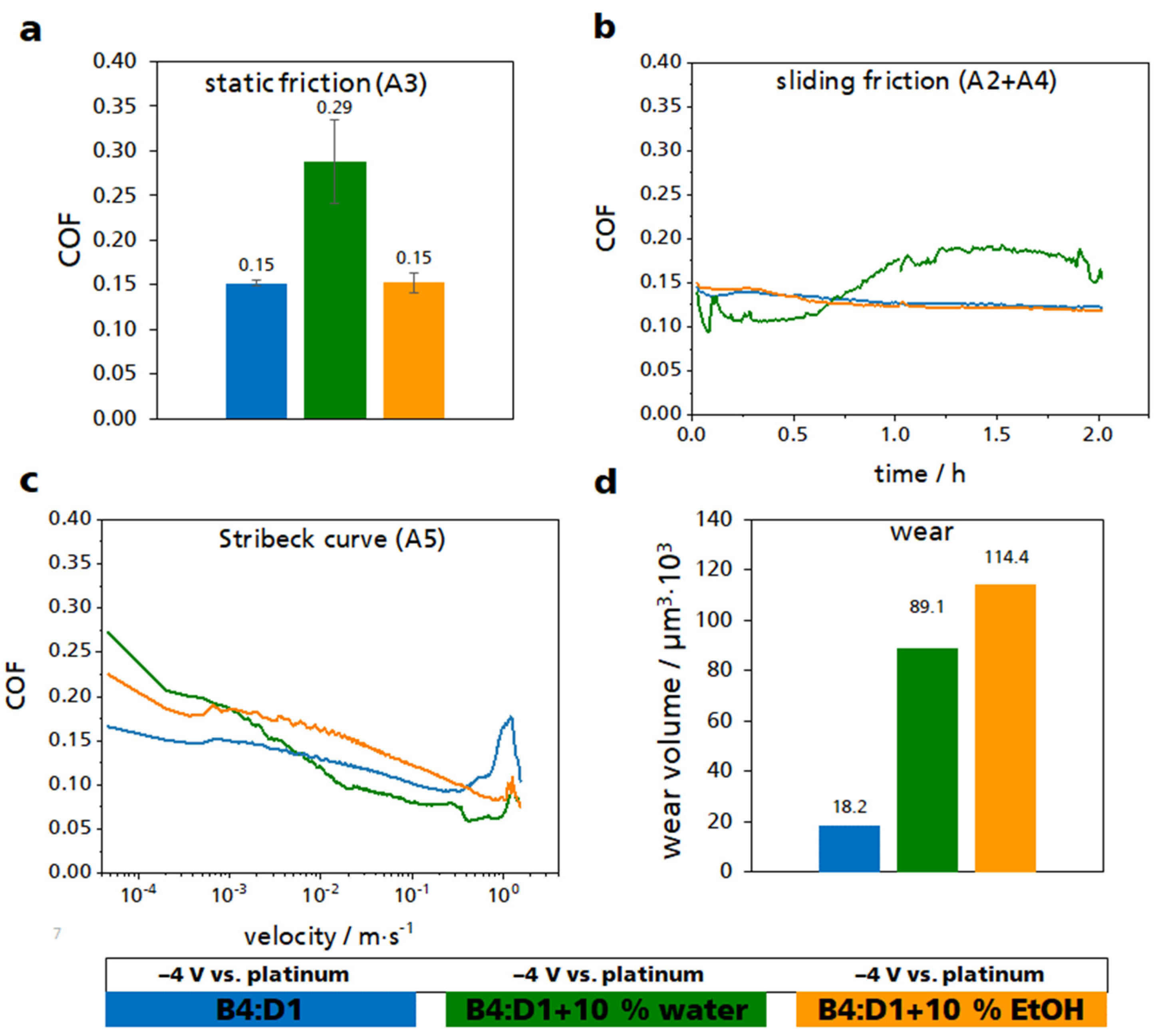
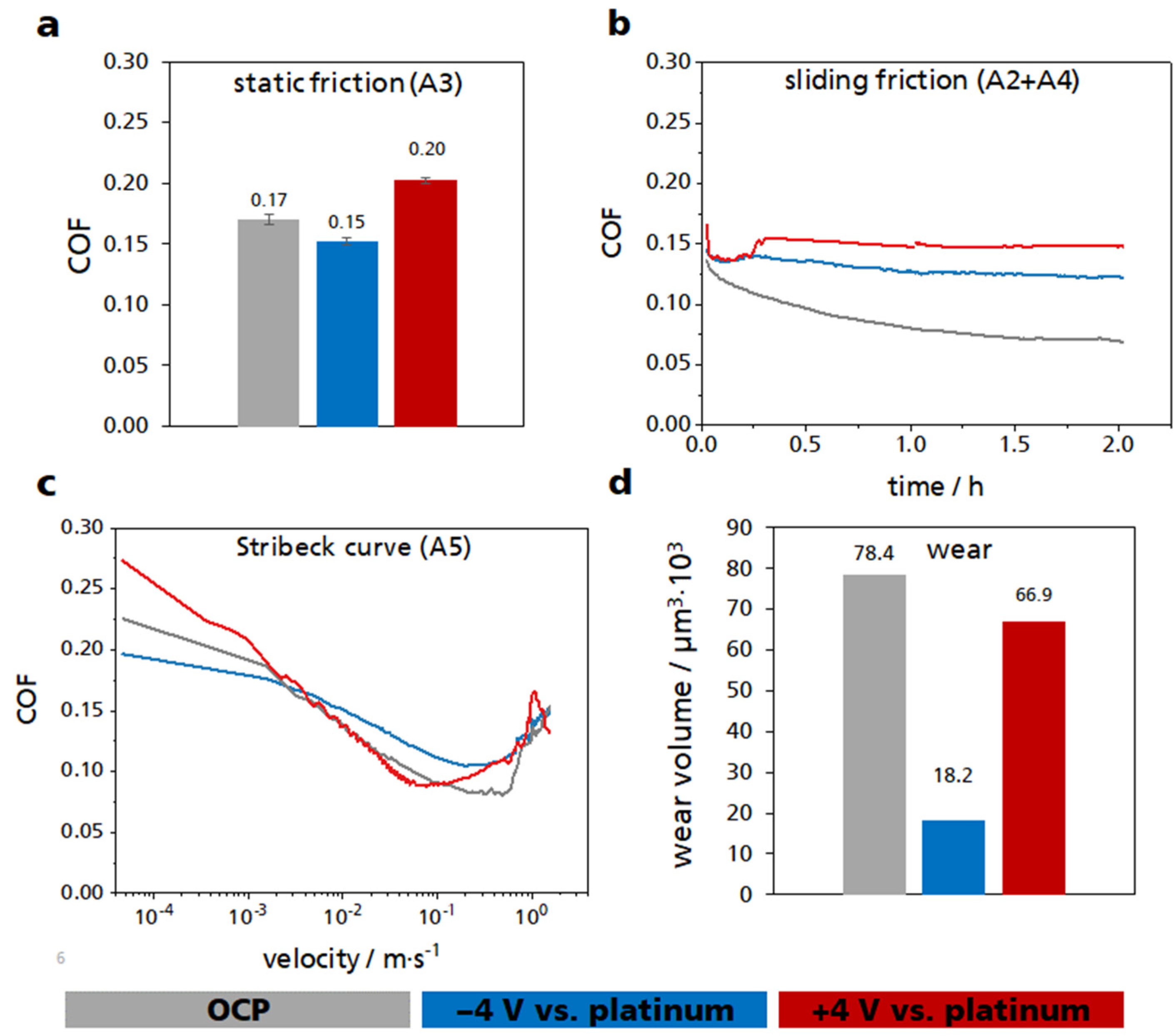
3.3. Macroscopic Tribology

The experimental setup for determining the macroscopic friction behavior consisted of a tribological cell connected to a potentiostat. The three lower pins were contacted as electrochemical working electrodes (WE). This allowed us to induce an electrochemical surface charge in the sliding contact, which was also transferred to the rotating ball [16]. The controllability of the COF in this two-electrode setup was tested with a constant potential (OCP, −4 V, +4 V) between the WE and the counter electrode (CE), resulting in either an anodically or cathodically charged surface. ILM B4:D1 was used as a lubricant. Tribological tests were performed with a normal force of 5 N (2.36 N per pin) on a ½ inch 100Cr6 steel ball. At room temperature, both static friction and dynamic friction properties were determined. Figure 4 shows the results from the experiment at different applied electrical potentials. In the case of static friction, only the second static friction test A3 is shown, because the first measurement A1 depended very strongly on the surface properties of the material and did not reflect the relation between electric potential and ILM. The result of the measurement of A1 is presented in Figure S8. In addition, the current curves of the anodic and cathodic tests are plotted in Figure S8.

Figure 4a shows the static friction value of the two friction partners ball and three pins with respect to the different applied electrical potentials. Without an applied potential, the mean value of the five measured values was COF = 0.17. With an applied potential, the static friction value could be changed significantly compared to the measured values of the open circuit electrical potential (OCP). With a cathodic potential of −4 V, the static COF can be reduced by approximately 12% to 0.15 compared to the value at the OCP (0.17). At an anodic potential of +4 V, static COF increased by approximately 18% to 0.20 compared to OCP.

The sliding friction could also be influenced by applying a potential (Figure 4b). Here, both the application of a cathodic and the anodic potential increased the COF. Towards the end of the test, the COF without applied potential reached a value of about 0.07. With continuous cathodic potential, a COF of 0.12 was reached at the end of the test, which corresponded to an increase of approximately 71% compared to the experiment without applied potential. Even with an anodic potential, the COF increased to 0.15 at the end, which was an increase of approximately 114% of the COF of the OCP test. The variability of the COF was also visible in the Stribeck curve (Figure 4c). Here, only the increasing velocity was used as the x-axis. The other two components of the Stribeck parameter, the viscosity of the lubricant and the normal force were kept constant. Especially at very low rotational velocity, a difference in COF between the different electrical potentials could be seen. At low velocity, the result reflected the static friction. With an anodic potential, an increase in COF compared to COF at OCP could be seen. A cathodic potential caused a decrease in the COF compared to the COF at OCP.

Not only could the COF be influenced with an external electrical potential, but also the wear (Figure 4d). The wear of the ball was neglected in this measurement because it was very small compared to the wear of the pins. It can be clearly seen that by applying a potential, whether anodic or cathodic, the wear could be reduced, i.e. by approximately 77% by applying a cathodic potential and by approximately 15% with an anodic potential compared to the result of the OCP test. The system used had a higher wear rate than typical applications running in this friction regime. However, the focus of this work was solely to investigate the influence of the potential change on the friction coefficient and how to control the latter. It is also important to consider that pure ionic fluids were used here, rather than a fully additivated oil. The 3D laser microscope images of the wear surfaces of the pins are shown in Figure S9. From the calculated wear area of the pins, the roughness, and the measured pressure–viscosity coefficient, the lubricant film thickness of these three tests was calculated at the end of the test using the Hamrock–Dowson equation (Equation (4)).

The calculated central lubricant film thickness for the test performed at OCP was 33 nm. At −4 V, the lubricant film thickness at the end of the test was 31 nm, and for the test at +4 V, it was 32 nm.

In addition, the measurements performed with the ILM B4:D1 were also performed with 10% water and 10% ethanol. The objective was to evaluate the influence of hydrogen bonding on the change in COF at electrical potentials. The results of these measurements are shown in Figure 5. The results of the ILM B4:D1 at cathodic potential are shown again in this graph for comparison.

Figure 5a shows the static friction of the three lubricants used. The mixture with 10% ethanol had the same static friction value of 0.15 as the ILM B4:D1. The mixture with water showed an increased COF of approximately 93% compared to the other two lubricants. A similar picture was also observed for the sliding friction (Figure 5b). Although the COF of the water mixture had initially been lower than that of the other two mixtures, at a duration of 45 min, there was an intersection of the graphs, after which the water mixture showed an increased COF. At the end of the test, the COF was approximately 27% higher than by using ILM B4:D1. The course of the ethanol mixture was hardly distinguishable from the ILM. At the end of the test, a reduction in COF of around 2% could be observed. In the Stribeck curve, a higher COF could be observed for both the water mixture and the ethanol mixture compared to the ILM for low rotational velocities (Figure 5c). By contrast, at high rotational velocities, the water mixture exhibited a lower COF than the ILM. The differences in wear were very pronounced (Figure 5d). Here, the addition of water or ethanol led to an increase in wear. With water, wear increased by approximately 390% compared to the ILM, and with ethanol by approximately 530%. The images of the wear surfaces are shown in Figure S9.

3.4. Wear Analysis

AFM imaging on steel pins and steel balls was conducted to evaluate the surface wear caused by tribometer experiments. Here, the samples of the multi-experiment were measured, the results of which are shown in Figure 4. Scans were taken at 30∙30, 20∙20, 10∙10, 5∙5, and 2∙2 μm, so that roughness could be estimated at different scales (Figures S10 and S11, as well as Tables S1 and S2 for details). Note that the AFM-based imaging delivers topographical information at the micrometer scale, i.e., a local information of the sample surface. Thus, the RMS roughness values might vary with the respective local spots on the samples, which may differ largely from the roughness at the macroscopic level. Such scale dependence of roughness is supported by a recent research on using the power spectral density to describe the roughness, which showed that roughness is a multiscale material parameter that can vary across many orders of length scales [69].

For all steel pins (before and after ±4 V tribometer tests), it was found that the RMS roughness increased with increasing scan size (Figure 6a). This is mainly associated with local topography, where more asperities were involved with expansion of the area, leading to a higher RMS roughness. Moreover, we observed a marked increase in RMS roughness after the +4 V tribometer test, while it remained low after the −4 V tribometer test, comparable to the fresh steel pin. These results were in good agreement with the measured COF at different electrical potentials and the corresponding wear (Figure 4). Similar results were found for steel balls (Figure 6b): the RMS roughness increased largely after the tribometer test, indicating severe wear at the surface. Altogether, these findings validate that the tribological behavior and wear of steel in the ILM were dependent on the external electrical potential.

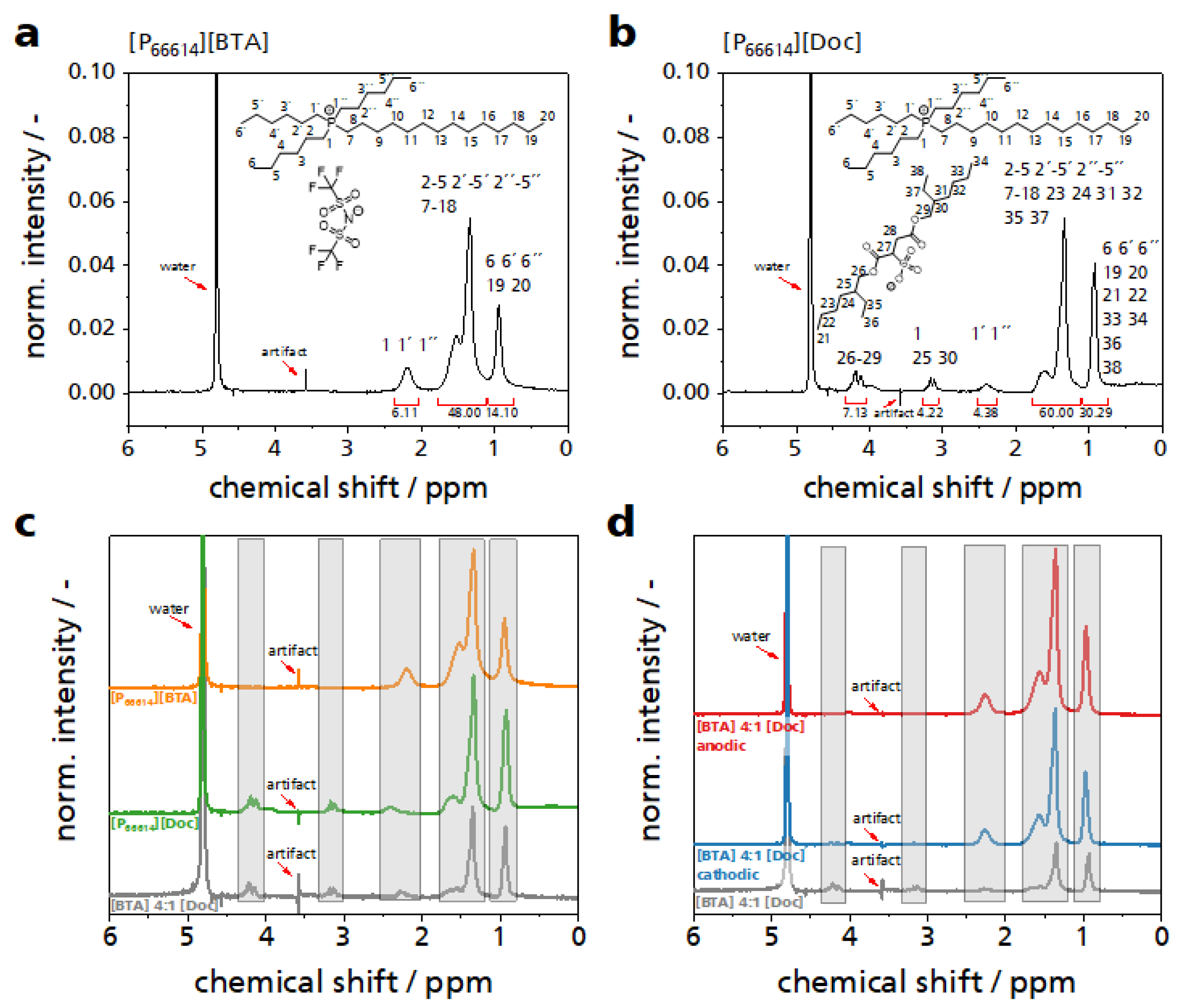
3.5. NMR Spectroscopy

In order to check whether chemical reactions already took place when the two ILs are mixed, and to see how the ILM reacted when exposed to a potential that leads to degradation, ¹H-NMR measurements were performed. In addition, solid-state NMR measurements were also performed, showing that even after applying high voltages for a long period of time no high molecular weight compounds are formed (Figure S12). Both the two ILs per se and the mixture were investigated. In addition, it was studied how the ILM decompose at anodic and cathodic potential when the system is operated outside the electrochemically stable window (Figure 7).

The spectrum of the [BTA] variant reflected the large number of aliphatic protons (0.9–1.6 ppm) present in the IL (Figure 7a). Only the six protons directly bonded to the phosphorus atom showed a low field shift (2.2 ppm). The anion does not contain any protons and accordingly does not contribute to the spectrum. In the spectrum of the [Doc] variant, some protons present in the anion show signals with a significant low field shift (3.1 and 4.1 ppm, Figure 7b). Comparing the two IL it is interesting to note that the signals of the protons in the same cation show a slightly different shift in the [Doc] variant compared to the [BTA] variant depending on the anion present (Figure 7c). In the [Doc] variant the protons directly bound to the phosphorus atom experienced a stronger low field shift (2.4 ppm) than in the [BTA] variant (2.2 ppm). In the NMR spectrum of the ILM in comparison to the two IL components, all signals remain unchanged(gray bars, Figure 7c). When the voltage was increased up to ±10 V in steps of one volt, with each potential step held for 5 minutes, a visual change in the ILM was observed and the ILM showed a slightly brown color in both cases. When a potential of ±10 V is applied which is clearly outside of the electrochemical stable window, the NMR spectra change strongly indicating strong degradation (Figure 7d).

4. Discussion

When an external electrical potential is applied to a tribological system lubricated with an ILM, a change in COF is observed at both nanoscale and macroscale levels. As the charged molecules undergo orientation, adsorption, and electromigration upon an applied electrical potential, we assume that the application of the varying electrical potentials leads to an increase in the concentration of either the anion or the cation in the friction gap [11]. Due to the long alkyl chains and thus oil-like structure of the cation, a concentration increase in these compounds in the friction gap could lower the COF. Therefore, the COF decreases when a negative potential is applied. The beneficial effect of such tribo layers consisting of cations was particularly evident in the wear of the pins tested at a potential of −4 V (Figure 4c). A reduction of the wear by about 77% is a very significant lowering. With a positive potential, the anions were increasingly driven into the friction gap. The smaller anions, which also have no long-chain structures, were not able to form such a lubricating film in the same way as the cations, and thus the COF increased. These observations were made both at the nano- and macroscales, although some differences between the macroscale tribometer and the nanoscale FFM experiments have to be considered as the FFM experiments covered a lower velocity range than the macroscopic experiments. Within this velocity range, the COFs obtained during the FFM experiments were mostly velocity independent (boundary lubrication regime of the Stribeck, see also Figure 4). Additionally, the FFM experiments averaged over a much smaller contact area (10³–10⁴ nm², Figure S5c) with fewer asperities than at the macroscale. Accordingly, the COF in FFM was one order of magnitude lower than in the macroscopic experiments. Furthermore, in the macroscopic experiments, a steel ball was measured against a steel surface, whereas for the FFM experiments, a glass bead was used on a steel surface.

It should be noted that the FFM experiments showed an increase in the COF at the largest normal force, even at −4 V. This could have been due to the high pressure causing a breakthrough through the ordered alkyl chains, which leads to increased boundary friction and thus high friction forces. It was also observed that at low velocities, the COF values showed strong experiment to experiment variations. These conditions could induce particularly small lubricant film thicknesses (Figure 4a,d). When the thickness is low, a small lubricant film thickness variation between the two friction bodies or a small variation of a change in the composition of the active tribo layers has a particularly large influence on friction. However, apart from these minor differences the trend of the two nano- and macroscale experiments was the same.

For an explanation why the IL mixtures respond more precisely and strongly to electrical potentials than the individual ILs alone, it could be hypothesized that the structure near the electrodes in a three-component system differs significantly from that of a two-component system. The different size of the ions could result in a different ion packing at the electrodes [70,71]. For the system used in this work, the two anions could form a more stable layer than without the respective other anion, which can also be clearly seen when comparing the results of the mixtures with the pure IL systems [16].

Furthermore, the calculated pressure viscosity coefficient was used to calculate the lubricant film thickness. Looking at the lubricant film thickness, the difference between OCP and both positive and negative voltage was not significant (OCP: 33.5 nm, −4 V: 31.4 nm, +4 V: 32.6 nm). However, when the lubricating film thickness and the size of the ions were calculated with the tool Avagadro (P66614: 27.13 Å, BTA: 7.27 Å, Doc: 18.86 Å), significant differences were observed. It is assumed that at OCP, all three ions and thus the mean value of all three ions must be considered, while with a positive charge, only the two anions are in the friction gap, and with a negative charge, only the cations are relevant. This results in significantly different layer numbers of the lubricating film for the individual experiments. At OCP, there were approximately 19 layers of anions and cations in the friction gap, with a negative potential approximately 12 layers of cations and with a positive potential approximately 25 layers of anions. This correlates nicely with the decrease in the COFs.

In addition, it was investigated to which extent hydrogen bonds introduced to the ILM by water or ethanol could alter the layer formation under the influence of an external electrical potential. It was found that the addition of ethanol at a voltage of −4 V changed both static and dynamic friction only slightly compared to the ILM. Only at very high velocities was an increase in COF observed, although the viscosity was significantly reduced by the addition of the ethanol (see Figure 1). With the addition of water, however, the COF showed a significant increase at a cathodic potential of −4 V in both static and sliding friction. At high velocities, a decrease in COF was obtained in the Stribeck curve. Water mitigates the interactions between the IL molecules and thus reduces the molecular orientation in the friction gap. This would explain the small differences in the COF between the pure and ethanol-doped ILM and the strong degradation of the behavior by adding a relatively small amount of water.

Furthermore, an improved stability of the ILM compared to the pure IL regarding the application of different electrical potentials is reported [72]. Wide potential windows in which the ILM was stable could be measured both at the nanoscale and at the macroscale range (Figure S4). To ensure multiple switching of the COF and stable tribological conditions, any ILM decomposition due to the electrical current flow has to be prevented. During the friction test, a small electrical current flows continuously [16]. It is assumed that this current is needed to carry ions repeatedly to the steel surface as they are tribologically sheared off, thus maintaining the tribologically active layer of ionic liquids. In Figure S8, the current as a function of time of an anodic and cathodic multi-experiment are plotted. The current flow was in the low µA range. Since it was difficult to determine a total resistance for the system in tribological contact and due to the IR drop, it was also not possible to determine exactly how much of the energy introduced by the electrical potential was dissipated into, e.g., heat. However, the NMR measurements showed that no chemical reactions occurred when the individual IL components were mixed or kept a low potentials, since the signals in the NMR spectrum of the ILM could be clearly assigned to the two pure ILs. By applying a voltage outside the stable window of the ILM, the NMR spectra showed that the anions tended to degrade, since the signals of the anions could no longer be detected in the NMR spectrum after both the anodic loading and the cathodic loading. It can be assumed that the functional groups of the anions are irreversibly oxidized or reduced by the increased potential. These results indicate that the low Faradayic current flowing during the friction experiments does not indicate lubricant degradation but are just caused by changes in the capacitive charging of the system.

5. Conclusions

The use of ILMs in both macroscopic and nanoscopic tribological systems can induce a change of COFs by electrical potentials. While the trends of the friction behavior of the ILM in nano- and macrotribology were similar, the values were numerically different because the contact area and the sliding velocity were different. In the nanotribology experiments, it was found that at a higher normal force, the tribo layers formed seemed to be much more stable in ILMs than in pure ILs. However, when the force was becoming too high, the layers presumably could break, and thus the lubrication effect was no longer present. Nevertheless, similar pressures and the same electrical potentials were used. Thus, it was possible to compare the macroscopic behavior with the nanoscale behavior of ionic liquids under electrochemical stress.

With the help of the calculated lubricant film thicknesses, it was possible to estimate the number of molecular layers within the friction gap and thus to draw a connection between COF and molecular density, which could explain the better tribological behavior of the mixtures in comparison to the pure components. In addition, it could be shown that the addition of ethanol and especially water to the IL, as well as the resulting changes in the hydrogen bonding of the systems, decreased the effect of the change in COF. NMR measurements revealed that no chemical reactions took place when the ILs were mixed and kept at low potentials, but that the anions in particular decomposed when the potential was too high, both at anodic and cathodic potentials.

In summary, the combination of theoretical considerations concerning the layer numbers, friction, NMR, rheology and FFM results provide an important insight in understanding the mechanisms of switchable and programmable friction with ILMs. The key factor seems to be molecular packing and orientation of the components of the mixtures.

In further work, investigations with altered chemical structure of the ILs and ILMs should be carried out to be able to draw more conclusions on the connection between structure and layer formation and the friction properties. In addition, further investigations are necessary to identify the relationship between electrical potential and electrochemical reactions at the surface of the friction partners.

References

1. Holmberg, K.; Erdemir, A. The impact of tribology on energy use and CO2 emission globally and in combustion engine and electric cars. Tribol. Int. 2019, 135, 389–396. [Google Scholar] [CrossRef]
2. Meng, Y.; Xu, J.; Ma, L.; Jin, Z.; Prakash, B.; Ma, T.; Wang, W. A review of advances in tribology in 2020–2021. Friction 2022, 10, 1443–1595. [Google Scholar] [CrossRef]
3. Luo, J.; Liu, M.; Ma, L. Origin of friction and the new frictionless technology—Superlubricity: Advancements and future outlook. Nano Energy 2021, 86, 106092. [Google Scholar] [CrossRef]
4. Cai, W.; Trefs, J.L.; Hugel, T.; Balzer, B.N. Anisotropy of π–π Stacking as Basis for Superlubricity. ACS Mater. Lett. 2023, 5, 172–179. [Google Scholar] [CrossRef]
5. Adibnia, V.; Mirbagheri, M.; Faivre, J.; Robert, J.; Lee, J.; Matyjaszewski, K.; Lee, D.W.; Banquy, X. Bioinspired polymers for lubrication and wear resistance. Prog. Polym. Sci. 2020, 110, 101298. [Google Scholar] [CrossRef]
6. Cecilia, J.A.; Ballesteros Plata, D.; Alves Saboya, R.M.; Tavares de Luna, F.M.; Cavalcante, C.L.; Rodríguez-Castellón, E. An Overview of the Biolubricant Production Process: Challenges and Future Perspectives. Processes 2020, 8, 257. [Google Scholar] [CrossRef]
7. Shah, R.; Woydt, M.; Zhang, S. The Economic and Environmental Significance of Sustainable Lubricants. Lubricants 2021, 9, 21. [Google Scholar] [CrossRef]
8. Amiril, S.; Rahim, E.A.; Syahrullail, S. A review on ionic liquids as sustainable lubricants in manufacturing and engineering: Recent research, performance, and applications. J. Clean. Prod. 2017, 168, 1571–1589. [Google Scholar] [CrossRef]
9. Naveed, T.; Zahid, R.; Mufti, R.A.; Waqas, M.; Hanif, M.T. A review on tribological performance of ionic liquids as additives to bio lubricants. Proc. Inst. Mech. Eng. Part. J. J. Eng. Tribol. 2021, 235, 1782–1806. [Google Scholar] [CrossRef]
10. Ma, L.; Zhang, C.; Liu, S. Progress in experimental study of aqueous lubrication. Chin. Sci. Bull. 2012, 57, 2062–2069. [Google Scholar] [CrossRef]
11. Bresme, F.; Kornyshev, A.A.; Perkin, S.; Urbakh, M. Electrotunable friction with ionic liquid lubricants. Nat. Mater. 2022, 21, 848–858. [Google Scholar] [CrossRef]
12. Sharma, B.K.; Biresaw, G. Environmentally Friendly and Biobased Lubricants; CRC Press: Boca Raton, FL, USA, 2016; ISBN 9781482232035. [Google Scholar]
13. Tysoe, W.T.; Spencer, N.D. Rapid testing of tribotronic materials. Tribol. Lubr. Technol. 2021, 77, 76–77. [Google Scholar]
14. He, S.; Meng, Y.; Tian, Y.; Zuo, Y. Response Characteristics of the Potential-Controlled Friction of ZrO2/Stainless Steel Tribopairs in Sodium Dodecyl Sulfate Aqueous Solutions. Tribol. Lett. 2010, 38, 169–178. [Google Scholar] [CrossRef]
15. Glavatskih, S.; Höglund, E. Tribotronics—Towards active tribology. Tribol. Int. 2008, 41, 934–939. [Google Scholar] [CrossRef]
16. Gatti, F.; Amann, T.; Kailer, A.; Baltes, N.; Rühe, J.; Gumbsch, P. Towards programmable friction: Control of lubrication with ionic liquid mixtures by automated electrical regulation. Sci. Rep. 2020, 10, 17634. [Google Scholar] [CrossRef] [PubMed]
17. Krim, J. Controlling Friction With External Electric or Magnetic Fields: 25 Examples. Front. Mech. Eng. 2019, 5, 22. [Google Scholar] [CrossRef]
18. Fajardo, O.Y.; Bresme, F.; Kornyshev, A.A.; Urbakh, M. Electrotunable Friction with Ionic Liquid Lubricants: How Important Is the Molecular Structure of the Ions? J. Phys. Chem. Lett. 2015, 6, 3998–4004. [Google Scholar] [CrossRef] [PubMed]
19. Liu, C.; Li, X.; Li, X.; Li, W.; Tian, Y.; Meng, Y. On-Line Feedback Control of Sliding Friction of Metals Lubricated by Adsorbed Boundary SDS Films. Lubricants 2022, 10, 148. [Google Scholar] [CrossRef]
20. David, A.; Fajardo, O.Y.; Kornyshev, A.A.; Urbakh, M.; Bresme, F. Electrotunable lubricity with ionic liquids: The influence of nanoscale roughness. Faraday Discuss. 2017, 199, 279–297. [Google Scholar] [CrossRef]
21. Comtet, J.; Niguès, A.; Kaiser, V.; Coasne, B.; Bocquet, L.; Siria, A. Nanoscale capillary freezing of ionic liquids confined between metallic interfaces and the role of electronic screening. Nat. Mater. 2017, 16, 634–639. [Google Scholar] [CrossRef]
22. Fedorov, M.V.; Kornyshev, A.A. Ionic liquids at electrified interfaces. Chem. Rev. 2014, 114, 2978–3036. [Google Scholar] [CrossRef] [PubMed]
23. Raviv, U.; Klein, J. Fluidity of bound hydration layers. Science 2002, 297, 1540–1543. [Google Scholar] [CrossRef] [PubMed]
24. Zhang, C.; Chen, J.; Liu, M.; Wang, F.; Zheng, Y.; Cheng, Y.; Liu, Z. Relationship between Viscosity and Resistance of Oil Film: A New Way to Investigate the Controllable Friction between Charged Interfaces Lubricated by Ionic Lubricating Oil. Adv. Mater. Interfaces 2022, 9, 2200229. [Google Scholar] [CrossRef]
25. Reddy, A.B.; Pilkington, G.A.; Rutland, M.W.; Glavatskih, S. Tribotronic control of an ionic boundary layer in operando extends the limits of lubrication. Sci. Rep. 2022, 12, 20479. [Google Scholar] [CrossRef]
26. Li, H.; Wood, R.J.; Rutland, M.W.; Atkin, R. An ionic liquid lubricant enables superlubricity to be “switched on” in situ using an electrical potential. Chem. Commun. 2014, 50, 4368–4370. [Google Scholar] [CrossRef] [PubMed]
27. Liu, C.; Fang, J.; Wen, X.; Tian, Y.; Meng, Y. Active Control of Boundary Lubrication of Ceramic Tribo-Pairs in Sodium Dodecyl Sulfate Aqueous Solutions. Tribol. Lett. 2021, 69, 144. [Google Scholar] [CrossRef]
28. Amann, T.; Waidele, M.; Kailer, A. Analysis of mechanical and chemical mechanisms on cavitation erosion-corrosion of steels in salt water using electrochemical methods. Tribol. Int. 2018, 124, 238–246. [Google Scholar] [CrossRef]
29. Gatti, S.F.; Gatti, F.; Amann, T.; Kailer, A.; Moser, K.; Weiss, P.; Seidel, C.; Rühe, J. Tribological performance of electrically conductive and self-lubricating polypropylene-ionic-liquid composites. RSC Adv. 2023, 13, 8000–8014. [Google Scholar] [CrossRef]
30. Amann, T.; Kailer, A.; Herrmann, M. Influence of Electrochemical Potentials on the Tribological Behavior of Silicon Carbide and Diamond-Coated Silicon Carbide. J. Bio Tribo Corros. 2015, 1, 30. [Google Scholar] [CrossRef]
31. Kailer, A.; Amann, T.; Krummhauer, O.; Herrmann, M.; Sydow, U.; Schneider, M. Influence of electric potentials on the tribological behaviour of silicon carbide. Wear 2011, 271, 1922–1927. [Google Scholar] [CrossRef]
32. Amann, T.; Gatti, F.; Oberle, N.; Kailer, A.; Rühe, J. Galvanically induced potentials to enable minimal tribochemical wear of stainless steel lubricated with sodium chloride and ionic liquid aqueous solution. Friction 2018, 6, 230–242. [Google Scholar] [CrossRef]
33. Amann, T.; Dold, C.; Kailer, A. Potential Controlled Tribological Behavior of Water-Based Ionic Liquids. KEM 2016, 674, 250–256. [Google Scholar] [CrossRef]
34. Dold, C.; Amann, T.; Kailer, A. Influence of electric potentials on friction of sliding contacts lubricated by an ionic liquid. Phys. Chem. Chem. Phys. 2015, 17, 10339–10342. [Google Scholar] [CrossRef]
35. Gatti, F.; Amann, T.; Kailer, A.; Abicht, J.; Rabenecker, P.; Baltes, N.; Rühe, J. Makroskopische Reibwertsteuerung durch elektrochemische Potentiale mit ionischen Flüssigkeiten. Tribol. Und Schmier. 2019, 66, 51–57. [Google Scholar] [CrossRef]
36. Capozza, R.; Benassi, A.; Vanossi, A.; Tosatti, E. Electrical charging effects on the sliding friction of a model nano-confined ionic liquid. J. Chem. Phys. 2015, 143, 144703. [Google Scholar] [CrossRef]
37. Wang, Y.-L.; Golets, M.; Li, B.; Sarman, S.; Laaksonen, A. Interfacial Structures of Trihexyltetradecylphosphonium-bis(mandelato)borate Ionic Liquid Confined between Gold Electrodes. ACS Appl. Mater. Interfaces 2017, 9, 4976–4987. [Google Scholar] [CrossRef] [PubMed]
38. Shah, F.U.; Holmgren, A.; Rutland, M.W.; Glavatskih, S.; Antzutkin, O.N. Interfacial Behavior of Orthoborate Ionic Liquids at Inorganic Oxide Surfaces Probed by NMR, IR, and Raman Spectroscopy. J. Phys. Chem. C 2018, 122, 19687–19698. [Google Scholar] [CrossRef]
39. Pilkington, G.A.; Harris, K.; Bergendal, E.; Reddy, A.B.; Palsson, G.K.; Vorobiev, A.; Antzutkin, O.N.; Glavatskih, S.; Rutland, M.W. Electro-responsivity of ionic liquid boundary layers in a polar solvent revealed by neutron reflectance. J. Chem. Phys. 2018, 148, 193806. [Google Scholar] [CrossRef] [PubMed]
40. Ghazipour, H.; Gutiérrez, A.; Alavianmehr, M.M.; Hosseini, S.M.; Aparicio, S. Tuning the properties of ionic liquids by mixing with organic solvents: The case of 1-butyl-3-methylimidazolium glutamate with alkanols. J. Mol. Liq. 2021, 347, 117953. [Google Scholar] [CrossRef]
41. Lang, H.; Zou, K.; Chen, R.; Huang, Y.; Peng, Y. Role of Interfacial Water in the Tribological Behavior of Graphene in an Electric Field. Nano Lett. 2022, 22, 6055–6061. [Google Scholar] [CrossRef]
42. Espinosa-Marzal, R.M.; Arcifa, A.; Rossi, A.; Spencer, N.D. Microslips to "Avalanches" in Confined, Molecular Layers of Ionic Liquids. J. Phys. Chem. Lett. 2014, 5, 179–184. [Google Scholar] [CrossRef] [PubMed]
43. Espinosa-Marzal, R.M.; Arcifa, A.; Rossi, A.; Spencer, N.D. Ionic Liquids Confined in Hydrophilic Nanocontacts: Structure and Lubricity in the Presence of Water. J. Phys. Chem. C 2014, 118, 6491–6503. [Google Scholar] [CrossRef]
44. Smith, A.M.; Parkes, M.A.; Perkin, S. Molecular Friction Mechanisms Across Nanofilms of a Bilayer-Forming Ionic Liquid. J. Phys. Chem. Lett. 2014, 5, 4032–4037. [Google Scholar] [CrossRef]
45. Kawada, S.; Ogawa, S.; Sasaki, S.; Miyatake, M. Friction Control by Applying Electric Potential under Lubrication with Ionic Liquids. Tribol. Online 2019, 14, 71–77. [Google Scholar] [CrossRef]
46. Guo, Y.; Liu, G.; Li, G.; Zhao, F.; Zhang, L.; Guo, F.; Zhang, G. Solvent-free ionic silica nanofluids: Smart lubrication materials exhibiting remarkable responsiveness to weak electrical stimuli. Chem. Eng. J. 2020, 383, 123202. [Google Scholar] [CrossRef]
47. Michalec, M.; Svoboda, P.; Krupka, I.; Hartl, M.; Vencl, A. Investigation of the tribological performance of ionic liquids in non-conformal EHL contacts under electric field activation. Friction 2020, 8, 982–994. [Google Scholar] [CrossRef]
48. Yang, X.; Meng, Y.; Tian, Y. Effect of Imidazolium Ionic Liquid Additives on Lubrication Performance of Propylene Carbonate under Different Electrical Potentials. Tribol. Lett. 2014, 56, 161–169. [Google Scholar] [CrossRef]
49. Sader, J.E.; Chon, J.W.M.; Mulvaney, P. Calibration of rectangular atomic force microscope cantilevers. Rev. Sci. Instrum. 1999, 70, 3967–3969. [Google Scholar] [CrossRef]
50. Li, Q.; Kim, K.-S.; Rydberg, A. Lateral force calibration of an atomic force microscope with a diamagnetic levitation spring system. Rev. Sci. Instrum. 2006, 77, 65105. [Google Scholar] [CrossRef]
51. Filleter, T.; McChesney, J.L.; Bostwick, A.; Rotenberg, E.; Emtsev, K.V.; Seyller, T.; Horn, K.; Bennewitz, R. Friction and dissipation in epitaxial graphene films. Phys. Rev. Lett. 2009, 102, 86102. [Google Scholar] [CrossRef] [PubMed]
52. Gosvami, N.N.; Ma, J.; Carpick, R.W. An In Situ Method for Simultaneous Friction Measurements and Imaging of Interfacial Tribochemical Film Growth in Lubricated Contacts. Tribol. Lett. 2018, 66, 154. [Google Scholar] [CrossRef]
53. Ramakrishna, S.N.; Nalam, P.C.; Clasohm, L.Y.; Spencer, N.D. Study of adhesion and friction properties on a nanoparticle gradient surface: Transition from JKR to DMT contact mechanics. Langmuir 2013, 29, 175–182. [Google Scholar] [CrossRef] [PubMed]
54. Nečas, D.; Klapetek, P. Gwyddion: An open-source software for SPM data analysis. Open Phys. 2012, 10, 181–188. [Google Scholar] [CrossRef]
55. Gold, P.W.; Schmidt, A.; Dicke, H.; Loos, J.; Assmann, C. Viscosity–pressure–temperature behaviour of mineral and synthetic oils. J. Synth. Lubr. 2001, 18, 51–79. [Google Scholar] [CrossRef]
56. Hamrock, B.J.; Dowson, D. Isothermal Elastohydrodynamic Lubrication of Point Contacts: Part III—Fully Flooded Results. J. Lubr. Tech. 1977, 99, 264–275. [Google Scholar] [CrossRef]
57. Czichos, H.; Habig, K.-H. Tribologie-Handbuch: Tribometrie, Tribomaterialien, Tribotechnik, 4th ed.; Springer Vieweg: Wiesbaden, Germany, 2015. [Google Scholar]
58. Bennewitz, R.; Gnecco, E.; Gyalog, T.; Meyer, E. Atomic friction studies on well-defined surfaces. Tribol. Lett. 2001, 10, 51–56. [Google Scholar] [CrossRef]
59. Marchetto, D.; Held, C.; Hausen, F.; Wählisch, F.; Dienwiebel, M.; Bennewitz, R. Friction and Wear on Single-Layer Epitaxial Graphene in Multi-Asperity Contacts. Tribol. Lett. 2012, 48, 77–82. [Google Scholar] [CrossRef]
60. Kwon, S.; Lee, K.E.; Lee, H.; Koh, S.J.; Ko, J.-H.; Kim, Y.-H.; Kim, S.O.; Park, J.Y. The Effect of Thickness and Chemical Reduction of Graphene Oxide on Nanoscale Friction. J. Phys. Chem. B 2018, 122, 543–547. [Google Scholar] [CrossRef]
61. Chen, L.; Xiao, C.; He, X.; Yu, B.; Kim, S.H.; Qian, L. Friction and Tribochemical Wear Behaviors of Native Oxide Layer on Silicon at Nanoscale. Tribol. Lett. 2017, 65, 139. [Google Scholar] [CrossRef]
62. Wang, K.; Zhang, J.; Ma, T.; Liu, Y.; Song, A.; Chen, X.; Hu, Y.; Carpick, R.W.; Luo, J. Unraveling the Friction Evolution Mechanism of Diamond-Like Carbon Film during Nanoscale Running-In Process toward Superlubricity. Small 2021, 17, e2005607. [Google Scholar] [CrossRef]
63. Guo, D.; Li, J.; Xie, G.; Wang, Y.; Luo, J. Elastic properties of polystyrene nanospheres evaluated with atomic force microscopy: Size effect and error analysis. Langmuir 2014, 30, 7206–7212. [Google Scholar] [CrossRef] [PubMed]
64. Montagne, A.; Tromas, C.; Audurier, V.; Woirgard, J. A new insight on reversible deformation and incipient plasticity during nanoindentation test in MgO. J. Mater. Res. 2009, 24, 883–889. [Google Scholar] [CrossRef]
65. Mente, P.L.; Lewis, J.L. Elastic modulus of calcified cartilage is an order of magnitude less than that of subchondral bone. J. Orthop. Res. 1994, 12, 637–647. [Google Scholar] [CrossRef]
66. Bertoldi, K.; Reis, P.M.; Willshaw, S.; Mullin, T. Negative Poisson’s ratio behavior induced by an elastic instability. Adv. Mater. 2010, 22, 361–366. [Google Scholar] [CrossRef] [PubMed]
67. Young, M.L.; Almer, J.D.; Daymond, M.R.; Haeffner, D.R.; Dunand, D.C. Load partitioning between ferrite and cementite during elasto-plastic deformation of an ultrahigh-carbon steel. Acta Mater. 2007, 55, 1999–2011. [Google Scholar] [CrossRef]
68. Deschamps, T.; Martinet, C.; Neuville, D.R.; de Ligny, D.; Coussa-Simon, C.; Champagnon, B. Silica under hydrostatic pressure: A non continuous medium behavior. J. Non-Cryst. Solids 2009, 355, 2422–2424. [Google Scholar] [CrossRef]
69. Jacobs, T.D.B.; Pastewka, L.; Guest Editors. Surface topography as a material parameter. MRS Bull. 2022, 47, 1205–1210. [Google Scholar] [CrossRef]
70. Lian, C.; Liu, K.; van Aken, K.L.; Gogotsi, Y.; Wesolowski, D.J.; Liu, H.L.; Jiang, D.E.; Wu, J.Z. Enhancing the Capacitive Performance of Electric Double-Layer Capacitors with Ionic Liquid Mixtures. ACS Energy Lett. 2016, 1, 21–26. [Google Scholar] [CrossRef]
71. Osti, N.C.; Gallegos, A.; Dyatkin, B.; Wu, J.; Gogotsi, Y.; Mamontov, E. Mixed Ionic Liquid Improves Electrolyte Dynamics in Supercapacitors. J. Phys. Chem. C 2018, 122, 10476–10481. [Google Scholar] [CrossRef]
72. Siimenson, C.; Siinor, L.; Lust, K.; Lust, E. Electrochemical Characterization of Iodide Ions Adsorption Kinetics at Bi(111) Electrode from Three-Component Ionic Liquids Mixtures. ECS Electrochem. Lett. 2015, 4, H62–H65. [Google Scholar] [CrossRef]
Figure 1. Viscosity of ILMs. (a) Chemical structures of the ILs with the cation [P66614] and the two anions [BTA] and [Doc]. (b) Temperature-dependent viscosity of three ILMs. Shown in blue is the ILM of the two ILs. In green is the ILM plus 10% water, and in orange is the ILM with 10% ethanol.
Lubricants 11 00376 g001
Figure 2. FFM experiments between a glass bead and a steel surface in ILM. (a) Scheme of the experiment and of the lateral deflection of the cantilever for trace and retrace. Exemplary friction loops (lateral force-distance curves for trace and retrace) obtained at FN = 649 nN are shown for (b) a velocity v = 1 μm/s and (c) v = 130 μm/s. From left to right: electrical potentials applied to the steel surface −4, 0, and +4 V. The fluctuations of the lateral force profiles were also attributed to the topography change of the surface, as shown in Figure S6. However, the friction loop was not affected by those fluctuations.
Lubricants 11 00376 g002
Figure 3. Friction force under different conditions with an electric field throughout the ionic liquid in the EC cell. (ac) Friction force FR vs. normal force FN for the glass bead and the steel surface in the ionic liquid at different scan velocities v and electrical potentials differences (0, +4, −4 V). The COFs were obtained under the assumption of a linear dependence of FR on FN based on Amontons’ law. However, a clear deviation from a purely linear behavior was observed for −4 V, where the FR stayed rather constant, except for a strong increase at FN = 3245 nN (shaded area). (d) The COF obtained from the slope of the linear fits shown in (ac).
Lubricants 11 00376 g003
Figure 4. Multi-experiment with the sections A1–A5 with the ILM B4:D1. (a) Static friction values of the section A3. (b) Course of the friction value within the sliding friction experiments A2 and A4 (the curves of A2 and A4 were directly attached to each other, A2 from 0 to 1 h and A4 from 1 to 2 h). (c) Average course of the five recorded Stribeck curves in the section A5. (d) Wear volume of the three pins that served as a working electrode. The results measured at OCP are shown in gray, those of the anodic positive potential (+4 V) in red, and those of the cathodic negative potential (−4 V) in blue.
Lubricants 11 00376 g004
Figure 5. Multi-experiment with the sections A1–A5 using the ILM B4:D1 with either an addition of 10% water or 10% ethanol. (a) Static friction values of the section A3. (b) Course of the friction value within the sliding friction experiments A2 and A4. (c) Average course of the five recorded Stribeck curves in the section A5. (d) Sum wear of the three pins that served as a working electrode. All measurements were taken at a cathodic voltage of −4 V against a platinum wire. The results of ILM B4:D1 are shown in blue, those of the mixture with water in green, and those of the mixture with ethanol in orange.
Lubricants 11 00376 g005
Figure 6. Wear analysis of friction bodies. RMS roughness of (a) steel pins and (b) steel balls before and after tribometer experiments with ILM for AFM images with different scan sizes, indicated by scan areas.
Lubricants 11 00376 g006
Figure 7. 1H-NMR analysis of the studied ILs and ILMs. (a) NMR spectrum of the IL component [P66614][BTA]. (b) NMR spectrum of the IL component [P66614][Doc]. (c) NMR spectrum of the mixture [BTA] 4:1 [Doc] (gray line) with the spectra of the pure IL components ([BTA] orange line, [Doc] green line). (d) NMR spectrum of the mixture [BTA] 4:1 [Doc] (gray line) with the spectra of anodic (red line) and cathodic (blue line) loading out of the stable range. All NMR measurements were performed in deuterated water (D2O).
Lubricants 11 00376 g007
Disclaimer/Publisher’s Note: The statements, opinions and data contained in all publications are solely those of the individual author(s) and contributor(s) and not of MDPI and/or the editor(s). MDPI and/or the editor(s) disclaim responsibility for any injury to people or property resulting from any ideas, methods, instructions or products referred to in the content.