Machine Learning for Film Thickness Prediction in Elastohydrodynamic Lubricated Elliptical Contacts


Abstract
:1. Introduction
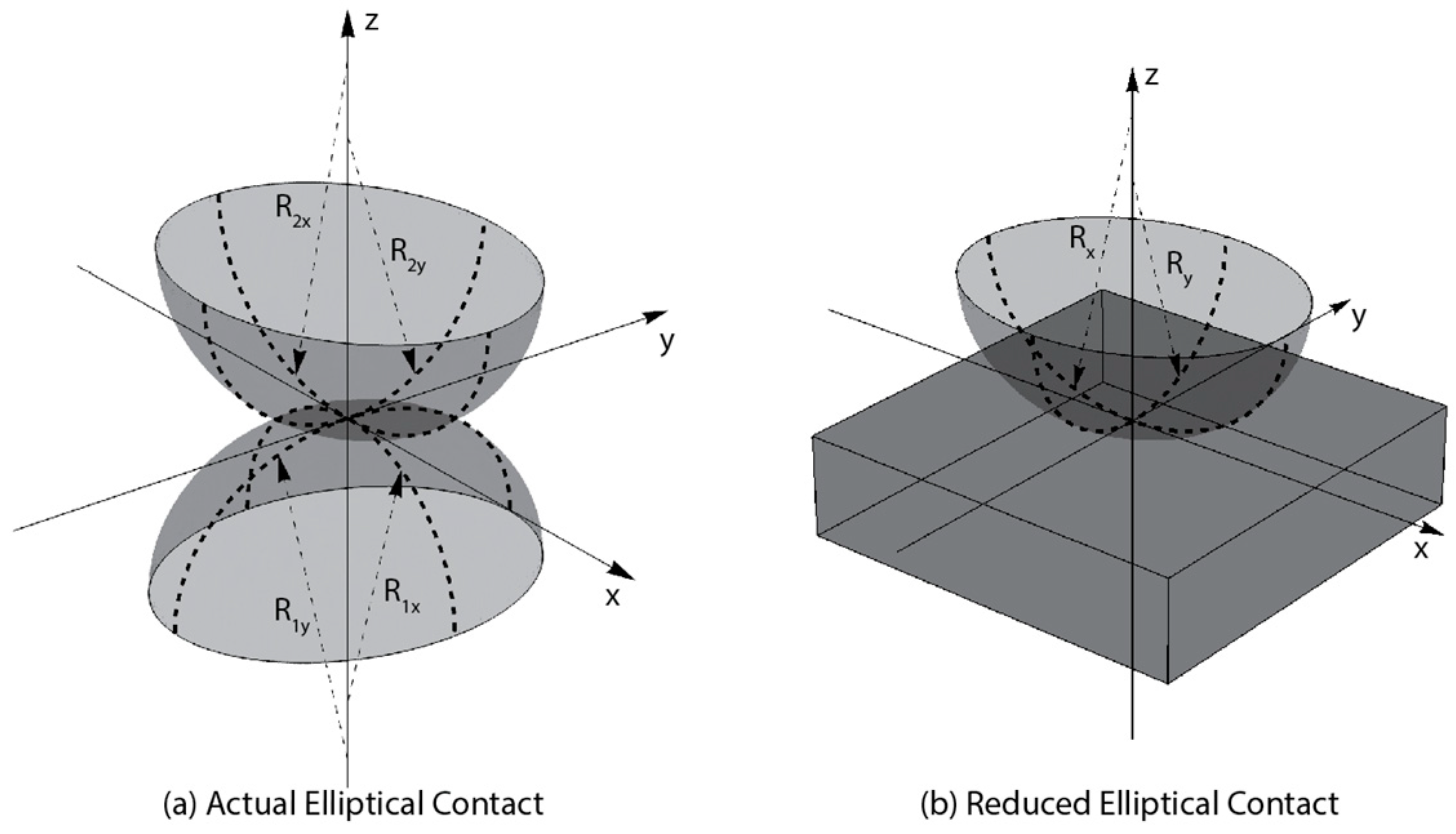
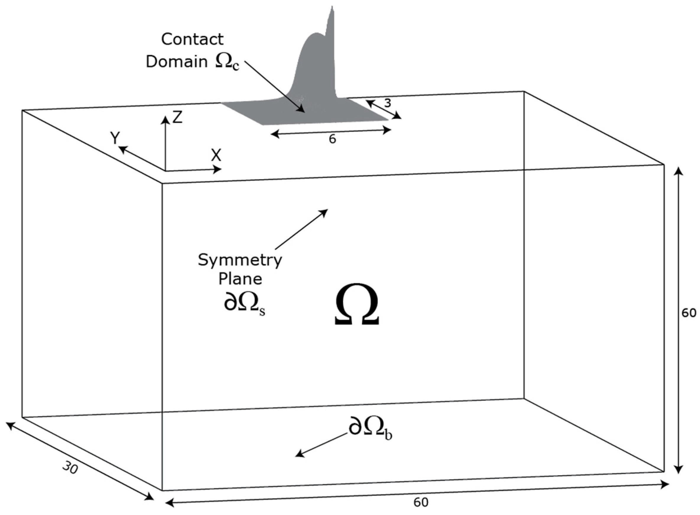
2. Finite Element Model
2.1. Governing Equations
2.2. Overall Numerical Procedure
2.3. Experimental Validation
3. Machine Learning
3.1. Data Generation
3.2. Feature Selection
3.3. Gaussian Process Regression (GPR)
4. Results and Discussion
5. Conclusions
Author Contributions
Funding
Data Availability Statement
Conflicts of Interest
Nomenclature
| Reciprocal asymptotic isoviscous pressure coefficient (Pa−1) | |
| Murnaghan EoS isothermal bulk modulus temperature coefficient (K−1) | |
| Lubricant low-shear/Newtonian viscosity (Pa·s) | |
| Dimensionless lubricant low-shear/Newtonian viscosity | |
| Lubricant viscosity at glass transition temperature (Pa·s) | |
| Lubricant low-shear/Newtonian viscosity at ambient pressure (Pa·s) | |
| , | Mean and standard deviation of features within the training dataset |
| Equivalent solid Poisson coefficient | |
| , | Poisson coefficient of solids 1 and 2 |
| Equivalent solid computational domain | |
| Contact computational domain | |
| Boundaries of | |
| Fixed boundary of | |
| Symmetry boundary of | |
| Complete elliptic integral of the first kind | |
| Lubricant density (kg/m3) | |
| Lubricant dimensionless density | |
| Lubricant density at ambient pressure (kg/m3) | |
| Normal component of 3D stress tensor (Pa) | |
| , , , | GPR model hyperparameters |
| Vector of tangential components of 3D stress tensor (Pa) | |
| Contact ellipticity ratio | |
| Shear stress in the j-direction within a plane having i as normal (Pa) | |
| , | Hertzian elliptical contact semi-axes in the x, y-directions (m) |
| , | Modified Yasutomi-WLF viscosity model parameters (°C) |
| , | Modified Yasutomi-WLF viscosity model parameters (Pa−1) |
| , | Modified Yasutomi-WLF viscosity model parameters |
| Ratio of contact equivalent radii of curvature and | |
| Equivalent solid Young’s modulus of elasticity (Pa) | |
| , | Young’s moduli of elasticity of solids 1 and 2 (Pa) |
| Contact external applied load (N) | |
| , , | Hamrock and Dowson material, speed, and load dimensionless groups |
| Lubricant film thickness (m) | |
| Central film thickness (m) | |
| Minimum film thickness (m) | |
| , | Dimensionless central film thickness |
| , | Dimensionless minimum film thickness |
| Dimensionless rigid-body separation | |
| , | Dimensionless lubricant film thickness |
| Isothermal bulk modulus at zero absolute temperature (Pa) | |
| Pressure rate of change of isothermal bulk modulus at zero pressure | |
| , | Moes dimensionless material properties and load parameters |
| , | Mean and kernel functions |
| , | Sizes of sample datasets , |
| Number of input features | |
| , | Number of samples in the training and testing datasets |
| Pressure (Pa) | |
| Hertzian contact pressure (Pa) | |
| Dimensionless pressure | |
| , | Principal radii of curvature of solids 1 and 2 in the xz-plane (m) |
| , | Principal radii of curvature of solids 1 and 2 in the yz-plane (m) |
| Radius of curvature of equivalent elastic solid in the xz-plane (m) | |
| Radius of curvature of equivalent elastic solid in the yz-plane (m) | |
| Equivalent radius of curvature of reduced contact geometry (m) | |
| Glass transition temperature (K) | |
| Glass transition temperature at zero pressure (K) | |
| Ambient temperature (K) | |
| , , | Equivalent solid deformation components in the x, y, z-directions (m) |
| , | Surface velocities of solids 1 and 2 in the x-direction (m/s) |
| Contact mean entrainment speed in the x-direction (m/s) | |
| , , | Solid dimensionless deformation components in x, y, z-directions |
| , , | Space coordinates (m) |
| , , | Gaussian distribution for standard, training and testing subsets |
| Prediction function of GPR model for testing samples | |
| , | Sample input features |
| , | Input i of , |
| Input feature number i | |
| Normalized value of input feature number i | |
| , , | Output variable i, its predicted and mean values in the testing dataset |
| , , | Dimensionless space coordinates |
| , | Training and testing sample datasets |
| , | Sample datasets |
Appendix A. Kernel Function Definitions
Appendix B. Data Standardization and Performance Metrics
References
- Holmberg, K.; Erdemir, A. Influence of Tribology on Global Energy Consumption, Costs and Emissions. Friction 2017, 5, 263–284. [Google Scholar] [CrossRef]
- Venner, C.H.; Lubrecht, A.A. Multi-Level Methods in Lubrication; Elsevier: Amsterdam, The Netherlands, 2000; ISBN 0-08-053709-X. [Google Scholar]
- Oh, K.P.; Rohde, S.M. Numerical Solution of the Point Contact Problem Using the Finite Element Method. Int. J. Numer. Methods Eng. 1977, 11, 1507–1518. [Google Scholar] [CrossRef]
- Ahmed, S.; Goodyer, C.E.; Jimack, P.K. An Adaptive Finite Element Procedure for Fully-Coupled Point Contact Elastohydrodynamic Lubrication Problems. Comput. Methods Appl. Mech. Eng. 2014, 282, 1–21. [Google Scholar] [CrossRef]
- Habchi, W. Finite Element Modeling of Elastohydrodynamic Lubrication Problems; John Wiley & Sons: Hoboken, NJ, USA, 2018; ISBN 1-119-22512-4. [Google Scholar]
- Lohner, T.; Ziegltrum, A.; Stemplinger, J.-P.; Stahl, K. Engineering Software Solution for Thermal Elastohydrodynamic Lubrication Using Multiphysics Software. Adv. Tribol. 2016, 2016, e6507203. [Google Scholar] [CrossRef]
- Tan, X.; Goodyer, C.E.; Jimack, P.K.; Taylor, R.I.; Walkley, M.A. Computational Approaches for Modelling Elastohydrodynamic Lubrication Using Multiphysics Software. Proc. Inst. Mech. Eng. Part J J. Eng. Tribol. 2012, 226, 463–480. [Google Scholar] [CrossRef]
- Hartinger, M.; Dumont, M.-L.; Ioannides, S.; Gosman, D.; Spikes, H. CFD Modeling of a Thermal and Shear-Thinning Elastohydrodynamic Line Contact. J. Tribol. 2008, 130, 041503. [Google Scholar] [CrossRef]
- Hajishafiee, A.; Kadiric, A.; Ioannides, S.; Dini, D. A Coupled Finite-Volume CFD Solver for Two-Dimensional Elasto-Hydrodynamic Lubrication Problems with Particular Application to Rolling Element Bearings. Tribol. Int. 2017, 109, 258–273. [Google Scholar] [CrossRef]
- Havaej, P.; Degroote, J.; Fauconnier, D. A Quantitative Analysis of Double-Sided Surface Waviness on TEHL Line Contacts. Tribol. Int. 2023, 183, 108389. [Google Scholar] [CrossRef]
- Hamrock, B.J.; Dowson, D. Isothermal Elastohydrodynamic Lubrication of Point Contacts: Part II—Ellipticity Parameter Results. J. Lubr. Technol. 1976, 98, 375–381. [Google Scholar] [CrossRef]
- Moes, H. Optimum Similarity Analysis with Applications to Elastohydrodynamic Lubrication. Wear 1992, 159, 57–66. [Google Scholar] [CrossRef]
- Habchi, W. Reduced Order Finite Element Model for Elastohydrodynamic Lubrication: Circular Contacts. Tribol. Int. 2014, 71, 98–108. [Google Scholar] [CrossRef]
- Scurria, L.; Fauconnier, D.; Jiránek, P.; Tamarozzi, T. A Galerkin/Hyper-Reduction Technique to Reduce Steady-State Elastohydrodynamic Line Contact Problems. Comput. Methods Appl. Mech. Eng. 2021, 386, 114132. [Google Scholar] [CrossRef]
- Habchi, W.; Issa, J.S. An Exact and General Model Order Reduction Technique for the Finite Element Solution of Elastohydrodynamic Lubrication Problems. J. Tribol.-Trans. ASME 2017, 139, 051501. [Google Scholar] [CrossRef]
- Hamrock, B.J.; Dowson, D. Isothermal Elastohydrodynamic Lubrication of Point Contacts: Part III—Fully Flooded Results. J. Lubr. Technol. 1977, 99, 264–275. [Google Scholar] [CrossRef]
- Nijenbanning, G.; Venner, C.H.; Moes, H. Film Thickness in Elastohydrodynamically Lubricated Elliptic Contacts. Wear 1994, 176, 217–229. [Google Scholar] [CrossRef]
- Chittenden, R.J.; Dowson, D.; Dunn, J.F.; Taylor, C.M.; Johnson, K.L. A Theoretical Analysis of the Isothermal Elastohydrodynamic Lubrication of Concentrated Contacts. I. Direction of Lubricant Entrainment Coincident with the Major Axis of the Hertzian Contact Ellipse. Proc. R. Soc. Lond. A Math. Phys. Sci. 1997, 397, 245–269. [Google Scholar] [CrossRef]
- Wheeler, J.-D.; Vergne, P.; Fillot, N.; Philippon, D. On the Relevance of Analytical Film Thickness EHD Equations for Isothermal Point Contacts: Qualitative or Quantitative Predictions? Friction 2016, 4, 369–379. [Google Scholar] [CrossRef]
- Sose, A.T.; Joshi, S.Y.; Kunche, L.K.; Wang, F.; Deshmukh, S.A. A Review of Recent Advances and Applications of Machine Learning in Tribology. Phys. Chem. Chem. Phys. 2023, 25, 4408–4443. [Google Scholar] [CrossRef]
- Kankar, P.K.; Sharma, S.C.; Harsha, S.P. Fault Diagnosis of Ball Bearings Using Machine Learning Methods. Expert Syst. Appl. 2011, 38, 1876–1886. [Google Scholar] [CrossRef]
- Cristianini, N.; Shawe-Taylor, J. An Introduction to Support Vector Machines and Other Kernel-Based Learning Methods; Cambridge University Press: Cambridge, UK, 2000; ISBN 978-0-521-78019-3. [Google Scholar]
- Krogh, A. What Are Artificial Neural Networks? Nat. Biotechnol. 2008, 26, 195–197. [Google Scholar] [CrossRef]
- Shen, S.; Lu, H.; Sadoughi, M.; Hu, C.; Nemani, V.; Thelen, A.; Webster, K.; Darr, M.; Sidon, J.; Kenny, S. A Physics-Informed Deep Learning Approach for Bearing Fault Detection. Eng. Appl. Artif. Intell. 2021, 103, 104295. [Google Scholar] [CrossRef]
- Bienefeld, C.; Kirchner, E.; Vogt, A.; Kacmar, M. On the Importance of Temporal Information for Remaining Useful Life Prediction of Rolling Bearings Using a Random Forest Regressor. Lubricants 2022, 10, 67. [Google Scholar] [CrossRef]
- Han, T.; Pang, J.; Tan, A.C.C. Remaining Useful Life Prediction of Bearing Based on Stacked Autoencoder and Recurrent Neural Network. J. Manuf. Syst. 2021, 61, 576–591. [Google Scholar] [CrossRef]
- Suh, S.; Lukowicz, P.; Lee, Y.O. Generalized Multiscale Feature Extraction for Remaining Useful Life Prediction of Bearings with Generative Adversarial Networks. Knowl.-Based Syst. 2022, 237, 107866. [Google Scholar] [CrossRef]
- Zhao, Y.; Guo, L.; Wong, P.P.L. Application of Physics-Informed Neural Network in the Analysis of Hydrodynamic Lubrication. Friction 2023, 11, 1253–1264. [Google Scholar] [CrossRef]
- Almqvist, A. Fundamentals of Physics-Informed Neural Networks Applied to Solve the Reynolds Boundary Value Problem. Lubricants 2021, 9, 82. [Google Scholar] [CrossRef]
- Marian, M.; Mursak, J.; Bartz, M.; Profito, F.J.; Rosenkranz, A.; Wartzack, S. Predicting EHL Film Thickness Parameters by Machine Learning Approaches. Friction 2022, 11, 1–22. [Google Scholar] [CrossRef]
- Smola, A.J.; Schölkopf, B. A Tutorial on Support Vector Regression. Stat. Comput. 2004, 14, 199–222. [Google Scholar] [CrossRef]
- Schulz, E.; Speekenbrink, M.; Krause, A. A Tutorial on Gaussian Process Regression: Modelling, Exploring, and Exploiting Functions. J. Math. Psychol. 2018, 85, 1–16. [Google Scholar] [CrossRef]
- Rasmussen, C.E.; Williams, C.K.I. Gaussian Processes for Machine Learning; Adaptive computation and machine learning; MIT Press: Cambridge, MA, USA, 2006; ISBN 978-0-262-18253-9. [Google Scholar]
- Duvenaud, D. Automatic Model Construction with Gaussian Processes. Ph.D. Thesis, University of Cambridge, Cambridge, UK, June 2014. [Google Scholar]
- Walker, J.; Questa, H.; Raman, A.; Ahmed, M.; Mohammadpour, M.; Bewsher, S.R.; Offner, G. Application of Tribological Artificial Neural Networks in Machine Elements. Tribol. Lett. 2023, 71, 3. [Google Scholar] [CrossRef]
- Wheeler, J.-D.; Molimard, J.; Devaux, N.; Philippon, D.; Fillot, N.; Vergne, P.; Morales-Espejel, G.E. A Generalized Differential Colorimetric Interferometry Method: Extension to the Film Thickness Measurement of Any Point Contact Geometry. Tribol. Trans. 2018, 61, 648–660. [Google Scholar] [CrossRef]
- Blok, H. Inverse Problems in Hydrodynamic Lubrication and Design Directives for Lubricated Flexible Surfaces. Proc. Intl. Symp. Lob. Wear Houst. 1963, 7. [Google Scholar]
- Wu, S.R. A Penalty Formulation and Numerical Approximation of the Reynolds-Hertz Problem of Elastohydrodynamic Lubrication. Int. J. Eng. Sci. 1986, 24, 1001–1013. [Google Scholar] [CrossRef]
- Deuflhard, P. Newton Methods for Nonlinear Problems: Affine Invariance and Adaptive Algorithms; Springer Science & Business Media: Berlin/Heidelberg, Germany, 2005; ISBN 978-3-540-21099-3. [Google Scholar]
- Viana, F.A.C. A Tutorial on Latin Hypercube Design of Experiments. Qual. Reliab. Eng. Int. 2016, 32, 1975–1985. [Google Scholar] [CrossRef]
- The MathWorks, Inc. MATLAB Version: 9.9.0 (R2020b); The MathWorks, Inc.: Natick, MA, USA; p. 2020.
- Jolliffe, I.T.; Cadima, J. Principal Component Analysis: A Review and Recent Developments. Philos. Trans. R. Soc. A Math. Phys. Eng. Sci. 2016, 374, 20150202. [Google Scholar] [CrossRef] [PubMed]
- Evans, H.P.; Snidle, R.W. The Isothermal Elastohydrodynamic Lubrication of Spheres. J. Lubr. Technol. 1981, 103, 547–557. [Google Scholar] [CrossRef]
- Hopgood, A.A. Intelligent Systems for Engineers and Scientists: A Practical Guide to Artificial Intelligence; CRC Press: Boca Raton, FL, USA, 2021; ISBN 978-1-00-048410-6. [Google Scholar]
- Morales, J.L.; Nocedal, J. Remark on “Algorithm 778: L-BFGS-B: Fortran Subroutines for Large-Scale Bound Constrained Optimization”. ACM Trans. Math. Softw. 2011, 38, 1–4. [Google Scholar] [CrossRef]
- Habchi, W.; Bair, S. Quantifying the Inlet Pressure and Shear Stress of Elastohydrodynamic Lubrication. Tribol. Int. 2023, 182, 108351. [Google Scholar] [CrossRef]
- Bair, S. The Unresolved Definition of the Pressure-Viscosity Coefficient. Sci. Rep. 2022, 12, 3422. [Google Scholar] [CrossRef]
- Habchi, W.; Sperka, P.; Bair, S. Is Elastohydrodynamic Minimum Film Thickness Truly Governed by Inlet Rheology? Tribol. Lett. 2023, 71, 96. [Google Scholar] [CrossRef]
- Habchi, W.; Vergne, P. A Quantitative Determination of Minimum Film Thickness in Elastohydrodynamic Circular Contacts. Tribol. Lett. 2021, 69, 142. [Google Scholar] [CrossRef]
- Lubrecht, A.A.; Venner, C.H.; Colin, F. Film Thickness Calculation in Elasto-Hydrodynamic Lubricated Line and Elliptical Contacts: The Dowson, Higginson, Hamrock Contribution. Proc. Inst. Mech. Eng. Part J J. Eng. Tribol. 2009, 223, 511–515. [Google Scholar] [CrossRef]
- Venner, C.H.; Bos, J. Effects of Lubricant Compressibility on the Film Thickness in EHL Line and Circular Contacts. Wear 1994, 173, 151–165. [Google Scholar] [CrossRef]
- Habchi, W.; Bair, S. Quantitative Compressibility Effects in Thermal Elastohydrodynamic Circular Contacts. J. Tribol. 2012, 135, 011502. [Google Scholar] [CrossRef]
- Neal, R.M. Bayesian Learning for Neural Networks; Springer Science & Business Media: Berlin/Heidelberg, Germany, 1996; ISBN 978-1-4612-0745-0. [Google Scholar]
- Abramowitz, M.; Stegun, I.A. Handbook of Mathematical Functions with Formulas, Graphs, and Mathematical Tables; U.S. Government Printing Office: Washington, DC, USA, 1948. [Google Scholar]
- Hackeling, G. Mastering Machine Learning with Scikit-Learn; Packt Publishing Ltd.: Birmingham, UK, 2017; ISBN 978-1-78829-849-0. [Google Scholar]
- Neal, R.M. Monte Carlo Implementation of Gaussian Process Models for Bayesian Regression and Classification. arXiv 1997, arXiv:physics/9701026. [Google Scholar]
- Wright, S. Correlation and Causation. J. Agric. Res. 1921, 20, 557–585. [Google Scholar]
- de Myttenaere, A.; Golden, B.; Le Grand, B.; Rossi, F. Mean Absolute Percentage Error for Regression Models. Neurocomputing 2016, 192, 38–48. [Google Scholar] [CrossRef]
- Armstrong, J.S.; Collopy, F. Error Measures for Generalizing about Forecasting Methods: Empirical Comparisons. Int. J. Forecast. 1992, 8, 69–80. [Google Scholar] [CrossRef]
- Armstrong, J.S. Long-Range Forecasting, 2nd ed.; Wiley-Interscience: Rochester, NY, USA, 1985. [Google Scholar]


| Parameter | Lower Bound | Upper Bound | Unit | |
| Ranges of interest | 0.01 | 50 | m/s | |
| 0.4 | 4 | GPa | ||
| 1/12 | 12 | - | ||
| Constraints | 10 | 3000 | - | |
| 1 | 20 | - |
| Kernel Function | Adj. R2 (-) | MAPE (%) | MAXAPE (%) | Adj. R2 (-) | MAPE (%) | MAXAPE (%) | |
| ARD-RBF | 0.9871 | 2.28% | 22.02% | 0.9841 | 6.89% | 68.20% | |
| RQ | 0.9988 | 0.71% | 5.15% | 0.9979 | 1.88% | 11.74% | |
| 0.9995 | 0.39% | 5.33% | 0.9987 | 1.39% | 7.66% | ||
| ARD-Matern | 0.9990 | 0.53% | 9.12% | 0.9975 | 1.58% | 12.86% | |
| 0.9999 | 0.31% | 3.05% | 0.9992 | 1.00% | 6.97% | ||
| Kernel Function | Adj. R2 (-) | MAPE (%) | MAXAPE (%) | Adj. R2 (-) | MAPE (%) | MAXAPE (%) | |
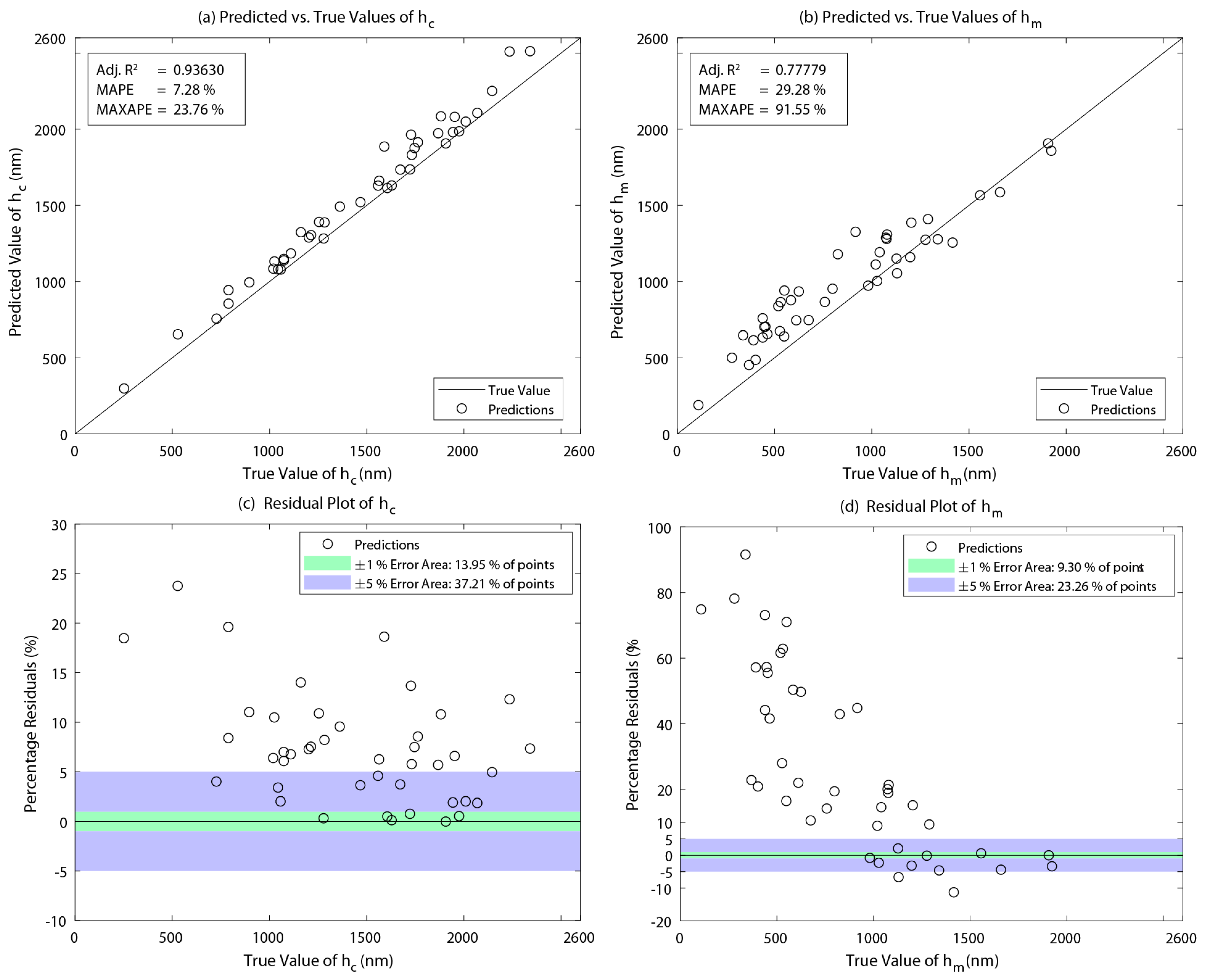
| ARD-RBF | 0.9420 | 4.65% | 49.15% | 0.8857 | 36.28% | 566.52% | |
| RQ | 0.9969 | 1.06% | 8.36% | 0.9927 | 5.38% | 30.63% | |
| 0.9993 | 0.47% | 5.98% | 0.9974 | 2.11% | 11.89% | ||
| ARD-Matern | 0.9968 | 0.87% | 20.90% | 0.9882 | 6.84% | 239.95% | |
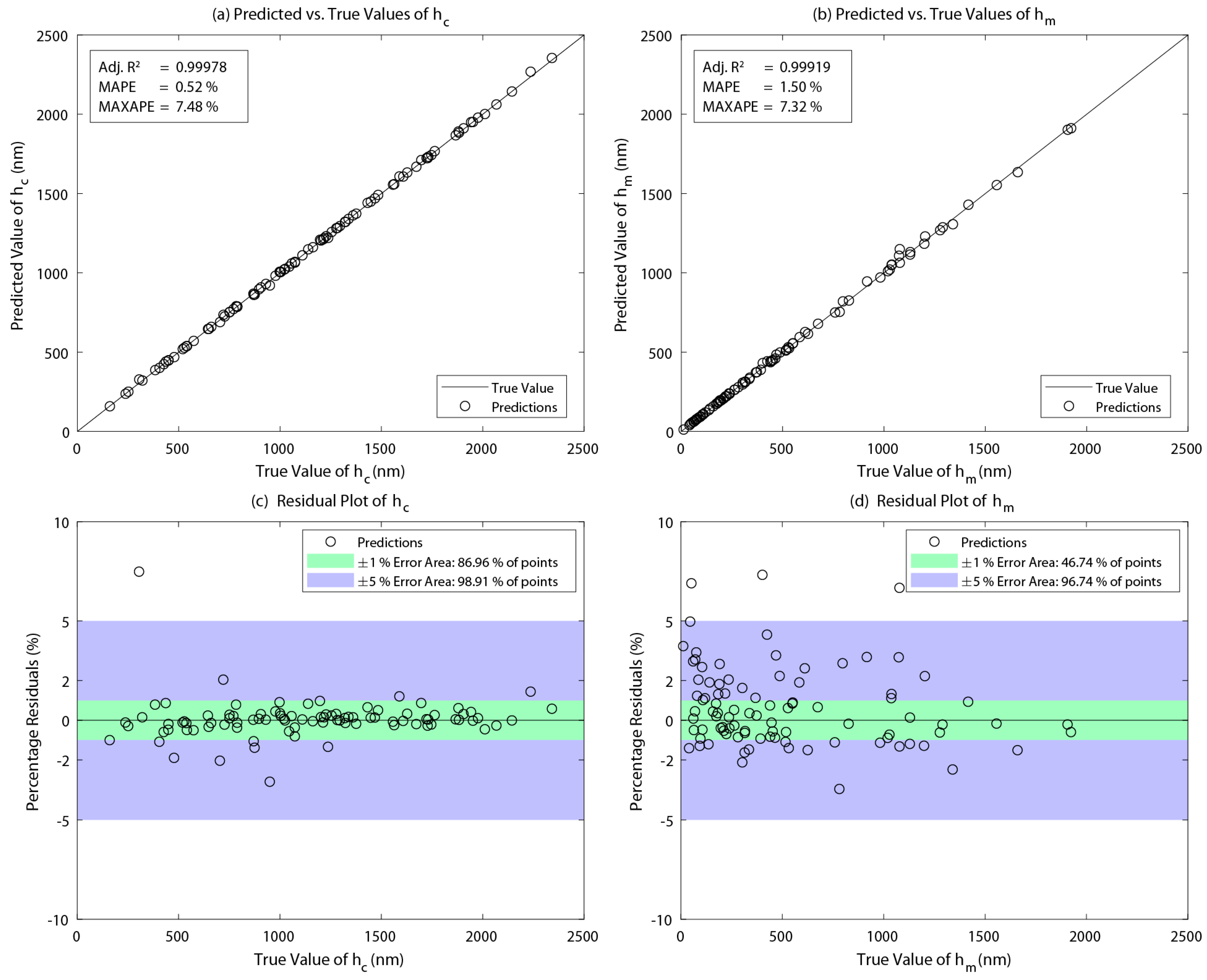
| 0.9998 | 0.52% | 7.48% | 0.9992 | 1.50% | 7.32% | ||
Disclaimer/Publisher’s Note: The statements, opinions and data contained in all publications are solely those of the individual author(s) and contributor(s) and not of MDPI and/or the editor(s). MDPI and/or the editor(s) disclaim responsibility for any injury to people or property resulting from any ideas, methods, instructions or products referred to in the content. |
© 2023 by the authors. Licensee MDPI, Basel, Switzerland. This article is an open access article distributed under the terms and conditions of the Creative Commons Attribution (CC BY) license (https://creativecommons.org/licenses/by/4.0/).
Share and Cite
Issa, J.; El Hajj, A.; Vergne, P.; Habchi, W. Machine Learning for Film Thickness Prediction in Elastohydrodynamic Lubricated Elliptical Contacts. Lubricants 2023, 11, 497. https://doi.org/10.3390/lubricants11120497
Issa J, El Hajj A, Vergne P, Habchi W. Machine Learning for Film Thickness Prediction in Elastohydrodynamic Lubricated Elliptical Contacts. Lubricants. 2023; 11(12):497. https://doi.org/10.3390/lubricants11120497
Chicago/Turabian StyleIssa, Joe, Alain El Hajj, Philippe Vergne, and Wassim Habchi. 2023. "Machine Learning for Film Thickness Prediction in Elastohydrodynamic Lubricated Elliptical Contacts" Lubricants 11, no. 12: 497. https://doi.org/10.3390/lubricants11120497
APA StyleIssa, J., El Hajj, A., Vergne, P., & Habchi, W. (2023). Machine Learning for Film Thickness Prediction in Elastohydrodynamic Lubricated Elliptical Contacts. Lubricants, 11(12), 497. https://doi.org/10.3390/lubricants11120497