Method for On-Line Remaining Useful Life and Wear Prediction for Adjustable Journal Bearings Utilizing a Combination of Physics-Based and Data-Driven Models: A Numerical Investigation

Abstract

RUL (remaining useful life) estimation is one of the main functions of the predictive analytics systems for rotary machines. Data-driven models based on large amounts of multisensory measurements data are usually utilized for this purpose. The use of adjustable bearings, on the one hand, improves a machine’s performance. On the other hand, it requires considering the additional variability in the bearing parameters in order to obtain adequate RUL estimates. The present study proposes a hybrid approach to such prediction models involving the joint use of physics-based models of adjustable bearings and data-driven models for fast on-line prediction of their parameters. The approach provides a rather simple way of considering the variability of the properties caused by the control systems. It has been tested on highly loaded locomotive traction motor axle bearings for consideration and prediction of their wear and RUL. The proposed adjustable design of the bearings includes temperature control, resulting in an increase in their expected service life. The initial study of the system was implemented with a physics-based model using Archard’s law and Reynolds equation and considering load and thermal factors for wear rate calculation. The dataset generated by this model is used to train an ANN for high-speed on-line bearing RUL and wear prediction. The results show good qualitative and quantitative agreement with the statistics of operation of traction motor axle bearings. A number of recommendations for further improving the quality of predicting the parameters of active bearings are also made as a summary of the work.

1. Introduction

One of the main functions of predictive analysis systems of machines and equipment is calculation of remaining useful life (RUL) of its key components by predicting the onset of critical conditions or defects. The approach to solving such problems is usually based on the processing of a large amount of data on the actual system states received from multiple sensors [1,2,3,4,5,6]. In addition, physics-based models of certain units and elements can be additionally introduced into the analysis process to improve the prediction accuracy [7,8,9,10].

Achieving the limit wear value is often considered as a criterion of the end of the service life of sliding bearings operating in various friction modes, especially in critical equipment. Wear can strongly influence the dynamic behavior of the rotor, both improving it at small wear values [11] and worsening it at higher values, including revealing sub- and super-harmonics [12] and decreasing critical speed and stability [13,14].

Direct measuring of the wear parameters can often be hampered due to the difficulty of accessing the installed bearings in the machine. In such cases, indirect methods are used to estimate the wear, e.g., based on the analysis of the system’s frequency response [15,16,17], and the shaft position in the bearing [18]. An alternative approach utilizes models of wear processes in bearings [19,20,21]. Calculations in such models are based on sensors measurements of the key factors influencing the wear intensity. Knowing the actual bearing wear value is a key factor in determining its RUL when considering this parameter.

Most of the described approaches to equipment RUL prediction are based on processing of significant amounts of equipment operational data under typical operating conditions [22,23,24]. Increasing the accuracy of bearings RUL prediction is the subject of many works proposing the new techniques of collecting, preparing, processing. and post-processing such data [2,25,26,27]. The new methods also address the typical problems in this area, namely the limited amount and quality of the data [28].

Adjustable design of sliding bearings is the additional challenge to their RUL prediction because the impact of control systems significantly influences the rotor system operation, including bearings degradation processes. It affects the complex of its tribological, dynamic, and integral parameters [29,30,31,32] as well as the wear parameters. Thus, the impact of controllers can even be considered as an additional uncertainty source in the system.

The adjustable design of sliding bearings can be an alternative or an addition to conventional methods of increasing their life, such as applying polymer [33] and mineral [34] coatings or implementing the rubber design [35]. However, the effect of variability of adjustable bearing properties on their expected service life is poorly assessed in studies. In [36], the reduction of wear in crankshaft bearings is claimed due to the active lubrication system, but no particular results with an analysis of the change in the life are given. In [37], the bearing life is maximized using a statistical wear model, but the considered bearings have no adjustable properties, only the parametric optimization is performed.

The work presents a novel method for the synthesis of a high-speed system for predicting the RUL and wear of friction units, namely for journal bearings operating under a range of lubrication conditions from hydrodynamic to boundary. The method is based on a principle that implies the combination of physics-based and data-driven system models. The principle has become more popular in recent years and shows outstanding results in prediction wear [38], various faults in rolling bearing [39], fatigue life [40], as well as in many other applications [41,42]. The proposed approach assumes utilizing the verified physics-based bearing models for generating the data on the predicted parameters and their subsequent use for synthesis of high-speed ANN-based prediction models. The most significant contribution of the work is the adaptation of this approach both for conventional and adjustable sliding bearings. The resulting data-driven predictive models belong to the so-called physics-informed systems and allow a wide range of tribological characteristics of bearings, including the control system in the case of their adjustable design, to be taken into account.

The implementation of the approach is demonstrated for the case of locomotive traction motor axle bearings with adjustable temperature in the friction zone. The synthesized high-speed ANN-based model is used during the bearing operation for online prediction of the wear rate and RUL values. The model utilizes insignificant computing resources and available technological information from a limited number of sensors on board. Finally, the recommendations are given on adaptation of the presented method to other configurations of rotor-bearing systems and on possible ways of improving the prediction accuracy.

2. Materials and Methods

2.1. Subject Description

Wear monitoring and increasing the service life are the actual tasks for traction motor axle bearings (TMAB) of locomotives. They provide the second fulcrum for the traction motor, and they ensure the parallelism of axes of the wheelset and the armature shaft of the traction motor, which is necessary for the correct operation of the traction transmission. The design and the arrangement of TMAB units is shown in Figure 1. TMABs usually operate under changing temperature and load conditions. Directly measuring the wear parameters of TMABs is difficult because they are located inside the traction transmission unit. However, their timely replacement is critical due to safety reasons.

A TMAB consists of liners (1 and 2) and axle boxes (3), with constant lubricant level in them. The inner surface of the liners is filled with B16 ISO 4383-91 babbitt. The liners are fastened in the frame with dowels (4). The windows for supplying the lubricant to the friction zone are placed in the liners facing. The lubricant is supplied from the chamber (5) in the axle box through woolen wicks (6).

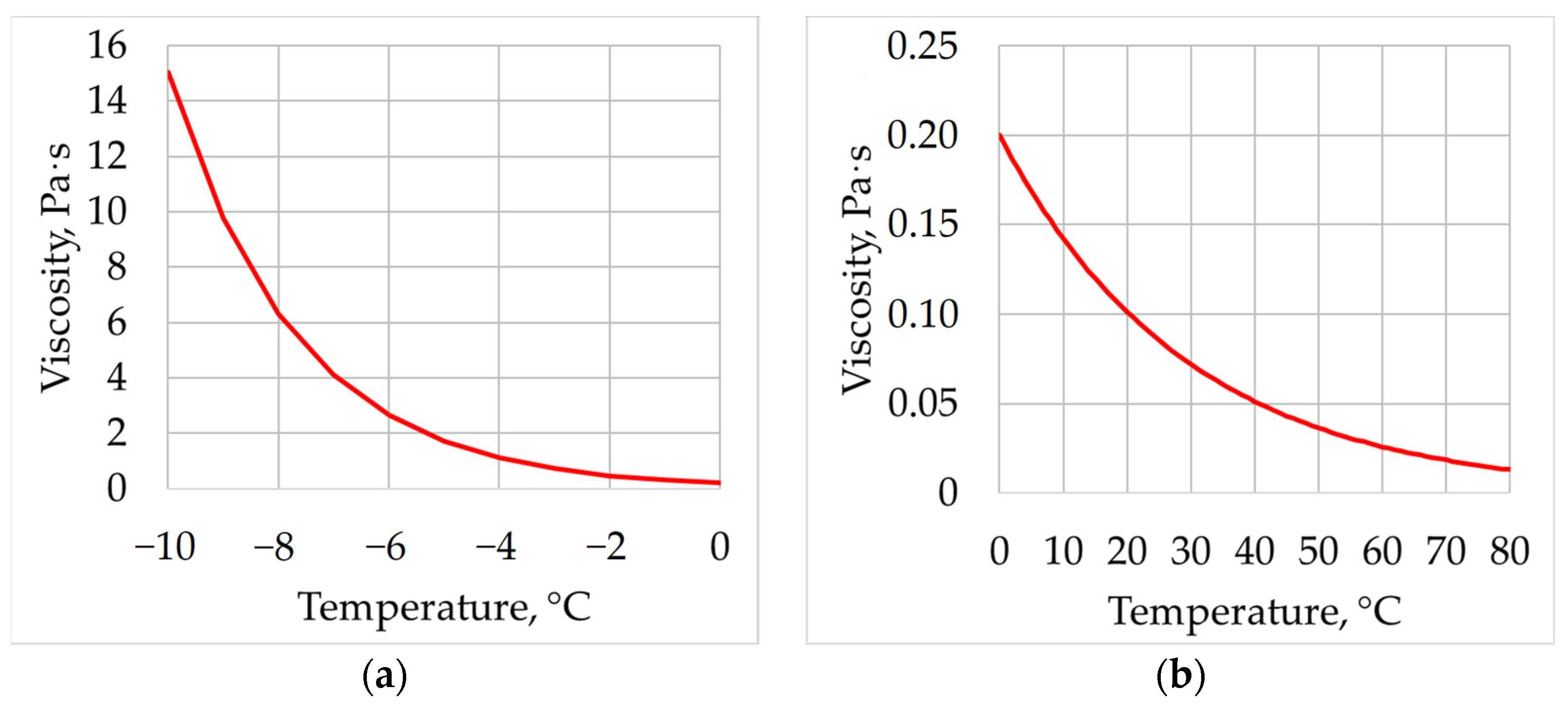
Axial oil type L GOST 610-2017 is used as the main lubricant for the summer operating conditions. According to the technical data, the temperature in TMABs can vary from −10 to +80 °C during the locomotive motion. The oil dynamic viscosity varies at these conditions from 15 to 0.01 Pa·s, that is, by more than three orders of magnitude, as shown in Figure 2.

A wide range of changes in the oil dynamic viscosity depending on the temperature makes it possible to use this effect for a controlled impact on the tribological processes in the bearing with minor design changes. It is proposed to introduce cooling elements (7) and a temperature sensor (8) into the bearing unit near the mostly loaded zone that is also primarily worn, as schematically shown in Figure 1. Peltier modules or components of the locomotive conditioning system can be used as the thermal elements; however, the specific design of the cooling system is not the subject of this article. In this work, only a general principle of adjusting a bearing parameter for modifying the friction mode is considered to show how the presented method is applied to adjustable bearings.

2.2. Wear Model

The Archard’s wear model [43,44,45,46] and Fleischer’s energetic wear model [45,46,47,48] are most commonly used to calculate the wear of various materials. They usually demonstrate the comparable accuracy [45]. However, the Archard’s wear model is more common, and more theoretical and experimental data are presented for it, so it was chosen for the physical-based wear model in this study.

Initially, the wear process is characterized by linear, volumetric, or mass wear rate. According to [49], volumetric wear rate is calculated using the Archard’s equation:

$$V=\frac{K{S}_{n}P}{HB},$$

(1)

where K is the dimensionless wear coefficient; S_n is the friction path for 1 h, m/h; P is the total load, N; and HB is the hardness of the wear material, MPa.

The linear wear intensity is determined by the ratio of volumetric wear to the contact area A_k, m²:

$$I_h=\frac{K{S}_{n}P}{HB{A}_k}.$$

(2)

The total linear wear d₀ of the bearing surface is determined by the ratio:

$$d_0={\displaystyle \underset{0}{\overset{t}{\int }}{I}_{h}dt}.$$

(3)

The main difficulty in applying the Archard’s Equation (1) is to determine the actual wear coefficients for different friction modes. As a rule, such data are presented for special cases, for various pairs of materials, loading, and lubrication conditions [50]. The estimated values of wear coefficients were obtained on the basis of data for similar materials from [44,51,52,53,54] for this study: for the boundary friction, K is of 3 × 10⁻⁸; for the fluid friction, K is of 3 × 10⁻¹⁰; and for the mixed friction, K value varies depending on the λ parameter, as shown in Figure 3.

The mentioned λ coefficient reflects the current lubrication mode [55]:

$$\lambda =\frac{h_{\min }}{R_z^b+R_z^j},$$

(4)

where h_min is the minimum radial clearance between the TMAB bushing and the axle journal; R_z^b is the roughness of the working surface of the TMAB liners; and R_z^j is the roughness of the axle journal.

The λ value characterizes the current type of lubrication: boundary at λ < 1 mixed at 1 < λ < 3 and the hydrodynamic at λ > 3.

The practical application of the described approach requires experimental refinement of the coefficient values. However, it should be noted that such a refinement will not have a qualitative impact on the developed models and will not require any significant changes to the presented approach and methods.

Thus, the boundary friction in the considered TMAB occurs at h_min < 14.3 μm, the mixed friction at 14.3 μm < h_min < 42.9 μm, and the hydrodynamic lubrication occurs at h_min > 42.9 μm. These values can be recalculated to the values of the relative eccentricity of the journal position, corresponding to the boundaries between the friction modes. Thus, the boundary friction is replaced by the mixed at e₁ = 0.956, and the hydrodynamic lubrication regime begins at e₂ = 0.868.

The position of the journal in the TMAB depends on the ratio of the external force and the load capacity of the lubricant film under current conditions. The external force is determined mostly by the traction motor mass, as well as the radial and circumferential forces of the gearing. The resulting diagram of the relationship of the loads and friction modes is shown in Figure 4. The details of the calculation are omitted because they are not the subject of this study. In the general case, the calculation method may vary on the basis of the structure and principle of operation of the system under consideration during implementation of the overall approach presented in this paper. However, a relation representing the dependence of friction modes on the generalized load indicators comparable to that shown in Figure 4 is required nonetheless.

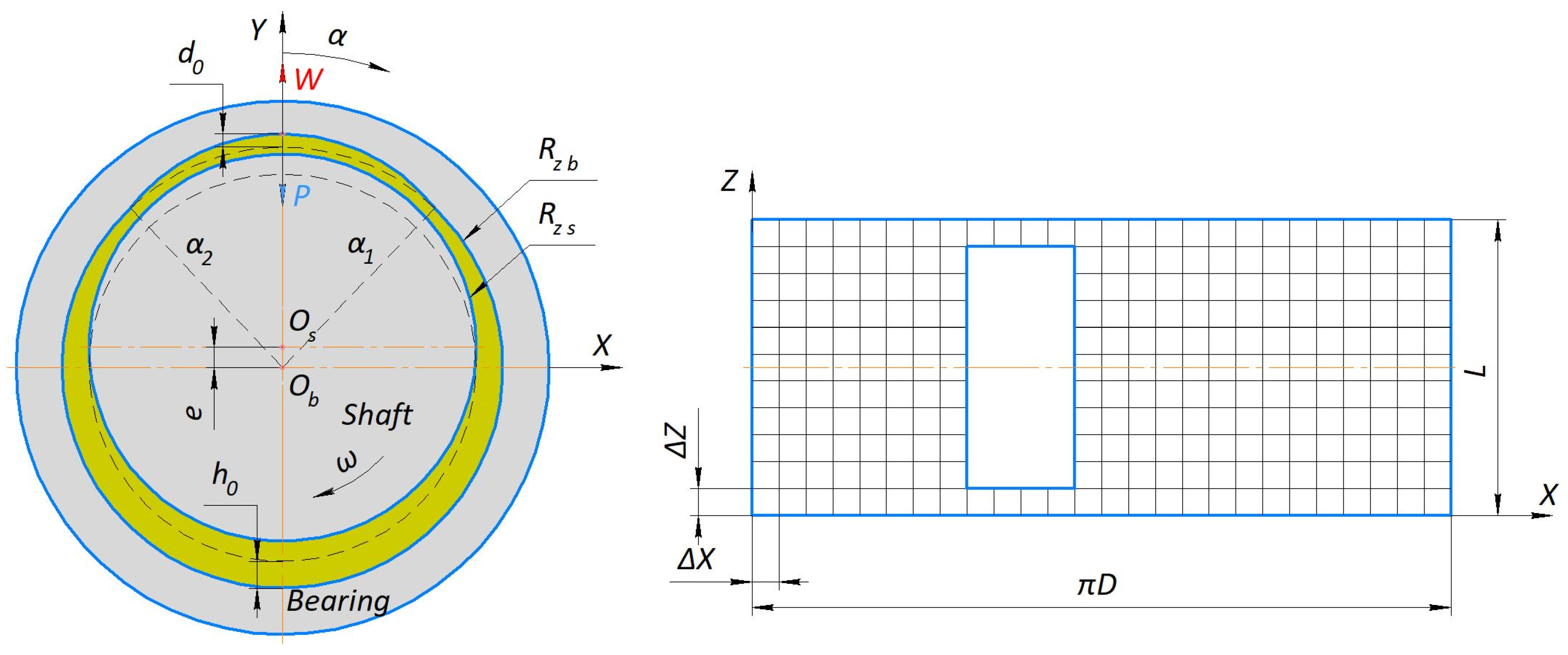
The TMAB calculation scheme is shown in Figure 5. It includes the geometric parameters of the wear zone and a finite-difference grid placed over the bearing surface for the further force calculation.

The load capacity of a hydrodynamic bearing is calculated by solving the Reynolds equation for the two-dimensional incompressible fluid flow numerically [56]:

$$\frac{\partial }{\partial x}\left[h^3\frac{\partial p}{\partial x}\right]+\frac{\partial }{\partial z}\left[h^3\frac{\partial p}{\partial z}\right]=6\mu \frac{\partial }{\partial x}\left(V_{1}h\right)-12\mu V_2,$$

(5)

where V₁ and V₂ are the components of the lubricant flow velocity in the fluid film in the circumferential and radial directions, correspondingly; μ is the lubricant dynamic viscosity; and h is the radial clearance.

The clearance distribution along the circumferential coordinate of the bearing for a certain eccentric position of the shaft in the bearing is defined as:

$$h_1\left(\alpha \right)=h_0-X\sin \left(\alpha \right)-Y\cos \left(\alpha \right),$$

(6)

where X and Y are the Cartesian coordinates of the journal center.

The resulting wear profile is described by the following equation:

$$d\left(\alpha \right)=d_0-h_0\left(1+\cos \left(\alpha \right)\right).$$

(7)

The resulting clearance function of a worn bearing is a superposition of (6) and (7):

$$h\left(\alpha \right)=\{\begin{array}{l}{h}_1\left(\alpha \right),{\alpha }_1<\alpha <{\alpha }_2,\\ h_1\left(\alpha \right)+d\left(\alpha \right),0\le \alpha \le {\alpha }_1\vee {\alpha }_2\le \alpha \le 2\pi ,\end{array}$$

(8)

where α₁ and α₂ are the limits of the worn area along the angular coordinate α.

Equation (8) is solved together with the numerical solution of the Reynolds Equation (5) using the finite difference method, resulting in the pressure distribution p in the bearing. The bearing forces R_x and R_y are calculated by integration of p over the bearing surface:

$$R_X={\displaystyle \underset{0}{\overset{L}{\int }}{\displaystyle \underset{0}{\overset{\pi D}{\int }}p\cdot \cos \left(\frac{x}{r_{TMAB}}\right)dxdz;}}{R}_Y={\displaystyle \underset{0}{\overset{L}{\int }}{\displaystyle \underset{0}{\overset{\pi D}{\int }}p\cdot \sin \left(\frac{x}{r_{TMAB}}\right)dxdz}}.$$

(9)

Hence, the bearing load capacity:

$$W=\sqrt{R_X^2+R_Y^2}.$$

(10)

The relationship of the bearing force factors, including the load capacity, with friction modes, is also shown in the diagram in Figure 4.

Additionally, the temperature rise and the corresponding change in oil viscosity due to friction in the bearing is calculated with the equation [57]:

$$T=\frac{3}{4}\frac{{\mu }_0{v}_{sl}^2}{k_f}+T_0,$$

(11)

where T₀ is the initial (ambient) temperature at which the dynamic viscosity of the oil is of µ₀; k_f is the thermal conductivity of the lubricant, W·m⁻¹K⁻¹: for most oils, k_f is of 0.14 W·m⁻¹K⁻¹. v_sl is the sliding speed v_sl = ωd, m/s, where ω is the angular journal velocity, rad/s, and d is the journal diameter, m.

2.3. Operating Conditions

The wear intensity of a sliding bearing significantly depends on the ratio of the current force factors. These factors determine the relative position of the journal and the bearing surfaces and, as a result, the current friction mode (Figure 3). The current journal rotation speed (proportional to the translational locomotive speed) and the temperature in the bearing can be highlighted, among other operational parameters, as those most influencing the wear rate. They can be considered as the independent variables in the wear model that determine the tribological modes of operation of the rotor-bearing system.

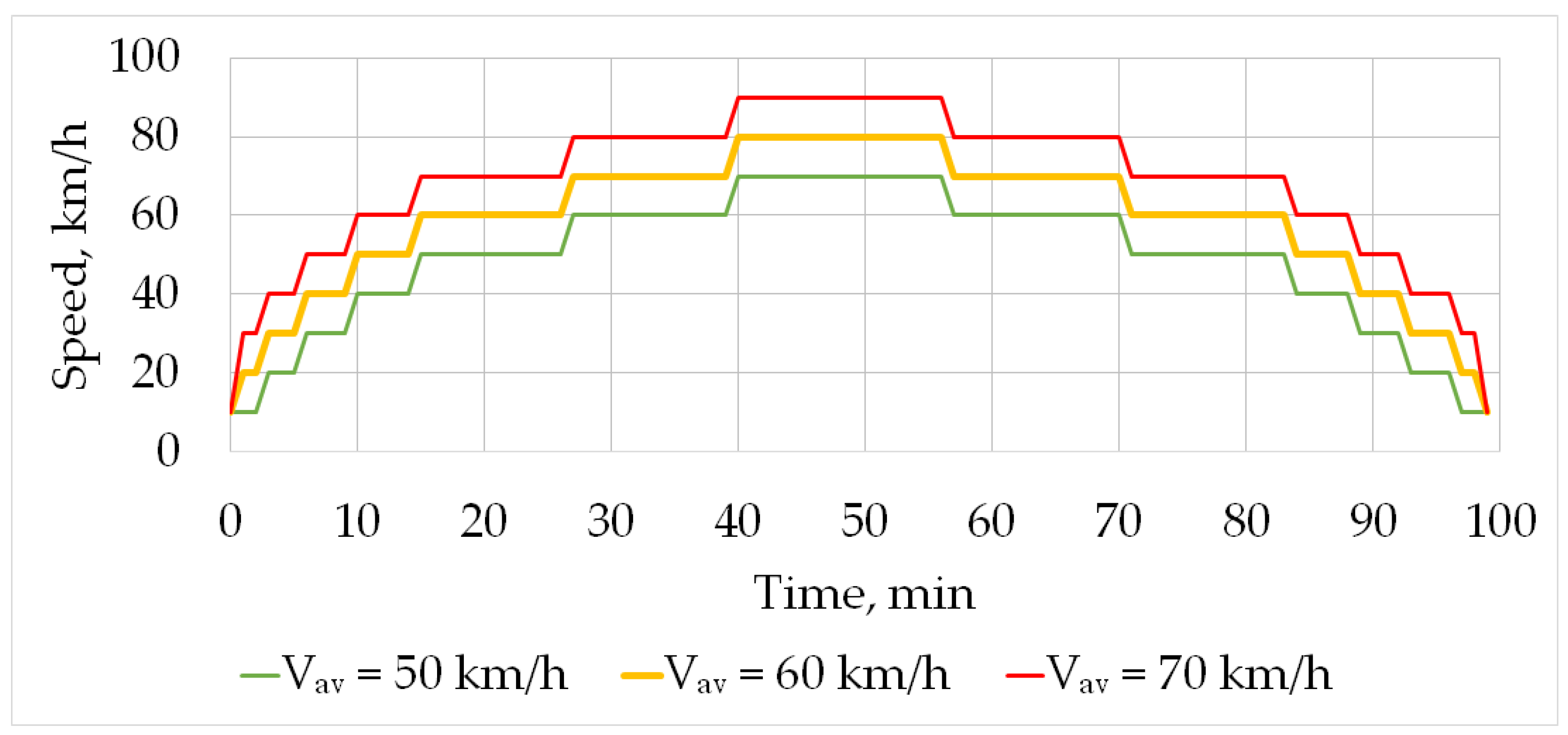
The actual operating conditions of the considered system as part of the locomotive are continually changing in a sporadic manner. Therefore, the numerical tests in this study utilized the normalized load models considering operation in temperate climate conditions. The basic ambient temperature was set at 20 degrees. The average speed distribution diagram is based on the statistical data on locomotive speeds over a long period of time and is shown in Figure 6.

All tests were carried out for a seamless railroad track to simplify the interpretation of the results. In such conditions, the load is determined only by the speed of the locomotive. In the following numerical tests, unless otherwise indicated, the speed diagram with the average speeds of V_av = 60 km/h, shown in Figure 6, was used. Such a load was applied repeatedly to the system during the simulation of the operating life of the bearing until the wear limit was reached. The linear wear depth of d₀ = 500 µm was set as the limit value for the TMAB according to the current maintenance regulations.

Table 1. The main TMAB parameters.

Parameter	Notation	Value	Unit
Diameter of bearing	D	0.20575	m
Length of bearing	L	0.275	m
Diameter of journal	d	0.20496	m
Clearance	h0	395	μm
Maximum wear depth	d0	500	μm
Roughness of bearing	Rzb	8	μm
Roughness of journal	Rzj	6.3	μm
Material of bearing	-	Steel OS	-
Material of journal	-	Babbitt B16	-
Wear coefficient	K	3 × 10−10–3 × 10−8	-
Maximum external load	P	48	kN
Maximum rotational speed	ω	44.4	rad/s

shows the main parameters of the considered TMAB.

2.4. General Algorithm of RUL and Wear calculation

The process of wear calculation using the physics-based model presented in Section 2.2 requires a significant amount of computation. Numerical solution of the Reynolds Equation (5) with the appropriate accuracy is the most calculation-consuming part of the simulation. In addition, the operating conditions vary continuously during the operation of the bearing within a certain range of conditions. It is proposed to reduce the required amount of calculation for predicting the wear rate and RUL during the bearing service life by moving towards data-driven models. The required data for training such models using machine learning methods should be obtained once from the physics-based model for a full range of operating conditions.

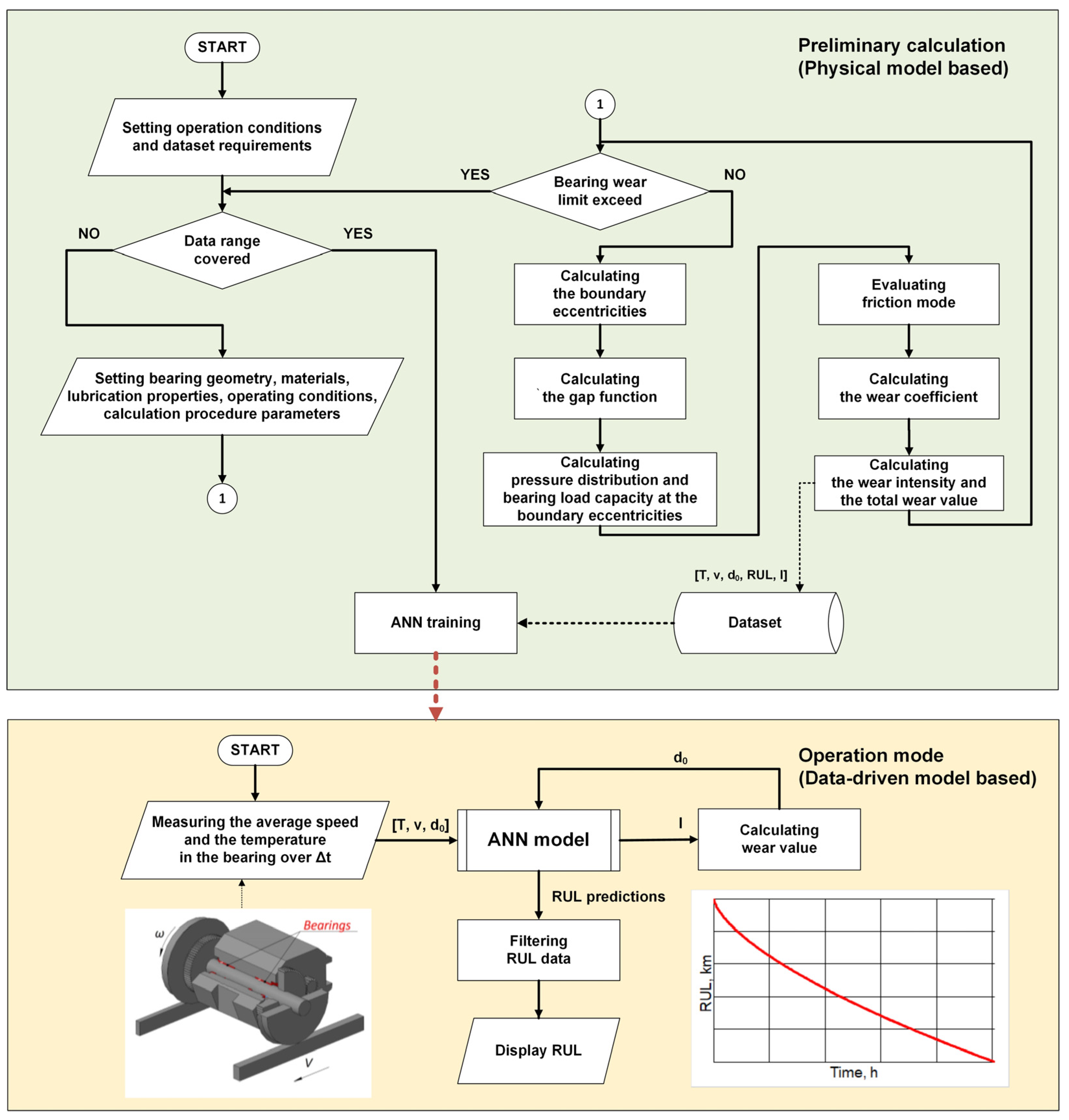
The physics-based model in the proposed approach is used to generate complete data on the wear process and RUL value for various combinations of independent factors influencing them. These include primarily the generalized parameters describing the external loads, as well as the parameters characterizing the bearing’s ability to withstand such loads. The latter include the parameters that determine the bearing load capacity, both structural and controllable, in the case of adjustable solutions. In the considered case of TMAB, the mentioned factors are represented by a single parameter, namely the temperature of the lubricant in the friction zone, which also determines the lubricant viscosity. In addition, the current linear wear value d₀ is among the influencing factors, since it changes the contact area A and wear intensity I according to Equation (2). Thus, a dataset consisting of multiple variations of the set of 5 parameters [v T d₀ RUL I] should be generated to create a data-driven model based on machine learning. The first three parameters [v T d₀] are the independent variables. Their values should cover the full range of the system operating conditions and vary with a certain step within it. The last two parameters [RUL I] are to be predicted by the data-driven model on the basis of the values of the independent variables. The flow chart diagram illustrating the proposed approach and method is shown in Figure 7.

Figure 7 shows that the proposed method includes two main stages. The first stage involves the creation of a physics-based wear model, setting the required range of the operating conditions to be simulated, and generating a dataset. The stage ends with the training of a data-driven model, using an ANN or any other machine learning method providing the necessary prediction accuracy. The second stage implies the practical operation of the developed data-driven model. The necessary parameters are measured directly or indirectly using sensors during the equipment operation. The obtained data are transferred to the input of the ANN model. Finally, the wear parameters are calculated and recorded on the basis of its outputs, and the RUL value is continuously evaluated and displayed, if required.

In Section 3, the validity and implementation of the proposed method will be illustrated by the results of numerical calculations. Among them, an analysis of the influence of the mentioned factors on the bearing wear process will be carried out, highlighting the most significant relationships. The process and results of synthesis of an ANN-based data-driven model, as well as the analysis of the prediction accuracy, will be shown. Finally, an example of calculating the wear parameters and RUL during the simulation of one bearing life cycle will be presented.

3. Results and Discussion

3.1. Wear Calculation

3.1.1. Passive Bearings

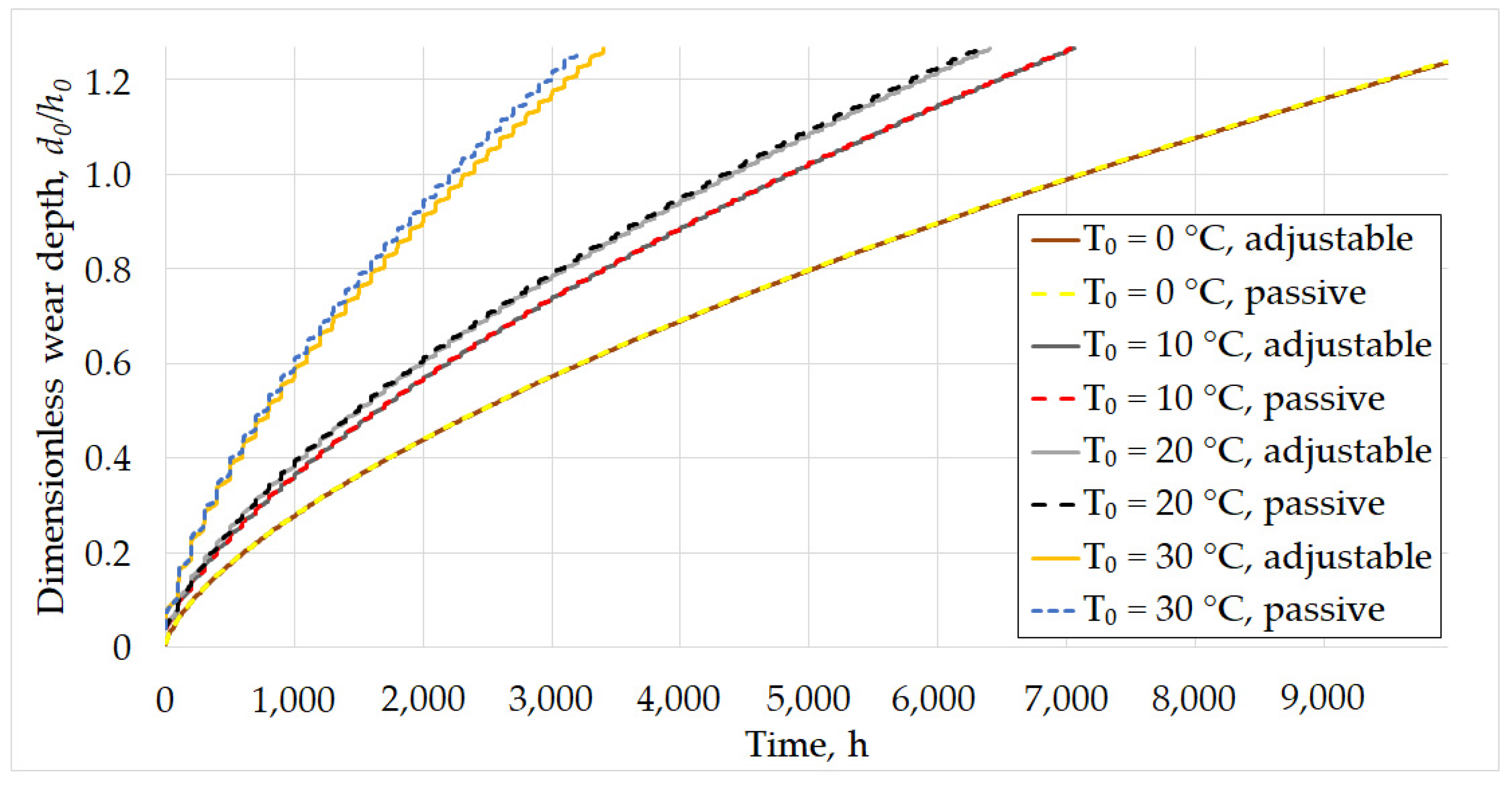
The simulation results for a passive bearing wear at various ambient temperatures are shown in Figure 8. These results consider the effect of an additional temperature rise in the friction zone, described by Equation (11).

The obtained wear curves are qualitatively similar to the theoretical and experimental [43,44,58,59] results of other authors. In addition, the estimated service life values of several hundred thousand kilometers (2–10 thousand hours at an average speed of 60 km/h) are in good agreement with the statistical data on typical TMAB service life [60]. This proves the qualitative adequacy of the developed wear model.

Figure 8 demonstrates that the most intense wear occurs at higher ambient temperatures. As the lubricant temperature rises, its viscosity and the bearing load capacity decrease. The bearing operates longer under mixed and boundary lubrication conditions at lower speed values, which leads to faster degradation. In addition, the highest wear rate is observed for a new unworn bearing, and then the wear rate slowly decreases. The reason for this is the small contact area between the rotor and the unworn bearing, which means the maximum pressure in the friction zone and the fastest wear. Further, as the wear depth increases, the contact area also increases and the wear rate decreases.

As noted above, another factor that significantly affects the friction mode is the journal rotation speed. Figure 9 shows wear curves for the various locomotive speed diagrams shown in Figure 6.

The expected bearing service life increases with an increase in the average speed. At higher rotation speed, the system operates longer in the hydrodynamic lubrication mode, which minimizes the wear. In addition, the expected bearing service life varies unevenly with a change in the average speed. In particular, in the simulated cases, it increases by 17% with the increase in the average speed of 10 km/h, and decreases by 41% with the speed decrease of 10 km/h. Such non-uniformity reflects the dependence of the wear coefficient K on the friction mode. It almost does not change at hydrodynamic lubrication, and it increases significantly when moving towards boundary friction, as shown in Figure 3.

3.1.2. Adjustable Bearings

As shown in Figure 8, the service life of the TMAB strongly depends on the lubricant temperature in the friction zone. The actual temperature in the TMAB is determined by two factors, the ambient temperature and the speed of the locomotive, see Equation (11). Cooling thermal elements were introduced into the proposed adjustable TMAB design in order to compensate for the additional heating due to friction and decrease the lubricant temperature in general (see Figure 1). In addition, the following assumptions were made: (1) the temperature varies insignificantly within the wear region of the adjustable bearing, regardless of operation of the cooling elements; (2) the feedback sensors provide the representative data regarding the bearing and lubricant temperature, and they are equal within and near the wear region; and (3) the control system provides stable behavior and insignificant deviations of the controlled temperature.

The minimum achievable temperature in the bearing is limited by the cooling capacity of the thermal elements used. Thus, it is also assumed that the temperature rise due to friction, in accordance with Equation (11), can be fully compensated in the adjustable bearing and that the cooling capacity is sufficient to maintain the temperature in the bearing lower than the ambient. Figure 10 shows the comparison of wear process in the passive bearing and in the adjustable bearing, with the temperature stabilized at the ambient level.

As can be seen from the results, simple temperature stabilization at the ambient level almost does not increase the expected TMAB service life compared with the passive design. A small difference of 3% in RUL is observed only at the temperature of approximately 0 °C. A significant increase in TMAB service life can be achieved only if the temperature in the friction zone is set lower than the ambient. This is due to strong non-linear rise in the lubricant viscosity, as shown in Figure 2. The bearing load capacity and, consequently, its resistance to excessive wear under non-hydrodynamic lubrication linearly depend on the lubricant viscosity, as seen from Equation (5). So, a strong increase in the lubricant viscosity should be achieved to obtain a significant increase in the bearing life.

A more complete analysis of the influence of the controlled temperature in the TMAB on its service life is shown in Figure 11. The presented results summarize the previously drawn conclusions on the influence of temperature and loads on the wear process. In these results, the temperature in the adjustable bearing is maintained at the ambient level to make the dependencies clearer. As can be seen, the combination of conditions, together with an exponential increase in the lubricant viscosity with a decrease in temperature in the bearing, gives a significant increase in the resource, and vice versa. In addition, the dependencies in Figure 11 can be used for selecting the rational cooling capacity of the bearing cooling system.

3.2. Prediction of RUL and Wear Rate

As shown above, the dependence of the expected TMAB life on the speed and temperature is non-linear. The form of such dependence for the system under consideration is shown in Figure 12. The values of the expected life (RUL) were calculated for the fixed values of speed and the stabilized temperature values in the friction zone. The results in Figure 12 reflect the same dependencies as in Figure 11, but the form of their representation makes it easier to estimate the wear rate for a given configuration of the system parameters, speed, and temperature.

The linear wear rate decreases with an increase in the wear depth d₀ due to the increase in the contact area A_k, which can be observed in Figure 8, Figure 9, Figure 10, Figure 11 and Figure 12. The obtained results confirm that the RUL value and the instantaneous wear intensity I strongly depend on three parameters: the current speed v, the current temperature in the bearing T, and the current wear D₀. Thus, the dataset for training a predictive ANN-based model should include the calculated values of [RUL I] for various combinations of independent parameters [v T d₀].

In order to test the proposed method, a dataset with the following parameters was generated with the physics-based model described above for a certain range of independent parameters. The speed varied from 0 to 100 km/h with a step of 10 km/h; temperature varied from 0 to 80 °C, with a step of 5 °C; and the wear value varied from 0 to 100% (500 microns), with a step of 5 microns. The wear rate value was calculated as I = Δd₀/Δt_i, and the RUL value was expressed in kilometers. Thus, the uniform parameters grid in the computational domain was chosen. The resulting dataset consisted of 230 thousand strings [v T d₀ RUL I].

It should be noted that the nature of data changes in the dataset affects the quality of training of the ANN-based model. The diagram in Figure 12 shows the presence of the region of the fastest change in RUL for each temperature and speed. Such change is associated with the transition between friction modes under the appropriate conditions. In order to improve the accuracy of data interpolation in the trained model, a grid of increased density can be applied in the corresponding regions. At the same time, it is possible to avoid an increase in the volume of initial data in other data regions.

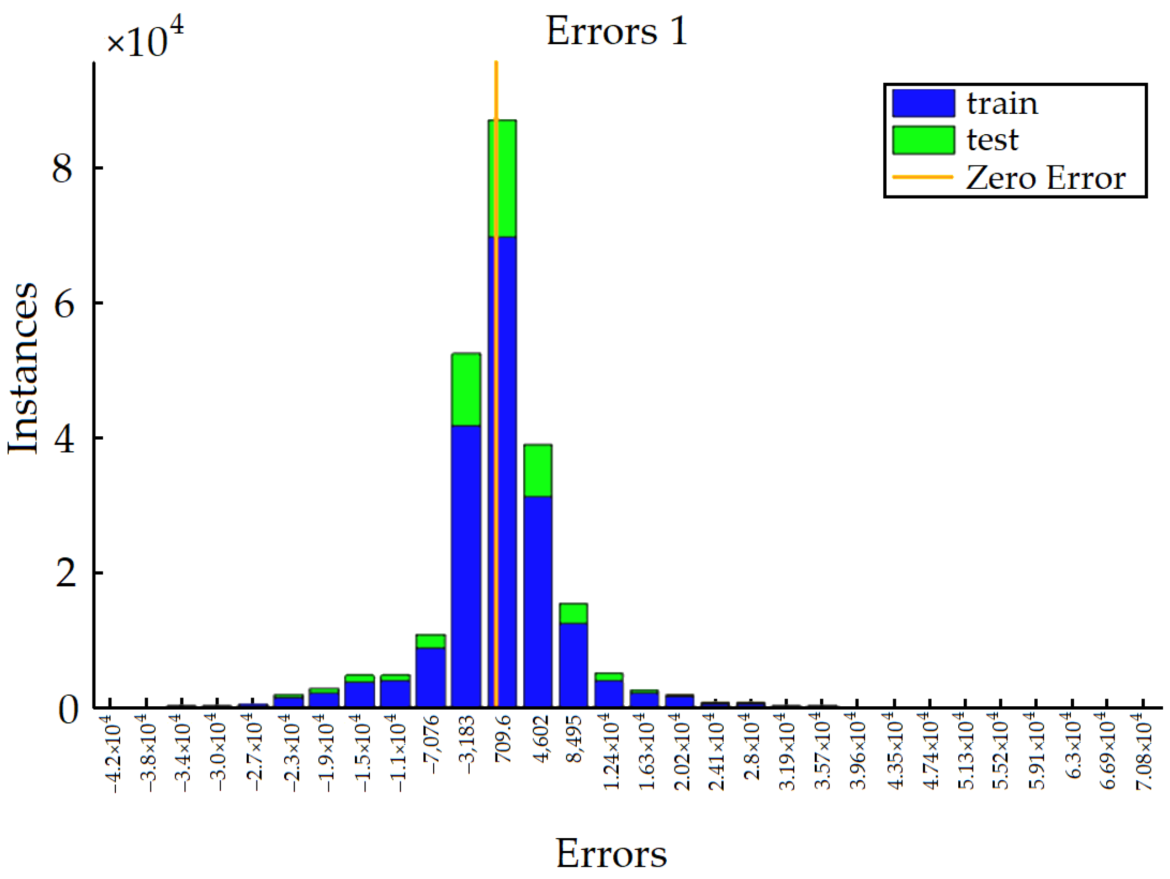
A fully connected ANN was used to solve the approximation problem. The ANN input is a vector of three values [v T d₀], and the vector [RUL I] is its output. The ANN was tuned by optimizing four hyperparameters: the size of hidden layers, the number of hidden layers, the regularization coefficient, and the learning step. The PyTorch library for the Python3 language was used to implement the model. The ANN was trained using a modification of the Adam gradient descent method to minimize the mean square loss function (MSE loss). The ReLU activation function [61] was used in the hidden layers. The input and the output values were normalized by adjusting to zero mean and unit variance. The quality of models for predictions was assessed by calculating the average and maximum relative errors for each output value. The distribution of the error value was also evaluated to assess the possibility of filtering and averaging predictions during the further use of the model. The training results with the analysis of the accuracy of predicting RUL are shown in Figure 13.

The graphs show that the RUL value error is the largest in the range of its small values, while for large RUL values, it is insignificant. The resulting prediction accuracy is acceptable given the iterative process of calculating RUL during the system operation and the close-to-normal distribution of the prediction error, as can be seen in Figure 14. The latter gives a reason for using fairly simple filtering algorithms to filter out data outliers.

A number of calculations of the bearing wear process for various speed and temperature conditions were repeated using the ANN-based model. In Figure 15, these results are compared with the similar results calculated with the physics-based model. The observed approximation error does not exceed a few percentage points in the entire computational domain, so the results provided by the models can be considered identical.

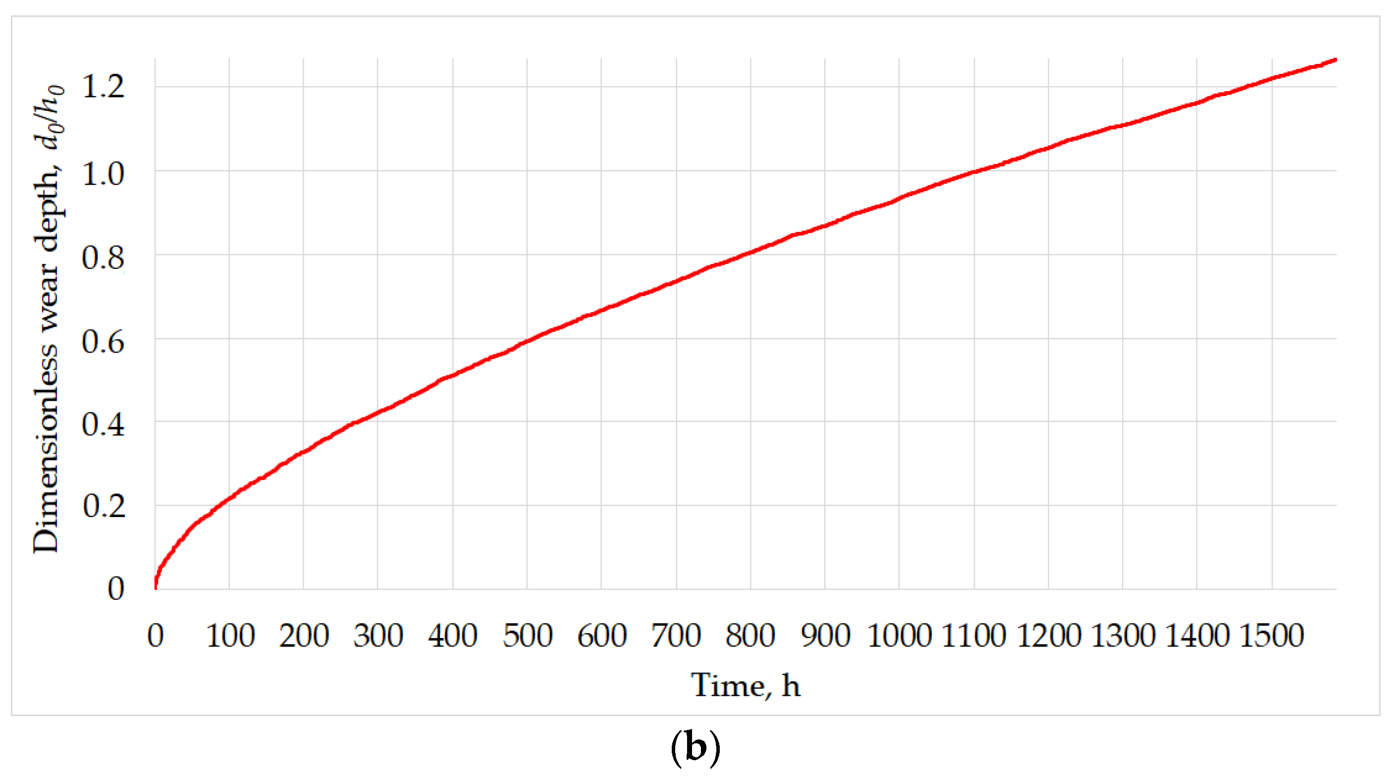
A more realistic scenario was simulated to test the resulting ANN model and the method as a whole. The movement speed varied randomly every 6 min of the simulation time, while the temperature in the friction zone of the bearing remained stabilized at 20 °C. Simulation modeling was carried out until the maximum wear was reached. The generated speed diagram and the corresponding wear diagram are shown in Figure 16.

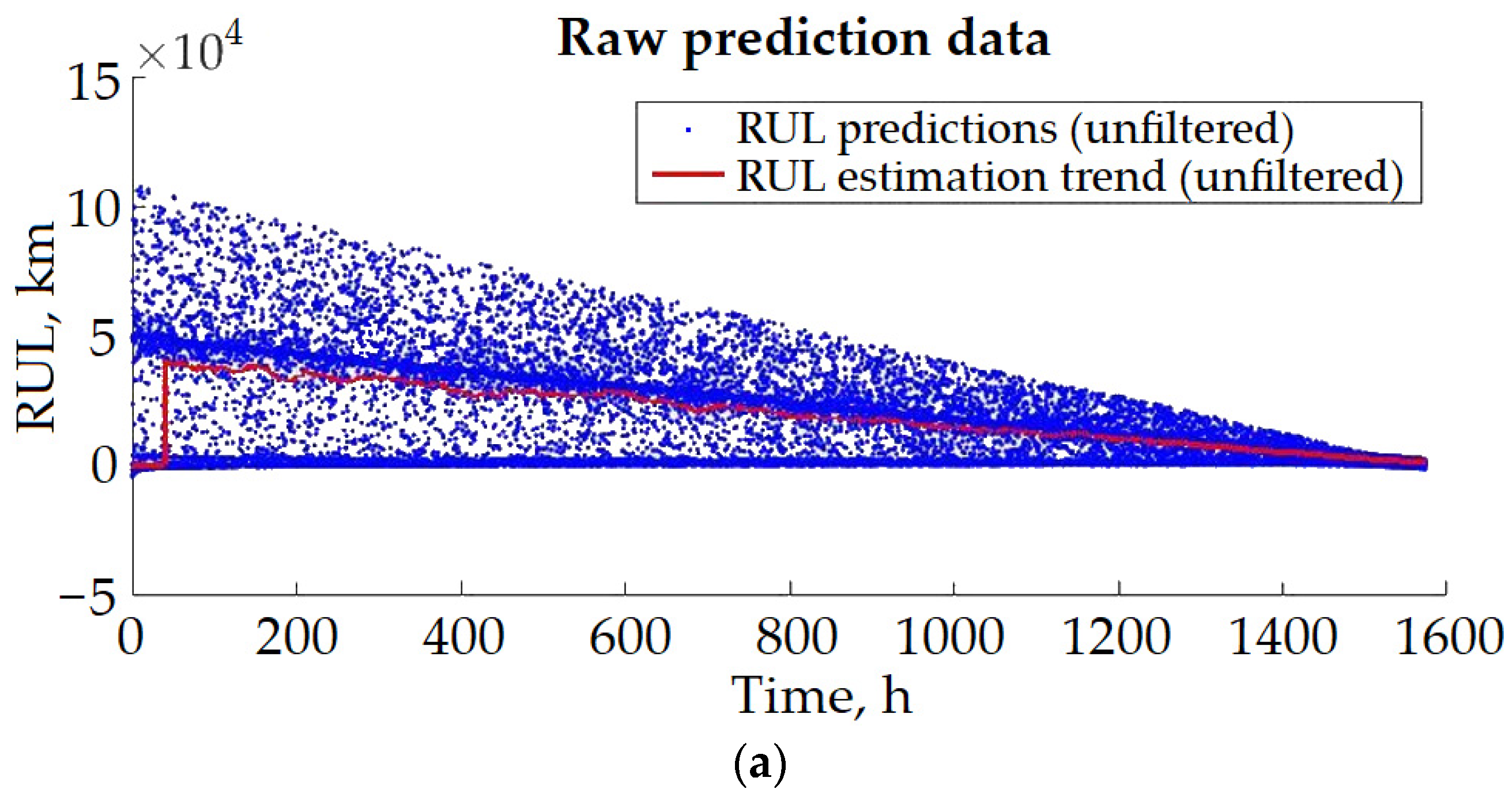
The predicted RUL values are shown in the diagram in Figure 17a. Two trends with the highest predictions density can be observed in the raw data in Figure 17a. One of them shows a realistic decrease in the RUL value over the simulation time, the other is observed in the near-zero region. Due to the significant scatter of the predicted RUL values, the data were processed using the moving average method to obtain a single and stable RUL value at each time, taking into account that the prediction error distribution is close to normal. The window size of 300 values was taken, due to which there is a delay in estimating the RUL value in the initial period of simulation for accumulating the required amount of data. As can be seen from Figure 17a, after the processing, the final RUL values turn out to be underestimated by approximately 8–10% relative to the expected value. Such a discrepancy appears to be due to the presence of the secondary trend with the predicted values around zero.

Considering the close-to-normal prediction error distribution, threshold filtering with a cutoff of 1.5 σ was applied to the raw RUL prediction data. Filtering was also implemented within a sliding window of 300 values. Data outside the 1.5 σ range were considered outliers. However, they were not removed completely, but replaced with a value of −1 to preserve the timeline continuity. When the RUL was recalculated using the moving average method, such values were not taken into account. As a result, Figure 17b shows that the RUL estimation trend based on the filtered data is in good agreement with the visual trend with the highest predictions density. The resulting trend gradually and relatively smoothly decreases and approaches zero when the wear approaches the maximum, according to the data in Figure 16. Accordingly, such RUL assessment can be used in the practical operation of TMABs in locomotives. In addition, only insignificant computing resources and memory are required for operation of the ANN-based predictive model on board.

3.3. Discussion

The presented method for online RUL prediction is based on the interaction of the physics-based and the data-driven wear models of a sliding bearing. The physics-based model provides the feasibility of a quite full account of the main physical processes in the considered system as well as their mutual influence. In the case of adjustable bearings, they also take into account the factor of the control system, which introduces additional complications and uncertainties into operation of the rotor system. They arise because the outputs of the control system depend on unpredictable environmental factors and relatively complicated control algorithms. So, analytical prediction of influence of control on wear processes is also a rather difficult task. At the same time, physics-based models of fluid film bearings often require significant computational resources. Such calculations are usually difficult to implement on board of the corresponding machines, using their monitoring and control systems. They usually have limited computational capacity, and they may be in competition with other computing tasks. Therefore, data-driven models can be utilized to reduce the required calculation amount. They usually approximate the pre-generated data on the system operation using machine learning methods. Despite approximations never being perfect in accuracy and having certain errors in the predictions, adequate estimates of the key parameters, such as the instantaneous wear rate and RUL value, can be obtained using filtering and post-processing of the prediction data.

In this paper, the proposed method is considered and numerically implemented for the case of locomotive traction motor axle bearings. They have some specific performance features that may not be typical for sliding journal bearings in other applications. Moreover, the lubricant temperature is considered as an adjustable parameter, while there is a significant variety of active control schemes in fluid film bearings. A comprehensive review of them is given, for example, in [62,63]. With that, when considering alternative systems with sliding bearings, the basics of the described approach and method can most likely be applied without fundamental changes. A brief analysis of the most possible distinctions and the possible ways of taking them into account for implementation of the presented method is given below.

• Differences in bearing loading schemes. In the considered case, the mechanical loads applied to the bearing are described mainly by the speed of the locomotive. In other applications, the sources and types of bearing loads may be more diverse. If the existing loads cannot be described by a single generalized parameter, one or more additional parameters should be introduced to the dataset. Such parameters should together give a complete assessment of the loads based either on their direct measurements or on indirect estimates using other types of sensors.
• Differences in the schemes of adjustment of the bearing parameters. As in the previous case, if the control scheme implies adjusting more than one of the independent parameters considered in the physics-based model, one or more additional generalized parameters should be introduced that reflect the magnitude of the control action. When generating a dataset, the range of change of introduced parameters should be divided into steps in the same way as described in Section 3.2.
• By analogy with points 1 and 2, in the case of any other differences, it is recommended to parameterize them, making sure that their values can be estimated using the measurement data in the system, and introducing them to the dataset among the variables that have a significant impact on the estimated parameters.

It should be noted that increasing the dataset dimensionality by supplementing it with new independent variables can complicate the task of approximating the data with acceptable accuracy. In such cases, application of more advanced machine learning algorithms and/or more advanced methods of data pre- and post-processing can be considered.

In general, the issues of the adequacy and accuracy of the results obtained with the presented model should also be noted separately. Although the results of numerical studies in this work demonstrate good qualitative agreement with the experimental data of other researchers and the general nature of the considered physical processes, as noted above, a number of significant parameters still require clarification. Therefore, it is useful to point out a number of both necessary and desirable measures that would also allow maximizing the quantitative adequacy of the results obtained with the presented models.

Experimental refinement of the dimensionless wear coefficients values for specific friction pairs is a mandatory measure. Although the nature of the dependences considered will generally remain the same in this case, the ranges of the results may be shifted, and individual quantitative estimates may also change.

The other measures that can positively affect the accuracy of the results obtained are as follows.

• Increasing approximation accuracy. The practice of applying machine learning methods shows that the choice of the methods themselves and their hyperparameters in most cases should be made individually, even including the elements of an heuristic approach. The variety of machine learning techniques gives a wide scope for tests and possible improvements. The dataset can also be optimized, including the reduction of its dimensionality, if possible, as well as adjusting the discretization step of the independent variables, including the use of adaptive grids.
• Using advanced techniques of data processing to refine the RUL prediction. The RUL value still significantly depends on the behavior of independent factors, such as the locomotive speed in the considered example. Implementing the predictive analysis of independent variables, when possible, could improve the accuracy of long-term prediction.

The analysis of the proposed temperature control in the considered TMAB aimed to increase its service life shows that much attention should be paid to the margins for the control action when developing adjustable systems. As the results showed, the compensation of the lubricant heating due to friction by reducing the temperature only to the ambient level almost does not increase the TMAB service life. An additional decrease in temperature lower than the ambient is required to reach this effect. In addition, Figure 11 shows that this dependence is also non-linear. This effect should be taken into account when choosing the capacity of the cooling system and/or, in general, when deciding whether to introduce it into the bearing system.

Finally, if the problem of maximization of the bearing service life by introducing adjustable facilities is solved together with the problem of online RUL and wear prediction, a generalized algorithm for solving it can be formulated as follows.

• Create and verify a physics-based bearing model for calculation wear, taking into account the variability of adjustable and non-adjustable parameters.
• Analyze the system using the model and ensure that the power margin of the control action allows the bearing operating modes to be adjusted to the desired extent and the desired performance in the required range of conditions to be obtained.
• Add all the independent factors that affect the wear rate and which cannot be fully compensated by the control system to the dataset generated by the physics-based model. The input data for the data-driven model will include the values of the corresponding independent variables. The output data will be the estimations of RUL and the wear rate.
• Train a predictive model utilizing the obtained dataset using machine learning with subsequent validation of the results and the choice of relevant methods for post-processing the predictive data.

4. Conclusions

The proposed method allows models to be created for high-speed online prediction of RUL and wear parameters of both passive and adjustable sliding bearings. The work presents a general algorithm and an example of implementation of the method for the case of locomotive traction motor axle bearings, with the proposed temperature control in the friction zone for increasing the service life. The results of numerical studies allow a number of conclusions to be drawn.

• The proposed method allows on-line prediction of RUL and wear of sliding bearings with high speed and good accuracy. In the case of adjustable bearing design, the influence of the control system is taken into account by introducing appropriate variables into the dataset for training the predictive model. However, the set of the variables depends on the bearing design and should be chosen for each case individually.
• The accuracy of the prediction primarily depends on the accuracy of the physics-based model as well as on the methods of data processing and post-processing. Despite the good qualitative agreement between the simulation results obtained for the considered case and the corresponding results of other authors, the practical application of wear models requires careful verification before use. Primarily, the preliminary refinement of wear coefficients for specific materials and the conditions of their interaction is required to obtain fairly accurate simulation models.
• Active adjustment of parameters in sliding bearings allows reduction of wear and increase in the service life compared with the conventional passive design. However, the sufficient margins of control action should be provided in order to obtain a significant improvement in the mentioned parameters.
• Approximation and prediction inaccuracies can be compensated by post-processing the prediction data, taking into account the type of error distribution, as well as a priori information regarding the behavior of the predicted parameters. Pre- and post-processing of forecasting data, together with optimization of datasets and applied methods, can significantly improve the quality of predictive analytics.

The developed method and approach, presumably without fundamental changes, can be applied to other types of rotary machines with sliding bearings. This can simplify their maintenance and make them more predictable.

References

1. Ding, H.; Yang, L.; Cheng, Z.; Yang, Z. A Remaining Useful Life Prediction Method for Bearing Based on Deep Neural Networks. Measurement 2021, 172, 108878. [Google Scholar] [CrossRef]
2. Ding, N.; Li, H.; Yin, Z.; Zhong, N.; Zhang, L. Journal Bearing Seizure Degradation Assessment and Remaining Useful Life Prediction Based on Long Short-Term Memory Neural Network. Measurement 2020, 166, 108215. [Google Scholar] [CrossRef]
3. Chen, X.; van Hillegersberg, J.; Topan, E.; Smith, S.; Roberts, M. Application of Data-Driven Models to Predictive Maintenance: Bearing Wear Prediction at TATA Steel. Expert Syst. Appl. 2021, 186, 115699. [Google Scholar] [CrossRef]
4. Suh, S.; Jang, J.; Won, S.; Jha, M.S.; Lee, Y.O. Supervised Health Stage Prediction Using Convolutional Neural Networks for Bearing Wear. Sensors 2020, 20, 5846. [Google Scholar] [CrossRef]
5. Li, N.; Lei, Y.; Gebraeel, N.; Wang, Z.; Cai, X.; Xu, P.; Wang, B. Multi-Sensor Data-Driven Remaining Useful Life Prediction of Semi-Observable Systems. IEEE Trans. Ind. Electron. 2021, 68, 11482–11491. [Google Scholar] [CrossRef]
6. Wen, P.; Li, Y.; Chen, S.; Zhao, S. Remaining Useful Life Prediction of IIoT-Enabled Complex Industrial Systems with Hybrid Fusion of Multiple Information Sources. IEEE Internet Things J. 2021, 8, 9045–9058. [Google Scholar] [CrossRef]
7. Feng, K.; Ji, J.C.; Zhang, Y.; Ni, Q.; Liu, Z.; Beer, M. Digital Twin-Driven Intelligent Assessment of Gear Surface Degradation. Mech. Syst. Signal Process. 2023, 186, 109896. [Google Scholar] [CrossRef]
8. Li, Y.; Xiang, Y.; Pan, B.; Shi, L. A Hybrid Remaining Useful Life Prediction Method for Cutting Tool Considering the Wear State. Int. J. Adv. Manuf. Technol. 2022, 121, 3583–3596. [Google Scholar] [CrossRef]
9. Sun, B.; Li, Y.; Wang, Z.; Ren, Y.; Feng, Q.; Yang, D.; Lu, M.; Chen, X. Remaining Useful Life Prediction of Aviation Circular Electrical Connectors Using Vibration-Induced Physical Model and Particle Filtering Method. Microelectron. Reliab. 2019, 92, 114–122. [Google Scholar] [CrossRef]
10. Djeziri, M.A.; Benmoussa, S.; Mouchaweh, M.S.; Lughofer, E. Fault Diagnosis and Prognosis Based on Physical Knowledge and Reliability Data: Application to MOS Field-Effect Transistor. Microelectron. Reliab. 2020, 110, 113682. [Google Scholar] [CrossRef]
11. Cai, J.; Han, Y.; Xiang, G.; Wang, J.; Wang, L. Effects of Wear and Shaft-Shape Error Defects on the Tribo-Dynamic Response of Water-Lubricated Bearings under Propeller Disturbance. Phys. Fluids 2022, 34, 077118. [Google Scholar] [CrossRef]
12. Chasalevris, A.C.; Nikolakopoulos, P.G.; Papadopoulos, C.A. Dynamic Effect of Bearing Wear on Rotor-Bearing System Response. J. Vib. Acoust. Trans. ASME 2013, 135, 011008. [Google Scholar] [CrossRef]
13. Ali, A.A.H.; Jamil, A.N. Study the Dynamic Behavior of Rotor Supported on a Worn Journal Bearings. J. Eng. 2015, 21, 1–18. [Google Scholar]
14. Dargaiah, K.; Kamalam, P. Steady State, Dynamic and Stability Analysis of a Loading Arc (Worn) Journal Bearing Used in Turbo-Generator. In Proceedings of the 2006 SEM Annual Conference and Exposition on Experimental and Applied Mechanics 2006, Saint Louis, MO, USA, 4–6 June 2006; pp. 1454–1466. [Google Scholar]
15. Machado, T.H.; Cavalca, K.L. Modeling of Hydrodynamic Bearing Wear in Rotor-Bearing Systems. Mech. Res. Commun. 2015, 69, 15–23. [Google Scholar] [CrossRef]
16. Machado, T.H.; Alves, D.S.; Cavalca, K.L. Investigation about Journal Bearing Wear Effect on Rotating System Dynamic Response in Time Domain. Tribol. Int. 2019, 129, 124–136. [Google Scholar] [CrossRef]
17. Alves, D.S.; Fieux, G.; Machado, T.H.; Keogh, P.S.; Cavalca, K.L. A Parametric Model to Identify Hydrodynamic Bearing Wear at a Single Rotating Speed. Tribol. Int. 2021, 153, 106640. [Google Scholar] [CrossRef]
18. Saridakis, K.M.; Nikolakopoulos, P.G.; Papadopoulos, C.A.; Dentsoras, A.J. Identification of Wear and Misalignment on Journal Bearings Using Artificial Neural Networks. Proc. Inst. Mech. Eng. Part J J. Eng. Tribol. 2012, 226, 46–56. [Google Scholar] [CrossRef]
19. Chun, S.M.; Khonsari, M.M. Wear Simulation for the Journal Bearings Operating under Aligned Shaft and Steady Load during Start-up and Coast-down Conditions. Tribol. Int. 2016, 97, 440–466. [Google Scholar] [CrossRef]
20. Gertzos, K.P.; Nikolakopoulos, P.G.; Chasalevris, A.C.; Papadopoulos, C.A. Wear Identification in Rotor-Bearing Systems by Measurements of Dynamic Bearing Characteristics. Comput. Struct. 2011, 89, 55–66. [Google Scholar] [CrossRef]
21. Pang, X.; Xue, X.; Jin, X. Experimental Study on Wear Life of Journal Bearings in the Rotor System Subjected to Torque. Trans. Can. Soc. Mech. Eng. 2019, 44, 272–278. [Google Scholar] [CrossRef]
22. Du, X.; Jia, W.; Yu, P.; Shi, Y.; Cheng, S. A Remaining Useful Life Prediction Method Based on Time–Frequency Images of the Mechanical Vibration Signals. Measurement 2022, 202, 111782. [Google Scholar] [CrossRef]
23. Yan, J.; He, Z.; He, S. A Deep Learning Framework for Sensor-Equipped Machine Health Indicator Construction and Remaining Useful Life Prediction. Comput. Ind. Eng. 2022, 172, 108559. [Google Scholar] [CrossRef]
24. Li, T.; Si, X.; Pei, H.; Sun, L. Data-Model Interactive Prognosis for Multi-Sensor Monitored Stochastic Degrading Devices. Mech. Syst. Signal Process. 2022, 167, 108526. [Google Scholar] [CrossRef]
25. Yu, W.; Shao, Y.; Xu, J.; Mechefske, C. An Adaptive and Generalized Wiener Process Model with a Recursive Filtering Algorithm for Remaining Useful Life Estimation. Reliab. Eng. Syst. Saf. 2022, 217, 111424. [Google Scholar] [CrossRef]
26. Wang, R.; Shi, R.; Hu, X.; Shen, C. Remaining Useful Life Prediction of Rolling Bearings Based on Multiscale Convolutional Neural Network with Integrated Dilated Convolution Blocks. Shock Vib. 2021, 2021, 6616861. [Google Scholar] [CrossRef]
27. Wen, J.; Gao, H. Remaining Useful Life Prediction of Bearings with the Unscented Particle Filter Approach. J. Vib. Shock 2018, 37, 208–213. [Google Scholar] [CrossRef]
28. Wang, R.; Yan, F.; Shi, R.; Yu, L.; Deng, Y. Uncertainty-Controlled Remaining Useful Life Prediction of Bearings with a New Data-Augmentation Strategy. Appl. Sci. 2022, 12, 11086. [Google Scholar] [CrossRef]
29. Guan, H.Q.; Feng, K.; Yu, K.; Cao, Y.L.; Wu, Y.H. Nonlinear Dynamic Responses of a Rigid Rotor Supported by Active Bump-Type Foil Bearings. Nonlinear Dyn. 2020, 100, 2241–2264. [Google Scholar] [CrossRef]
30. Jensen, K.M.; Santos, I.F. Design of Actively-Controlled Oil Lubrication to Reduce Rotor-Bearing-Foundation Coupled Vibrations—Theory & Experiment. Proc. Inst. Mech. Eng. Part J J. Eng. Tribol. 2022, 236, 1493–1510. [Google Scholar] [CrossRef]
31. Aibers, A.; Nguyen, H.T.; Burger, W. Steigerung Der Energieeffizienz Stationär Belasteter Hydrodynamischer Gleitlager Durch Aktive Regelung Des Schmiermitteldurchflusses Und Condition Monitoring Mittels Körperschallanalyse. Tribol. Schmier. 2012, 59, 5–8. [Google Scholar]
32. Fieux, G.A.; Bailey, N.Y.; Keogh, P.S. Internal Rotor Actuation and Magnetic Bearings for the Active Control of Rotating Machines. Actuators 2022, 11, 57. [Google Scholar] [CrossRef]
33. Zhang, D.; Ho, J.K.L.; Dong, G.; Zhang, H.; Hua, M. Tribological Properties of Tin-Based Babbitt Bearing Alloy with Polyurethane Coating under Dry and Starved Lubrication Conditions. Tribol. Int. 2015, 90, 22–31. [Google Scholar] [CrossRef]
34. Kwang-Hua, C.R. Temperature-Dependent Negative Friction Coefficients in Superlubric Molybdenum Disulfide Thin Films. J. Phys. Chem. Solids 2020, 143, 109526. [Google Scholar] [CrossRef]
35. Zhou, G.; Wu, K.; Pu, W.; Li, P.; Han, Y. Tribological Modification of Hydrogenated Nitrile Rubber Nanocomposites for Water-Lubricated Bearing of Ship Stern Shaft. Wear 2022, 504–505, 204432. [Google Scholar] [CrossRef]
36. Estupinan, E.A.; Santos, I.F. Feasibility of Applying Active Lubrication to Dynamically Loaded Fluid Film Bearings. In Proceedings of the Society of Tribologists and Lubrication Engineers Annual Meeting and Exhibition 2009, Orlando, FL, USA, 17–21 May 2009; pp. 261–263. [Google Scholar]
37. Zeng, W.; Yi, J.; Lin, R.; Lu, W. Statistical Tolerance-Cost-Service Life Optimization of Blade Bearing of Controllable Pitch Propeller Considering the Marine Environment Conditions through Meta-Heuristic Algorithm. J. Comput. Des. Eng. 2022, 9, 689–705. [Google Scholar] [CrossRef]
38. Huang, W.; Zhang, X.; Wu, C.; Cao, S.; Zhou, Q. Tool Wear Prediction in Ultrasonic Vibration-Assisted Drilling of CFRP: A Hybrid Data-Driven Physics Model-Based Framework. Tribol. Int. 2022, 174, 107755. [Google Scholar] [CrossRef]
39. Shen, S.; Lu, H.; Sadoughi, M.; Hu, C.; Nemani, V.; Thelen, A.; Webster, K.; Darr, M.; Sidon, J.; Kenny, S. A Physics-Informed Deep Learning Approach for Bearing Fault Detection. Eng. Appl. Artif. Intell. 2021, 103, 104295. [Google Scholar] [CrossRef]
40. He, G.Y.; Zhao, Y.X.; Yan, C.L. MFLP-PINN: A Physics-Informed Neural Network for Multiaxial Fatigue Life Prediction. Eur. J. Mech. A Solids 2023, 98, 104889. [Google Scholar] [CrossRef]
41. Yang, K.; Duan, W.; Huang, L.; Zhang, P.; Ma, S. A Prediction Method for Ship Added Resistance Based on Symbiosis of Data-Driven and Physics-Based Models. Ocean Eng. 2022, 260, 112012. [Google Scholar] [CrossRef]
42. Ye, S.; Wang, C.; Wang, Y.; Lei, X.; Wang, X.; Yang, G. Real-Time Model Predictive Control Study of Run-of-River Hydropower Plants with Data-Driven and Physics-Based Coupled Model. J. Hydrol. 2023, 617, 128942. [Google Scholar] [CrossRef]
43. Regis, A.; Linares, J.M.; Arroyave-Tobon, S.; Mermoz, E. Numerical Model to Predict Wear of Dynamically Loaded Plain Bearings. Wear 2022, 508–509, 204467. [Google Scholar] [CrossRef]
44. Schmidt, A.A.; Schmidt, T.; Grabherr, O.; Bartel, D. Transient Wear Simulation Based on Three-Dimensional Finite Element Analysis for a Dry Running Tilted Shaft-Bushing Bearing. Wear 2018, 408–409, 171–179. [Google Scholar] [CrossRef]
45. König, F.; Ouald Chaib, A.; Jacobs, G.; Sous, C. A Multiscale-Approach for Wear Prediction in Journal Bearing Systems—From Wearing-in towards Steady-State Wear. Wear 2019, 426–427, 1203–1211. [Google Scholar] [CrossRef]
46. Fu, X.; Wei, L.; Zhang, Y.; Li, S. Comparative Study of Bearing Wear in Spindle System at Different Working Conditions. Mech. Based Des. Struct. Mach. 2022, 1–20. [Google Scholar] [CrossRef]
47. Acar, N.; Franco, J.M.; Kuhn, E.; Gonçalves, D.E.P.; Seabra, J.H.O. Tribological Investigation on the Friction and Wear Behaviors of Biogenic Lubricating Greases in Steel-Steel Contact. Appl. Sci. 2020, 10, 1477. [Google Scholar] [CrossRef] [Green Version]
48. Fleischer, K. Stratified Sampling Using Double Samples. Stat. Pap. 1990, 31, 55–63. [Google Scholar] [CrossRef]
49. Archard, J.F. Contact and Rubbing of Flat Surfaces. J. Appl. Phys. 2004, 24, 981. [Google Scholar] [CrossRef]
50. Reichert, S.; Lorentz, B.; Heldmaier, S.; Albers, A. Wear Simulation in Non-Lubricated and Mixed Lubricated Contacts Taking into Account the Microscale Roughness. Tribol. Int. 2016, 100, 272–279. [Google Scholar] [CrossRef]
51. Aghdam, A.B.; Khonsari, M.M. Prediction of Wear in Grease-Lubricated Oscillatory Journal Bearings via Energy-Based Approach. Wear 2014, 318, 188–201. [Google Scholar] [CrossRef]
52. Xiang, G.; Yang, T.; Guo, J.; Wang, J.; Liu, B.; Chen, S. Optimization Transient Wear and Contact Performances of Water-Lubricated Bearings under Fluid-Solid-Thermal Coupling Condition Using Profile Modification. Wear 2022, 502–503, 204379. [Google Scholar] [CrossRef]
53. Xiang, W.W.K.; Yan, S.Z.; Wu, J.N. A Comprehensive Method for Joint Wear Prediction in Planar Mechanical Systems with Clearances Considering Complex Contact Conditions. Sci. China Technol. Sci. 2015, 58, 86–96. [Google Scholar] [CrossRef]
54. Xiang, G.; Han, Y.; Wang, J.; Wang, J.; Ni, X. Coupling Transient Mixed Lubrication and Wear for Journal Bearing Modeling. Tribol. Int. 2019, 138, 1–15. [Google Scholar] [CrossRef]
55. Czichos, H. Tribology. A Systems Approach to the Science and Technology of Friction, Lubrication and Wear; Elsevier Scientific Publishing Company: Amsterdam, The Netherlands, 1978; pp. 166–175. ISBN 0-444-41676-5. [Google Scholar]
56. Bhushan, B. Introduction to Tribology, 2nd ed.; John Wiley & Sons: Chichester, UK, 2002. [Google Scholar]
57. Greenwood, J.A.; Kauzlarich, J.J. Inlet Shear Leafing in Elastohydrodynamic Lubrication. Lubr. Technol. 1973, 95, 246–417. [Google Scholar]
58. Mokhtari, N.; Pelham, J.G.; Nowoisky, S.; Bote-Garcia, J.L.; Gühmann, C. Friction and Wear Monitoring Methods for Journal Bearings of Geared Turbofans Based on Acoustic Emission Signals and Machine Learning. Lubricants 2020, 8, 29. [Google Scholar] [CrossRef] [Green Version]
59. Kauzlarich, J.J.; Williams, J.A. Archard wear and component geometry. Proc. Inst. Mech. Eng. Part J J. Eng. Tribol. 2001, 215, 387–403. [Google Scholar] [CrossRef]
60. Kushniruk, A.S. Diagnosis of Traction Motor Axle Bearings of a Wheel-Motor Unit with a Neural Network Reference Model. Ph.D. Thesis, Far Eastern State Transport University, Khabarovsk, Russia, 2021. [Google Scholar]
61. Eckle, K.; Schmidt-Hieber, J. A Comparison of Deep Networks with ReLU Activation Function and Linear Spline-Type Methods. Neural Netw. 2019, 110, 232–242. [Google Scholar] [CrossRef]
62. Haugaard, A.M.; Santos, I.F. Multi-Orifice Active Tilting-Pad Journal Bearings-Harnessing of Synergetic Coupling Effects. Tribol. Int. 2010, 43, 1374–1391. [Google Scholar] [CrossRef]
63. Breńkacz, Ł.; Witanowski, Ł.; Drosińska-Komor, M.; Szewczuk-Krypa, N. Research and Applications of Active Bearings: A State-of-the-Art Review. Mech. Syst. Signal Process. 2021, 151, 107423. [Google Scholar] [CrossRef]
Figure 1. Design and arrangement of traction motor axle bearings: (a) Sectional view; (b) General view.
Lubricants 11 00033 g001
Figure 2. Dynamic viscosity of the axial oil type L at the temperature range: (a) from −10 °C to 0 °C; (b) from 0 °C to 80 °C.
Lubricants 11 00033 g002
Figure 3. Variation of the dimensionless wear coefficient K (dots are the calculated values, the blue line is a regression).
Lubricants 11 00033 g003
Figure 4. Diagram of friction modes at different loads.
Lubricants 11 00033 g004
Figure 5. TMAB calculation scheme (the area filled with the lubricant is in yellow).
Lubricants 11 00033 g005
Figure 6. Test speed diagrams.
Lubricants 11 00033 g006
Figure 7. Flow chart of the proposed method (green is for the preliminary calculation stage, yellow is for the system operation stage).
Lubricants 11 00033 g007
Figure 8. Wear in passive bearing at various ambient temperatures.
Lubricants 11 00033 g008
Figure 9. Wear in passive bearing at various average speeds.
Lubricants 11 00033 g009
Figure 10. Wear in passive bearing and adjustable bearings with temperature stabilization.
Lubricants 11 00033 g010
Figure 11. Effect of average speed, temperature value, and control on the expected TMAB life.
Lubricants 11 00033 g011
Figure 12. Expected RUL at different and constant speed and temperature values.
Lubricants 11 00033 g012
Figure 13. ANN training process (a) and accuracy of RUL predictions (b).
Lubricants 11 00033 g013
Figure 14. Diagram of prediction errors distribution.
Lubricants 11 00033 g014
Figure 15. Comparison of wear calculations obtained from the physics-based and the ANN models.
Lubricants 11 00033 g015
Figure 16. Some parameters values during the simulated scenario: (a) Randomized speed diagram (black line); (b) The corresponding wear curve calculated using the ANN model (red line).
Lubricants 11 00033 g016aLubricants 11 00033 g016b
Figure 17. RUL predictions from the ANN model before (a) and after (b) filtering.
Lubricants 11 00033 g017aLubricants 11 00033 g017b