A Stress-State-Dependent Thermo-Mechanical Wear Model for Micro-Scale Contacts


Abstract
1. Introduction
2. Theoretical Background
2.1. Linear Elasto-Dynamics
2.2. Modified Mohr–Coulomb
2.3. GISSMO—Generalised Incremental Stress-State-Dependent Damage Model
3. Methodology
3.1. Surface Topographies
3.2. The Numerical Model
3.2.1. Case 1—Rigid Body vs. Elasto-Plastic Body
3.2.2. Case 2—Elasto-Plastic Body vs. Elasto-Plastic Body
3.2.3. Material Properties and Damage Parameters
- Generate surface topographies using the method developed in [44].
- Generate high-quality mesh for the surface topographies.
- Calibrate the MMC model for fracture strains as function of different stress states as well as damage parameters to be used as input to GISSMO.
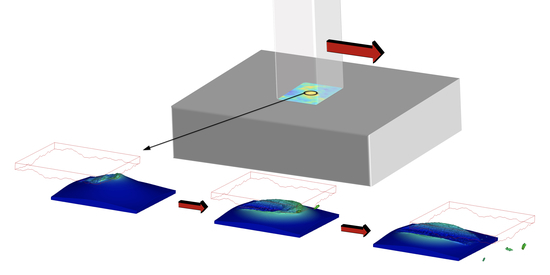
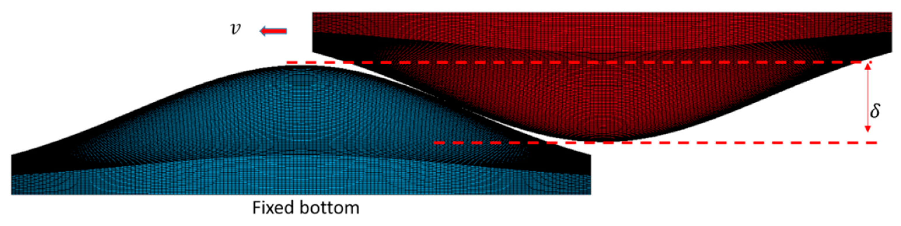
- Set-up the contact problem in the multi-physics Finite Element software LS-DYNA.
- Run the model and analyze the wear results.
4. Results and Discussion
4.1. Model Verification for the Linear Elastic Case
4.2. Case 1—Rigid Body vs. Elasto-Plastic Body
4.3. Case 2—Elasto-Plastic Body vs. Elasto-Plastic Body
4.4. Comparison with BEM
5. Conclusions
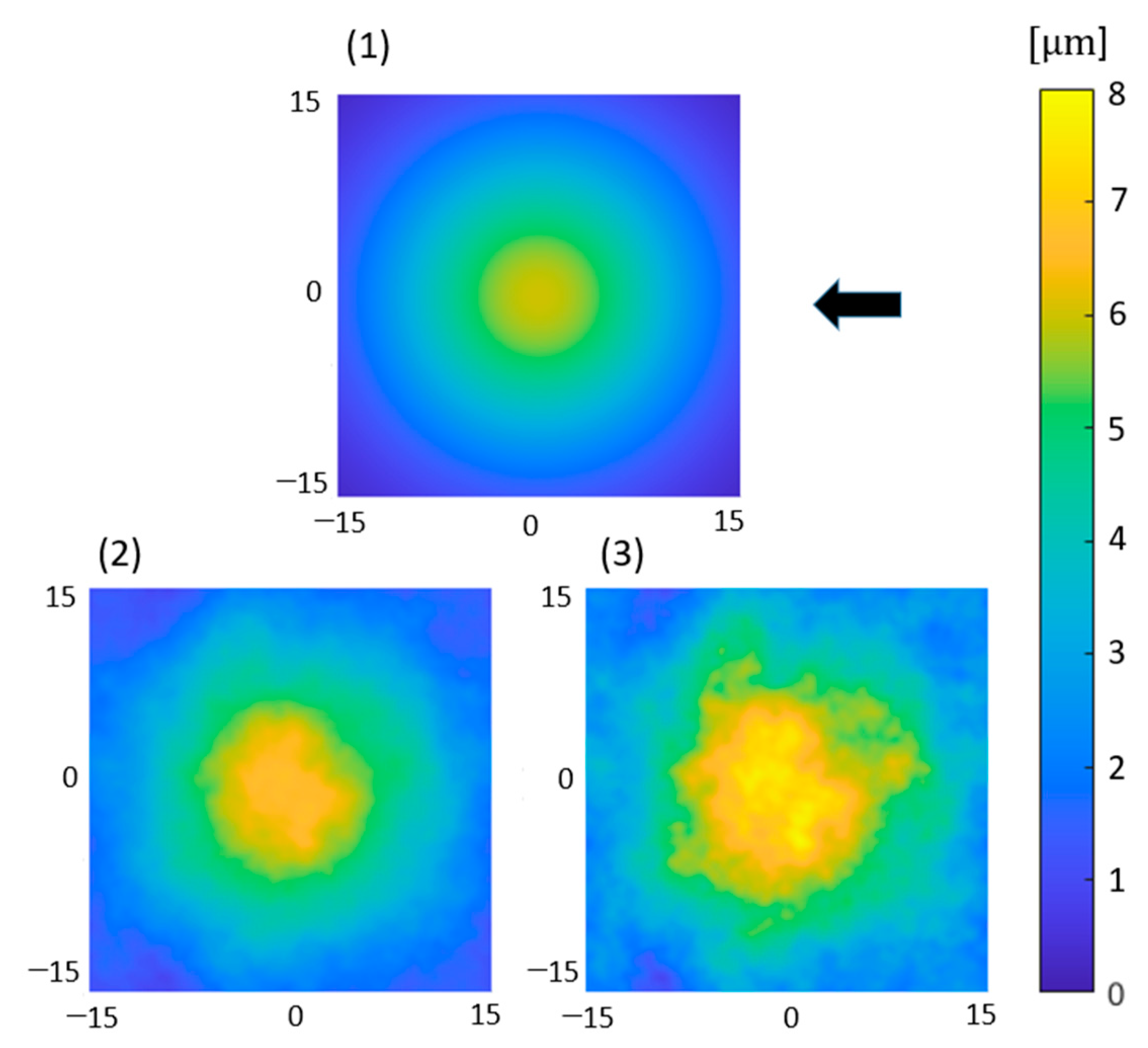
- When a rigid body collides with an elasto-plastically deformable body, the secondary roughness has a significant effect on the wear and temperature development.
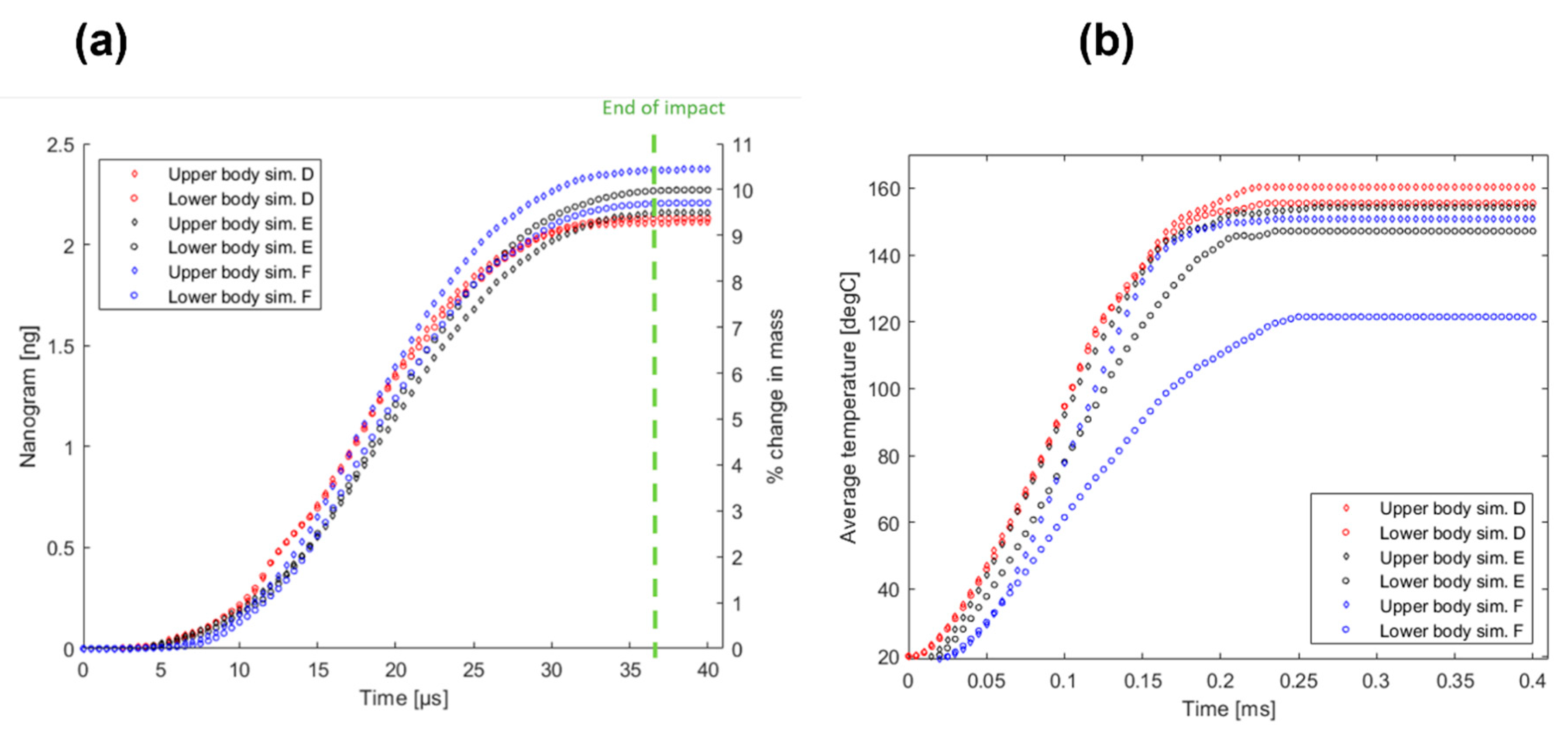
- When two elasto-plastically deformable bodies with the same material properties collide, the effect of the secondary roughness is significantly reduced.
- The wear development is strongly dependent on the triaxiality and Lode parameter, and compressive stresses tend to lead to less wear as compared to shear and tension.
- The flash temperature development is also dependent on the stress state, with compressive stresses leading to higher temperature increases as compared to shear and tension.
Author Contributions
Funding
Conflicts of Interest
References
- Archard, J.F. Wear Theory and mechanisms. In Chapter Wear Control Handbook; ASME: New York, NY, USA, 1980; pp. 39–79. [Google Scholar]
- Zhao, X.; Bhushan, B. Material removal mechanisms of single-crystal silicon on nanoscale and at ultralow loads. Wear 1998, 223, 66–78. [Google Scholar] [CrossRef]
- Kato, K.; Adachi, K. Modern Tribology Handbook, Chapter Wear Mechanisms; CRC Press: Boca Raton, FL, USA, 2000. [Google Scholar]
- Hutchings, I. Wear, Materials, Mechanisms and Practice; Wiley: Hoboken, NJ, USA, 2005. [Google Scholar]
- Hsu, S.; Shen, M. Ceramic wear maps. Wear 1996, 200, 154–175. [Google Scholar] [CrossRef]
- Adachi, K.; Kato, K.; Chen, N. Wear map of ceramics. Wear 1997, 203–204, 291–301. [Google Scholar] [CrossRef]
- Meng, H.; Ludema, K. Wear models and predictive equations: Their form and content. Wear 1995, 443–457 Pt 2, 181–183. [Google Scholar] [CrossRef]
- Furustig, J.; Almqvist, A.; Larsson, R. Numerical simulation of a wear experiment. Wear 2011, 271, 2947–2952. [Google Scholar] [CrossRef]
- Furustig, J.; Larsson, R.; Almqvist, A.; Grahn, M.; Minami, I. Semi-deterministic chemo-mechanical model of boundary lubrication. Faraday Discuss. 2012, 156, 343–360, Discussion 413. [Google Scholar] [CrossRef]
- Jacq, C.; Nelias, D.; Lormand, G.; Girodin, D. Development of a Three-Dimensional Semi-Analytical Elastic-Plastic Contact Code. ASME J. Tribol. 2002, 124, 653–667. [Google Scholar] [CrossRef]
- Sainsot, P.; Jacq, C.; Nelias, D. A Numerical Model for Elastoplastic Rough Contact. Comput. Model. Eng. Sci. 2002, 3, 497–506. [Google Scholar]
- Wang, Z.-J.; Wang, W.-Z.; Hu, Y.-Z.; Wang, H. A Numerical Elastic–Plastic Contact Model for Rough Surfaces. Tribol. Trans. 2010, 53, 224–238. [Google Scholar] [CrossRef]
- Sahlin, F.; Larsson, R.; Almqvist, A.; Lugt, P.; Marklund, P. A mixed lubrication model incorporating measured surface topography: Part 1: Theory of flow factors. Proceedings of the Institution of Mechanical Engineers. Part J J. Eng. Tribol. 2010, 224, 335–351. [Google Scholar] [CrossRef]
- Almqvist, A.; Sahlin, F.; Larsson, R.; Glavatskih, S. On the dry elasto-plastic contact of nominally flat surfaces. Tribol. Int. 2007, 40, 574–579. [Google Scholar] [CrossRef]
- Almqvist, A.; Campañá, C.; Prodanov, N.; Persson, B.N.J. Interfacial separation between elastic solids with randomly rough surfaces: Comparison between theory and numerical techniques. J. Mech. Phys. Solids 2011, 59, 2355–2369. [Google Scholar] [CrossRef]
- Tiwari, A.; Almqvist, A.; Persson, B.N.J. Plastic Deformation of Rough Metallic Surfaces. Tribol. Lett. 2020, 68, 129. [Google Scholar] [CrossRef]
- Pérez Ràfols, F.; Almqvist, A. On the stiffness of surfaces with non-Gaussian height distribution. Sci. Rep. 2021, 11, 1863. [Google Scholar] [CrossRef]
- Pérez Ràfols, F.; Larsson, R.; Riet, E.; Almqvist, A. On the loading and unloading of metal-to-metal seals: A two-scale stochastic approach. Proceedings of the Institution of Mechanical Engineers. Part J J. Eng. Tribol. 2018, 232, 135065011875562. [Google Scholar] [CrossRef]
- Ernens, D.; Pérez Ràfols, F.; Hoecke, D.; Roijmans, R.; Riet, E.; Voorde, J.; Almqvist, A.; Rooij, M.; Roggeband, S.; Haaften, W.; et al. On the Sealability of Metal-to-Metal Seals with Application to Premium Casing and Tubing Connections. SPE Drill. Completion 2019, 34, 382–396. [Google Scholar] [CrossRef]
- Huang, D.; Yan, X.; Larsson, R.; Almqvist, A. Numerical Simulation of Static Seal Contact Mechanics Including Hydrostatic Load at the Contacting Interface. Lubricants 2020, 9, 1. [Google Scholar] [CrossRef]
- Furustig, J.; Almqvist, A.; Bates, C.A.; Ennemark, P.; Larsson, R. A two scale mixed lubrication wearing-in model, applied to hydraulic motors. Tribol. Int. 2015, 90, 248–256. [Google Scholar] [CrossRef][Green Version]
- Fang, L.; Cen, Q.H.; Sun, K.; Liu, W.M.; Zhang, X.F.; Huang, Z.F. FEM Computation of Groove Ridge and Monte Carlo Simulation in Two-Body Abrasive Wear. Wear 2005, 258, 265–274. [Google Scholar] [CrossRef]
- Jain, R.K.; Jain, V.K.; Dixit, P.M. Modeling of Material Removal and Surface Roughness in Abrasive Flow Machining Process. Int. J. Mach. Tools Manuf. 1999, 39, 1903–1923. [Google Scholar] [CrossRef]
- Maekawa, K. Computational Aspects of Tribology in Metal Machining. Proc. Inst. Mech. Eng. Part J J. Eng. Tribol. 1998, 212, 307–318. [Google Scholar]
- Tian, H.; Saka, N. Finite Element Analysis of an Elastic–Plastic Two-Layer Half-Space: Sliding Contact. Wear 1991, 148, 261–285. [Google Scholar] [CrossRef]
- Schermann, T.; Marsolek, J.; Schmidt, C.; Fleischer, J. Aspects of the Simulation of a Cutting Process with ABAQUS/Explicit including the Interaction between the Cutting Process and the Dynamic Behavior of the Machine Tool. In Proceedings of the 9th CIRP International Workshop on Modeling of Machining Operations, Bled, Slovenia, 11–12 May 2006. [Google Scholar]
- Mamalis, A.G.; Vortselas, A.K.; Panagopoulos, C.N. Analytical and Numerical Wear Modeling of Metallic Interfaces: A Statistical Asperity Approach. Tribol. Trans. 2013, 56, 121–129. [Google Scholar] [CrossRef]
- Liu, M.; Proudhon, H. Finite element analysis of frictionless contact between a sinusoidal asperity and a rigid plane: Elastic and initially plastic deformations. Mech. Mater. 2014, 77, 125–141. [Google Scholar] [CrossRef]
- Woldman, M.; van der Heide, E.; Tinga, T.; Masen, M.A. A Finite Element Approach to Modeling Abrasive Wear Modes. Tribol. Trans. 2017, 60, 711–718. [Google Scholar] [CrossRef]
- Johnson, G.R.; Cook, W.H. Fracture Characteristics of Three Metals Subjected to Various Strains, Strain Rates, Temperatures and Pressures. Eng. Fract. Mech. 1985, 21, 31–48. [Google Scholar] [CrossRef]
- Otroshi, M.; Rossel, M.; Meschut, G. Stress state dependent damage modeling of self-pierce riveting process simulation using GISSMO damage model. J. Adv. Join. Processes 2020, 1, 100015. [Google Scholar] [CrossRef]
- Jaeger, J.C. Moving sources of heat and the temperature at sliding surfaces. Proc. R. Soc. New South Wales 1942, 66, 203–224. [Google Scholar]
- Carslaw, H.; Jaeger, J. Conduction of Heat in Solids, 2nd ed.; Clarendon Press: Oxford, UK, 1959. [Google Scholar] [CrossRef]
- Gao, J.; Lee, S.; Ai, X.; Nixon, H. An FFT-Based Transient Flash Temperature Model for General Three-Dimensional Rough Surface Contacts. J. Tribol. Trans. ASME 2000, 122, 555395. [Google Scholar] [CrossRef]
- Liu, S.; Wang, Q. A Three-Dimensional Thermomechanical Model of Contact Between NonConforming Rough Surfaces. J. Tribol. Trans. ASME 2001, 123, 1327585. [Google Scholar] [CrossRef]
- Černe, B.; Duhovnik, J.; Tavčar, J. Semi-analytical flash temperature model for thermoplastic polymer spur gears with consideration of linear thermo-mechanical material characteristics. J. Comput. Des. Eng. 2019, 6, 617–628. [Google Scholar] [CrossRef]
- Yassine, W.; Magnier, V.; Dufrénoy, P.; de saxce, G. Heat partition and surface temperature in sliding contact systems of rough surfaces. Int. J. Heat Mass Transf. 2019, 137, 1167–1182. [Google Scholar] [CrossRef]
- Yassine, W.; Magnier, V.; Dufrénoy, P.; de saxce, G. Multiscale thermomechanical modeling of frictional contact problems considering wear—Application to a pin-on-disc system. Wear 2019, 426–427, 1399–1409. [Google Scholar] [CrossRef]
- Zhang, R.; Guessous, L.; Barber, G. Investigation of the Validity of the Carslaw and Jaeger Thermal Theory under Different Working Conditions. Tribol. Trans. 2011, 55, 1–11. [Google Scholar] [CrossRef]
- Kennedy, F.E. Single Pass Rub Phenomena—Analysis and Experiment. ASME J. Lubr. Tech. 1982, 104, 582–588. [Google Scholar] [CrossRef]
- Effelsberger, J.; Haufe, A.; Feucth, M.; Neukamm, F.; DuBois, P. On parameter identification for the GISSMO damage model. In Proceedings of the 12th International LS-Dyna Users Conference, Detroit, MI, USA, 24 April 2012. [Google Scholar]
- Neukamm, F.; Feucht, M.; Haufe, A. Considering damage history in crashworthiness simulations. In Proceedings of the 7th European LSDyna Conference, Salzburg, SA, USA, 14–15 May 2009. [Google Scholar]
- Lou, H.H. Evaluation of Ductile Fracture Criteria in a General Three-Dimensional Stress State Considering the Stress Triaxiality and the Lode Parameter; Tech. Report; AMSS Press: Wuhan, China, 2012. [Google Scholar]
- Pérez Ràfols, F.; Almqvist, A. Generating randomly rough surfaces with given height probability distribution and power spectrum. Tribol. Int. 2018, 131, 591–604. [Google Scholar] [CrossRef]
- Bai, Y.; Wierzbicki, T. Application of extended Mohr-Coulomb criterion to ductile fracture. Int. J. Fract. 2010, 161, 1. [Google Scholar] [CrossRef]
- LSTC. Ls-Dyna User Manual Volume I. 2018. Available online: https://www.lstc.com/download/manuals (accessed on 7 February 2022).
- Bleck, W.; Frehn, A.; Ohlert, J. Niobium in dual phase and trip steels. In Niobium, Science and Technology; RWTH Aachen University: Aachen, Germany, 2010. [Google Scholar]


| Secondary Roughness | Skewness | Average Roughness Height | RMS Height |
|---|---|---|---|
| i | −0.006 | 0.75 | 0.78 |
| ii | −0.006 | 1.5 | 1.564 |
| Surface # | Secondary Roughness | Skewness | Average Roughness Height | RMS Height |
|---|---|---|---|---|
| 1 | - | 0.55 | 2.6 | 2.68 |
| 2 | i | 0.5 | 3.38 | 3.5 |
| 3 | ii | 0.41 | 4.1 | 4.30 |
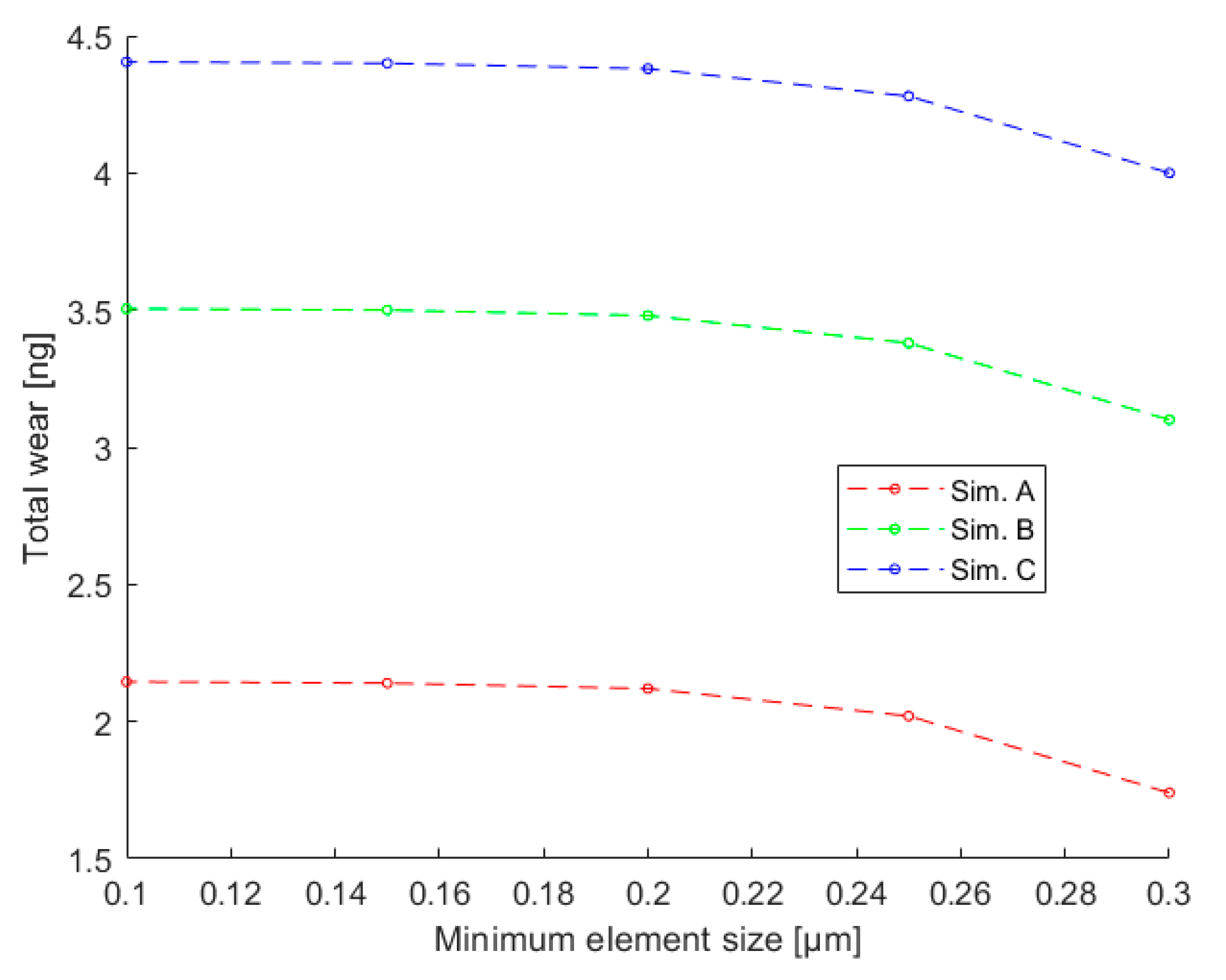
| Simulation # | Upper and Lower Surfaces | Interference [μm] | Speed [m/s] |
|---|---|---|---|
| A | 1 & 1 | 4 | 1 |
| B | 2 & 1 | 4 | 1 |
| C | 3 & 1 | 4 | 1 |
| Simulation # | Upper and Lower Surfaces | Interference [μm] | Speed [m/s] |
|---|---|---|---|
| D | 1 & 1 | 4 | 1 |
| E | 2 & 1 | 4 | 1 |
| F | 3 & 1 | 4 | 1 |
| Elastic Modulus [GPa] | Poisson Ratio | Density [kg/m3] | Specific Heat Capacity [J/(kg K)] | Thermal Conductivity [W/(mK)] | Thermal Expansion Coeff. [1/K] |
|---|---|---|---|---|---|
| 210 | 0.3 | 7850 | 480 | 50 | 0.12×10⁻⁴ |
| Test No. | Test Specimen | |||
|---|---|---|---|---|
| 1 | Dog-bone tension | 0.379 | 1 | 0.751 |
| 2 | Flat specimen with notch | 0.472 | 0.496 | 0.394 |
| 3 | Biaxial tension | 0.667 | −0.921 | 0.950 |
| 4 | Butterfly tension | 0.577 | 0 | 0.460 |
| 5 | Butterfly shear | 0 | 0 | 0.645 |
| 0.265 | |
| [MPa] | 1276 |
| 0.136 | |
| [MPa] | 710 |
| 1.068 |
| Damage Exponent | Critical Damage | Fade Exponent |
|---|---|---|
| 2 | 0.8 | 1 |
Publisher’s Note: MDPI stays neutral with regard to jurisdictional claims in published maps and institutional affiliations. |
© 2022 by the authors. Licensee MDPI, Basel, Switzerland. This article is an open access article distributed under the terms and conditions of the Creative Commons Attribution (CC BY) license (https://creativecommons.org/licenses/by/4.0/).
Share and Cite
Choudhry, J.; Larsson, R.; Almqvist, A. A Stress-State-Dependent Thermo-Mechanical Wear Model for Micro-Scale Contacts. Lubricants 2022, 10, 223. https://doi.org/10.3390/lubricants10090223
Choudhry J, Larsson R, Almqvist A. A Stress-State-Dependent Thermo-Mechanical Wear Model for Micro-Scale Contacts. Lubricants. 2022; 10(9):223. https://doi.org/10.3390/lubricants10090223
Chicago/Turabian StyleChoudhry, Jamal, Roland Larsson, and Andreas Almqvist. 2022. "A Stress-State-Dependent Thermo-Mechanical Wear Model for Micro-Scale Contacts" Lubricants 10, no. 9: 223. https://doi.org/10.3390/lubricants10090223
APA StyleChoudhry, J., Larsson, R., & Almqvist, A. (2022). A Stress-State-Dependent Thermo-Mechanical Wear Model for Micro-Scale Contacts. Lubricants, 10(9), 223. https://doi.org/10.3390/lubricants10090223