Edge Pressures Obtained Using FEM and Half-Space: A Study of Truncated Contact Ellipses


Abstract
:
1. Introduction
2. Methods
2.1. Finite Element Method
2.2. Semi-Analytical Method
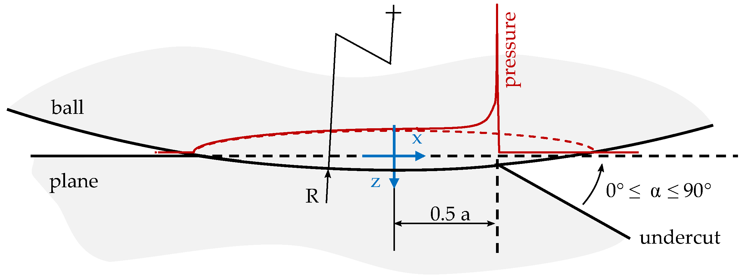
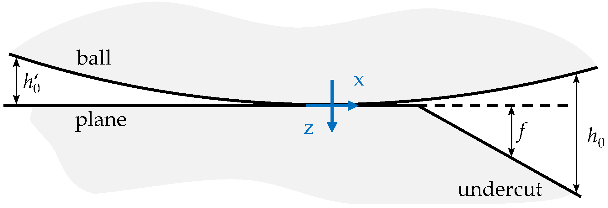
3. Model
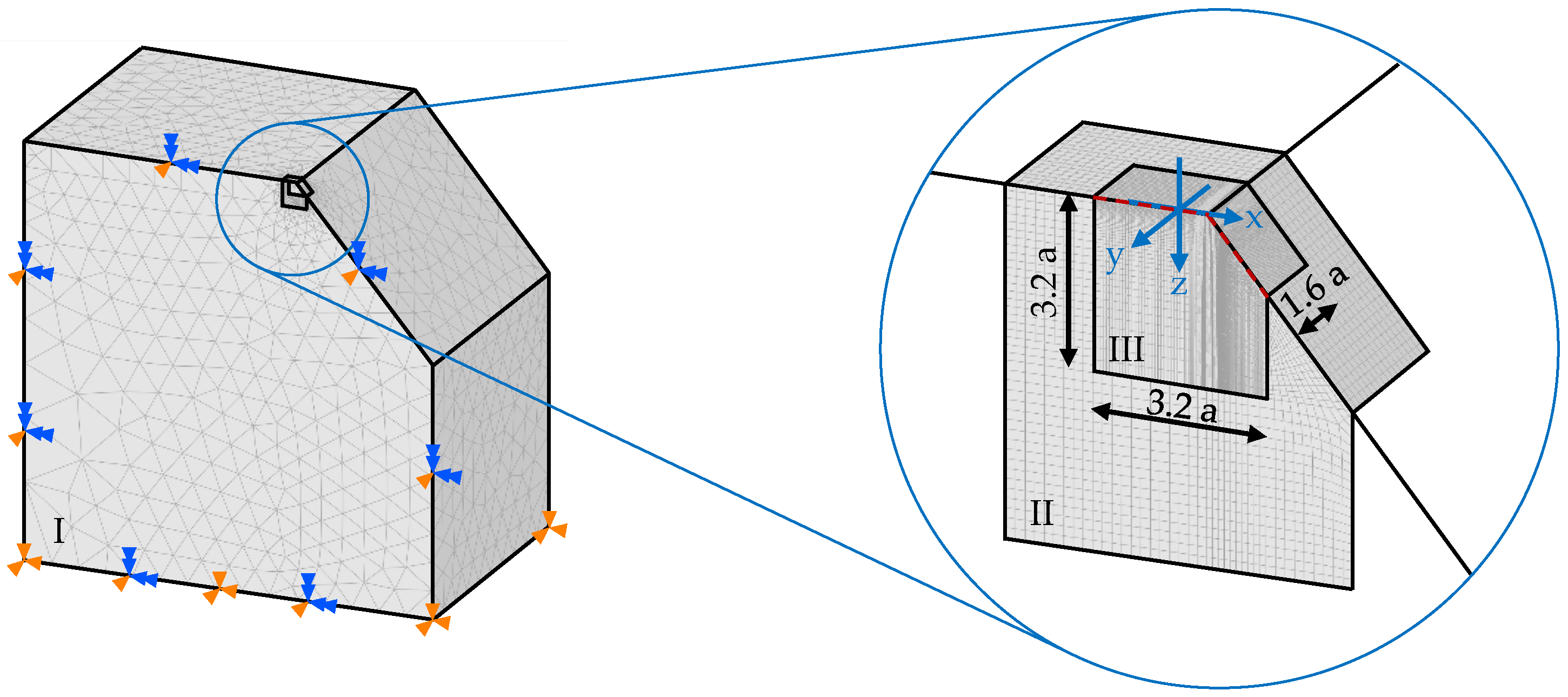
3.1. FEM Model
3.2. SAM Model
4. Results and Discussion
4.1. FEM
4.2. SAM
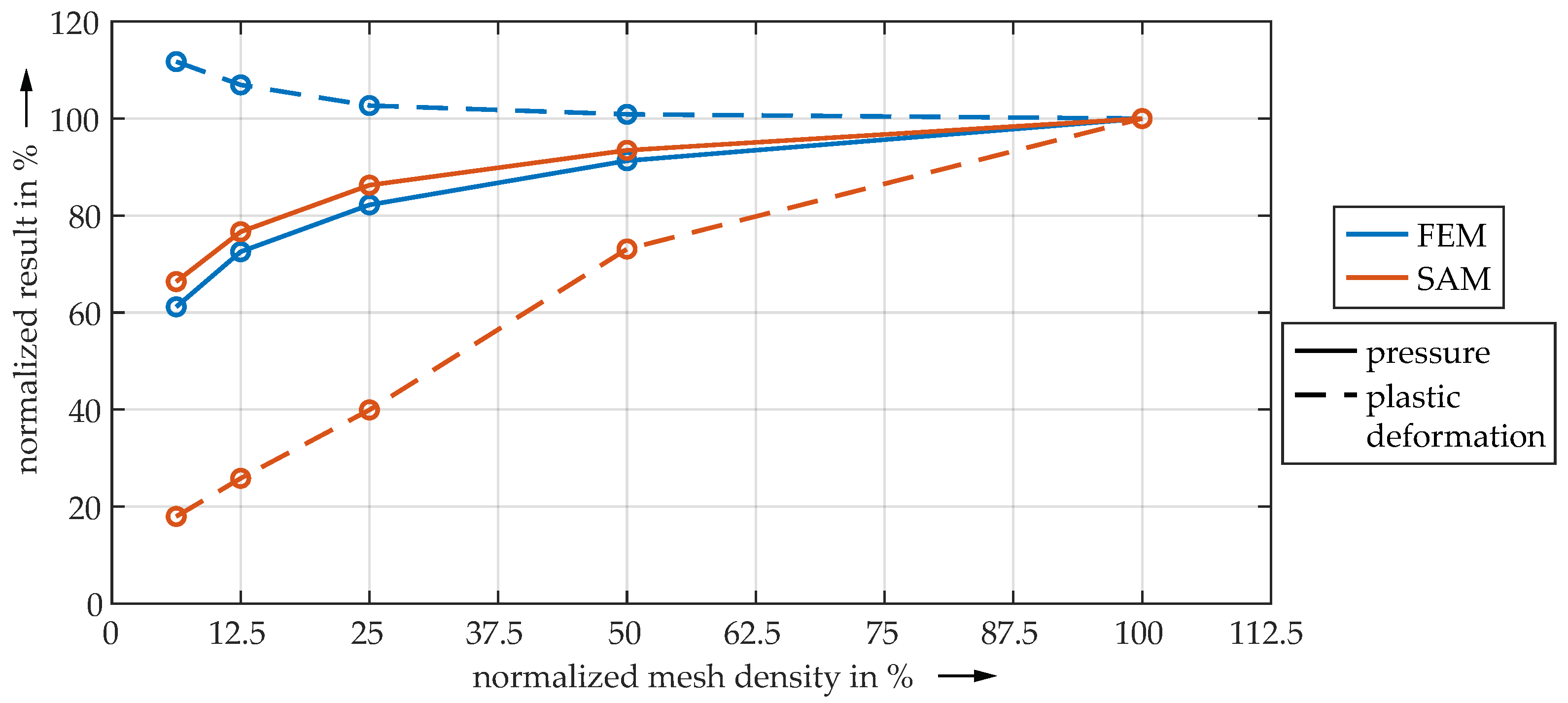
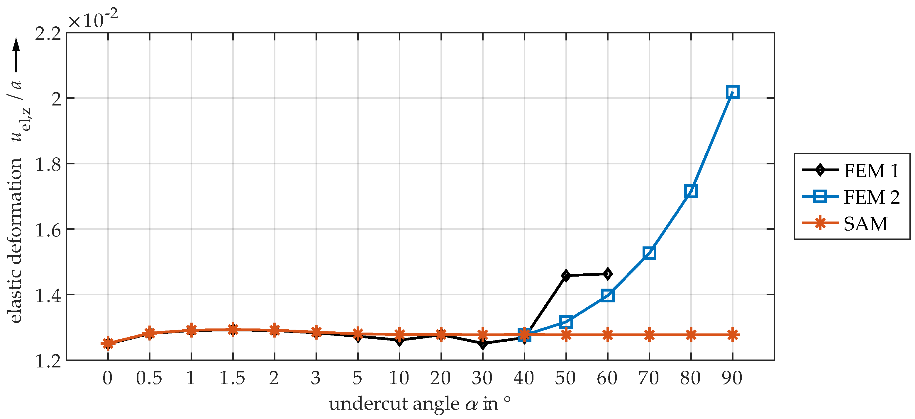
4.3. Comparison of FEM and SAM
5. Conclusions
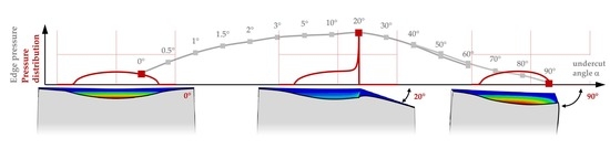
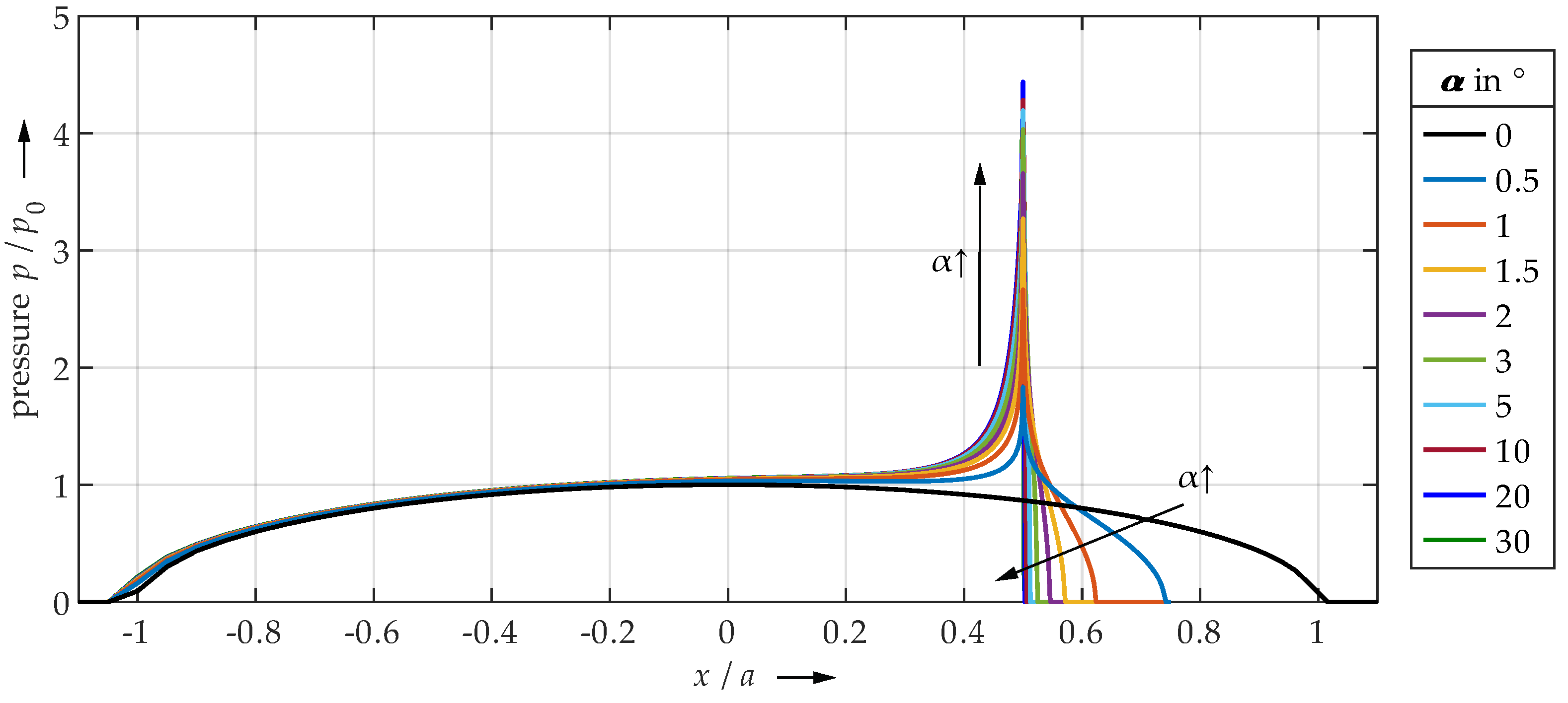
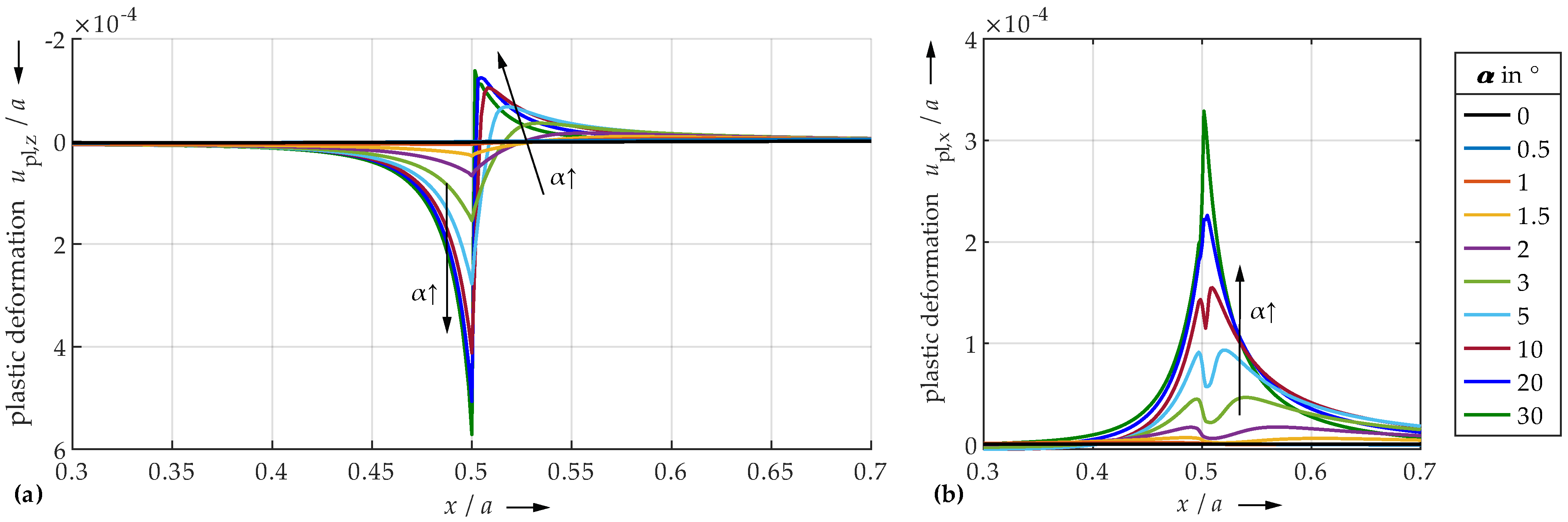
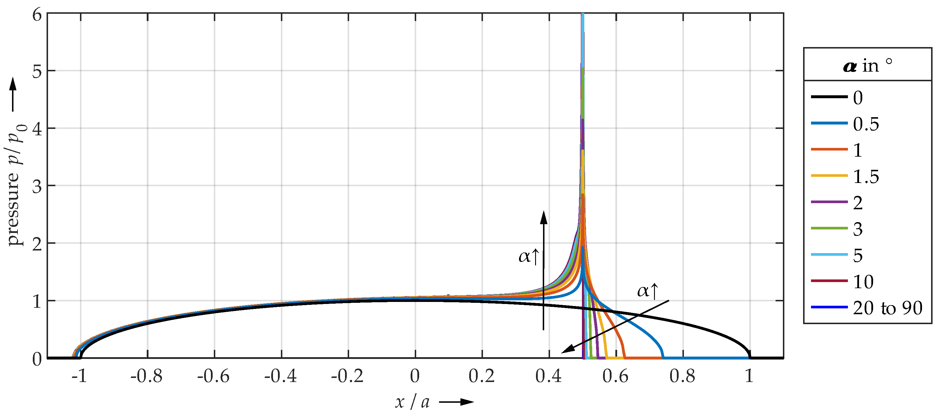
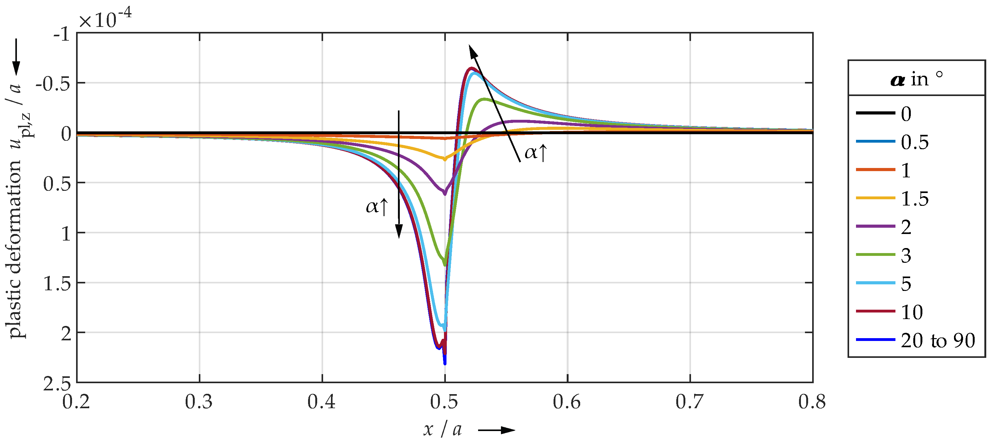
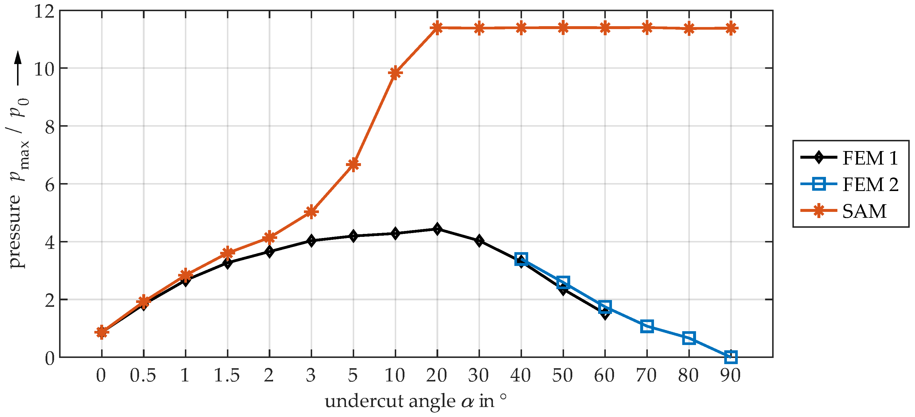
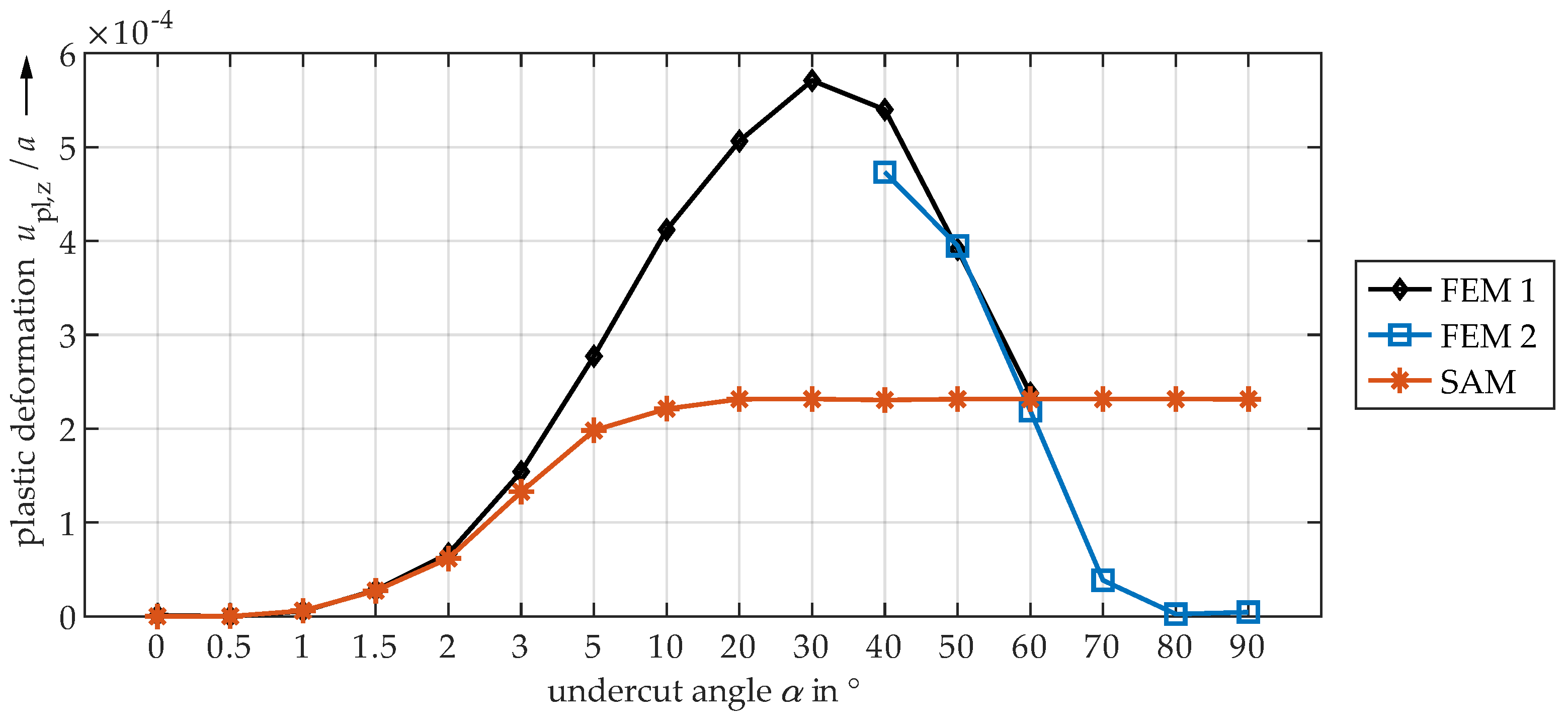
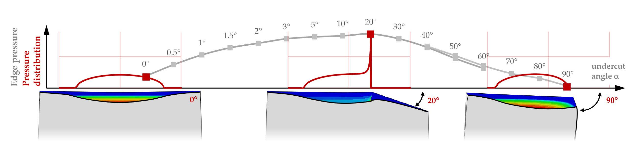
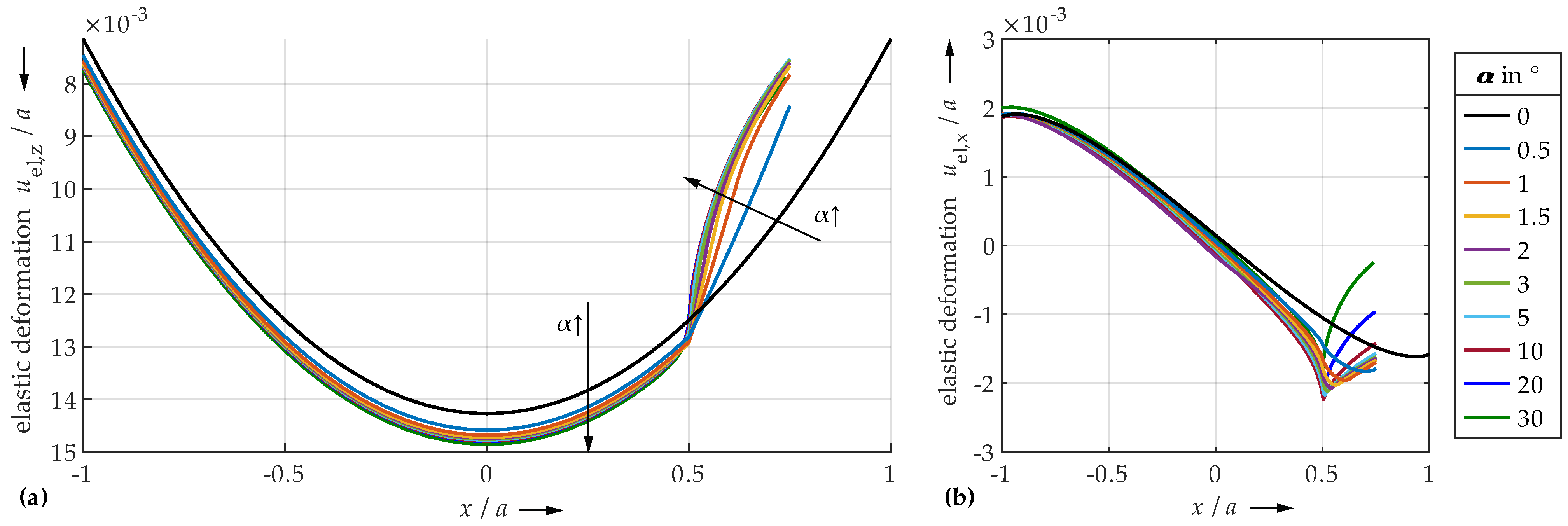
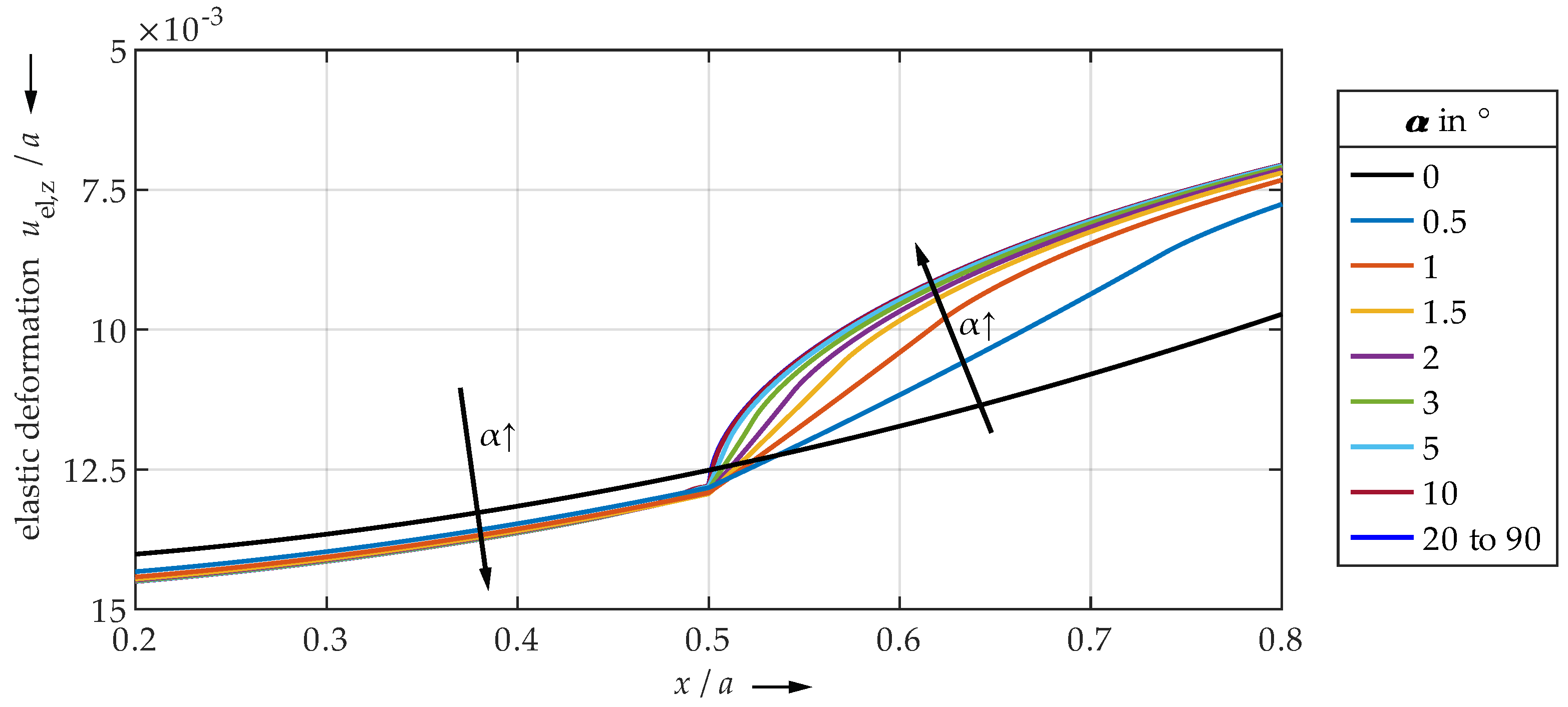
- Very small undercut angles can be considered uncritical. The contact area is slightly limited, but not yet completely delimited by the edge due to deformations. Only moderate pressure peaks and plastic deformations occur.
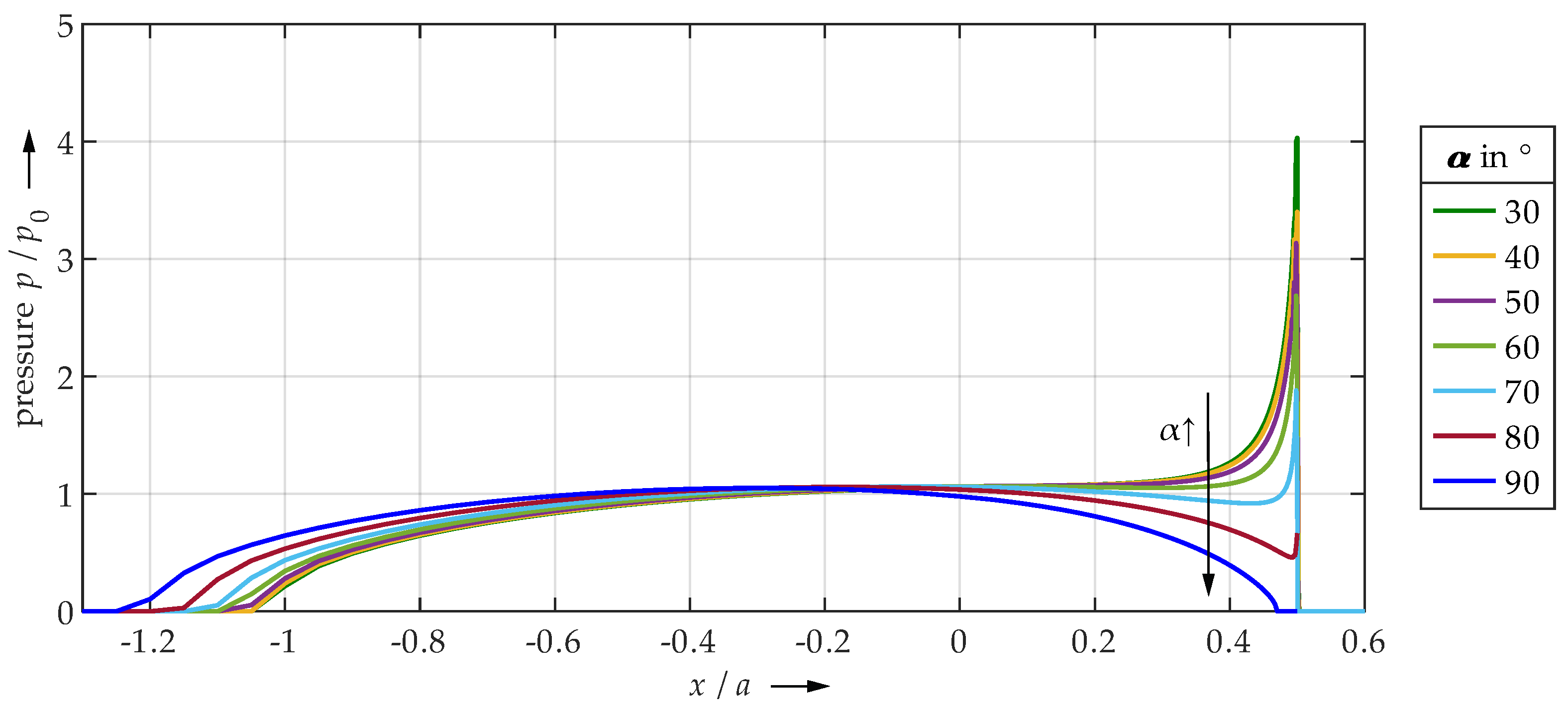
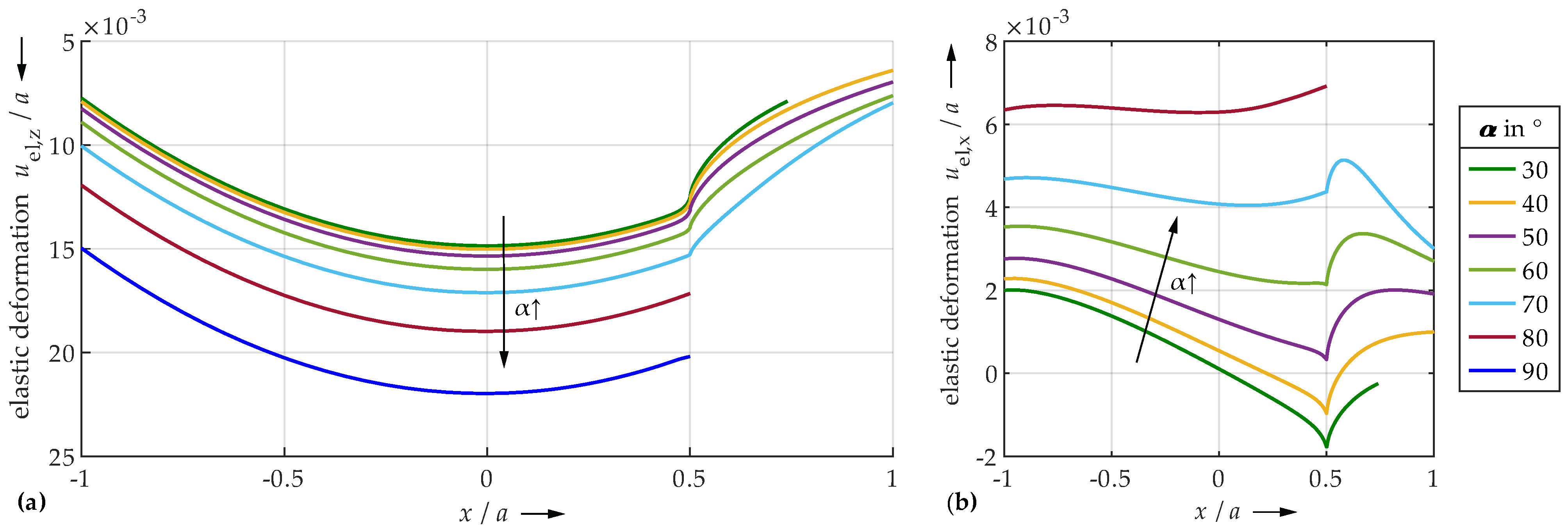
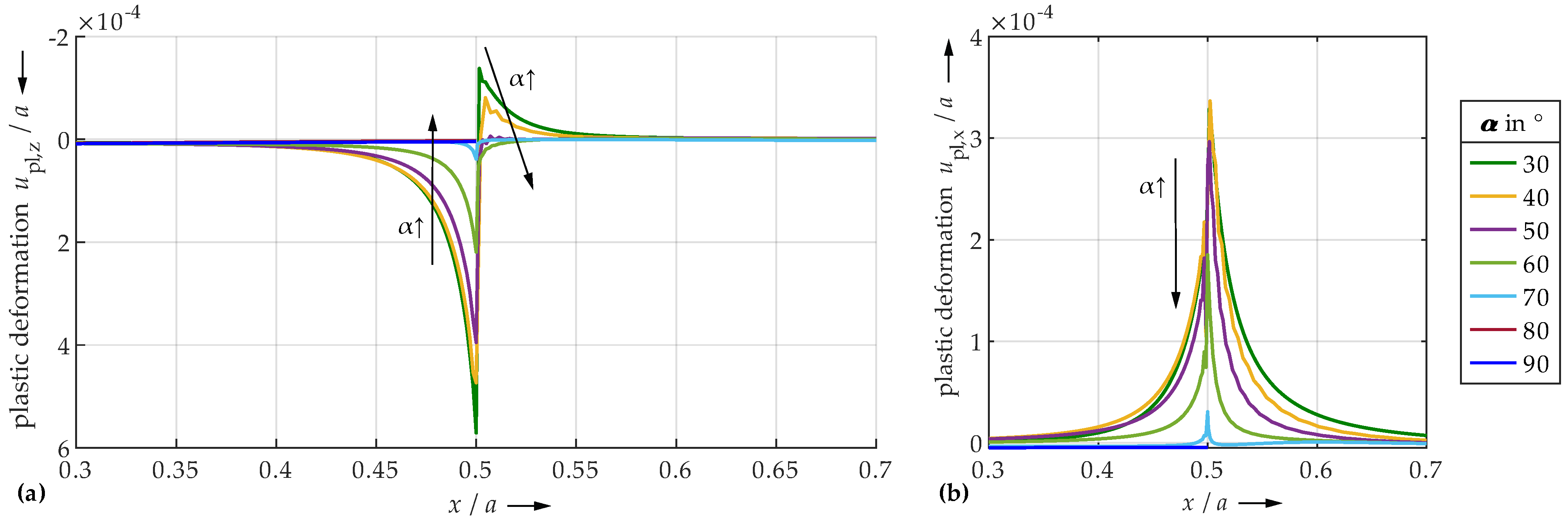
- For very large angles, the contact area is sharply limited by the edge. Due to the steep edge, however, the local structural stiffness of the plane is reduced to such an extent that the entire contact area can deform elastically to a relatively high extent. The edge deflects. Therefore, only minor or no pressure peaks and plastic deformations occur. The contact is significantly characterized by elastic deformation. Thus, also very large angles seem to be uncritical.
- Medium angle ranges result in the highest pressure peaks and plastic deformations, as the contact area is significantly limited by the edge, but the edge still has a high structural stiffness. Elastic deflection of the edge is only marginally possible.
Author Contributions
Funding
Institutional Review Board Statement
Informed Consent Statement
Data Availability Statement
Acknowledgments
Conflicts of Interest
Nomenclature
| a | contact radius given by Hertzian theory |
| B, C, n | Swift isotropic hardening law parameters |
| E | Young’s modulus |
| f | undercut geometry |
| F | applied load |
| h | surface separation |
| initial gap | |
| initial gap without undercut | |
| k, l | indices of the surface grid |
| p | contact pressure |
| maximum contact pressure given by Hertzian theory | |
| maximum contact pressure at the edge | |
| R | radius of the ball |
| u | total surface deformation |
| elastic surface deformation | |
| tangential elastic surface deformation | |
| normal elastic surface deformation | |
| plastic surface deformation | |
| tangential plastic surface deformation | |
| normal plastic surface deformation | |
| x, y, z | space coordinates |
| undercut angle | |
| computational domain | |
| contact area | |
| elastic computational domain (2D) | |
| plastic computational domain (3D) | |
| mesh size | |
| rigid body displacement | |
| effective plastic strain | |
| Poisson’s ratio | |
| yield stress |
References
- Johnson, K.L. Contact Mechanics; Cambridge University Press: Cambridge, Cambridgeshire, UK, 2012. [Google Scholar]
- Hertz, H. Über die Berührung fester elastischer Körper. J. Reine Angew. Math. 1882, 92, 156–171. [Google Scholar] [CrossRef]
- Ghaednia, H.; Wang, X.; Saha, S.; Xu, Y.; Sharma, A.; Jackson, R.L. A Review of Elastic–Plastic Contact Mechanics. Appl. Mech. Rev. 2017, 69, 060804. [Google Scholar] [CrossRef] [Green Version]
- Hardy, C.; Baronet, C.N.; Tordion, G.V. The elastic-plastic indentation of a half-space by a rigid ball. Int. J. Numer. Methods Eng. 1971, 3, 451–462. [Google Scholar] [CrossRef]
- Kogut, L.; Etsion, I. Elastic-Plastic Contact Analysis of a ball and a Rigid Flat. J. Appl. Mech. 2002, 69, 657–662. [Google Scholar] [CrossRef] [Green Version]
- Ghaednia, H.; Mifflin, G.; Lunia, P.; O’Neill, E.O.; Brake, M.R. Strain Hardening from Elastic-Perfectly Plastic to Perfectly Elastic Indentation Single Asperity Contact. Front. Mech. Eng. 2020, 6, 60. [Google Scholar] [CrossRef]
- Jacq, C.; Nélias, D.; Lormand, G.; Girodin, D. Development of a Three-Dimensional Semi-Analytical Elastic-Plastic Contact Code. J. Tribol. 2002, 124, 653–667. [Google Scholar] [CrossRef]
- Nélias, D.; Antaluca, E.; Boucly, V. Rolling of an Elastic Ellipsoid upon an Elastic-Plastic Flat. J. Tribol. 2007, 129, 791–800. [Google Scholar] [CrossRef]
- Boucly, V.; Nélias, D.; Green, I. Modeling of the Rolling and Sliding Contact between Two Asperities. J. Tribol. 2007, 129, 235–245. [Google Scholar] [CrossRef]
- Chen, W.W.; Wang, Q.J.; Wang, F.; Keer, L.M.; Cao, J. Three-Dimensional Repeated elastic-plastic Point Contacts, Rolling, and Sliding. J. Appl. Mech. 2008, 75, 021021. [Google Scholar] [CrossRef]
- Chaise, T.; Nélias, D. Contact Pressure and Residual Strain in 3D elastic-plastic Rolling Contact for a Circular or Elliptical Point Contact. J. Tribol. 2011, 133, 041402. [Google Scholar] [CrossRef]
- Boucly, V.; Nélias, D.; Liu, S.; Wang, Q.J.; Keer, L.M. Contact Analyses for Bodies with Frictional Heating and Plastic Behavior. J. Tribol. 2005, 127, 335–364. [Google Scholar] [CrossRef]
- Nélias, D.; Boucly, V.; Brunet, M. Elastic-Plastic Contact between Rough Surfaces: Proposal for a Wear or Running-In Model. J. Tribol. 2006, 128, 236–244. [Google Scholar] [CrossRef]
- Gallego, L.; Nélias, D.; Deyber, S. A fast and efficient contact algorithm for fretting problems applied to fretting modes I, II and III. Wear 2010, 268, 208–222. [Google Scholar] [CrossRef]
- Hetényi, M. A General Solution for the Elastic Quarter Space. J. Appl. Mech. 1970, 37, 70–76. [Google Scholar] [CrossRef]
- Hanson, M.T.; Keer, L.M. Stress Analysis and Contact Problems for an Elastic Quarter-Plane. Q. J. Mech. Appl. Math. 1989, 42, 364–383. [Google Scholar] [CrossRef]
- Hanson, M.T.; Keer, L.M. A Simplified Analysis for an Elastic Quarter-Space. Q. J. Mech. Appl. Math. 1990, 43, 561–587. [Google Scholar] [CrossRef]
- Zhang, H.; Wang, W.; Zhang, S.; Zhao, Z. Modeling of Finite-Length Line Contact Problem With Consideration of Two Free-End Surfaces. J. Tribol. 2016, 138, 021402. [Google Scholar] [CrossRef]
- Guilbault, R. A Fast Correction for Elastic Quarter-Space Applied to 3D Modeling of Edge Contact Problems. J. Tribol. 2011, 133, 031402. [Google Scholar] [CrossRef]
- Najjari, M.; Guilbault, R. Modeling the edge contact effect of finite contact lines on subsurface stresses. Tribol. Int. 2014, 77, 78–85. [Google Scholar] [CrossRef]
- Polonsky, I.A.; Keer, L.M. A numerical method for solving rough contact problems based on the multi-level multi-summation and conjugate gradient techniques. Wear 1999, 231, 206–219. [Google Scholar] [CrossRef]
- Love, A.E.H. IX. The stress produced in a semi-infinite solid by pressure on part of the boundary. Philos. Trans. R. Soc. 1929, 659–669, 377–420. [Google Scholar] [CrossRef] [Green Version]
- Chiu, Y.P. On the Stress Field Due to Initial Strains in a Cuboid Surrounded by an Infinite Elastic Space. J. Appl. Mech. 1977, 44, 587–590. [Google Scholar] [CrossRef]
- Chiu, Y.P. On the Stress Field and Surface Deformation in a Half-Space with a Cuboidal Zone in Which Initial Strains Are Uniform. J. Appl. Mech. 1977, 45, 302–306. [Google Scholar] [CrossRef]
- Fotiu, P.A.; Nemat-Nasser, S. A universal integration algorithm for rate-dependent elastoplasticity. Comput. Struct. 1996, 59, 1173–1184. [Google Scholar] [CrossRef]
- Liu, S.; Wang, Q.; Liu, G. A versatile method of discrete convolution and FFT (DC-FFT) for contact analyses. Wear 2000, 243, 101–111. [Google Scholar] [CrossRef]
- Swift, H.W. Plastic instability under plane stress. J. Mech. Phys. Solids 1952, 1, 1–18. [Google Scholar] [CrossRef]


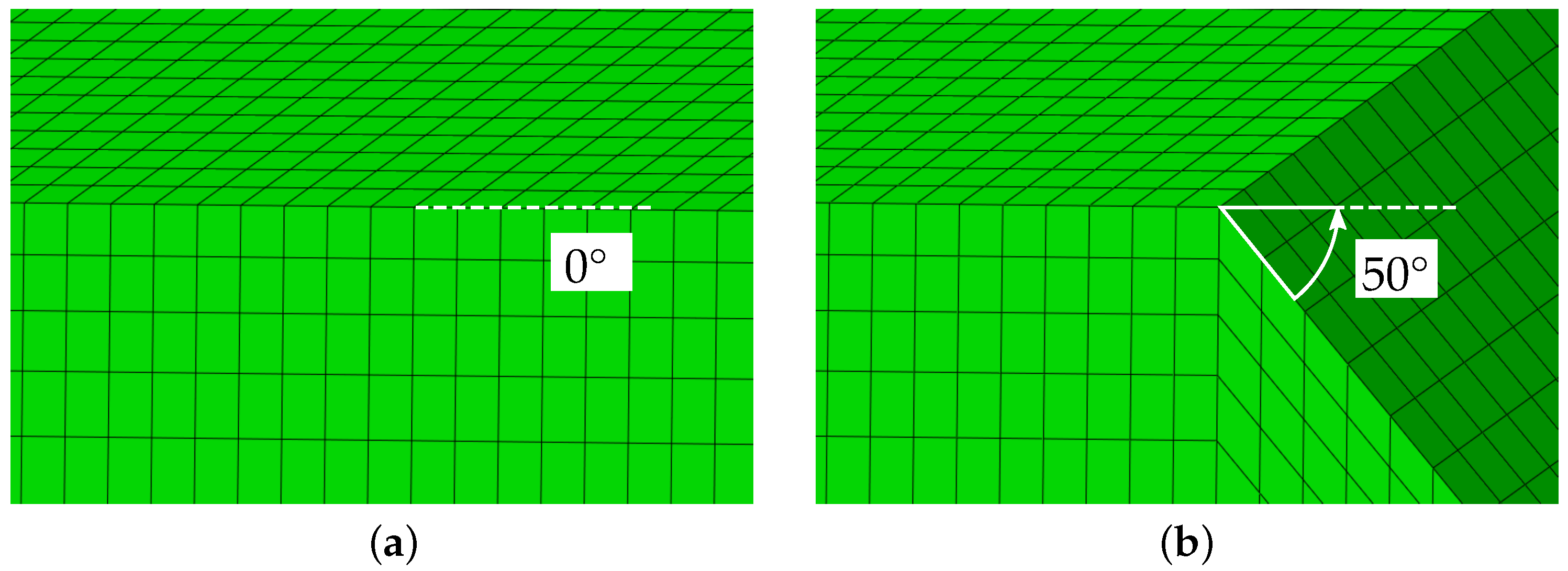
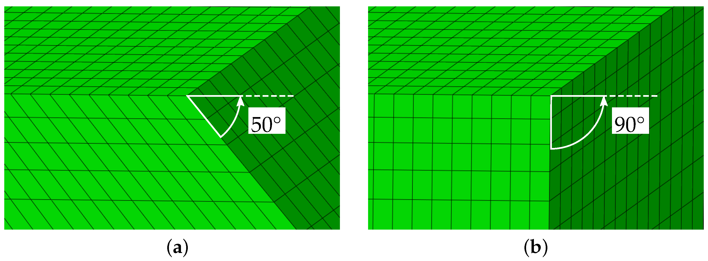
| ↓ Half-Plane | ← Undercut Angle in → | Quarter-Space ↓ | |||||||||||||
|---|---|---|---|---|---|---|---|---|---|---|---|---|---|---|---|
| 0 | 0.5 | 1 | 1.5 | 2 | 3 | 5 | 10 | 20 | 30 | 40 | 50 | 60 | 70 | 80 | 90 |
Publisher’s Note: MDPI stays neutral with regard to jurisdictional claims in published maps and institutional affiliations. |
© 2022 by the authors. Licensee MDPI, Basel, Switzerland. This article is an open access article distributed under the terms and conditions of the Creative Commons Attribution (CC BY) license (https://creativecommons.org/licenses/by/4.0/).
Share and Cite
Juettner, M.; Bartz, M.; Tremmel, S.; Correns, M.; Wartzack, S. Edge Pressures Obtained Using FEM and Half-Space: A Study of Truncated Contact Ellipses. Lubricants 2022, 10, 107. https://doi.org/10.3390/lubricants10060107
Juettner M, Bartz M, Tremmel S, Correns M, Wartzack S. Edge Pressures Obtained Using FEM and Half-Space: A Study of Truncated Contact Ellipses. Lubricants. 2022; 10(6):107. https://doi.org/10.3390/lubricants10060107
Chicago/Turabian StyleJuettner, Michael, Marcel Bartz, Stephan Tremmel, Martin Correns, and Sandro Wartzack. 2022. "Edge Pressures Obtained Using FEM and Half-Space: A Study of Truncated Contact Ellipses" Lubricants 10, no. 6: 107. https://doi.org/10.3390/lubricants10060107
APA StyleJuettner, M., Bartz, M., Tremmel, S., Correns, M., & Wartzack, S. (2022). Edge Pressures Obtained Using FEM and Half-Space: A Study of Truncated Contact Ellipses. Lubricants, 10(6), 107. https://doi.org/10.3390/lubricants10060107