Article

Detectability of Continuous Gravitational Waves from Magnetically Deformed Neutron Stars

by
Jacopo Soldateschi
1,2,3,* and
Niccolò Bucciantini
1,2,3
1
Dipartimento di Fisica e Astronomia, Università degli Studi di Firenze, Via G. Sansone 1, I-50019 Sesto Fiorentino, Italy
2
INAF—Osservatorio Astrofisico di Arcetri, Largo E. Fermi 5, I-50125 Firenze, Italy
3
INFN—Sezione di Firenze, Via G. Sansone 1, I-50019 Sesto Fiorentino, Italy
*
Author to whom correspondence should be addressed.
Galaxies 2021, 9(4), 101; https://doi.org/10.3390/galaxies9040101
Submission received: 8 October 2021 / Revised: 4 November 2021 / Accepted: 7 November 2021 / Published: 10 November 2021

Abstract

:
Neutron stars are known to contain extremely powerful magnetic fields. Their effect is to deform the shape of the star, leading to the potential emission of continuous gravitational waves. The magnetic deformation of neutron stars, however, depends on the geometry and strength of their internal magnetic field as well as on their composition, described by the equation of state. Unfortunately, both the configuration of the magnetic field and the equation of state of neutron stars are unknown, and assessing the detectability of continuous gravitational waves from neutron stars suffers from these uncertainties. Using our recent results relating the magnetic deformation of a neutron star to its mass and radius—based on models with realistic equations of state currently allowed by observational and nuclear physics constraints—and considering the Galactic pulsar population, we assess the detectability of continuous gravitational waves from pulsars in the galaxy by current and future gravitational waves detectors.

1. Introduction

The most dense material objects in the known universe are neutron stars (NSs). While the hypothesis of their existence dates back to the 1930s [1,2], their actual discovery happened more than thirty years later. In 1967, it was pointed out that if NSs were spinning and harboured strong magnetic fields, they would emit electromagnetic waves [3]; during the same year, regular radio pulses from an astrophysical source were discovered [4], and this `pulsar’ was later interpreted to be a NS [5]. Since then, thousands of NSs were discovered. From the perspective of gravitational waves (GWs), two classes of pulsars are of particular interest: millisecond pulsars (MSPs), i.e., pulsars with rotation periods under ∼20 ms, and magnetars, i.e., NSs possessing an extremely strong magnetic field, among the most powerful ever detected [6,7,8,9].
Magnetars were initially discovered as different high energy sources showing either energetic bursting (soft gamma repeaters) or periodic variability (anomalous X-ray pulsars) [10,11,12], and only later shown to be part of the same class of objects. Even though the observed magnetar population is tiny (just over 30 sources [13]) when compared to the known NS population, it is believed that they might actually compose a significant fraction of the young population [14]. While the magnetic field at the surface of pulsars has been inferred to be in the range 10 8 12 G [15,16,17], in magnetars, it is thought to be able to reach 10 15 G [13,18] and even 10 17 18 G in the case of newly-born proto-NSs [19,20,21].
Unfortunately, the geometry and strength of the internal magnetic fields in NSs remains mostly unconstrained: what is known is that neither purely poloidal nor purely toroidal configurations are stable [22,23,24,25,26,27,28], thus favouring a mixed field configurations like the twisted torus [29,30,31]. In any case, magnetic fields of magnetar-like strength can cause potentially observable variations in the phenomenology of NSs, like a modification of their torsional oscillations [32,33], of their cooling properties [34,35] and a deformation in their shape [36,37,38].
This uncertainty adds to the one about the internal properties of matter in NSs, encoded by the equation of state (EoS), which remains largely unknown, even if the observations of NSs with a mass higher than 2 M [39,40] have partly constrained it, ruling out many EoS proposed in the past. Further constraints have come from the NICER telescope [41,42], which has set tighter limits on the possible NS radii, effectively shrinking the allowed region of the mass-radius diagram. In addition, the first observation of GWs emitted by a binary NS merger [43] allowed us to also set limits on the stiffness of the EoS [44].
Today, the internal magnetic field and the EoS of NSs are the two major unknowns in their physics, a problem made more complex by the fact that they are deeply intertwined: strong magnetic fields directly affect the particle composition of NSs, playing a role in particle physics issues like the Delta puzzle [45,46], the hyperon puzzle [47,48], the hadron-quark phase transition [49,50,51,52,53] and the existence of a superconducting phase [54,55,56].
Given that the strong magnetic fields of NSs are able to deform their shape [31,38,57,58,59,60,61], and that a time-varying quadrupolar deformation leads to the emission of continuous GWs (CGWs), it is important to understand the interplay of magnetic fields and the EoS in affecting the magnetic deformation of NSs. In this sense, the existence of relations which are truly independent or weakly dependent on the EoS (quasi-universal relations) relating potentially observable quantities [62,63] may be helpful in disentangling the effects of these two major unknowns.
In this work, we apply our recent results [63,64,65] regarding a quasi-universal relation linking the NS mass, radius, magnetic deformation and surface magnetic field both to the case of the observed pulsar population as contained in the ATNF catalogue [66] and to a generic galactic sample simulated through a population synthesis approach. In particular, we assess the detectability of CGWs through the use of present and future GW detectors, showing that a significant fraction of the MSP population in the galaxy may be observable even with existing detectors when they reach their design sensitivity, while canonical pulsars seem to be beyond the reach of even third generation ones.

2. Materials and Methods

The CGWs strain h 0 emitted by a NS rotating with frequency f rot , at distance d from the detector is
h 0 = 16 π 2 G c 4 Q f rot 2 d ,
where G is Newton’s gravitational constant, c the speed of light, and Q is the quadrupole moment. The quadrupole moment can be written as the product of the relativistic moment of inertia I times the quadrupolar deformation of the NS, e. When the deformation is caused by a purely poloidal magnetic field, the shape of the NS is axisymmetric, and one can approximate with good accuracy
e = | I zz I xx I zz |
where I xx , I zz are the moments of inertia of the NS computed with the Newtonian formula (see Appendix C of [64]), and the z axis is the symmetry axis of the system. It was shown that the Newtonian value of e is a good approximation for the correct GR one [67]. We have found [63,65] that, in GR, for typical magnetic fields of NSs, the magnetic deformation e of a NS is well approximated by the formula
e c s B s 2 ,
where B s is the surface magnetic field at the pole, in units of 10 18 G, and c s is called the `distortion coefficient’. By computing ∼65,000 full GR, multi-dimensional axisymmetric magnetized equilibrium models of NSs with the XNS1 code [31,64,68], adopting a variety of different EoS, we found that c s can be approximated with great accuracy by the following quasi-universal relation:
c s = 2.97 R 10 4.61 M 1.6 2.80 ,
where R 10 = R c / 10 km, M 1.6 = M k / 1.6 M , and R c and M k are the circularisation radius and the Komar mass of the NS, respectively, (see [69,70] for their definition). Incidentally, we remark that it is not the energy of the magnetic field per se that directly gives a gravitational quadrupole, but the oblate/prolate distortion that magnetic pressure and tension produce in the matter distribution inside the NS. This holds for several EoS that satisfy current observational and particle physics constraints, computed according to various techniques and with different particle contents. This approximation also holds for EoS describing strange quark stars (see [71] for an account of the deformation of a NS due to the presence of a quark core), although with a smaller accuracy. On the other hand, it was previously found [62] that the GR moment of inertia I is also well approximated, for a large sample of EoS, by a function of just the mass and radius of the NS. Then, if the rotation frequency, distance, surface magnetic field, mass and radius of a NS are known, one can estimate the strain of the CGWs that it should emit, independently of the EoS. However, the radii of NSs are a notoriously difficult quantity to measure, and for this reason, we chose to consider the two EoS which give the most different radii among the ones we studied (the APR4 [72,73] and the NL3 ω ρ [74,75]), and use them to calculate the radii of the NSs from their mass. With this approach, we expect that the results obtained by considering other EoS should be contained within the limits we find in these two cases.
In the following, we present the results obtained with two different approaches: case study A and case study B. In case A, we generate a population of NSs with the following characteristics: the mass is sampled from a bimodal Gaussian distribution by [76], whose peaks are located at 1.396 M and 1.84 M ; the magnetic field is sampled from a log-normal distribution [77] with mean of 10 12.65 G; the rotation frequency and the distance are taken from the ATNF catalogue [66]. While this distribution is consistent with the observations of canonical pulsars contained in the ATNF catalogue, magnetic fields in MSPs are observed to have much lower values. A possible explanation for this is that the actual magnetic field of MSPs, which distorts their shape, is somehow hidden from observations, either due to an accretion process [78,79] or to ambipolar diffusion [80]. In order to avoid possible selection biases, we chose to re-generate the magnetic field not just for MSPs, but also for canonical pulsars, even if their magnetic fields have been measured. In fact, NSs in the ATNF catalogue tend to have a slightly lower magnetic field than predicted by the aforementioned distribution, possibly due to the fact that pulsars with a stronger magnetic field shut off radio emission more rapidly and have a lower chance of being detected. This sample consists of 3177 NSs, i.e., the present number of NSs contained in the ATNF catalogue minus a few records whose period or distance are missing. Their position in the galaxy can be seen in Figure 1.
Case study B consists of a population of 10 4 NSs, enough to allows us to sample their strain distribution with enough statistical accuracy, with the following characteristics: the mass is computed through three possible Gaussian bimodal mass distributions [the same as in case A [76]; another one peaked at 1.34 M and 1.78 M , with a maximum mass cutoff at 2.9 M [81]; a third one peaked at 1.34 M and 1.47 M [82]; the magnetic field, as before, is sampled from a log-normal distribution [77]; the rotation frequency is computed by fitting the frequency distribution of the ATNF pulsars and then sampling from it; the position is computed by sampling nine different possible galactic distributions [83,84,85,86,87,88,89,90,91]. This corresponds to a total of 28 different populations.
We note here that both the surface magnetic field strength contained in the ATNF catalogue and the one of our selected log-normal distribution refer to the equatorial value, while B s in Equation (3) is that at the pole, which differs by a factor of 2. Moreover, we note that the strain of the plus and cross polarisations h + , × of CGWs emitted at twice the rotation frequency of the NS, contain a factor sin 2 α , where α is the angle between the spin and magnetic axis [92]. This factor, however, is already accounted for in the value of the magnetic field given that, both the ATNF values and the those derived from the log-normal distribution, are given for the case of a magnetic axis orthogonal to the spin axis. This implies that one can obtain h + , × without having to worry about the inclination angle α , because its uncertainty is already factored in into the distribution of magnetic field values.

3. Results

In Figure 2, we can see the predicted strain of CGWs emitted by the NSs in the ATNF catalogue (case study A). Each point represents a given NS in the catalogue, its position on the x - axis being the frequency at which it emits CGWs (twice its rotation frequency). Points are colour-coded according to which EoS has been assumed to calculate the NS radius from its mass, either the APR (red points) or the NL3 ω ρ (blue points). The various curves give the minimum detectable strain of the advanced LIGO (aLIGO) detector at design sensitivity2 (green lines), expected to be achieved during the O4 observing run [93], and of the Einstein Telescope (ET) detector in the D configuration3 (black lines) [94]. The solid lines are the nominal sensitivity curves, while the dot-dashed and dashed lines are the minimum detectable strain in the case of continuous 1 month and 2 years observation time, respectively. For a search over time T, the minimum detectable strain by a ground-based interferometer is [95]
h 0 11.4 S n T ,
where S n is the power spectral density of the detector noise ( S n is the nominal sensitivity curve for the detectors plotted in Figure 2). MSPs, emitting CGWs at a frequency f 50 Hz, and canonical pulsars, form two clearly distinct populations in terms of GWs as can be seen from Figure 2. We see that CGWs emitted by MSPs have a much larger strain, making them potentially observable by both aLIGO and ET with 1 month to 2 years observing time. Concerning the role of the EoS that is used to compute the radii of the NSs, it just has the effect of raising the strain by a factor of 2 to 9 when using the NL3 ω ρ EoS instead of the APR. Canonical pulsars, on the other hand, seem to be mostly invisible to even 3rd generation detectors, even for magnetic fields with the higher strengths.
In order to evaluate the variance of our results, since changes in the mass and magnetic field (which are randomly generated) has the effect of changing the strain for different populations, we repeated the modelling of case A 10 times: for each NS in the ATNF catalogue, with its fixed rotation frequency and distance, we extracted 10 random samples from the mass and magnetic field distributions, effectively generating a population of 63540 NSs (31770 NSs for each of the two EoS). Then, we used Gaussian kernel density estimation (KDE) to evaluate the probability density function of this population. The results are plotted in Figure 3. The red contour plot is the probability density function associated to the our NS population, while the two distribution on the top and right axii are the marginal ones. The green and black lines are the sensitivity curves of the aLIGO and ET detectors, as in Figure 2. The green and black points denote the minima of these curves, and the green and black lines on the axis on the right refer to the values of these minima. The fraction of the NS population that is above those lines is potentially observable with the given instrument and observing time. In particular, using the aLIGO detector with a 1 month (2 years) observation time, ∼ 3 % (∼ 9 % ) of the MSP population could be detected; instead, by using the ET telescope with a 1 month (2 years) observation time, ∼ 16 % (∼ 32 % ) of the MSP population could be detected. In any case, canonical pulsars seem to be out of both detectors’ range. We note that these results are evaluated in the “most optimistic case”, as they are derived under the assumption of a purely poloidal field: if a toroidal component is present, the NSs magnetic deformation is smaller with respect to the case of a pure geometry, resulting in a lower detection rate. So results shown in Figure 2 must be taken as an upper, more optimistic, bound.
Since the pulsars we studied in case A are true astrophysical objects, we estimated the probability of detection of the 5 most promising ones. In order to do so, we chose the 5 NSs, described by the NL3 ω ρ EoS, with the largest median strain computed by considering 100 realisations for their mass and magnetic field. The probability of detection by aLIGO with a 1 month and 2 years observation time, is again computed with a KDE. Results are presented in Table 1.
In order to compute, with sufficient statistical accuracy, the distribution of GW strains for the entire Galactic population of NSs, in the case study B, we generate a population of 10 4 sources. We found that all the combinations of mass and position distributions we have adopted, give similar results regarding the distribution of strains. For this reason, in the following we show and discuss only the results obtained by adopting the same mass distribution as in case A [76] and two position distributions [85,86], denoted in the following as case B1 and case B2, respectively. In the first case, the radial distribution of NSs on the galactic plane is a gamma function peaked at ∼ 5.0 kpc from the galactic centre (model C in the paper [85]), while the distribution above the galactic plane is given by an exponential with a scale height of 330 pc (model S in the same paper). In the second case, the radial distribution is that of NSs at birth [96], given by a gamma function peaked at ∼ 6.2 kpc from the galactic centre, while their height is given by a uniform distribution between 150 pc and 150 pc (model C’ in the paper [86]).
This corresponds to adopting either an evolved population (case B1, more appropriate for old MPS), or a population close to conditions at birth (case B2, more appropriate for young canonical PSRs). The fact that our results show no significant difference in these two cases, is indicative of the fact that any uncertainty in the distribution of NS position in the Galaxy will play a negligible role in assessing their visibility by CGWs. In fact, the biggest difference between cases B1 and B2 lies in the distribution of heights above the Galactic plane, while distances mostly depend only on the radial distribution. The position of the pulsar population generated according to case B1 and case B2 are shown in Figure 4 on the left and right, respectively. In Figure 5, we plot the resulting strain distributions for case study B1 and B2 (top and bottom plots, respectively).
We clearly see that the differences in the resulting strain distribution are minimal, even though the positions of the two populations have a substantially different shape (see Figure 4). In order to estimate the probability density distribution through KDE we increased the number of sources to 10 5 for each EoS, resulting in a total population of 2 × 10 5 NSs. Given that cases B1 and B2 give practically equivalent results regarding h 0 , we only plot the density obtained from case B1 in Figure 6. We see that, using the aLIGO detector with a 1 month (2 years) observation time, ∼ 1 % (∼ 5 % ) of the MSP population could be detected; instead, by using the ET telescope with a 1 month (2 years) observation time, ∼ 10 % (∼ 23 % ) of the MSP population could be detected. As we found in case A, canonical pulsars seem to be out of both detectors’ range.
In the case of a NS endowed with a superconducting core, the extent to which the magnetic field can deform the NS is much more enhanced [58,61]. In this case, we expect NS models to develop a distortion coefficient that is roughly B c 1 / B times higher than cases without a superconducting core, where B c 1 10 15 G is the first critical magnetic field strength and B is the volume averaged magnitude of the magnetic field B [63].
As we show in Figure 7, the fraction of MSPs observable in CGWs is greatly increased in this case: ∼ 18 % (∼ 48 % ) using the aLIGO detector with a 1 month (2 years) observation time and ∼ 69 % (∼ 90 % ) using the ET telescope with a 1 month (2 years) observation time. While the strain of CGWs emitted by canonical pulsars is certainly enhanced by the presence of a superconducting core, next generation telescopes like ET still fall short of the required sensitivity of at least one order of magnitude.

4. Discussion

We have shown that the quasi-universal relation Equation (4) linking the magnetic deformation of a NS to its mass, radius and surface magnetic field can be used to compute the strain of the CGWs they emit in a way that is independent of their EoS. This can be done once the NS mass, radius, surface magnetic field, rotation period and distance are known. Measuring directly the radius is notoriously difficult; however, once an EoS is assumed, there is a one to one relation with the mass, a much easier quantity to estimate, even from a statistical point of view.
For this reason, in order to bound the predictions on CGWs emission, among the many EoS we used to infer the quasi-universal relation for c s , we have chosen the two that give the most different radii, for the same NS mass. In this way, we are confident that our results regarding the possible GW detectability of the Galactic NS population should remain valid also for other EoS. As we discussed, the strain computed by adopting these two EoS can differ by up to an order of magnitude, and this can be taken as an estimate of the uncertainty due to our ignorance of the NS internal composition. In order to evaluate how other properties of Galactic NSs, like their magnetic field and period distribution, play a role, we adopted two different approaches. In case A, we used the values for the rotation period and distance of the known pulsars in the galaxy, given by the ATNF catalogue, and we assigned to them a mass and surface magnetic field from the expected distributions. In the other case B, we synthesised the whole galactic NS population by assigning to each one of them all the necessary quantities (magnetic field, mass, rotation period, distance) from the expected distributions, allowing us to compute the strain of potentially undetected sources.
In the last case, we also sampled a variety of distributions both for their mass and for their location in the galaxy, finding very similar results in all cases, which suggest that the uncertainty in these two quantities is not dominant over the one for the strength of the magnetic field. In order to evaluate the detection probability, for each one of the EoS we selected, we randomly generated a large population, and computed the density distribution of h 0 using a KDE approach. This allows us to estimate the fraction of NSs in the galaxy whose CGWs are within the range of ground-based future GW detectors. In particular, we considered the cases of the aLIGO and the ET detectors, either for continuous 1 month or 2 years observation time. In case A, considering a 2 years observing time, (see Figure 3) we found that up to ∼ 9 % and ∼ 32 % of the total MSPs population lies within the reach of aLIGO and ET, respectively. This amounts to a number of ∼270 and ∼960 detectable pulsars if one considers the expected number ∼ 3 × 10 3 of MSPs within 5 kpc of the Sun [97]. We note that those are the NSs that, due to their beaming geometry, are expected to be detectable as pulsating radios sources. In general, a large fraction of the total pulsar population would not be detectable in radio, due to their beaming geometry, but they may be observable through their CGWs emission. Lower total fractions are obtained in case B1 (see Figure 6): up to ∼ 5 % and ∼ 23 % of the total MSP population with aLIGO and ET, respectively, corresponding to ∼2000 and ∼9200 NSs considering the ∼ 4 × 10 4 MSPs expected to be present in the Galaxy [97]. This is simply a selection bias because, as we see in Figure 1—top plot—the NS population of the ATNF catalogue is roughly centred on the position of the Solar System (Galactocentric coordinates ( x , y , z ) = ( 8.122 , 0 , 0.021 ) kpc), and much closer to us than the average Galactic population, thus making it potentially easier to detect.
We also considered the possibility of NSs to be endowed with a superconducting core. In this case, the effective internal magnetic field that deforms the star is much stronger that the magnetic field outside the NS (the one responsible for the spin-down), and this implies a potentially much stronger emission of CGWs by the same sources. In fact, under this assumption, the fraction of detectable MSPs can reach values up to ∼ 48 % and even ∼ 90 % in the case of a 2 year observation with aLIGO and ET, respectively, corresponding to ∼19,200 and ∼36,000 NSs. Even with just one month of observing time, ∼ 18 % and ∼ 69 % of the MSPs in the Galaxy lie within the reach of aLIGO and ET, amounting to ∼7200 and ∼27,600 objects, respectively. However, even in the presence of superconductivity, CGWs emitted by canonical pulsars seem to be far too weak even for 3rd generation ground-based GW detectors, due to their slow rotation period. On the other hand, given that such a large fraction of MSPs could be detectable by aLIGO and ET in the case of superconductivity, the absence of any CGWs detection could itself be an indication of the lack of a superconducting core, effectively constraining the possibility of its existence.
We would like to remark that all of our models are fully multi-dimensional and computed in full GR, by solving simultaneously the Einstein, Euler and Maxwell equations. It is only in the calculation of the distortion e that we have used an integral formula derived in the Newtonian limit (still performed over the GR solution for the matter-energy distribution). This is because for non-liner GR codes, like the one we have used, this approach is numerically more robust than the correct GR one based on the asymptotic vanishing metric terms which, for small deformations, are subject to large numerical noise. Moreover, this approach has been shown in the past to give results in good accordance with the exact GR approach.
We wish to recall here that our results have been derived under the assumption that the magnetic field inside NSs was a purely poloidal. While this is clearly a simplifying assumption, it provides an upper bound on the deformability, and as such can be used to infer information on the geometry of the internal magnetic field. Indeed, a lack of detection would be a strong indication that a toroidal magnetic field component is present in the interior, which counteracts the effect of the poloidal term, and could be used to set limits on the relative strength of the two.
As a final cautionary remark, let us recall that the detectability of CGWs from a NS is not just a function of their strain h 0 , but also of its orientation with respect to the detectors and of the inclination between the magnetic and the rotation axis. GW detectors have a particular antenna pattern which renders them more or less sensitive to waves coming from certain angular positions in the sky. While we believe our work can give a comprehensive overview of what to expect in terms of CGWs emission by pulsars in the Galaxy, a more in depth analysis would have to also take into account the expected distribution of the relative inclination between the magnetic and spin axis, as well as to consider the time-varying angular position of the NS with respect to the ground-based detectors on Earth.

Author Contributions

Conceptualization, J.S. and N.B.; data curation, J.S. and N.B.; formal analysis, J.S. and N.B.; investigation, J.S. and N.B.; writing—original draft, J.S.; writing—review and editing, N.B. All authors have read and agreed to the published version of the manuscript.

Funding

The authors acknowledge financial support from the Accordo Attuativo ASI-INAF n. 2017-14-H.0 `On the escape of cosmic rays and their impact on the background plasma’, the PRIN-INAF 2019 `Short gammaray burst jets from binary neutron star mergers’ and from the INFN Teongrav collaboration.

Institutional Review Board Statement

Not applicable.

Informed Consent Statement

Not applicable.

Data Availability Statement

The data presented in this study are available on request from the corresponding author.

Conflicts of Interest

The authors declare no conflict of interest.

Notes

1
The XNS code solves simultaneously and self-consistently the Einstein equations for the metric, the GRMHD-Euler Equation for the plasma, and the GR-Maxwell Equations for the magnetic field distribution, using the XCFC formalism.
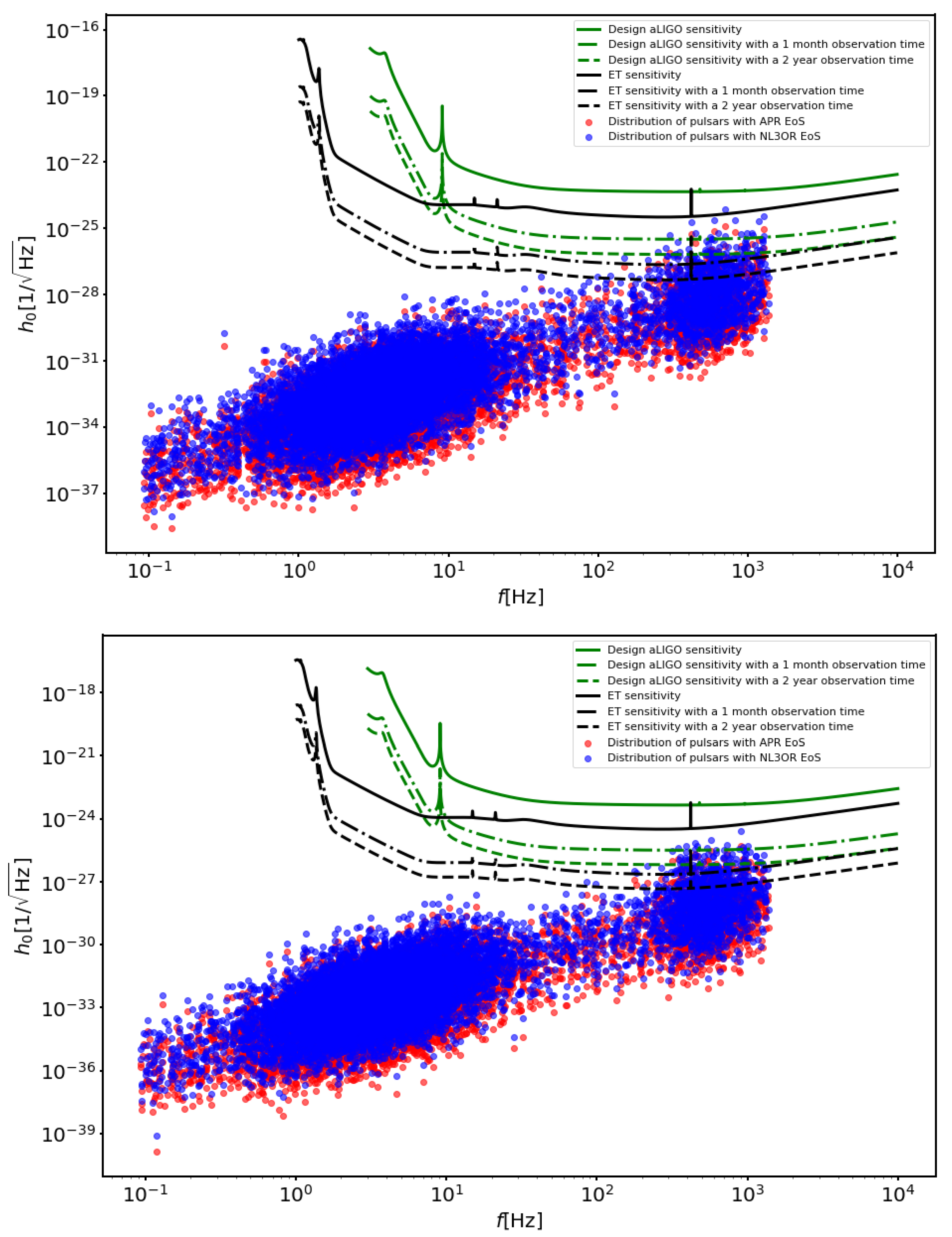
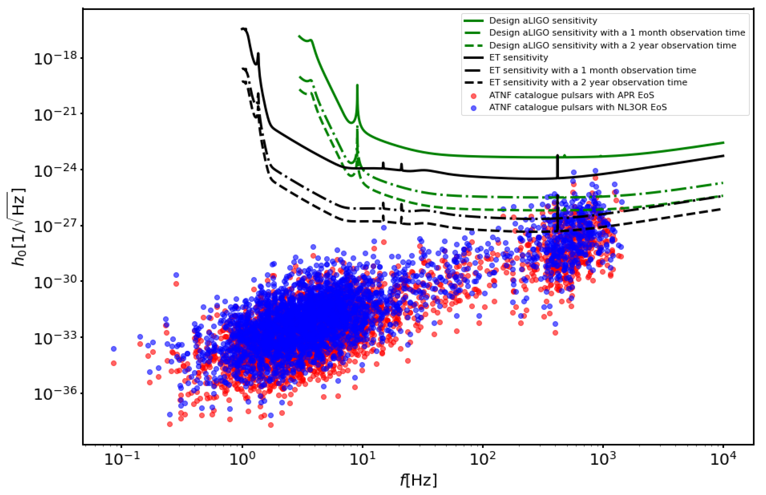
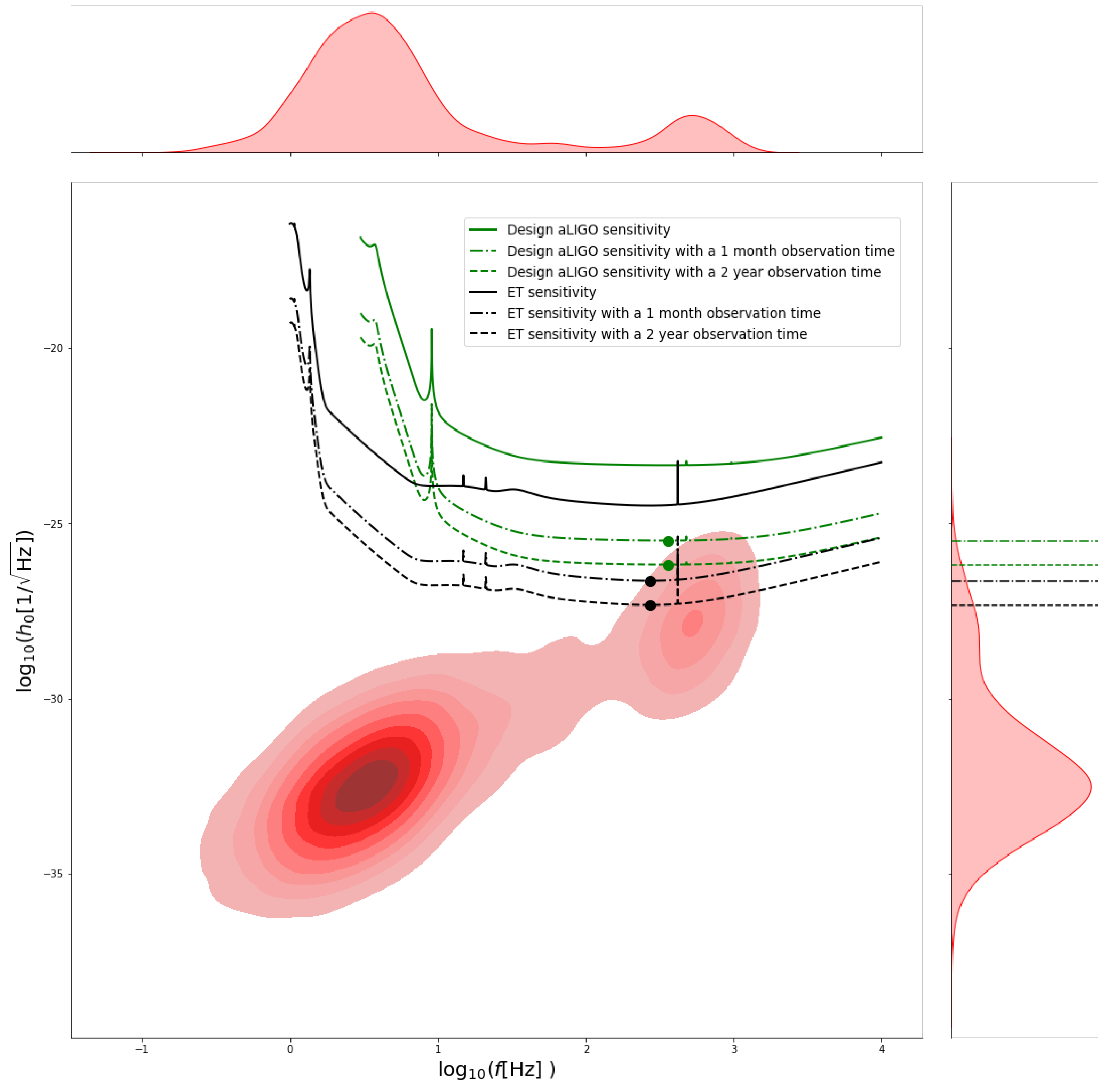
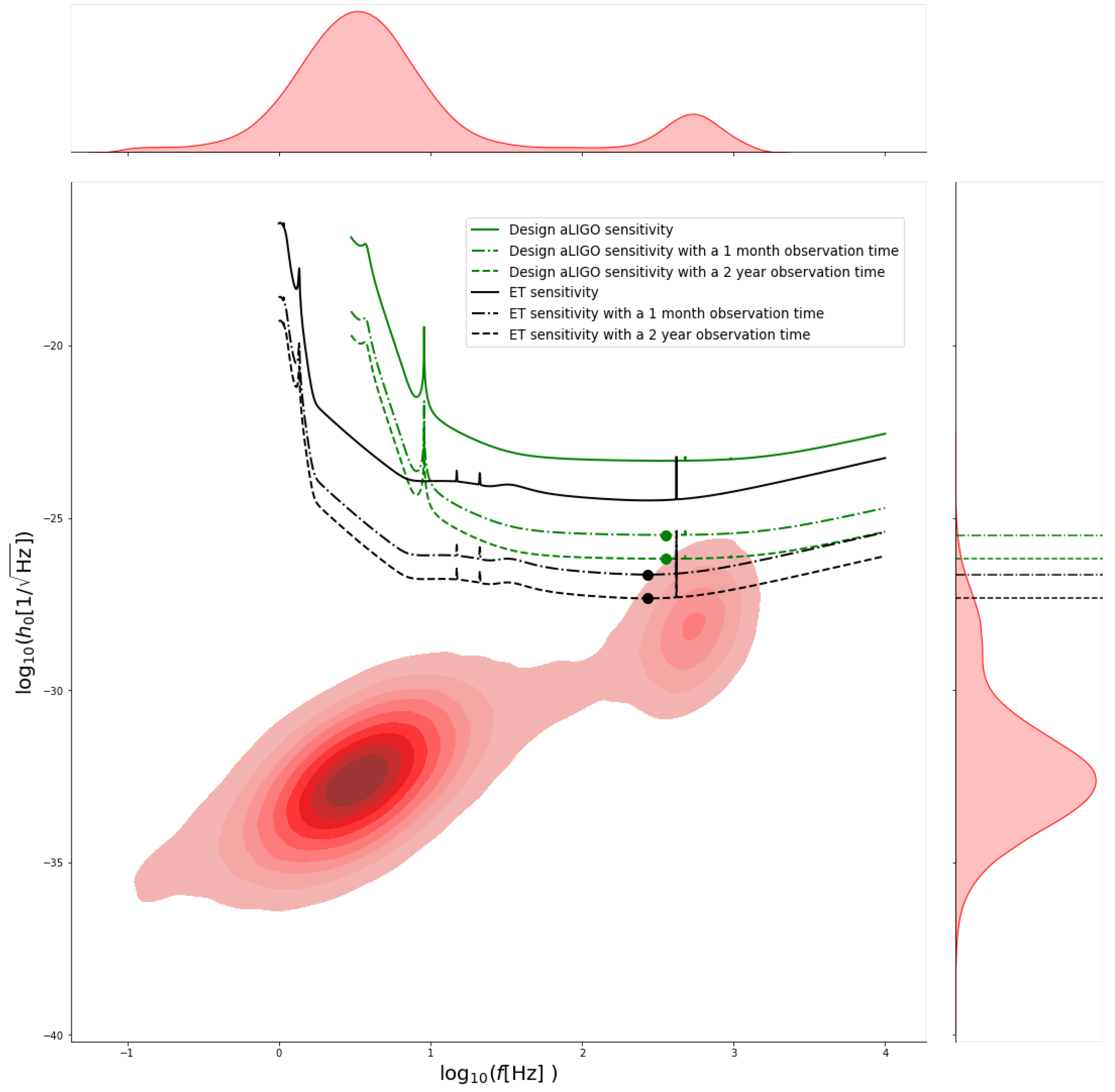
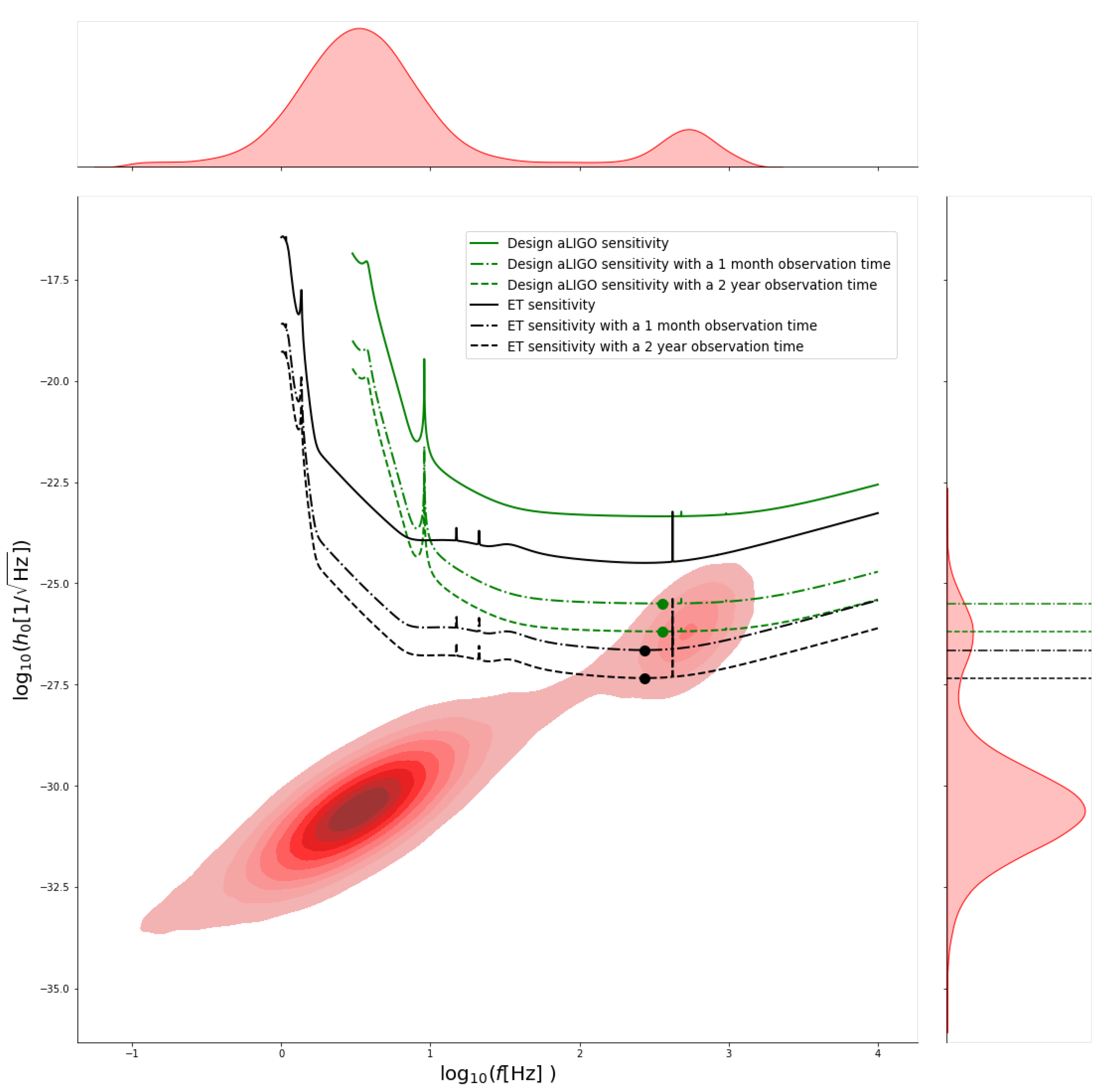
2
The aLIGO design densitivity curves can be found at https://dcc.ligo.org/LIGO-T1800044/public, (accessed on 14 September 2021).
3
The ET sensitivity curves can be found at http://www.et-gw.eu/index.php/etsensitivities, (accessed on 14 September 2021).

References

  1. Landau, L.D. To the theory of energy transmission in collissions. II. Phys. Zs. Sowjet 1932, 2, 46. [Google Scholar]
  2. Baade, W.; Zwicky, F. On Super-novae. Proc. Natl. Acad. Sci. USA 1934, 20, 254–259. [Google Scholar] [CrossRef] [PubMed] [Green Version]
  3. Pacini, F. Energy Emission from a Neutron Star. Nature 1967, 216, 567–568. [Google Scholar] [CrossRef]
  4. Hewish, A.; Bell, S.J.; Pilkington, J.D.H.; Scott, P.F.; Collins, R.A. Observation of a Rapidly Pulsating Radio Source. Nature 1968, 217, 709–713. [Google Scholar] [CrossRef]
  5. Gold, T. Rotating Neutron Stars as the Origin of the Pulsating Radio Sources. Nature 1968, 218, 731–732. [Google Scholar] [CrossRef]
  6. Duncan, R.C.; Thompson, C. Formation of Very Strongly Magnetized Neutron Stars: Implications for Gamma-Ray Bursts. ApJ 1992, 392, L9. [Google Scholar] [CrossRef]
  7. Thompson, C.; Duncan, R.C. Neutron Star Dynamos and the Origins of Pulsar Magnetism. ApJ 1993, 408, 194. [Google Scholar] [CrossRef]
  8. Thompson, C.; Duncan, R.C. The soft gamma repeaters as very strongly magnetized neutron stars—I. Radiative mechanism for outbursts. MNRAS 1995, 275, 255–300. [Google Scholar] [CrossRef]
  9. Thompson, C.; Duncan, R.C. The Soft Gamma Repeaters as Very Strongly Magnetized Neutron Stars. II. Quiescent Neutrino, X-Ray, and Alfven Wave Emission. ApJ 1996, 473, 322. [Google Scholar] [CrossRef]
  10. Kouveliotou, C.; Dieters, S.; Strohmayer, T.; van Paradijs, J.; Fishman, G.J.; Meegan, C.A.; Hurley, K.; Kommers, J.; Smith, I.; Frail, D.; et al. An X-ray pulsar with a superstrong magnetic field in the soft γ-ray repeater SGR1806 - 20. Nature 1998, 393, 235–237. [Google Scholar] [CrossRef]
  11. Gavriil, F.P.; Kaspi, V.M.; Woods, P.M. Magnetar-like X-ray bursts from an anomalous X-ray pulsar. Nature 2002, 419, 142–144. [Google Scholar] [CrossRef] [PubMed]
  12. Mereghetti, S.; Pons, J.; Melatos, A. Magnetars: Properties, Origin and Evolution. Space Sci. Rev. 2015, 191, 315–338. [Google Scholar] [CrossRef] [Green Version]
  13. Olausen, S.A.; Kaspi, V.M. The McGill Magnetar Catalog. ApJS 2014, 212, 6. [Google Scholar] [CrossRef] [Green Version]
  14. Kaspi, V.M.; Beloborodov, A.M. Magnetars. ARA&A 2017, 55, 261–301. [Google Scholar] [CrossRef] [Green Version]
  15. Asseo, E.; Khechinashvili, D. The role of multipolar magnetic fields in pulsar magnetospheres. MNRAS 2002, 334, 743–759. [Google Scholar] [CrossRef] [Green Version]
  16. Spruit, H.C. The source of magnetic fields in (neutron-) stars. In Cosmic Magnetic Fields: From Planets, to Stars and Galaxies; Strassmeier, K.G., Kosovichev, A.G., Beckman, J.E., Eds.; Cambridge University Press: Cambridge, UK, 2009; Volume 259, pp. 61–74. [Google Scholar] [CrossRef] [Green Version]
  17. Ferrario, L.; Melatos, A.; Zrake, J. Magnetic Field Generation in Stars. Space Sci. Rev. 2015, 191, 77. [Google Scholar] [CrossRef] [Green Version]
  18. Popov, S.B. Origins of magnetars in binary systems. Astron. Astrophys. Trans. 2016, 29, 183–192. [Google Scholar]
  19. Del Zanna, L.; Bucciantini, N. Covariant and 3 + 1 equations for dynamo-chiral general relativistic magnetohydrodynamics. MNRAS 2018, 479, 657–666. [Google Scholar] [CrossRef]
  20. Ciolfi, R.; Kastaun, W.; Kalinani, J.V.; Giacomazzo, B. First 100 ms of a long-lived magnetized neutron star formed in a binary neutron star merger. Phys. Rev. D 2019, 100, 023005. [Google Scholar] [CrossRef] [Green Version]
  21. Franceschetti, K.; Del Zanna, L. General Relativistic Mean-Field Dynamo Model for Proto-Neutron Stars. Universe 2020, 6, 83. [Google Scholar] [CrossRef]
  22. Prendergast, K.H. The Equilibrium of a Self-Gravitating Incompressible Fluid Sphere with a Magnetic Field. I. ApJ 1956, 123, 498. [Google Scholar] [CrossRef]
  23. Chandrasekhar, S.; Prendergast, K.H. THE EQUILIBRIUM OF MAGNETIC STARS. Proc. Natl. Acad. Sci. USA 1956, 42, 5–9. [Google Scholar] [CrossRef] [Green Version]
  24. Chandrasekhar, S.; Kendall, P.C. On Force-Free Magnetic Fields. ApJ 1957, 126, 457. [Google Scholar] [CrossRef]
  25. Tayler, R.J. The adiabatic stability of stars containing magnetic fields-I.Toroidal fields. MNRAS 1973, 161, 365. [Google Scholar] [CrossRef]
  26. Markey, P.; Tayler, R.J. The adiabatic stability of stars containing magnetic fields. II. Poloidal fields. MNRAS 1973, 163, 77–91. [Google Scholar] [CrossRef]
  27. Markey, P.; Tayler, R.J. The adiabatic stability of stars containing magnetic fields-III. Additional results for poloidal fields. MNRAS 1974, 168, 505–514. [Google Scholar] [CrossRef] [Green Version]
  28. Tayler, R.J. The adiabatic stability of stars containing magnetic fields. IV—Mixed poloidal and toroidal fields. MNRAS 1980, 191, 151–163. [Google Scholar] [CrossRef]
  29. Ciolfi, R.; Rezzolla, L. Twisted-torus configurations with large toroidal magnetic fields in relativistic stars. MNRAS 2013, 435, L43–L47. [Google Scholar] [CrossRef] [Green Version]
  30. Uryū, K.; Gourgoulhon, E.; Markakis, C.M.; Fujisawa, K.; Tsokaros, A.; Eriguchi, Y. Equilibrium solutions of relativistic rotating stars with mixed poloidal and toroidal magnetic fields. Phys. Rev. D 2014, 90, 101501. [Google Scholar] [CrossRef]
  31. Pili, A.G.; Bucciantini, N.; Del Zanna, L. Axisymmetric equilibrium models for magnetized neutron stars in general relativity under the conformally flat condition. MNRAS 2014, 439, 3541–3563. [Google Scholar] [CrossRef] [Green Version]
  32. Samuelsson, L.; Andersson, N. Neutron star asteroseismology. Axial crust oscillations in the Cowling approximation. MNRAS 2007, 374, 256–268. [Google Scholar] [CrossRef]
  33. Sotani, H. Torsional oscillations of neutron stars with highly tangled magnetic fields. Phys. Rev. D 2015, 92, 104024. [Google Scholar] [CrossRef] [Green Version]
  34. Page, D.; Lattimer, J.M.; Prakash, M.; Steiner, A.W. Minimal Cooling of Neutron Stars: A New Paradigm. ApJS 2004, 155, 623–650. [Google Scholar] [CrossRef] [Green Version]
  35. Aguilera, D.N.; Pons, J.A.; Miralles, J.A. The Impact of Magnetic Field on the Thermal Evolution of Neutron Stars. ApJ 2008, 673, L167. [Google Scholar] [CrossRef] [Green Version]
  36. Haskell, B.; Samuelsson, L.; Glampedakis, K.; Andersson, N. Modelling magnetically deformed neutron stars. MNRAS 2008, 385, 531–542. [Google Scholar] [CrossRef] [Green Version]
  37. Eslam Panah, B.; Bordbar, G.H.; Hendi, S.H.; Ruffini, R.; Rezaei, Z.; Moradi, R. Expansion of Magnetic Neutron Stars in an Energy (in)Dependent Spacetime. ApJ 2017, 848, 24. [Google Scholar] [CrossRef] [Green Version]
  38. Gomes, R.O.; Pais, H.; Dexheimer, V.; Providência, C.; Schramm, S. Limiting magnetic field for minimal deformation of a magnetized neutron star. A&A 2019, 627, A61. [Google Scholar] [CrossRef] [Green Version]
  39. Kandel, D.; Romani, R.W. Atmospheric Circulation on Black Widow Companions. ApJ 2020, 892, 101. [Google Scholar] [CrossRef] [Green Version]
  40. Fonseca, E.; Cromartie, H.T.; Pennucci, T.T.; Ray, P.S.; Kirichenko, A.Y.; Ransom, S.M.; Demorest, P.B.; Stairs, I.H.; Arzoumanian, Z.; Guillemot, L.; et al. Refined Mass and Geometric Measurements of the High-Mass PSR J0740+6620. arXiv 2021, arXiv:2104.00880. [Google Scholar]
  41. Pang, P.T.H.; Tews, I.; Coughlin, M.W.; Bulla, M.; Van Den Broeck, C.; Dietrich, T. Nuclear-Physics Multi-Messenger Astrophysics Constraints on the Neutron-Star Equation of State: Adding NICER’s PSR J0740+6620 Measurement. arXiv 2021, arXiv:2105.08688. [Google Scholar]
  42. Zhang, N.B.; Li, B.A. Impacts of NICER’s Radius Measurement of PSR J0740+6620 on Nuclear Symmetry Energy at Suprasaturation Densities. arXiv 2021, arXiv:2105.11031. [Google Scholar]
  43. Collaboration, T.L.S.; Collaboration, V. GW170817: Observation of Gravitational Waves from a Binary Neutron Star Inspiral. Phys. Rev. Lett. 2017, 119, 161101. [Google Scholar] [CrossRef] [Green Version]
  44. The LIGO Scientific Collaboration; The Virgo Collaboration. GW170817: Measurements of Neutron Star Radii and Equation of State. Phys. Rev. Lett. 2018, 121, 161101. [Google Scholar] [CrossRef] [PubMed] [Green Version]
  45. Cai, B.J.; Fattoyev, F.J.; Li, B.A.; Newton, W.G. Critical density and impact of Δ (1232 ) resonance formation in neutron stars. Phys. Rev. C 2015, 92, 015802. [Google Scholar] [CrossRef] [Green Version]
  46. Drago, A.; Lavagno, A.; Pagliara, G.; Pigato, D. The scenario of two families of compact stars. Eur. Phys. J. A 2016, 52, 40. [Google Scholar] [CrossRef] [Green Version]
  47. Zdunik, J.L.; Haensel, P. Maximum mass of neutron stars and strange neutron-star cores. A&A 2013, 551, A61. [Google Scholar] [CrossRef]
  48. Chatterjee, D.; Vidaña, I. Do hyperons exist in the interior of neutron stars? Eur. Phys. J. A 2016, 52, 29. [Google Scholar] [CrossRef] [Green Version]
  49. Avancini, S.S.; Menezes, D.P.; Pinto, M.B.; Providência, C. QCD critical end point under strong magnetic fields. Phys. Rev. D 2012, 85, 091901. [Google Scholar] [CrossRef] [Green Version]
  50. Ferreira, M.; Costa, P.; Menezes, D.P.; Providência, C.; Scoccola, N.N. Deconfinement and chiral restoration within the SU(3) Polyakov-Nambu-Jona-Lasinio and entangled Polyakov-Nambu-Jona-Lasinio models in an external magnetic field. Phys. Rev. D 2014, 89, 016002. [Google Scholar] [CrossRef] [Green Version]
  51. Costa, P.; Ferreira, M.; Hansen, H.; Menezes, D.P.; Providência, C. Phase transition and critical end point driven by an external magnetic field in asymmetric quark matter. Phys. Rev. D 2014, 89, 056013. [Google Scholar] [CrossRef]
  52. Roark, J.; Dexheimer, V. Deconfinement phase transition in proto-neutron-star matter. Phys. Rev. C 2018, 98, 055805. [Google Scholar] [CrossRef] [Green Version]
  53. Lugones, G.; Grunfeld, A.G. Surface tension of hot and dense quark matter under strong magnetic fields. Phys. Rev. C 2019, 99, 035804. [Google Scholar] [CrossRef] [Green Version]
  54. Ruderman, M. Spin-driven changes in neutron star magnetic fields. J. Astrophys. Astron. 1995, 16, 207–216. [Google Scholar] [CrossRef]
  55. Lander, S.K. Magnetic Fields in Superconducting Neutron Stars. Phys. Rev. Lett. 2013, 110, 071101. [Google Scholar] [CrossRef] [PubMed] [Green Version]
  56. Haskell, B.; Sedrakian, A. Superfluidity and Superconductivity in Neutron Stars. In The Physics and Astrophysics of Neutron Stars; Rezzolla, L., Pizzochero, P., Jones, D.I., Rea, N., Vidaña, I., Eds.; Springer: Cham, Switzerland, 2018; Volume 457, p. 401. [Google Scholar] [CrossRef] [Green Version]
  57. Bocquet, M.; Bonazzola, S.; Gourgoulhon, E.; Novak, J. Rotating neutron star models with a magnetic field. A&A 1995, 301, 757. [Google Scholar]
  58. Cutler, C. Gravitational waves from neutron stars with large toroidal B fields. Phys. Rev. D 2002, 66, 084025. [Google Scholar] [CrossRef] [Green Version]
  59. Oron, A. Relativistic magnetized star with poloidal and toroidal fields. Phys. Rev. D 2002, 66, 023006. [Google Scholar] [CrossRef]
  60. Dall’Osso, S.; Shore, S.N.; Stella, L. Early evolution of newly born magnetars with a strong toroidal field. MNRAS 2009, 398, 1869–1885. [Google Scholar] [CrossRef] [Green Version]
  61. Frieben, J.; Rezzolla, L. Equilibrium models of relativistic stars with a toroidal magnetic field. MNRAS 2012, 427, 3406. [Google Scholar] [CrossRef] [Green Version]
  62. Breu, C.; Rezzolla, L. Maximum mass, moment of inertia and compactness of relativistic stars. MNRAS 2016, 459, 646–656. [Google Scholar] [CrossRef] [Green Version]
  63. Soldateschi, J.; Bucciantini, N.; Del Zanna, L. Quasi-universality of the magnetic deformation of neutron stars in general relativity and beyond. arXiv 2021, arXiv:2106.00603. [Google Scholar]
  64. Soldateschi, J.; Bucciantini, N.; Del Zanna, L. Axisymmetric equilibrium models for magnetised neutron stars in scalar-tensor theories. A&A 2020, 640, A44. [Google Scholar] [CrossRef]
  65. Soldateschi, J.; Bucciantini, N.; Del Zanna, L. Magnetic deformation of neutron stars in scalar-tensor theories. A&A 2021, 645, A39. [Google Scholar] [CrossRef]
  66. Manchester, R.N.; Hobbs, G.B.; Teoh, A.; Hobbs, M. The Australia Telescope National Facility Pulsar Catalogue. Astron. J. 2005, 129, 1993–2006. [Google Scholar] [CrossRef]
  67. Pili, A.G.; Bucciantini, N.; Del Zanna, L. General relativistic neutron stars with twisted magnetosphere. MNRAS 2015, 447, 2821–2835. [Google Scholar] [CrossRef] [Green Version]
  68. Bucciantini, N.; Del Zanna, L. General relativistic magnetohydrodynamics in axisymmetric dynamical spacetimes: The X-ECHO code. A&A 2011, 528, A101. [Google Scholar] [CrossRef] [Green Version]
  69. Gourgoulhon, E. An introduction to the theory of rotating relativistic stars. arXiv 2010, arXiv:1003.5015. [Google Scholar]
  70. Gourgoulhon, É. 3+1 Formalism in General Relativity: Bases of Numerical Relativity; Lecture Notes in Physics; Springer: Berlin/Heidelberg, Germany, 2012. [Google Scholar]
  71. Eslam Panah, B.; Yazdizadeh, T.; Bordbar, G.H. Contraction of cold neutron star due to in the presence a quark core. Eur. Phys. J. C 2019, 79, 815. [Google Scholar] [CrossRef]
  72. Akmal, A.; Pandharipande, V.R.; Ravenhall, D.G. Equation of state of nucleon matter and neutron star structure. Phys. Rev. C 1998, 58, 1804–1828. [Google Scholar] [CrossRef] [Green Version]
  73. Typel, S.; Oertel, M.; Klaehn, T. CompOSE—CompStar Online Supernovae Equations of State. arXiv 2013, arXiv:1307.5715. [Google Scholar]
  74. Horowitz, C.J.; Piekarewicz, J. Neutron Star Structure and the Neutron Radius of 208Pb. Phys. Rev. Lett. 2001, 86, 5647–5650. [Google Scholar] [CrossRef] [Green Version]
  75. Fortin, M.; Providencia, C.; Raduta, A.R.; Gulminelli, F.; Zdunik, J.L.; Haensel, P.; Bejger, M. Neutron star radii and crusts: uncertainties and unified equations of state. Phys. Rev. C 2016, 94, 035804. [Google Scholar] [CrossRef] [Green Version]
  76. Antoniadis, J.; Tauris, T.M.; Ozel, F.; Barr, E.; Champion, D.J.; Freire, P.C.C. The millisecond pulsar mass distribution: Evidence for bimodality and constraints on the maximum neutron star mass. arXiv 2016, arXiv:1605.01665. [Google Scholar]
  77. Faucher-Giguère, C.A.; Kaspi, V.M. Birth and Evolution of Isolated Radio Pulsars. ApJ 2006, 643, 332–355. [Google Scholar] [CrossRef]
  78. Bisnovatyi-Kogan, G.S.; Komberg, B.V. Pulsars and close binary systems. SvA 1974, 18, 217. [Google Scholar]
  79. Romani, R.W. A unified model of neutron-star magnetic fields. Nature 1990, 347, 741–743. [Google Scholar] [CrossRef]
  80. Cruces, M.; Reisenegger, A.; Tauris, T.M. On the weak magnetic field of millisecond pulsars: does it decay before accretion? MNRAS 2019, 490, 2013–2022. [Google Scholar] [CrossRef] [Green Version]
  81. Alsing, J.; Silva, H.O.; Berti, E. Evidence for a maximum mass cut-off in the neutron star mass distribution and constraints on the equation of state. MNRAS 2018, 478, 1377–1391. [Google Scholar] [CrossRef] [Green Version]
  82. Farrow, N.; Zhu, X.J.; Thrane, E. The Mass Distribution of Galactic Double Neutron Stars. ApJ 2019, 876, 18. [Google Scholar] [CrossRef] [Green Version]
  83. Narayan, R. The Birthrate and Initial Spin Period of Single Radio Pulsars. ApJ 1987, 319, 162. [Google Scholar] [CrossRef]
  84. Lorimer, D.R.; Bailes, M.; Dewey, R.J.; Harrison, P.A. Pulsar statistics: the birthrate and initial spin periods of radio pulsars. Mon. Not. R. Astron. Soc. 1993, 263, 403–415. [Google Scholar] [CrossRef] [Green Version]
  85. Lorimer, D.R.; Faulkner, A.J.; Lyne, A.G.; Manchester, R.N.; Kramer, M.; McLaughlin, M.A.; Hobbs, G.; Possenti, A.; Stairs, I.H.; Camilo, F.; et al. The Parkes Multibeam Pulsar Survey—VI. Discovery and timing of 142 pulsars and a Galactic population analysis. Mon. Not. R. Astron. Soc. 2006, 372, 777–800. [Google Scholar] [CrossRef] [Green Version]
  86. Kiel, P.D.; Hurley, J.R. Populating the Galaxy with pulsars – II. Galactic dynamics. Mon. Not. R. Astron. Soc. 2009, 395, 2326–2346. [Google Scholar] [CrossRef] [Green Version]
  87. Faucher-Giguère, C.A.; Loeb, A. The pulsar contribution to the gamma-ray background. J. Cosmology Astropart. Phys. 2010, 2010, 005. [Google Scholar] [CrossRef] [Green Version]
  88. Lorimer, D.R. The Galactic Millisecond Pulsar Population. Proc. Int. Astron. Union 2012, 8, 237–242. [Google Scholar] [CrossRef] [Green Version]
  89. Grégoire, T.; Knödlseder, J. Constraining the Galactic millisecond pulsar population using Fermi Large Area Telescope. A&A 2013, 554, A62. [Google Scholar] [CrossRef] [Green Version]
  90. Hooper, D.; Cholis, I.; Linden, T.; Siegal-Gaskins, J.M.; Slatyer, T.R. Millisecond pulsars cannot account for the inner Galaxy’s GeV excess. Phys. Rev. D 2013, 88, 083009. [Google Scholar] [CrossRef] [Green Version]
  91. Ronchi, M.; Graber, V.; Garcia-Garcia, A.; Rea, N.; Pons, J.A. Analyzing the Galactic Pulsar Distribution with Machine Learning. ApJ 2021, 916, 100. [Google Scholar] [CrossRef]
  92. Bonazzola, S.; Gourgoulhon, E. Gravitational waves from pulsars: emission by the magnetic-field-induced distortion. A&A 1996, 312, 675–690. [Google Scholar]
  93. Buikema, A.; Cahillane, C.; Mansell, G.L.; Blair, C.D.; Abbott, R.; Adams, C.; Adhikari, R.X.; Ananyeva, A.; Appert, S.; Arai, K.; Areeda, J.S.; et al. Sensitivity and performance of the Advanced LIGO detectors in the third observing run. Phys. Rev. D 2020, 102, 062003. [Google Scholar] [CrossRef]
  94. Hild, S.; Abernathy, M.; Acernese, F.; Amaro-Seoane, P.; Andersson, N.; Arun, K.; Barone, F.; Barr, B.; Barsuglia, M.; Beker, M.; et al. Sensitivity studies for third-generation gravitational wave observatories. Class. Quantum Gravity 2011, 28, 094013. [Google Scholar] [CrossRef]
  95. Watts, A.L.; Krishnan, B.; Bildsten, L.; Schutz, B.F. Detecting gravitational wave emission from the known accreting neutron stars. Mon. Not. R. Astron. Soc. 2008, 389, 839–868. [Google Scholar] [CrossRef] [Green Version]
  96. Yusifov, I.; Küçük, I. Revisiting the radial distribution of pulsars in the Galaxy. A&A 2004, 422, 545–553. [Google Scholar] [CrossRef] [Green Version]
  97. Lorimer, D.R. Binary and Millisecond Pulsars. Living Rev. Relativ. 2008, 11, 8. [Google Scholar] [CrossRef] [PubMed] [Green Version]
Figure 1. Face-on (top plot, in galactocentric coordinates) and edge-on (bottom plot, in ICRS coordinates) representation of the Galaxy along with the position of the NSs contained in the ATNF catalogue (case study A). The colour scale in the top plot, indicating their height on the galactic plane, was capped at ± 2 kpc for ease of visualisation. These plots were made using the mw-plot Python package: https://pypi.org/project/mw-plot/, (accessed on 14 September 2021).
Galaxies 09 00101 g001
Figure 2. Strain of CGWs emitted by the pulsars contained in the ATNF catalogue. Each point is a specific NS in the catalogue, and its position on the x - axis denotes the emission frequency of CGWs. The colour of the points indicates which EoS has been assumed to calculate the NS radius from its mass, either the APR (red points) or the NL3 ω ρ (blue points). The solid lines are the sensitivity curves of the aLIGO (green line) and ET detectors (black line). The dot-dashed and dashed lines are the minimum detectable strain by aLIGO (green lines) and ET (black lines) in the case of a continuous 1 month (dot-dashed lines) and 2 years (dashed lines) observation time.
Galaxies 09 00101 g002
Figure 3. Plot of the probability density function (red contour plot) associated with model A randomly repeated 10 times (see text for more details). The two distribution on the top and right axii are the marginal ones. The solid lines are the sensitivity curves of the aLIGO (green line) and ET detectors (black line). The dot-dashed and dashed lines are the minimum detectable strain by aLIGO (green lines) and ET (black lines) in the case of a continuous 1 month (dot-dashed lines) and 2 years (dashed lines) observation time. The green and black points denote the minima of these curves, and the green and black lines on the axis on the right refer to the values of these minima. The fraction of the NS population that is above those lines is potentially observable with the given instrument and observing time.
Galaxies 09 00101 g003
Figure 4. Face-on (top plot, in galactocentric coordinates) and edge-on (bottom plot, in ICRS coordinates) representation of the Galaxy along with the position of the NSs population generated according to the distributions of case study B1 (left plots) and case study B2 (right plots). These plots were made using the mw-plot Python package: https://pypi.org/project/mw-plot/, (accessed on 14 September 2021).
Galaxies 09 00101 g004
Figure 5. Strain of CGWs emitted by the pulsars generated according to the models of case study B1 (top plot) and case study B2 (bottom plot). Each point is a specific NS, and its position on the x - axis denotes the emission frequency of CGWs. The colour of the points indicates which EoS has been assumed to calculate the NS radius from its mass, either the APR (red points) or the NL3 ω ρ (blue points) EoS. The solid lines are the sensitivity curves of the aLIGO (green line) and ET detectors (black line). The dot-dashed and dashed lines are the minimum detectable strain by aLIGO (green lines) and ET (black lines) in the case of a continuous 1 month (dot-dashed lines) and 2 years (dashed lines) observation time.
Galaxies 09 00101 g005
Figure 6. Plot of the probability density function (red contour plot) associated with a NS population of 10 5 sources made according to case B1 (see text for more details). The two distribution on the top and right axii are the marginal ones. The solid lines are the sensitivity curves of the aLIGO (green line) and ET detectors (black line). The dot-dashed and dashed lines are the minimum detectable strain by aLIGO (green lines) and ET (black lines) in the case of a continuous 1 month (dot-dashed lines) and 2 years (dashed lines) observation time. The green and black points denote the minima of these curves, and the green and black lines on the axis on the right refer to the values of these minima. The fraction of the NS population that is above those lines is potentially observable with the given instrument and observing time.
Galaxies 09 00101 g006
Figure 7. Plot of the probability density function (red contour plot) associated with a NS population of 10 5 sources made according to case B1 endowed with a superconducting core (see text for more details). The two distributions on the top and right axii are the marginal ones. The solid lines are the sensitivity curves of the aLIGO (green line) and ET detectors (black line). The dot-dashed and dashed lines are the minimum detectable strain by aLIGO (green lines) and ET (black lines) in the case of a continuous 1 month (dot-dashed lines) and 2 years (dashed lines) observation time. The green and black points denote the minima of these curves, and the green and black lines on the axis on the right refer to the values of these minima. The fraction of the NS population that is above those lines is potentially observable with the given instrument and observing time.
Galaxies 09 00101 g007
Table 1. Top 5 pulsars in the ATNF catalogue with the highest probability of detection according to our study. The pulsar’s name, distance and period are reported, as recorded in the ATNF catalogue. The median strain column reports the median value of the strain h 0 for each pulsar, estimated by generating 100 samples of each. The last column contains the probability of detection of each NS by aLIGO with a 1 month (2 years) observation time.
NameDistance [kpc]Period [s]Median Strain [ 1 / Hz ] Detection Probability
J0605+37570.2150.0027283.21 × 10 29 18% (36%)
J0636+51290.2100.0028693.57 × 10 29 15% (33%)
J0034-05341.3480.0018771.57 × 10 29 14% (30%)
J1400-14310.2780.0030841.91 × 10 29 13% (30%)
J1653-01580.8400.0019683.58 × 10 29 12% (28%)
Publisher’s Note: MDPI stays neutral with regard to jurisdictional claims in published maps and institutional affiliations.

