A Modified Kwee–Van Woerden Method for Eclipse Minimum Timing with Reliable Error Estimates


Abstract
:1. Introduction
2. Identification of the Problem
3. A Revised Determination of the Timing Error
4. Code Implementation of the Kwee–van Woerden Method with Improved Error Estimates
- −
- Test for equidistance of input flux points: Similar to the original KvW method, the code requires data points that are equally spaced over time. The code tests whether variations in temporal spacing larger then 1% of the median spacing occur, and if so, whether they halt further processing. If this is considered too stringent, the rejection value can be modified. If needed, data input to kvw.pro should be converted into equidistant flux-points through prior linear (as proposed in the original paper by KvW) or higher-order interpolations or fits;
- −
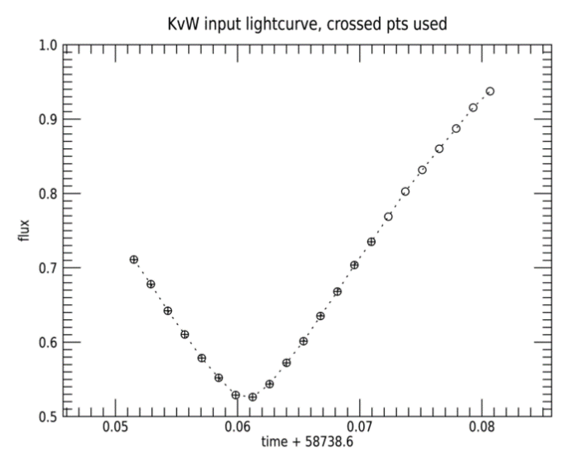
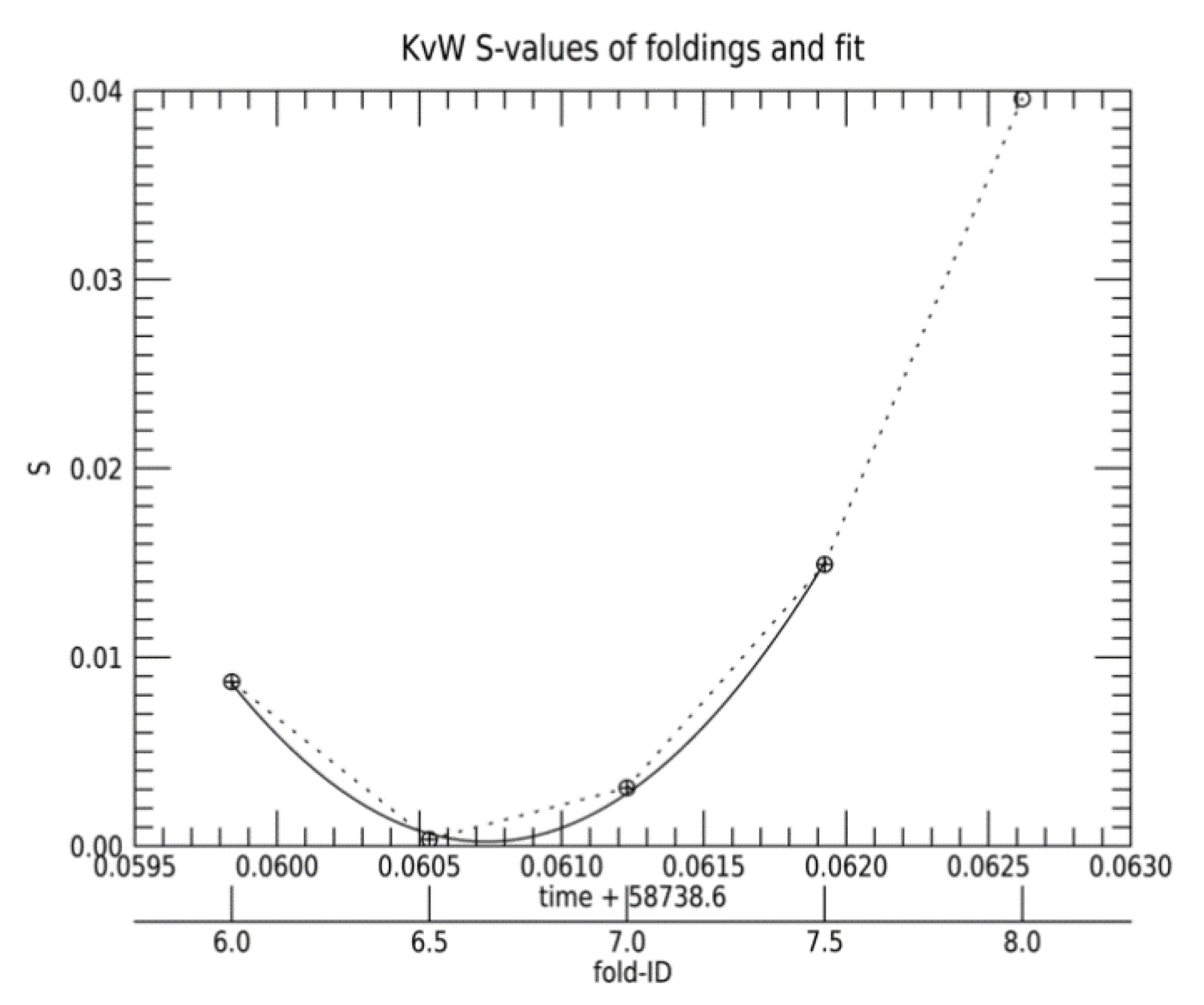
- Selection of data points: While the user has to take care that an input time-series only contains data collected during an eclipse (usually requiring a minimum flux-drop against the off-eclipse flux, see Figure 2), asymmetric data coverage around the center of an eclipse is recognized by the code. The code always selects the maximum number of data points that are available for pairings on either branch of an eclipse, and hence balances the coverage between the ingress and the egress (Figure 3);
- −
- Employment of more than three folds around the initial minimum time estimate: The number of folds needs to be odd and the use of five (default) or seven folds is recommended;
- −
- For the initial minimum time estimate, the algorithm uses—by default—the central point of the supplied light curve, but the user may also choose to use the point with the lowest flux. The central value is the better choice unless there are considerable asymmetries in the eclipse light curve. The point of the least flux should only be used in low-noise data, when this point is well-defined against the noise of the curve;
- −
- The code automatically selects the maximum amount of data points that can be paired for folds, which avoids errors when data of incomplete eclipses are provided (see Figure 3).
- −
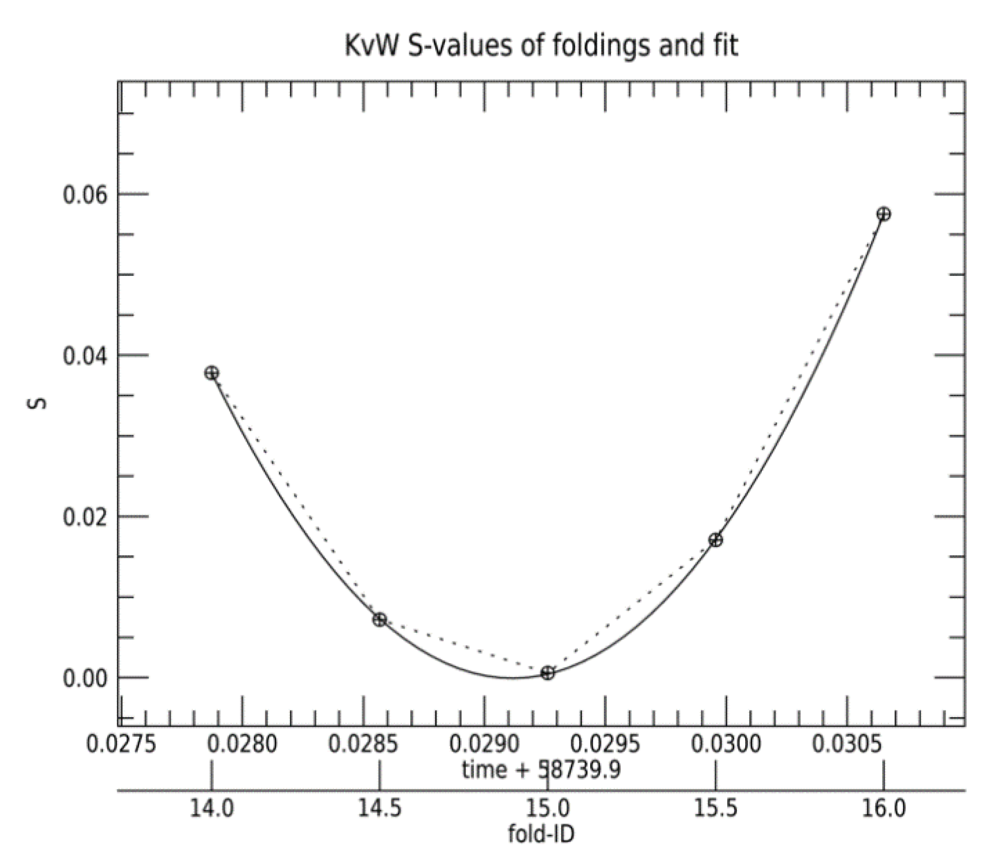
- Symmetrizing the fit to S(T): If the lowest value of S(T) does not correspond to a fold that is close to the initial estimate of the minimum time, the fitted curve Sfit will have branches of unequal length and the longer branch either to the left or right of the lowest S(T) has a larger weight for the coefficients a, b, and c. The same situation may also arise when data from incomplete eclipses are analyzed (see also Figure 4). As a remedy, the outer values of S(T) for the longer branch are cropped, so that this branch is at most one point larger than the shorter one. The fit for Sfit is then performed based on the reduced set of values S(T). This cropping can only be performed if S(T) has been obtained at more than three folds;
- −
- The code also permits a determination of the timing error using the original procedure of KvW from 1956, which does not require an explicit determination of the noise of the flux values;
- −
5. Example Application to TESS Data and Verification of the Error Estimates
6. Conclusions
Supplementary Materials
Funding
Data Availability Statement
Acknowledgments
Conflicts of Interest
Appendix A. Tables of CM Dra Minimum Times and Errors with Three and Seven Folds

| Epoch-Nr. | T0 | σT0 | σT0KvW |
|---|---|---|---|
| (BJD-TBD-2400000) | (10−5 d) | (10−5 d) | |
| Primary eclipses | |||
| 7024 | 58,739.9291143 | 1.23 | 1.05 |
| 7025 | 58,741.1975064 | 1.23 | 1.48 |
| 7026 | 58,742.4659164 | 1.24 | 1.89 |
| 7027 | 58,743.7342592 | 1.24 | 2.83 |
| 7028 | 58,745.0026685 | 1.23 | 1.40 |
| 7029 | 58,746.2710807 | 1.23 | 1.53 |
| 7030 | 58,747.5394642 | 1.25 | 1.84 |
| 7031 | 58,748.8078501 | 1.24 | 2.02 |
| 7032 | 58,750.0762641 | 1.23 | 1.31 |
| 7034 | 58,752.6130327 | 1.25 | 1.95 |
| 7035 | 58,753.8813901 | 1.23 | 1.87 |
| 7036 | 58,755.1498091 | 1.23 | 0.85 |
| 7037 | 58,756.4182183 | 1.24 | 1.78 |
| 7038 | 58,757.6866029 | 1.25 | 1.57 |
| 7039 | 58,758.9549792 | 1.24 | 1.86 |
| 7040 | 58,760.2233503 | 1.24 | 0.72 |
| 7041 | 58,761.4917561 | 1.23 | 1.45 |
| 7042 | 58,762.7601639 | 1.25 | 1.71 |
| Mean | 1.24 ± 0.01 | 1.62 ± 0.48 | |
| Secondary eclipses | |||
| 7023 | 58,739.2936082 | 1.32 | 1.93 |
| 7024 | 58,740.5619809 | 1.35 | NaN |
| 7025 | 58,741.8303809 | 1.32 | 1.74 |
| 7026 | 58,743.0987663 | 1.31 | 1.37 |
| 7027 | 58,744.3671520 | 1.32 | 1.93 |
| 7028 | 58,745.6355150 | 1.33 | 1.98 |
| 7029 | 58,746.9039464 | 1.31 | 1.18 |
| 7030 | 58,748.1723268 | 1.31 | 1.11 |
| 7031 | 58,749.4406646 | 1.36 | NaN |
| 7033 | 58,751.9775236 | 1.31 | 1.58 |
| 7034 | 58,753.2458785 | 1.31 | 1.14 |
| 7035 | 58,754.5142644 | 1.34 | 2.19 |
| 7036 | 58,755.7826500 | 1.32 | 1.75 |
| 7037 | 58,757.0510515 | 1.32 | 1.49 |
| 7038 | 58758.3194392 | 1.32 | 1.65 |
| 7039 | 58,759.5878394 | 1.32 | 1.86 |
| 7040 | 58,760.8562203 | 1.33 | 1.86 |
| 7041 | 58,762.1245984 | 1.31 | 1.30 |
| Mean | 1.32 ± 0.01 | 1.63 ± 0.33 | |
| Epoch-Nr. | T0 | σT0 | σT0KvW |
|---|---|---|---|
| (BJD-TBD-2400000) | (10−5 d) | (10−5 d) | |
| Primary eclipses | |||
| 7024 | 58,739.9291150 | 1.28 | 5.49 |
| 7025 | 58,741.1975027 | 1.28 | 5.7 |
| 7026 | 58,742.4659090 | 1.26 | 2.06 |
| 7027 | 58,743.7342707 | 1.26 | 0.88 |
| 7028 | 58,745.0026684 | 1.28 | 5.53 |
| 7029 | 58,746.2710792 | 1.28 | 5.63 |
| 7030 | 58,747.5394538 | 1.26 | 2.38 |
| 7031 | 58,748.8078483 | 1.26 | 2.69 |
| 7032 | 58,750.0762621 | 1.28 | 5.43 |
| 7034 | 58,752.6130182 | 1.26 | 2.23 |
| 7035 | 58,753.8813882 | 1.26 | 2.97 |
| 7036 | 58,755.1498096 | 1.28 | 5.48 |
| 7037 | 58,756.4182146 | 1.29 | 5.67 |
| 7038 | 58,757.6865875 | 1.27 | 2.07 |
| 7039 | 58,758.9549780 | 1.26 | 2.61 |
| 7040 | 58,760.2233496 | 1.29 | 5.51 |
| 7041 | 58,761.4917544 | 1.28 | 5.77 |
| 7042 | 58,762.7601513 | 1.26 | 1.95 |
| Mean | 1.27 ± 0.01 | 3.89 ± 1.79 | |
| Secondary eclipses | |||
| 7023 | 58,739.2936076 | 1.35 | 2.67 |
| 7024 | 58,740.5619515 | 1.35 | 1.62 |
| 7025 | 58,741.8303818 | 1.37 | 5.51 |
| 7026 | 58,743.0987636 | 1.36 | 5.45 |
| 7027 | 58,744.3671522 | 1.35 | 2.27 |
| 7028 | 58,745.6355255 | 1.35 | 2.02 |
| 7029 | 58,746.9039487 | 1.37 | 5.49 |
| 7030 | 58,748.1723265 | 1.36 | 5.42 |
| 7031 | 58,749.4407207 | 1.35 | 2.45 |
| 7033 | 58,751.9775250 | 1.36 | 5.41 |
| 7034 | 58,753.2458815 | 1.37 | 5.32 |
| 7035 | 58,754.5142620 | 1.36 | 1.81 |
| 7036 | 58,755.7826560 | 1.35 | 2.33 |
| 7037 | 58,757.0510536 | 1.37 | 5.65 |
| 7038 | 58,758.3194397 | 1.37 | 5.06 |
| 7039 | 58,759.5878375 | 1.35 | 2.01 |
| 7040 | 58,760.8562260 | 1.35 | 2.09 |
| 7041 | 58,762.1245984 | 1.36 | 5.51 |
| Mean | 1.36 ± 0.01 | 3.78 ± 1.71 | |
References
- Kwee, K.K.; van Woerden, H. A method for computing accurately the epoch of minimum of an eclipsing variable. Bull. Astron. Inst. Netherlands 1956, 12, 327–330. [Google Scholar]
- Mikulášek, Z.; Wolf, M.; Zejda, M.; Pecharová, P. On methods for the light curves extrema determination. In Close Binaries in the 21st Century: New Opportunities and Challenges; Springer: Dordrecht, The Netherlands, 2006; pp. 363–365. [Google Scholar]
- Mikulášek, Z.; Chrastina, M.; Liška, J.; Zejda, M.; Janík, J.; Zhu, L.-Y.; Qian, S.-B. Kwee-van Woerden method: To use or not to use. Contr. Astr. Obs. Skalnaté Pleso 2014, 43, 382–387. [Google Scholar]
- Breinhorst, R.A.; Pfleiderer, J.; Reinhardt, M.; Karimie, M.T. On the determination of minimum times of light curves. Astron. Astrophys. 1973, 22, 239–245. [Google Scholar]
- Morales, J.C.; Ribas, I.; Jordi, C.; Torres, G.; Gallardo, J.; Guinan, E.F.; Charbonneau, D.; Wolf, M.; Latham, D.W.; Anglada-Escudé, G.; et al. Absolute properties of the low-mass eclipsing binary CM Draconis. Astrophys. J. 2009, 691, 1400–1411. [Google Scholar] [CrossRef]
- Ricker, G.R.; Latham, D.W.; Vanderspek, R.K.; Ennico, K.A.; Bakos, G.; Brown, T.M.; Burgasser, A.J.; Charbonneau, D.; Christensen-Dalsgaard, J.; Clampin, M.; et al. Transiting Exoplanet Survey Satellite (TESS). J. Astron. Telesc. Instr. Sys. 2015, 1, 014003. [Google Scholar] [CrossRef] [Green Version]
- Memo to TESS Data Release Note 29. Available online: https://archive.stsci.edu/missions/tess/doc/tess_drn/tess_s21_dr29_data_product_revision_memo_v02.pdf (accessed on 16 November 2020).
- Tenenbaum, P.; Jenkins, J. TESS Science Data Products Description Document, EXP-TESS-ARC-ICD-0014 Rev D; NASA Technical Report; 2018. Available online: https://ntrs.nasa.gov/api/citations/20180007935/downloads/20180007935.pdf (accessed on 1 December 2020).
- Deeg, H.J.; Ocaña, B.; Kozhevnikov, V.P.; Charbonneau, D.; O’Donovan, F.T.; Doyle, L.R. Extrasolar planet detection by binary stellar eclipse timing: Evidence for a third body around CM Draconis. Astron. Astrophys. 2008, 480, 563–571. [Google Scholar] [CrossRef]
- Deeg, H.J.; Tingley, B. TEE, an estimator for the precision of eclipse and transit minimum times. Astron. Astrophys. 2017, 599, A93. [Google Scholar] [CrossRef] [Green Version]


| Epoch Nr. | T0 | σT0 | σT0KvW |
|---|---|---|---|
| (BJD-TBD-2400000) | (10−5 d) | (10−5 d) | |
| Primary eclipses | |||
| 7024 | 58,739.9291169 | 1.25 | NaN |
| 7025 | 58,741.1975015 | 1.25 | NaN |
| 7026 | 58,742.4659011 | 1.26 | 2.78 |
| 7027 | 58,743.7342864 | 1.26 | 2.20 |
| 7028 | 58,745.0026702 | 1.25 | NaN |
| 7029 | 58,746.2710774 | 1.25 | NaN |
| 7030 | 58,747.5394452 | 1.26 | 2.81 |
| 7031 | 58,748.8078623 | 1.26 | 2.19 |
| 7032 | 58,750.0762635 | 1.25 | NaN |
| 7034 | 58,752.6130101 | 1.26 | 2.85 |
| 7035 | 58,753.8813997 | 1.25 | 2.06 |
| 7036 | 58,755.1498107 | 1.25 | NaN |
| 7037 | 58,756.4182122 | 1.25 | NaN |
| 7038 | 58,757.6865806 | 1.27 | 2.81 |
| 7039 | 58,758.9549907 | 1.26 | 1.90 |
| 7040 | 58,760.2233508 | 1.26 | NaN |
| 7041 | 58,761.4917508 | 1.24 | NaN |
| 7042 | 58,762.7601436 | 1.26 | 2.86 |
| Mean | 1.25 ± 0.01 | 2.50 ± 0.40 | |
| Secondary eclipses | |||
| 7023 | 58,739.2935944 | 1.34 | 2.23 |
| 7024 | 58,740.5619511 | 1.36 | 3.23 |
| 7025 | 58,741.8303857 | 1.34 | NaN |
| 7026 | 58,743.0987637 | 1.33 | NaN |
| 7027 | 58,744.3671428 | 1.35 | 2.18 |
| 7028 | 58,745.6355326 | 1.35 | 2.95 |
| 7029 | 58,746.9039510 | 1.33 | NaN |
| 7030 | 58,748.1723260 | 1.33 | NaN |
| 7031 | 58,749.4407154 | 1.36 | 3.78 |
| 7033 | 58,751.9775280 | 1.33 | NaN |
| 7034 | 58,753.2458785 | 1.33 | NaN |
| 7035 | 58,754.5142489 | 1.36 | 2.34 |
| 7036 | 58,755.7826651 | 1.34 | 2.75 |
| 7037 | 58,757.0510572 | 1.34 | NaN |
| 7038 | 58,758.3194374 | 1.34 | NaN |
| 7039 | 58,759.5878263 | 1.35 | 2.32 |
| 7040 | 58,760.8562353 | 1.35 | 2.58 |
| 7041 | 58,762.1246012 | 1.33 | NaN |
| Mean | 1.34 ± 0.01 | 2.71 ± 0.53 | |
| Description | σT0,prim | σT0,sec |
|---|---|---|
| (10−5 d) | (10−5 d) | |
| Three-fold KvW method | ||
| Timing errors of individual eclipses, KvW original calculation | 1.62 ± 0.48 | 1.63 ± 0.33 1 |
| Ditto, revised calculation | 1.24 ± 0.01 | 1.32 ± 0.01 |
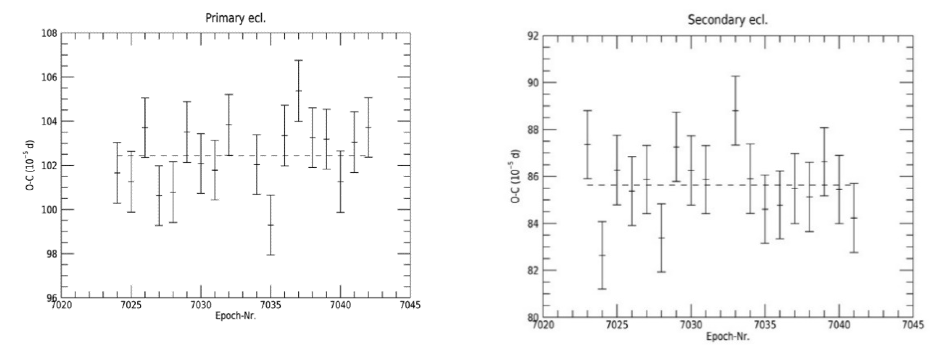
| Standard dev. of minimum times against mean O-C value | 1.60 | 1.65 |
| Five-fold KvW method | ||
| Timing errors of individual eclipses, KvW original calculation | 2.50 ± 0.40 2 | 2.71 ± 0.53 2 |
| Ditto, revised calculation | 1.25 ± 0.01 | 1.34 ± 0.01 |
| Standard dev. of minimum times against mean O-C value | 1.18 | 1.48 |
| Seven-fold KvW method | ||
| Timing errors of individual eclipses, KvW original calculation | 3.89 ± 1.79 | 3.78 ± 1.71 |
| Ditto, revised calculation | 1.27 ± 0.01 | 1.36 ± 0.01 |
| Standard dev. of minimum times against mean O-C value | 1.28 | 1.36 |
| Timing Error Estimator (TEE), from [10] | 1.21 | 1.29 |
Publisher’s Note: MDPI stays neutral with regard to jurisdictional claims in published maps and institutional affiliations. |
© 2020 by the author. Licensee MDPI, Basel, Switzerland. This article is an open access article distributed under the terms and conditions of the Creative Commons Attribution (CC BY) license (http://creativecommons.org/licenses/by/4.0/).
Share and Cite
Deeg, H.J. A Modified Kwee–Van Woerden Method for Eclipse Minimum Timing with Reliable Error Estimates. Galaxies 2021, 9, 1. https://doi.org/10.3390/galaxies9010001
Deeg HJ. A Modified Kwee–Van Woerden Method for Eclipse Minimum Timing with Reliable Error Estimates. Galaxies. 2021; 9(1):1. https://doi.org/10.3390/galaxies9010001
Chicago/Turabian StyleDeeg, Hans J. 2021. "A Modified Kwee–Van Woerden Method for Eclipse Minimum Timing with Reliable Error Estimates" Galaxies 9, no. 1: 1. https://doi.org/10.3390/galaxies9010001
APA StyleDeeg, H. J. (2021). A Modified Kwee–Van Woerden Method for Eclipse Minimum Timing with Reliable Error Estimates. Galaxies, 9(1), 1. https://doi.org/10.3390/galaxies9010001