Analysing Hubble Tension and Gravitational Waves for f(Q,T) Gravity Theories

Abstract

In this work, we examine viable models of $f(Q,T)$ gravity theories against observational data with the aim to constrain the parameter space of these models. We have analyzed four different models of $f(Q,T)$ gravity and tested them against against late-time background probes: Cosmic Chronometer (CC), Baryon Acoustic Oscillations (DESI BAO), $Pantheo{n}^{+}$ and Gravitational wave(GWTC-3) data. We put stringent constraints on the $f(Q,T)$ gravity models, $f(Q,T)=\alpha Q+\beta T$, $f(Q,T)=\alpha Q^n+\beta T$, $f(Q,T)=-\alpha Q-\beta T^2$ and $f(Q,T)=\alpha Q^{-2}{T}^2$ along with other late-time cosmological parameters such as deceleration parameter ($q_0$), equation of state parameter ($w_0$), sound horizon distance ($r_d$) and demonstrate their alignment with the $\mathrm{\Lambda }CDM$ model and the observational data. We show that these models have the capability to alleviate the Hubble tension in late time universe, by predicting the present value of the Hubble parameter close to 74 km/s/Mpc. $f(Q,T)$ gravity theory introduces alterations in the background evolution and imposes a friction term in the propagation of gravitational waves, this phenomenon has also been examined. We have shown their agreement with the Gravitational Wave (GW) luminosity distance with the Electromagnetic (EM) counter part GWTC-3 data from Advanced LIGO and Advanced VIRGO across different observing runs capturing coalescence of Binary Neutron Stars (BNS), mergers of Binary Black Holes (BBHs), and Neutron Star-Black Hole (NSBH) binaries with EM counterparts.

1. Introduction

In recent years, precision cosmology has revealed several statistically significant discrepancies-commonly known as cosmic tensions-between early and late-time observational datasets. These tensions challenge the validity of the standard $\mathrm{\Lambda }$CDM model and suggest that new physics may be necessary to fully explain the evolution of the universe.

The most widely discussed is the Hubble tension, which refers to the inconsistency in the inferred value of the present-day Hubble parameter $H_0$. The Planck 2018 results based on cosmic microwave background (CMB) measurements estimate $H_0=67.4\pm 0.5$ km/s/Mpc [1], assuming the $\mathrm{\Lambda }$CDM model. In contrast, direct measurements from the local universe, such as those from the SH0ES project [2] and the compilation $Pantheo{n}^{+}$ [3], report a significantly higher value around $74.03\pm 1.42$ km/s/Mpc. The tension exceeds the level $5\sigma$ and persists in multiple independent methods, indicating a potential breakdown in our cosmological model.

Another notable inconsistency is the $S_8$ tension, which pertains to the amplitude of matter fluctuations on scales of 8 $h^{-1}$ Mpc. Weak lensing surveys, including KiDS-1000 [4] and DESI [5], favor lower values of $S_8={\sigma }_8\sqrt{{\mathrm{\Omega }}_m/0.3}$ compared to those inferred from Planck CMB data [6,7]. This suggests a slower growth of cosmic structures in the late universe than predicted by $\mathrm{\Lambda }$CDM.

Baryon Acoustic Oscillations (BAO) also introduce subtler tensions. Although BAO data generally agree with the predictions of $\mathrm{\Lambda }$CDM, recent analyses suggest potential early dark energy (EDE) signatures [8,9], which could partially resolve the $H_0$ tension but introduce new challenges, such as inconsistencies in the CMB damping tail and the matter power spectrum.

There is also a growing discussion about the so-called cosmic curvature tension. While CMB data strongly support a spatially flat universe, some combinations of late-time observables (like strong lensing and BAO) mildly favor a closed universe [10,11]. Though less statistically significant, this points again to potential shortcomings in the standard model.

These persistent tensions have led to renewed interest in alternative models of gravity. One promising class involves modified gravity theories that extend General Relativity (GR) by modifying either the matter sector or the geometric structure of spacetime.Among these, $f(Q,T)$ gravity has garnered attention as a extension of symmetric teleparallel gravity, where the gravitational Lagrangian depends on both the non-metricity scalar Q and the trace T of the energy-momentum tensor [12]. This theory resides in the non-Riemannian formulation of gravity, where spacetime geometry is encoded in non-metricity rather than curvature or torsion. Starting from the given gravitational Lagrangian, one can construct the geometric action in the standard way. Varying this action with respect to the metric tensor yields the general field equations for gravity in the presence of geometry–matter coupling. The study further explores the cosmological consequences of the $f(Q,T)$ theory [13,14,15], suggesting that $f(Q,T)$ gravity offers valuable perspectives for understanding the dynamics of the Universe in both its early and late stages.

A distinguishing feature of $f(Q,T)$ gravity is its natural violation of the energy-momentum conservation law, resulting from the explicit coupling between matter and geometry. This non-conservation introduces an extra force that can affect the motion of test particles and mimic effects usually attributed to dark energy or modified matter content. Any realistic study of this theory must consider this feature, as it fundamentally alters the cosmic dynamics and perturbation evolution.

In this work, we investigate whether $f(Q,T)$ gravity models can alleviate the Hubble tension in late-time universe and simultaneously remain consistent with other late-time cosmological probes. We test several functional forms of $f(Q,T)$ against a comprehensive set of late-time observations, including Cosmic Chronometers, Baryon Acoustic Oscillations, $Pantheo{n}^{+}$ and recent gravitational wave standard siren data from the GWTC-3 catalog. We also study the impact of $f(Q,T)$ on gravitational wave propagation, focusing on its implications for the GW luminosity distance and the friction term in the evolution of tensor mode. We further test the distance duality relation (DDR) for our class of $f(Q,T)$ theories.

The plan of our work is the following. In Section 2, we briefly review the $f(Q,T)$ gravity theory and discuss the modified background and gravitational wave equations. In Section 3 we discuss the various datasets with which we have worked in this paper together with our data analysis technique. We have also discussed the model comparison criteria to verify our models according to the Akaike Information Criterion (AIC), $\Delta AIC$ and the Bayesian or Schwarz information criterion (BIC), $\Delta BIC$. Then in Section 4 we have analyzed different $f(Q,T)$ models against the Hubble tension and GW. In Section 5 we have discussed the comparison of our models with reference model($\mathrm{\Lambda }CDM$), tested the DDR. Finally, in Section 6, we conclude.

2. f (Q, T) Gravity Theory

$f(Q,T)$ gravity was originally proposed by [16]. Here, the gravitational action $\mathcal{L}$ is determined by an arbitrary function f which depends on both the non-metricity scalar Q and the trace of the matter energy-momentum tensor T. The overall action for $f(Q,T)$ gravity [16] is expressed as:

$$S=\int d^{4}x\sqrt{-g}\left({\displaystyle \frac{1}{2k}}f(Q,T)+{\mathcal{L}}_m\right)$$

(1)

where ${\mathcal{L}}_m$ for the matter Lagrangian and g for the determinant of the metric. We adopt the following convention: $k=8\pi G$ and $G=1$. Q, the non-metricity scalar [17], is defined as,

$$Q=-g^{\alpha \beta }(L_{\delta \alpha }^{\gamma }{L}_{\beta \gamma }^{\delta }-L_{\delta \gamma }^{\gamma }{L}_{\alpha \beta }^{\delta })$$

(2)

where $L_{\delta \alpha }^{\gamma }$ is the deformation tensor [16] given by,

$$L_{\delta \alpha }^{\gamma }=-{\displaystyle \frac{1}{2}}{g}^{\gamma \lambda }({\nabla }_{\alpha }{g}_{\delta \lambda }+{\nabla }_{\delta }{g}_{\lambda \alpha }-{\nabla }_{\lambda }{g}_{\beta \delta })$$

(3)

By varying the action in Equation (1) w.r.t the components of the metric tensor, we obtain the field equations [16] of the $f(Q,T)$ gravity theory as,

$$\begin{array}{c}\hfill -{\displaystyle \frac{2}{\sqrt{-g}}}{\nabla }_{\gamma }\left(f_Q\sqrt{-g}{P}_{\beta \alpha }^{\gamma }\right)-{\displaystyle \frac{1}{2}}f{g}_{\alpha \beta }+f_T(T_{\alpha \beta }+{\Theta }_{\alpha \beta })\\ \hfill -f_Q(P_{\alpha \gamma \delta }{Q}_{\beta }^{\gamma \delta }-2Q_{\alpha }^{\gamma \delta }{P}_{\gamma \delta \beta })=8\pi T_{\alpha \beta }\end{array}$$

(4)

where, $Q_{\beta \alpha \gamma }={\nabla }_{\beta }{g}_{\alpha \gamma }$ is the non-metricity tensor, $f_Q={\displaystyle \frac{\partial f}{\partial Q}}$, $f_T={\displaystyle \frac{\partial f}{\partial T}}$, $T_{\alpha \beta }=-{\displaystyle \frac{2}{\sqrt{-g}}}{\displaystyle \frac{\delta \left(\sqrt{-g}{L}_m\right)}{\delta g^{\alpha \beta }}}$.

The stress-energy tensor, ${\mathrm{\Theta }}_{\alpha \beta }=g^{\gamma \delta }{\displaystyle \frac{\delta T_{\gamma \delta }}{\delta g^{\alpha \beta }}}$ and $P_{\alpha \beta }^{\gamma }$ is the super potential that is given by, [16]

$$P_{\alpha \beta }^{\gamma }=-{\displaystyle \frac{1}{2}}{L}_{\alpha \beta }^{\gamma }+{\displaystyle \frac{1}{4}}\left(Q^{\gamma }-{\tilde{Q}}^{\gamma }\right)g_{\alpha \beta }-{\displaystyle \frac{1}{4}}{\delta }_{(\alpha }^{\gamma }{Q}_{\beta )}$$

(5)

where, $Q_{\gamma }\equiv Q_{\gamma \delta }^{\delta }$ and ${\tilde{Q}}_{\gamma }={\tilde{Q}}_{\gamma \delta }^{\delta }$

In terms of super potential, the non-metricity scalar can be defined as, $Q=-Q_{\alpha \beta \gamma }{P}^{\alpha \beta \gamma }$.

Additionally, the hyper-momentum tensor density is defined as follows:

$$H_{\lambda }^{\alpha \beta }\equiv {\displaystyle \frac{\sqrt{-g}}{2k}}{f}_T{\displaystyle \frac{\delta T}{\delta {\mathrm{\Gamma }}_{\alpha \beta }^{\lambda }}}+{\displaystyle \frac{\delta \sqrt{-g}{\mathcal{L}}_m}{\delta {\mathrm{\Gamma }}_{\alpha \beta }^{\lambda }}}$$

(6)

Thus, the field equations are derived by varying the gravitational action with respect to the connection.

$${\nabla }_{\alpha }{\nabla }_{\beta }\left(\sqrt{-g}{f}_Q{P}^{\alpha \beta }+{\displaystyle \frac{1}{2}}k{H}_{\gamma }^{\alpha \beta }\right)=0$$

(7)

The metric divergence field equation is given by [16],

$$\begin{array}{c}\hfill {\mathcal{D}}_{\alpha }\left[f_T(T_{\beta }^{\alpha }+{\mathrm{\Theta }}_{\beta }^{\alpha })-8\pi T_{\beta }^{\alpha }\right]+{\displaystyle \frac{8\pi }{\sqrt{-g}}}{\nabla }_{\gamma }{\nabla }_{\alpha }{H}_{\beta }^{\gamma \beta }\\ \hfill ={\displaystyle \frac{1}{2}}{f}_T{\partial }_{\beta }T+{\displaystyle \frac{1}{\sqrt{-g}}}{Q}_{\alpha }{\nabla }_{\alpha }\left(f_Q\sqrt{-g}{P}_{\gamma }^{\alpha \beta }\right)\end{array}$$

(8)

Additionally, we solve Equation (7) by introducing a tensor $A_{\beta }^{\alpha }$. so that

$${\nabla }_{\alpha }\left(\sqrt{-g}{f}_Q{P}_{\gamma }^{\alpha \beta }+{\displaystyle \frac{1}{2}}k{H}_{\gamma }^{\alpha \beta }\right)=\sqrt{-g}{A}_{\gamma }^{\alpha }$$

(9)

where there is an additional constraint that is,

$${\nabla }_{\beta }\left(\sqrt{-g}{A}_{\gamma }^{\alpha }\right)={\displaystyle \frac{\sqrt{-g}}{2}}{Q}_{\alpha }{A}_{\gamma }^{\alpha }+\sqrt{-g}{\nabla }_{\alpha }^{\gamma }=0$$

(10)

By using Equations (8) and (9) it is worth noting that the divergence of the matter energy-momentum tensor in the $f(Q,T)$ theory can be expressed as follows,

$$\begin{array}{c}\hfill {\mathcal{D}}_{\alpha }{T}_{\beta }^{\alpha }={\displaystyle \frac{1}{f_T-\kappa }}[-{\mathcal{D}}_{\alpha }\left(f_T{\mathrm{\Theta }}_{\beta }^{\alpha }\right)-{\displaystyle \frac{2k}{\sqrt{-g}}}{\nabla }_{\gamma }{\nabla }_{\alpha }{H}_{\beta }^{\gamma \beta }\\ \hfill +\kappa {\nabla }_{\alpha }\left({\displaystyle \frac{1}{\sqrt{-g}}}{\nabla }_{\gamma }{H}_{\beta }^{\gamma \alpha }\right)-2{\nabla }_{\alpha }{A}_{\beta }^{\alpha }+{\displaystyle \frac{1}{2}}{f}_T{\partial }_{\beta }T]=B_{\beta }\end{array}$$

(11)

In the framework of $f(Q,T)$ gravity, the non-conservation vector $B_{\beta }$ is influenced by both the non-metricity scalar Q, the trace of the energy-momentum tensor T.

As a result, the matter energy-momentum tensor is not conserved, expressed as ${\mathcal{D}}_{\alpha }{T}_{\beta }^{\alpha }=B_{\beta }\ne 0$. This violation of conservation implies the presence of an additional force acting on massive test particles, causing their trajectories to deviate from geodesic paths. Such behavior reflects an exchange of energy within a given volume, pointing to processes like energy transfer or particle creation occurring in the system [16]. In particular, when the $f_T$ terms vanish, the right-hand side becomes zero, restoring the conservation of the energy-momentum tensor [17].

2.1. Evolution of the Friedmann Equations

To derive the Friedmann equations, which describe the evolution of the universe, we start by assuming that the universe’s matter content can be modeled as a perfect fluid. This perfect fluid is characterized by an energy-momentum tensor, which encapsulates the fluid’s density, pressure, and the dynamics of it is given by, $T_{\beta }^{\alpha }=diag(-\rho ,p,p,p)$. We work in the coincident gauge with the affine connection reduced to zero. In this gauge, using diffeomorphism gauge equality, we set the lapse function $N=1$. Working in the coincident gauge reduces the covariant derivatives to the standard ones. The non-metricity function Q for such a metric is calculated and obtained as $Q=6H^2$. The coincident gauge makes this relation trivial. Then for the tensor ${\mathrm{\Theta }}_{\beta }^{\alpha }$ we obtain the expression,

$${\mathrm{\Theta }}_{\beta }^{\alpha }={\delta }_{\beta }^{\alpha }p-2T_{\beta }^{\alpha }=diag(2\rho +p,-p,-p,-p)$$

(12)

Now, the mathematical notations regarding this gravity model are

$$F\equiv f_Q$$

(13)

and,

$$8\pi \tilde{G}\equiv f_T$$

(14)

where $f_Q$ denotes the derivative w.r.t. non-metricity Q and $f_T$ denotes the derivative w.r.t. trace of energy-momentum tensor T. In our assumed models, Model I and III has constant $f_Q$. But Model II and IV has a functional form. Now, for studying the background dynamics, we consider the Friedmann-Lemaitre-Robertson-Walker(FLRW) metric, given as

$$d{s}^2=-d{t}^2+a^2\left(t\right)\left[d{x}^2+d{y}^2+d{z}^2\right]$$

(15)

where, $a\left(t\right)$ is the scale factor, which is a function of cosmic time. From the field equations, we can easily find the Friedmann equations for $f(Q,T)$ gravity as [16],

$$8\pi \rho ={\displaystyle \frac{f}{2}}-6F{H}^2-{\displaystyle \frac{2\tilde{G}}{1+\tilde{G}}}(\dot{F}H+F\dot{H})$$

(16)

$$8\pi p=-{\displaystyle \frac{f}{2}}+6F{H}^2+2(\dot{F}H+F\dot{H})$$

(17)

Combining the preceding two equations will give the evolutionary equation for the Hubble function $H\left(t\right)$, expressed as follows:

$$\dot{H}+{\displaystyle \frac{\dot{F}}{F}}H={\displaystyle \frac{4\pi }{F}}(1+\tilde{G})(\rho +p)$$

(18)

To ensure broad applicability, we’ll adopt a cosmological matter model governed by an equation of state represented as

$$p=\omega \rho$$

(19)

where $\omega$ is equation of state parameter. This linear equation of state can describe the behavior of baryonic matter across varying densities, allowing it to describe conditions from the high-density scenarios akin to the early universe to the low-density conditions characteristic of the contemporary universe.

Combining Equation (19), Equations (16) and (18) we find the general expression for the matter density as,

$$\rho ={\displaystyle \frac{f-12F{H}^2}{16\pi [1+(1+\omega )\tilde{G}]}}$$

(20)

To obtain the cosmological outcomes that directly align model predictions with observations, we introduce an independent variable, the redshift z, instead of the time variable t, defined according to,

$$1+z={\displaystyle \frac{1}{a}}$$

(21)

where we have assumed the present day value of scale factor as $a_0=1$. Therefore the following relation now holds true,

$${\displaystyle \frac{d}{dt}}=-(1+z)H\left(z\right){\displaystyle \frac{d}{dz}}$$

(22)

By using this relation, we will find the evolution of the cosmological parameters w.r.t. redshift. From Equation (18) the evolution of Hubble parameter w.r.t. redshift is given by,

$${\displaystyle \frac{dH}{dz}}={\displaystyle \frac{\dot{F}H-4\pi (1+\omega )(1+\tilde{G})\rho }{(1+z)H\left(z\right)F}}$$

(23)

2.2. GW Propagation in f(Q,T) Gravity

To proceed, let us first recall the free propagation of tensor perturbations in GR, in a FLRW background is described by [18],

$$h_A^{″}+2\mathcal{H}{h}_A^{\prime }+{\kappa }^2{h}_A=0$$

(24)

where $h_A(\eta ,\kappa )$ is the Fourier mode of the Gravitational Wave(GW) amplitude, A in the suffix denotes the two polarization states + and × of the GWs, $\eta$ denotes the conformal time and $\mathcal{H}=a^{\prime }/a$ represents the conformal Hubble parameter. We further introduce a field ${\chi }_A(\eta ,k)$ through the following conformal transformation [19],

$$h_A(\eta ,\kappa )={\displaystyle \frac{1}{a\left(\eta \right)}}{\chi }_A(\eta ,\kappa )$$

(25)

So, Equation (24) becomes,

$${\chi }_A^{″}+({\kappa }^2-a^{″}/a){\chi }_A=0$$

(26)

Both in matter dominance and in the recent Dark Energy dominated epoch $a^{″}/a\approx 1/{\eta }^2$. For sub-horizon modes $\kappa \eta >>1$, and therefore $a^{″}/a$ can be neglected compared to ${\kappa }^2$.

$${\chi }_A^{″}+{\kappa }^2{\chi }_A=0$$

(27)

This indicates that the dispersion relation for tensor perturbations is $\omega =\kappa$, meaning that GWs propagate at the speed of light. The factor $1/a$ in Equation (25) illustrates how the amplitude of GWs diminishes as they travel over cosmological distances from their source to the observer. For inspiralling binaries, this results in the standard relationship between the GW amplitude and the luminosity distance, expressed as $h_A(\eta ,\kappa )\propto 1/d_L\left(z\right)$. Altering the coefficient of the ${\kappa }^2$ term in Equation (24) would change the propagation speed of GWs relative to the speed of light. However, the GW170817/GRB 170817A event has placed a stringent limit on such modifications, with $|c_{gw}-c|/c<\mathcal{O}\left({10}^{-15}\right)$ [20], effectively ruling out a significant portion of scalar-tensor and vector-tensor modifications of GR [21,22,23,24].

Now, let’s explore the propagation of GWs in $f(Q,T)$ gravity which is similar to one in $f\left(Q\right)$ gravity. This was expected since in vacuum the energy-momentum tensor is zero. This similarity arises because, in a vacuum, the energy-momentum tensor vanishes, leading to a zero trace of the energy-momentum tensor $(T=0)$. For a perturbed ‘Einstein-Hilbert’ action and the energy-momentum tensor expanded to the second order in the metric, within the context of the FLRW background metric, the behavior of GWs in $f(Q,T)$ gravity,

$$g_{\mu \nu }=a^2\left(\eta \right)diag(-1,1,1,1)$$

(28)

and by considering the TT gauge in Equation (24), the propagation equation for GWs in $f(Q,T)$ gravity will be, [19,25]

$$h_A^{″}+2\mathcal{H}\left[1-\delta \left(\eta \right)\right]h_A^{\prime }+{\kappa }^2{h}_A=0$$

(29)

where $\delta \left(\eta \right)$ parametrizes the deviation from GR (also known as the friction term), which reads as

$$\delta \left(\eta \right)={\displaystyle \frac{1}{2\mathcal{H}}}{\displaystyle \frac{d\left(log{f}_Q\right)}{d\eta }}$$

(30)

Like before, we introduce ${\chi }_A(\eta ,\kappa )$ as

$$h_A(\eta ,\kappa )={\displaystyle \frac{1}{\tilde{a}\left(\eta \right)}}{\chi }_A(\eta ,\kappa )$$

(31)

and we get

$${\chi }_A^{″}+({\kappa }^2-{\tilde{a}}^{″}/\tilde{a}){\chi }_A=0$$

(32)

Again, the term ${\tilde{a}}^{″}/\tilde{a}$ is negligible inside the horizon, so GWs propagate at the speed of light. $\tilde{a}$ is a modified or rescaled version of the scale factor, which appears in the equation to account for the effects of the universe’s expansion on the perturbation ${\chi }_A$. However, while propagating over cosmological distances, $h_A$ now decreases as $1/\tilde{a}$ rather than $1/a$. The friction term present in Equation (29) alters the evolution of GW amplitude as it propagates through cosmological distances. In GR, the amplitude of a coalescing binary is inversely proportional to the luminosity distance as, $1/d_L$. This relationship causes a bias in the inferred luminosity distance derived from GW observations. Specifically, if $\delta \left(\eta \right)<0$, the damping term is stronger, causing the GW amplitude to decrease more significantly during propagation from the source to the detector. Within the framework of GR, this would lead to the erroneous interpretation that the source is farther away than it actually is. Conversely, if $\delta \left(\eta \right)>0$, the GW amplitude would appear larger, suggesting a source distance that is closer than its true distance. Therefore, it is essential to distinguish between two types of luminosity distances: the ‘electromagnetic luminosity distance’, denoted as $d_L^{em}$, and the ‘GW luminosity distance’, denoted as $d_L^{gw}$. Then in such a modified gravity model, for a coalescing binary at redshift z, the two are now related as, [19,25]

$$d_L^{gw}\left(z\right)={\displaystyle \frac{a\left(z\right)}{\tilde{a}\left(z\right)}}{d}_L^{em}={\displaystyle \frac{1}{(1+z)\tilde{a}\left(z\right)}}{d}_L^{em}$$

(33)

By substituting the scale factor $\mathcal{H}[1-\delta \left(\eta \right)]={\displaystyle \frac{\widetilde{a^{\prime }}}{\tilde{a}}}$ and performing some straightforward calculation, we can redefine the relation between GW luminosity distance and EM luminosity distance as, [19,25]

$$d_L^{gw}=d_L^{em}exp\left(-{\int }_0^z{\displaystyle \frac{\delta \left(z^{\prime }\right)d{z}^{\prime }}{(1+z^{\prime })}}\right)$$

(34)

Thus we see that the difference between the two types of luminosity distances now depends on the friction term which directly depends on the corresponding modified gravity model. By quantifying deviations of the GW luminosity distance concerning the electromagnetic luminosity distance, we would be able to measure deviations from GR.

In $f(Q,T)$ gravity model, the above relation takes the form, [18]

$$d_L^{gw}=\sqrt{{\displaystyle \frac{f_Q\left(0\right)}{f_Q}}}{d}_L^{em}$$

(35)

Here $f_Q\left(0\right)$ is a function $f_Q$ computed at present time i.e., $z=0$. From the above equation and using EM wave luminosity distance

$$d_L^{em}\left(z\right)=c(1+z){\int }_0^z{\displaystyle \frac{d{z}^{\prime }}{H\left(z^{\prime }\right)}}$$

(36)

We can obtain the expression of $d_L^{gw}$ in terms of redshift z. as,

$$d_L^{gw}=c(1+z)\sqrt{{\displaystyle \frac{f_Q\left(0\right)}{f_Q}}}{\int }_0^z{\displaystyle \frac{d{z}^{\prime }}{H\left(z^{\prime }\right)}}$$

(37)

2.3. The Distance Duality Relation

The angular-diameter distance $d_A$ is defined such that the angular size $\theta$ of an object, which spans a proper length s perpendicular to the line of sight, follows the standard Euclidean formula,

$$\theta ={\displaystyle \frac{s}{d_A}}$$

(38)

In a FLRW universe, the proper distance s associated with an angular separation $\theta$ is given by,

$$s=a\left(t\right)r\theta ={\displaystyle \frac{r\theta }{1+z}}$$

(39)

where the scale factor is unity for the present time. So, the angular-diameter distance will be,

$$d_A={\displaystyle \frac{c}{1+z}}{\int }_0^z{\displaystyle \frac{d{z}^{\prime }}{H\left(z^{\prime }\right)}}$$

(40)

Now, comparing Equations (37) and (40), one finds,

$${\displaystyle \frac{d_L^{gw}}{d_A}}={(1+z)}^2\sqrt{{\displaystyle \frac{f_Q\left(0\right)}{f_Q}}}$$

(41)

Commonly known as the Distance Duality Relation (DDR).

Deviation from the standard DDR are usually parametrized by the factor $\eta$ as,

$${\displaystyle \frac{d_L^{gw}}{d_A}}={(1+z)}^2\eta$$

(42)

Observational data for both $d_A$ and $d_L^{gw}$ are utilized to place constraints on the parameter $\eta$. Comparing Equations (41) and (42), we immediately obtains,

$$\eta =\sqrt{{\displaystyle \frac{f_Q\left(0\right)}{f_Q}}}$$

(43)

Any choice of model function apart from $f\propto Q$, i.e $f_Q=1$ would lead to a deviation from the standard $\mathrm{\Lambda }CDM$ background cosmology. When evaluating the Distance Duality Relation (DDR), we explicitly leave the electromagnetic DDR, $d_L^{em}={(1+z)}^2{d}_A$, unchanged. This assumption is grounded in the fact that the standard EM DDR relies fundamentally on the conservation of photon number and the underlying metric nature of gravity, which remain valid for the electromagnetic sector even in the presence of geometry-matter coupling. The deviations we explore are thus strictly confined to the friction induced in the gravitational wave propagation sector ($d_L^{gw}$). Furthermore, the derivation of the GW luminosity distance relies on the sub-horizon approximation ($k\gg \mathcal{H}$). While this limit is generally robust for the modes observable by LIGO/Virgo, caution is warranted in strongly varying models, such as Model IV, where $f_Q\propto {\rho }^2/H^6$ exhibits significant redshift evolution. The rapid evolution of $f_Q$ at higher redshifts suggests that a full perturbative analysis, relaxing the sub-horizon approximation, may eventually be necessary to definitively validate tensor mode propagation in such non-minimal models.

3. Current Observational Data

The $f(Q,T)$ gravity theory offers a compelling framework for explaining cosmic evolution across various facets, significantly impacting the structure formation in the early universe. By altering the background dynamics and modifying the gravitational wave luminosity distance, this theory offers a compelling framework to address the Hubble tension and to analyze gravitational wave data effectively. In this study, we utilize a range of observational datasets, including Cosmic chronometer data [26], $Pantheo{n}^{+}$ Type Ia supernovae (SN Ia) data [27], BAO observations [28], and Gravitational wave data from LIGO and VIRGO [29], to constrain the parameters of $f(Q,T)$ gravity models. To evaluate these datasets, we employ Bayesian statistical analysis and utilize the $emcee$ [30] package in Python to perform a “Markov Chain Monte Carlo” (MCMC) method.

First, we examined the priors and ${\chi }_{min}^2$ of our models, as presented in the tables. Then we performed MCMC analysis across all datasets and compared AIC, BIC values of our models with $\mathrm{\Lambda }CDM$ model. The following subsection provides a more detailed discussion of the datasets and the statistical analysis performed.

3.1. Cosmic Chronometer(CC) Dataset

The cosmological principle, a fundamental assumption in cosmology, states that the universe is homogeneous and isotropic when viewed on a large scale. This principle plays a crucial role in observational cosmology, where the Hubble parameter $H={\displaystyle \frac{\dot{a}}{a}}$ is utilized to directly examine the universe’s expansion. Here, a represents the scale factor, and $\dot{a}$ is its time derivative. This relationship forms the basis for analyzing the expansion of the universe within the context of the FLRW metric.

The CC method enables the measurement of the Hubble parameter $H\left(z\right)$ independently of any specific cosmological assumptions. CC data is based on the $H\left(z\right)$ measurement through the relative ages of passively evolving galaxies and the corresponding estimation of $dz/dt$ [31]. In this work we used 32 data points of $z-H\left(z\right)$ cosmic chronometer data from various sources [32] using cosmic chronometer(CC) method in the redshift range $0.07<z<1.965$. Further, we have used the below chi-square function in MCMC to obtain the best-fit values of the model parameters (which is equal to the maximum likelihood function),

$${\chi }_{CC}^2={\Sigma }_{i=1}^{32}{\displaystyle \frac{{[H_i^{th}({\mathrm{\Theta }}_i,z_i)-H_i^{obs}\left(z_i\right)]}^2}{{\sigma }_{Hubble}^2\left(z_i\right)}}$$

(44)

where $H_i^{th}$ is the theoretical value of the Hubble parameter with model parameters ${\mathrm{\Theta }}_i$, $H_i^{obs}$ denotes the observed value and ${\sigma }_{Hubble}^2$ denotes the standard error in the observed value of $H_{CC}\left(z\right)$. For the CC dataset, the chi-square function, ${\chi }^2$ is

$${\chi }^2={\chi }_{CC}^2$$

(45)

3.2. Baryon Acoustic Oscillation(BAO) Dataset

Baryon acoustic oscillations (BAOs) are a key cosmological tool for investigating the large-scale structure of the Universe. These oscillations arise from acoustic waves in the early universe, which caused compression in the photon-baryon fluid. This compression created a characteristic peak in the galaxy correlation function, acting as a standard ruler for cosmic distance measurements. The comoving size of the BAO peak is determined by the sound horizon at recombination, which is influenced by the baryon density and the temperature of the cosmic microwave background.

In a spectroscopic survey, the Baryon Acoustic Oscillation (BAO) signal is observed both along the line-of-sight and across the sky. In the line-of-sight direction, the extent of the BAO feature in redshift space, denoted by the redshift interval $\Delta z$, enables a direct determination of the Hubble parameter through the relation $H\left(z\right)=c\Delta z/r_d$, where $r_d$ is the comoving sound horizon size. A crucial quantity for Baryon Acoustic Oscillation (BAO) measurements is the sound horizon at the baryon drag epoch, $r_d$. This scale manifests as a distinct peak in the two-point correlation function of large-scale structure (LSS) tracers, and it is defined by the following expression,

$$r_d={\int }_{z_d}^{\infty }{\displaystyle \frac{c_s\left(z\right)}{H\left(z\right)}}dz$$

(46)

where $z_d\approx 1060$ corresponds to the drag epoch — the time when baryons decoupled from the photon drag.

This effectively provides a measurement of the Hubble distance at a given redshift z.

$$D_H\left(z\right)={\displaystyle \frac{c}{H\left(z\right)}}$$

(47)

By measuring the angle $\Delta \theta$ subtended by the BAO feature at a specific redshift, we can infer the (comoving) angular diameter distance $D_m\left(z\right)$. This distance is sensitive to both the expansion history of the universe and its spatial curvature.

$$D_M\left(z\right)={\displaystyle \frac{c}{H_0}}{S}_k\left({\displaystyle \frac{D_c\left(z\right)}{c/H_0}}\right)$$

(48)

Here the line-of-sight comoving distance is,

$$D_c\left(z\right)={\displaystyle \frac{c}{H_0}}{\int }_0^z{\displaystyle \frac{H_0}{H\left(z^{\prime }\right)d{z}^{\prime }}}$$

(49)

and

$$S_k\left(x\right)=\left\{\begin{array}{cc}{\displaystyle \frac{1}{\sqrt{-{\mathrm{\Omega }}_k}}}\sin \left(\sqrt{-{\mathrm{\Omega }}_k}x\right),\hfill & {\mathrm{\Omega }}_k<0\hfill \\ x,\hfill & {\mathrm{\Omega }}_k=0\hfill \\ {\displaystyle \frac{1}{\sqrt{{\mathrm{\Omega }}_k}}}\sinh \left(\sqrt{{\mathrm{\Omega }}_k}x\right),\hfill & {\mathrm{\Omega }}_k>0\hfill \end{array}\right.$$

where $S_k\left(x\right)$ is the expansion history, ${\mathrm{\Omega }}_k$ is curvature constant and $x={\displaystyle \frac{D_c\left(z\right)}{c/H_0}}$.

Taking into account how $r_d$ depends on cosmology, BAO observations primarily constrain the ratios $D_M\left(z\right)/r_d$ and $D_H\left(z\right)/r_d$. Historically, these measurements have also been represented by a single quantity that reflects the spherically averaged distance.

$$D_V\left(z\right)\equiv {\left[z{D}_M^2\left(z\right)D_H\left(z\right)\right]}^{1/3}$$

(50)

More precisely, we often refer to the ratio $D_V\left(z\right)/r_d$. Nowadays, it’s more common to report the transverse and radial BAO measurements separately, treating them as independent but correlated, unless the signal-to-noise ratio is too low to allow for that distinction. To be specific and provide a clear example, we use the widely accepted SH0ES local distance ladder measurement of the Hubble constant, $H_0=(73.04\pm 1.04)$ km/s/Mpc, as reported in [2]. In particular, a value of $r_d=147.21\pm 0.23$ Mpc is obtained from a $\mathrm{\Lambda }CDM$ fit to Planck and BAO observational data. For our analysis we considered DESI BAO data [28] with the redshift spanning between $0.295<z<2.330$ with 7 data points. In this study, we employ Baryon Acoustic Oscillation (BAO) data obtained from seven independent redshift bins, spanning the redshift range $0.1\le z\le 4.2$. Depending on the signal-to-noise ratio in each bin, the BAO analysis provides either both correlated distance ratios, ($D_m/r_d,D_H/r_d$), or a single ratio, $D_V/r_d$. The posterior distributions of these quantities, obtained through MCMC sampling as outlined in [28], are found to be well approximated by Gaussian distributions in all cases. The estimation of systematic uncertainties and their magnitudes follows the methodology detailed in [28] and its supporting references. For the cosmological inference performed in this study, we utilize this covariance matrix and the corresponding mean values of ($D_m/r_d,D_H/r_d$).

The ${\chi }^2$ function for DESI BAO is,

$${\chi }_{BAO}^2={\chi }_{D_M\left(z\right)/r_d}^2+{\chi }_{D_H\left(z\right)/r_d}^2+{\chi }_{D_V\left(z\right)/r_d}^2$$

(51)

For the CC dataset and DESI BAO dataset, the total chi-square function is,

$${\chi }_T^2={\chi }_{CC}^2+{\chi }_{BAO}^2$$

(52)

The combined analysis allows for a more comprehensive constraint on the model parameters by incorporating the information from the cosmic chronometers (CC) and Baryonic acoustic oscillations (BAO).

3.3. Type Ia Supernova (SN Ia) Datasets

Type Ia supernovae are widely recognized as standard candles [33,34] for measuring cosmic acceleration in the local universe. In our analysis, we used the $Pantheo{n}^{+}$ data set [27] consisting of 1701 light curves for 1550 unique SN Ia. The $Pantheo{n}^{+}$ (SN Ia) data set contains distance modulus data that span within a redshift range of $0.00122<z<2.26137$.

In this paper, we compare the theoretical value ${\mu }_i^{th}$ with the measured value ${\mu }_i^{obs}$ of the distance modulus to estimate our model parameters.

The theoretical distance modulus is defined as follows:

$$\mu =m-M=5lo{g}_{10}\left[d_L\left(z\right)\right]+25$$

(53)

where, m and M denotes the apparent and absolute magnitude and $d_L\left(z\right)$ is the luminosity distance which can be determined using the following formula,

$$d_L\left(z\right)=c(1+z){\int }_0^z{\displaystyle \frac{d{z}^{\prime }}{H\left(z^{\prime }\right)}}$$

(54)

where $H\left(z\right)$ is Hubble function described by the corresponding models and c is the speed of light. The chi-square function for the Pantheon dataset is defined as,

$${\chi }_{Panth}^2={\Sigma }_{i,j=1}^{1701}\Delta {\mu }_i\left(C_{Panth}^{-1}\right)\Delta {\mu }_j$$

(55)

Here $C_{Panth}$ is covariance matrix, and $\Delta {\mu }_i={\mu }^{th}({\mathrm{\Theta }}_i,z_i)-{\mu }^{obs}\left(z_i\right)$ is the difference between the theoretical value determined from the model with model parameters ${\mathrm{\Theta }}_i$ and observed distance modulus value obtained from cosmic data.

Now the total chi-square function is as follows:

$${\chi }_T^2={\chi }_{CC}^2+{\chi }_{BAO}^2+{\chi }_{Panth}^2$$

(56)

3.4. Gravitational Wave (GW) Dataset

As a new window into the universe, GW signals offer unique opportunities. Specifically, GWs emitted by inspiralling binary systems—such as Binary Black Holes (BH-BH), Neutron Stars (NS-NS), or mixed Neutron Star-Black Hole (NS-BH) pairs—can serve as ‘standard sirens’, providing direct measurements of luminosity distances without relying on the cosmic distance ladder [35]. Unlike observations of SN Ia in the electromagnetic (EM) domain, the major advantage of GWs lies in their independent calibration of luminosity distances. Recent studies have explored the potential of extending cosmic curvature tests using simulated GW data from next-generation GW detectors, including third-generation ground-based detectors like the Einstein telescope (ET) [36] and cosmic explorer (CE) [37], as well as space-based detectors like LISA [38].

In this work, we utilize observational data from the LIGO-VIRGO and KAGRA collaboration Gravitational-Wave Transient Catalog (GWTC-3) [29,39,40,41], capturing compact binary coalescences across their respective observing runs. To ensure reproducibility, we specifically selected a subsample of 35 GW events spanning a redshift range of $0.06<z<0.9$. The primary selection criterion for this subset is the availability of robust redshift estimations required to map luminosity distance ($d_L^{gw}$) against redshift. This sample includes the bright siren GW170817, which possesses an unambiguously identified electromagnetic counterpart and host galaxy. The remaining 34 events are treated using statistical “dark siren” methodology, where redshifts are inferred by cross-correlating the GW localization volumes with overlapping galaxy catalogs. We restrict our analysis to these 35 events as they provide the most reliable joint posterior distributions necessary for our cosmological MCMC framework.

The ${\chi }^2$ function for gravitational wave dataset is as follows:

$${\chi }_{GW}^2={\Sigma }_{i=1}^{35}{\displaystyle \frac{{[d_L^{gw,th}({\mathrm{\Theta }}_i,z_i)-d_L^{gw,obs}\left(z_i\right)]}^2}{{\sigma }_{GW}^2\left(z_i\right)}}$$

(57)

Now the total ${\chi }_T^2$ function can be written as:

$${\chi }_T^2={\chi }_{CC}^2+{\chi }_{BAO}^2+{\chi }_{Panth}^2+{\chi }_{GW}^2$$

(58)

Now, for goodness-of-fit test, we will use two model comparison criteria to check our models. They are the Akaike Information Criterion (AIC) [42] and the Bayesian or Schwarz Information Criterion (BIC). These are defined as follows,

$$AIC=-2ln\left(\mathcal{L}\right)+2k={\chi }_{min}^2+2k$$

(59)

$$BIC=-2ln\left(\mathcal{L}\right)+kln\left(N\right)={\chi }_{min}^2+kln\left(N\right)$$

(60)

where $\mathcal{L}=\exp \left(-{\chi }_{\min }^2/2\right)$ is the maximum likelihood function, k and N denotes the number of model parameters and the total number of data points used to constrain the model parameters respectively. The Akaike Information Criterion (AIC) and ${\chi }_{min}^2/dof$, where dof is number of data points - number of parameters, can be used to compare the goodness-of-fit among different models, with the model having the lowest AIC and ${\chi }_{min}^2/dof$ close to 1 being the most favored. To evaluate alternative models, we compute the differences $\Delta \mathrm{AIC}$ and $\Delta \mathrm{BIC}$ relative to a reference model, typically the $\mathrm{\Lambda }$CDM model. These differences are defined as:

$$\begin{array}{cc}\hfill \Delta \mathrm{AIC}& ={\mathrm{AIC}}_{\mathrm{model}}-{\mathrm{AIC}}_{\mathrm{\Lambda }\mathrm{CDM}},\hfill \\ \hfill \Delta \mathrm{BIC}& ={\mathrm{BIC}}_{\mathrm{model}}-{\mathrm{BIC}}_{\mathrm{\Lambda }\mathrm{CDM}}.\hfill \end{array}$$

A negative value of $\Delta \mathrm{AIC}$ or $\Delta \mathrm{BIC}$ indicates that the considered model is preferred over the $\mathrm{\Lambda }$CDM model. The strength of the model preference is generally interpreted as follows:

• $\Delta \mathrm{AIC}\le 2$ or $\Delta \mathrm{BIC}\le 2$: Substantial support for the model.
• $4\le \Delta \mathrm{AIC}\le 7$ or $4\le \Delta \mathrm{BIC}\le 7$: Considerably less support for the model.
• $\Delta \mathrm{AIC}\ge 10$ or $\Delta \mathrm{BIC}\ge 10$: Essentially no support for the model.

It is important to note that these scales are not exclusive and that considerable caution is required when applying them [43].

4. Cosmological Analysis

In this section, we explore specific cosmological models within the framework of $f(Q,T)$ gravity theory. To maintain generality in our analysis, we assume that the cosmological matter content obeys a barotropic equation of state (EOS) given by

$$p=\omega \rho ,$$

where $\omega$ denotes the equation of state parameter.

Now, we present the results obtained from the observational data analysis for the proposed models, using different combinations of datasets. As outlined previously, we employed the $emcce$ Python package [30], which implements the Markov Chain Monte Carlo (MCMC) method, for parameter estimation and statistical analysis. Through the MCMC sampling technique, we obtained the constraints on the model’s free parameters at 68% and 95% credible intervals. The likelihood function adopted for estimating the best-fit values of the parameters is given by

$$\mathcal{L}\propto \exp \left(-{\displaystyle \frac{{\chi }^2}{2}}\right),$$

(61)

where ${\chi }^2$ denotes the chi-squared statistic corresponding to the observational data.

We examined our models by assuming a specific parameterization of Eos as a function of redshift z [44],

$$\omega \left(z\right)=-{\displaystyle \frac{1}{1+m{(1+z)}^3}}$$

(62)

where m is a free parameter. The assumed form of $\omega \left(z\right)$ is chosen in a way such that, at very large redshift ($z\gg 1$), corresponding to the early phase of the universe, $\omega$ is approximately zero. This reflects the Equation of State (Eos) parameter for a pressure less fluid, such as ordinary matter. However, as the universe evolves and the redshift decreases to the present time ($z=0$), $\omega$ gradually shifts to a negative value. At $z=0$, this results in a negative value of $\omega =-{\displaystyle \frac{1}{1+m}}$. The choice of exponent 3 ensures a sharper transition, more closely mimicking a scenario where dark energy starts to behave as an effective matter component.

In geometry-matter coupled theories, the energy-momentum tensor is generally not conserved (${\mathcal{D}}_{\alpha }{T}_{\beta }^{\alpha }=B_{\beta }$). Therefore, the fluid governed by this $\omega \left(z\right)$ represents the aggregate effective cosmic medium, where its non-conservation is interpreted as a macroscopic consequence of the continuous energy exchange between the matter sector and the non-metric geometric sector.

Throughout this analysis, we have employed an effective single-fluid equation of state, $\omega \left(z\right)=-1/[1+m{(1+z)}^3]$, alongside the sound horizon at the drag epoch, $r_d$. We emphasize that both $\omega \left(z\right)$ and $r_d$ are utilized strictly as effective late-time phenomenological fit parameters. Because our framework does not explicitly incorporate a radiation component or model the complex physics of the pre-recombination plasma, variations in the best-fit values of $r_d$ across our models should not be interpreted as actual modifications to early-universe expansion physics. Instead, these parameters serve primarily to optimize the fit to late-time Baryon Acoustic Oscillation (BAO) data within the constraints of the tested background evolution.

The present study demonstrates that specific $f(Q,T)$ gravity models can phenomenologically alleviate the late-time $H_0$ tension, a complete cosmological validation requires assessing these models against the observed anisotropy and polarization of the Cosmic Microwave Background (CMB). Because our current analysis is restricted to the background dynamics of a homogeneous and isotropic FLRW spacetime, it inherently cannot capture the evolution of cosmological perturbations originating from the inflationary epoch. To fully confront these modified theories with modern CMB constraints, it is necessary to derive the complete set of linear scalar, vector, and tensor perturbation equations within the $f(Q,T)$ framework. Implementing these perturbed equations into cosmological Boltzmann codes will be a critical future step to compute the theoretical CMB angular power spectra and verify whether the parameter spaces favored by late-time distance probes remain stable and consistent with early-universe constraints. In the following subsections, we have discussed the $f(Q,T)$ models with which we have performed our analysis.

4.1. Model I: f(Q,T) = αQ + βT

For the first example of our cosmological model in $f(Q,T)$ gravity, we consider minimally coupled model with linear dependence on Q, T [16,45]. We consider the following form

$$f(Q,T)=\alpha Q+\beta T$$

(63)

where $\alpha$ and $\beta$ are constants. Then from Equations (13) and (14), we obtain,

$$F=f_Q=\alpha ;8\pi \tilde{G}=f_T=\beta$$

(64)

From Equation (20), the expression for energy density can be written as,

$$\rho ={\displaystyle \frac{6\alpha H^2}{\beta (\omega -3)-16\pi }}$$

(65)

The value of the free parameter $\alpha$ needs to be adjusted so that $\rho$ takes positive values.

Now, solving for p and $\rho$ from Friedmann Equations (16) and (17) for this particular form, we obtain the equation of state parameter $\omega ={\displaystyle \frac{p}{\rho }}$ as,

$$\omega ={\displaystyle \frac{(16\pi +3\beta )\dot{H}+3(8\pi +\beta )H^2}{\beta \dot{H}-3(8\pi +\beta )H^2}}$$

(66)

By using Equations (22) and (62) we obtain the following differential equation for Hubble parameter,

$${\displaystyle \frac{dH}{dz}}={\displaystyle \frac{3m(8\pi +\beta ){(1+z)}^{2}H\left(z\right)}{[\beta +(16\pi +3\beta )(1+m{(1+z)}^3)]}}$$

(67)

Solving the above equation we obtain the evolution of the Hubble parameter w.r.t. z as,

$$H\left(z\right)=H_0{\left({\displaystyle \frac{\beta +(16\pi +3\beta )(1+m{(1+z)}^3)}{\beta +(16\pi +3\beta )(1+m)}}\right)}^l$$

(68)

where $l={\displaystyle \frac{(8\pi +\beta )}{(16\pi +3\beta )}}$ and $H_0$ is Hubble parameter value at present day, i.e at $z=0$. From the above equation, we can clearly see that the Equation (68) does not contain the parameter $\alpha$. So, we could not directly constrain it through observational data.

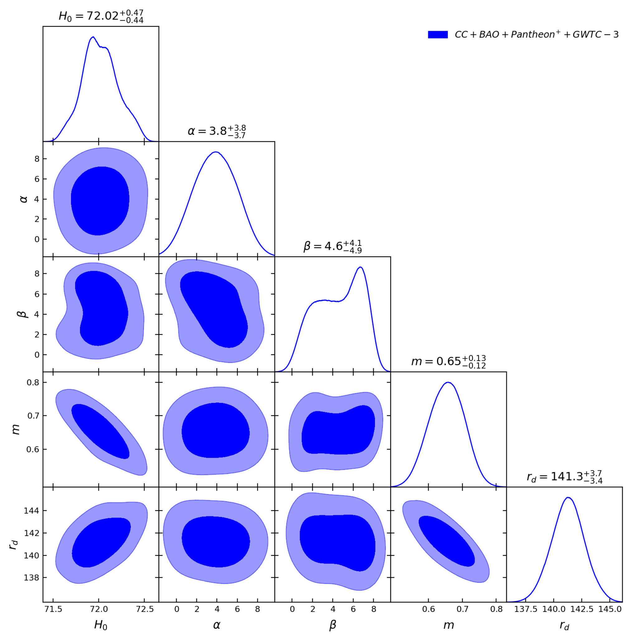
Using Equation (68), we performed the data analysis for the data sets as explained in Section 3. The parameters we want to constrain are $(H_0,\beta ,m,r_d)$. Figure 1 shows the best-fit values for the parameters of this model. The best-fit values of these model parameters are shown in

Table 1. Best fit parameter values for Model I from MCMC.

Datasets	${\mathit{H}}_0\left(\mathbf{km}/\mathbf{s}/\mathbf{Mpc}\right)$	$\mathit{\beta }$	m	${\mathit{r}}_{\mathit{d}}\left(\mathbf{Mpc}\right)$	${\mathit{\chi }}_{\mathbf{min}}^2$	${\mathit{\chi }}_{\mathbf{min}}^2$/dof	p-Value
Priors	(60, 80)	(−4, 4)	(0, 1)	(100, 200)
$CC$	$68.1_{-6.5}^{+7.8}$	$0.6_{-4.3}^{+4.6}$	$0.{54}_{-0.34}^{+0.41}$	${150}_{-50}^{+50}$	$14.692$	$0.509$	$0.99$
$CC+BAO$	$68.6_{-5.3}^{+4.9}$	$0.{46}_{-4.0}^{+3.6}$	$0.{52}_{-0.22}^{+0.24}$	${147}_{-8.5}^{+9.9}$	$7.457$	$0.625$	$0.96$
$CC+BAO+Pantheo{n}^{+}$	$73.{22}_{-0.52}^{+0.53}$	$2.4_{-3.7}^{+2.2}$	$0.{55}_{-0.15}^{+0.15}$	$136.2_{-3.1}^{+3.3}$	$1762.251$	$1.029$	$0.19$
$CC+BAO+Pantheo{n}^{+}+GW$	$72.{62}_{-0.49}^{+0.49}$	$-0.7_{-3.4}^{+4.3}$	$0.{40}_{-0.12}^{+0.16}$	$140.0_{-3.0}^{+3.3}$	$2109.809$	$2.199$	$9.04\times {10}^{-161}$

for different data sets and the joint analysis together with the priors. Interestingly, we see that the joint analysis of $CC+BAO+Pantheo{n}^{+}$ and $CC+BAO+Pantheo{n}^{+}+GW$ gives the present value of the Hubble parameter as $73.{22}_{-0.52}^{+0.53}$ and $72.{62}_{-0.49}^{+0.49}$, respectively, as in par with the direct measurement of the 2019 SH0ES collaboration ($H_0=(74.03\pm 1.42)$ km/s/MPc) [46]. Thus, this model clearly alleviates the existing tension related to the present value of the Hubble parameter without the need for any cosmological constant. The corresponding best fit values of ($\beta ,m,r_d$) are ($2.4_{-3.7}^{+2.2},0.{55}_{-0.15}^{+0.15},136.2_{-3.1}^{+3.3}$) and ($-0.7_{-3.4}^{+4.3},0.{40}_{-0.12}^{+0.16},140.0_{-3.0}^{+3.3}$) respectively. 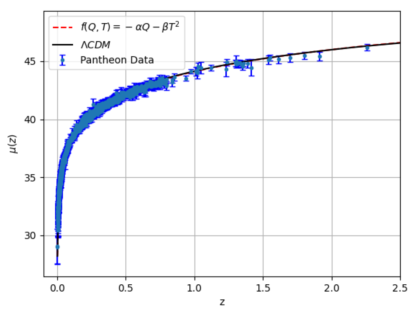In Figure 2 we have plotted our model and $\mathrm{\Lambda }CDM$ model with the best-fit model parameters along with the $Pantheo{n}^{+}$ data, with their error bars. As we can see, our model fits the data as good as $\mathrm{\Lambda }$CDM.

Other Cosmological Behaviors:

In order to further investigate the cosmological behavior of the model, we begin by examining the evolution of the Hubble parameter with respect to redshift z in the context of the $\mathrm{\Lambda }$CDM model. It is well known that the Hubble parameter in $\mathrm{\Lambda }$CDM cosmology is given by:

$$H_{\mathrm{\Lambda }CDM}\left(z\right)=H_0\sqrt{{\mathrm{\Omega }}_{m_0}{(1+z)}^3+1-{\mathrm{\Omega }}_{m_0}}$$

(69)

where $H_0$ is the present day value of the Hubble parameter and ${\mathrm{\Omega }}_{m_0}$ is the present value of density parameter of matter defined as ${\mathrm{\Omega }}_{m_0}={\displaystyle \frac{{\rho }_{m0}}{3H_0^2}}$ in Planck units. We set $H_0=67.8$ km/s/Mpc and ${\mathrm{\Omega }}_{m0}=0.3089$ according to [47].

Now, defining the density parameter for our model, $\mathrm{\Omega }={\displaystyle \frac{8\pi G\rho }{3H^2}}$ for which we have,

$$\mathrm{\Omega }\left(z\right)={\displaystyle \frac{48\pi \alpha H^2}{3H^2[\beta (\omega -3)-16\pi ]}}$$

(70)

By using Equation (68) for the best-fit parameter values shown in Figure 1 and comparing $\mathrm{\Omega }(z=0)$ to 0.3089, Planck result [47] stated above, we found that for $\alpha =-0.317$ and $G=1$, from the above equation, we will get the matter density parameter as ${\mathrm{\Omega }}_m\left(z\right)=0.3086{(1+z)}^3$.

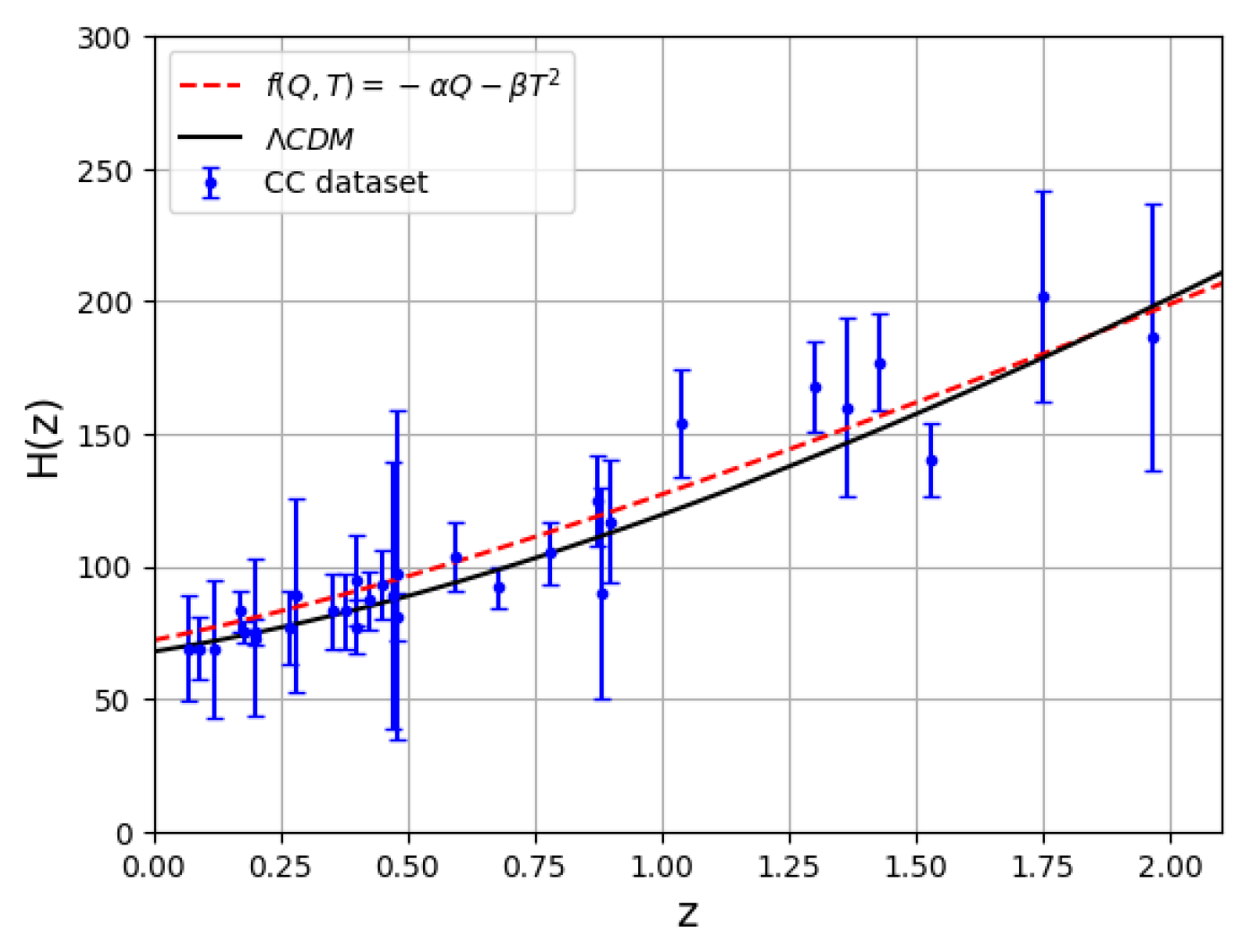
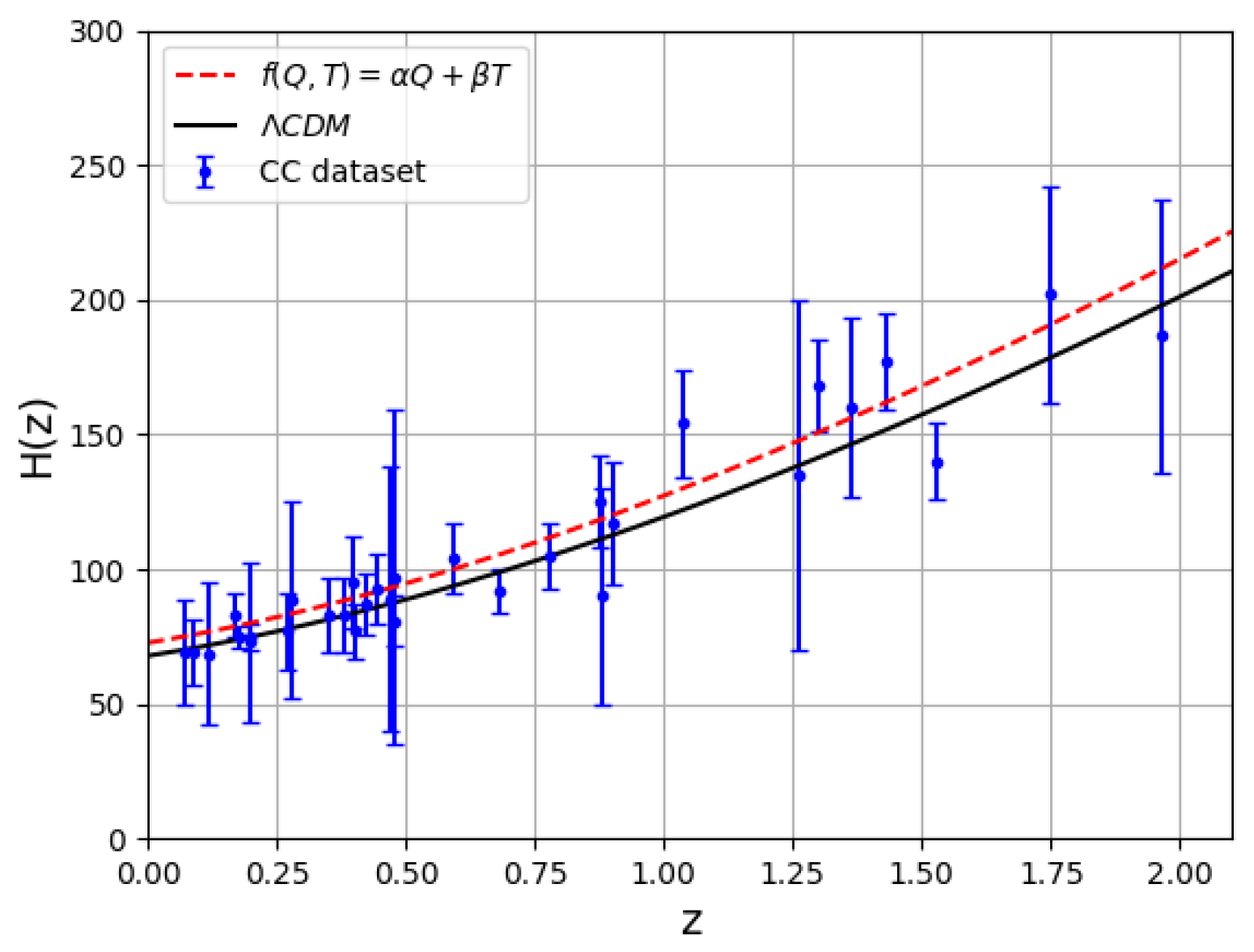
In Figure 3 we present the evolution of the Hubble parameter given by Equation (68) with respect to redshift z along with the CC data set. Here we have plotted the behavior of $H\left(z\right)$ as obtained from Model I by using the best-fit parameter values as shown in Figure 1 along with the $\mathrm{\Lambda }CDM$ model and the observed data accompanied by error bars. The consistency between the model predictions and the observational data is clearly illustrated by the overlapping error bars. This visual agreement supports the reliability of our model in accurately reproducing the behavior of the Hubble function.

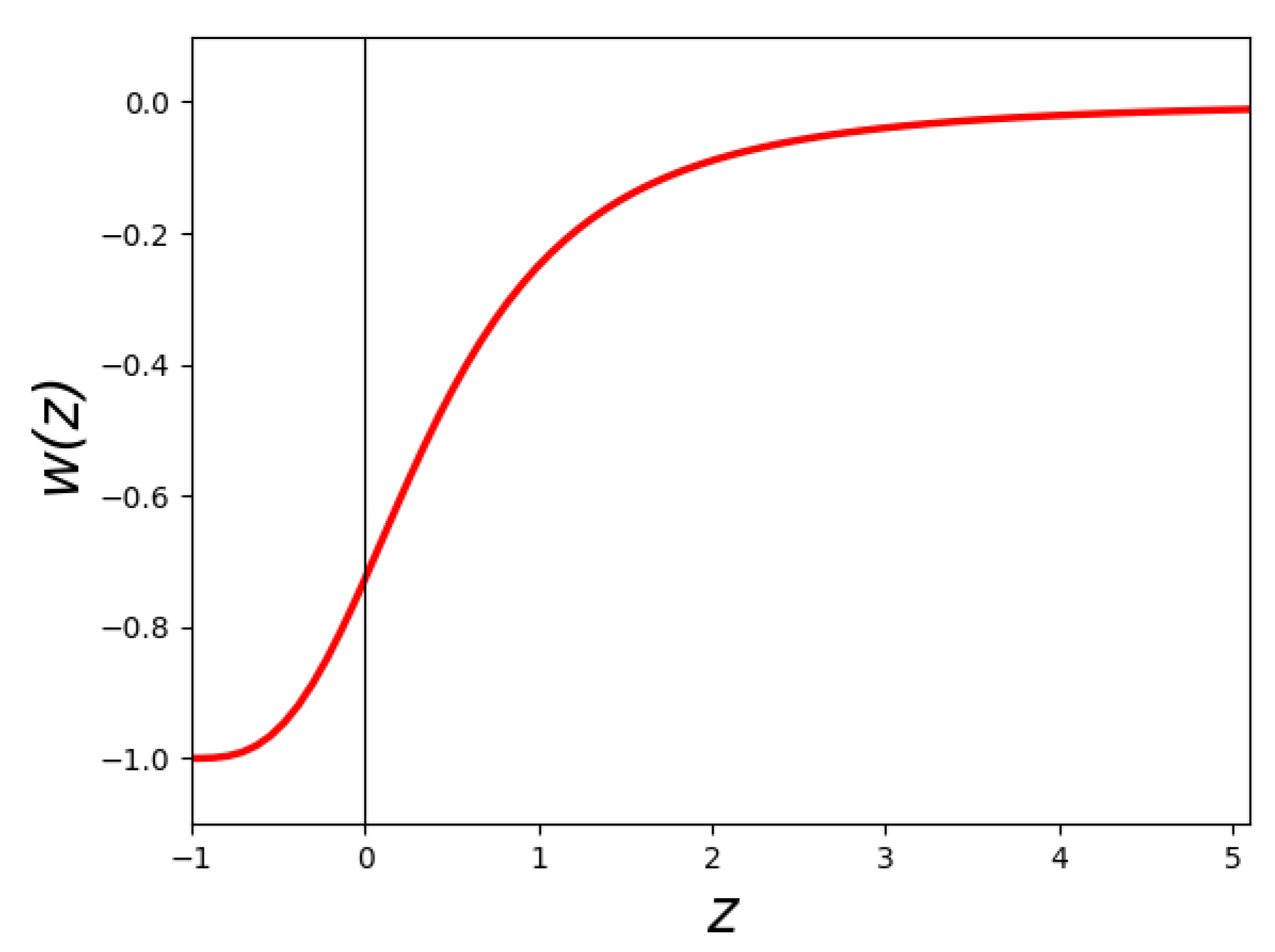
The equation of state (EoS) parameter $\omega$, characterizes the relationship between the pressure and energy density of the cosmic fluid, given by $\omega ={\displaystyle \frac{p}{\rho }}$. Distinct cosmological epochs are associated with specific values of $\omega$: for $\omega =0$, the Universe is in the dust-dominated (matter-dominated) phase; for $\omega ={\displaystyle \frac{1}{3}}$, it is in the radiation-dominated phase; and for $\omega =-1$, it corresponds to vacuum energy, consistent with the $\mathrm{\Lambda }$CDM model. Recent discussions in cosmology emphasize the accelerating expansion of the Universe, which occurs when $\omega <-{\displaystyle \frac{1}{3}}$. This accelerating regime includes the quintessence phase ($-1<\omega <0$) and the phantom phase ($\omega <-1$).

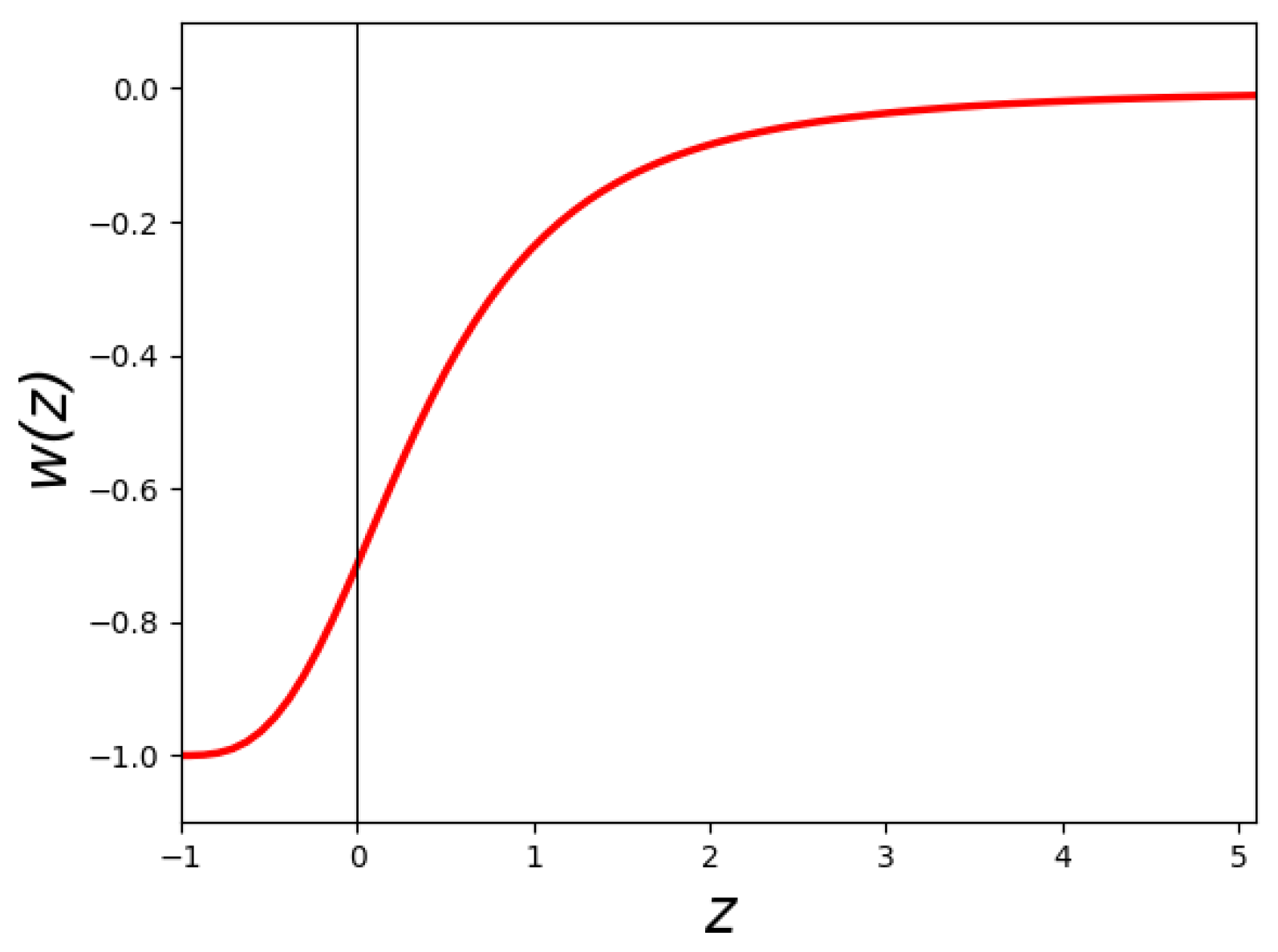
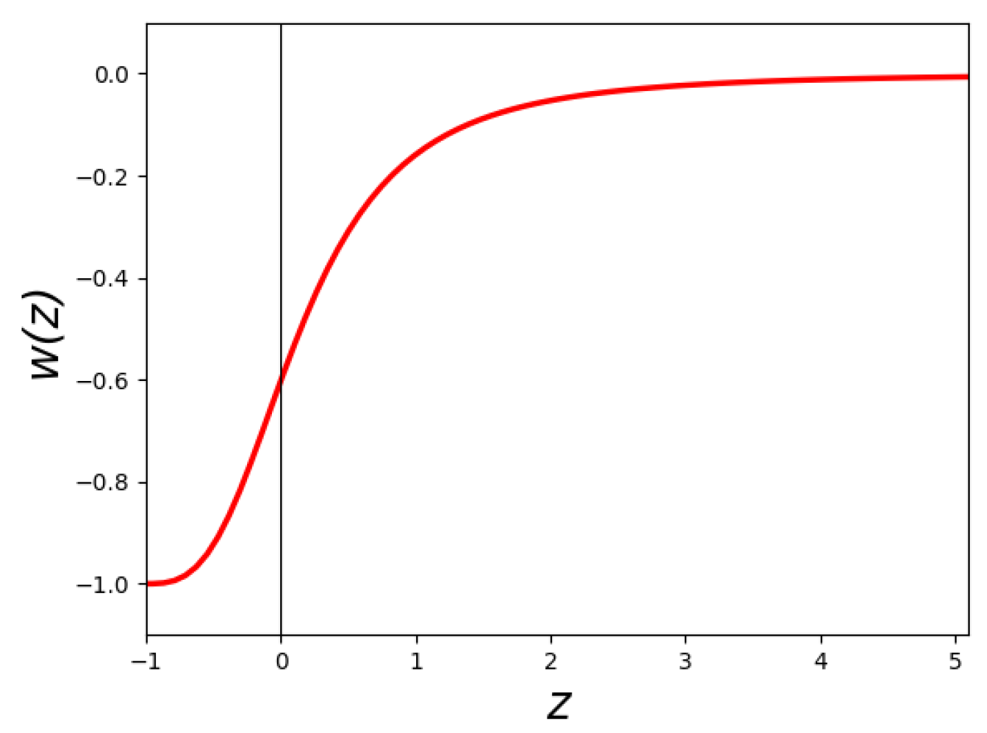
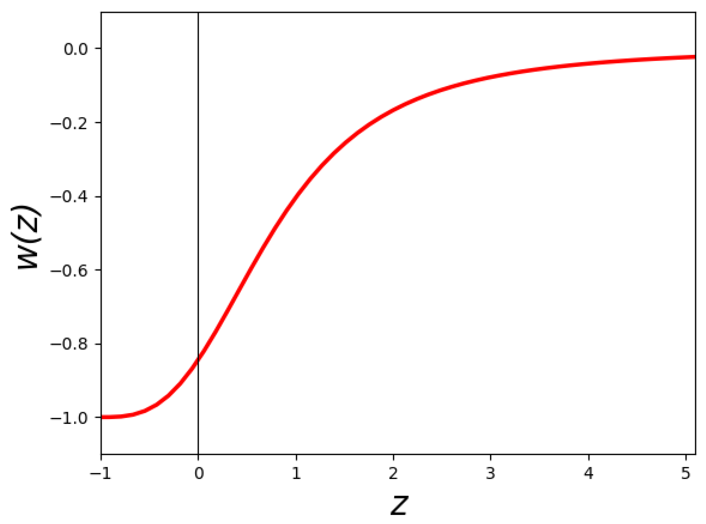
In Figure 4 we have shown the behavior of the Eos parameter for the best-fit parameter value of m as obtained for Model I. The value of Eos parameter at $z=0$ is ${\omega }_0=-0.{72}_{-0.05}^{+0.08}$ which indicates an accelerating phase. Future behavior indicates the Eos tending towards the value $-1$. As we move to higher redshifts, the Eos approaches to $\omega =0$ which represents the dust phase.

Now, the deceleration parameter as a function of Hubble parameter H is defined as,

$$q=-1-{\displaystyle \frac{\dot{H}}{H^2}}$$

(71)

The above equation can be written w.r.t. redshift as:

$$q=-1+(1+z){\displaystyle \frac{1}{H\left(z\right)}}{\displaystyle \frac{dH}{dz}}$$

(72)

In cosmological models, the deceleration parameter q plays a pivotal role in characterizing the dynamics of the Universe’s expansion. It helps determine whether the Universe is undergoing decelerated expansion ($q>0$) or accelerated expansion ($q<0$). For Model I, the deceleration parameter(q) is given by the expression:

$$q=-1+{\displaystyle \frac{3m(8\pi +\beta ){(1+z)}^3}{[\beta +(16\pi +3\beta )(1+m{(1+z)}^3)]}}$$

(73)

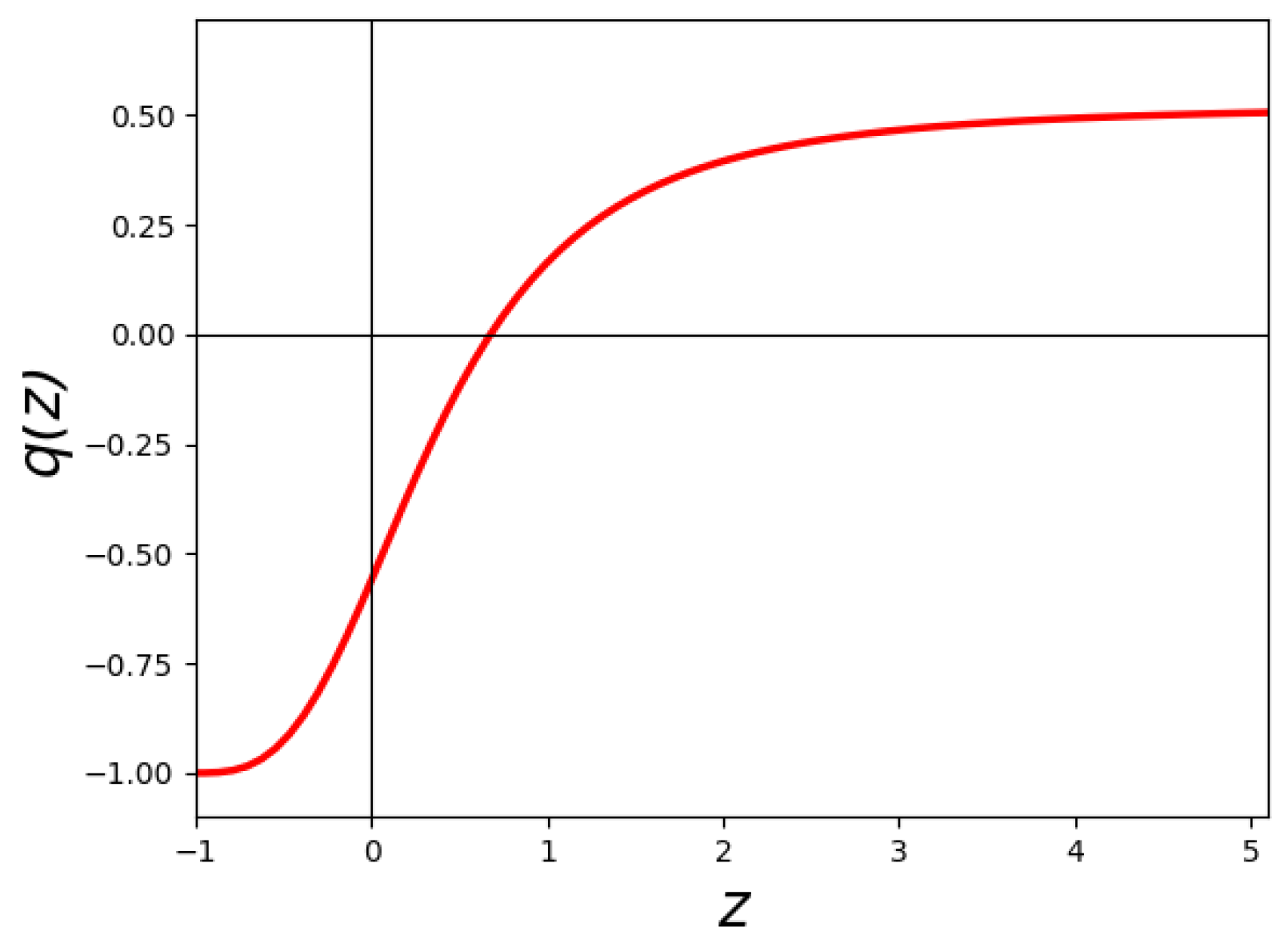
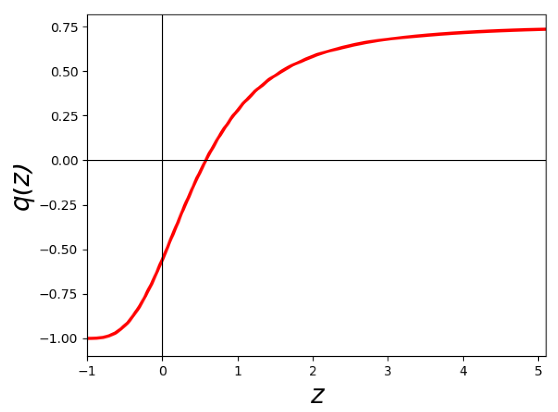
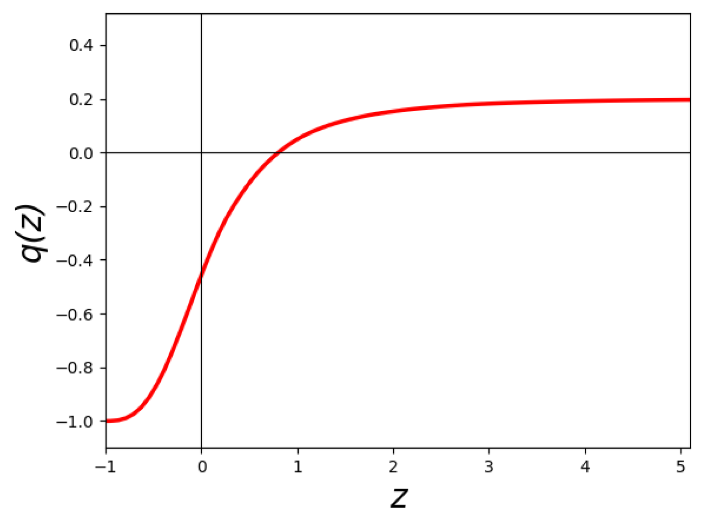
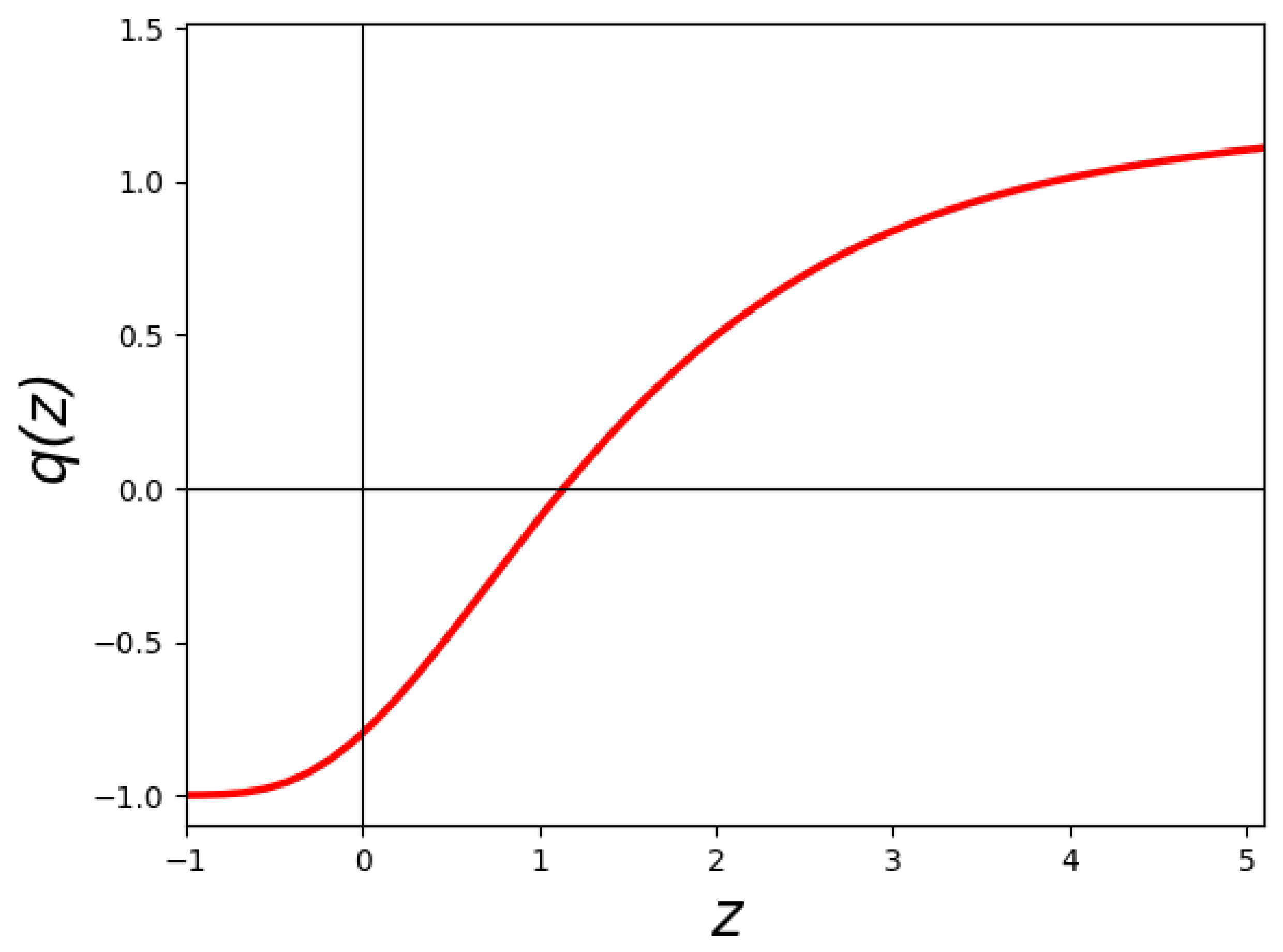
The evolution of the deceleration parameter $q\left(z\right)$ is depicted in Figure 5, based on the best-fit values of the model parameters $\beta$ and m obtained through the MCMC analysis. The plot clearly demonstrates a smooth and consistent transition from a decelerated expansion phase to the current accelerated phase of the Universe.

Also, we have found out that the present day value of the deceleration parameter is, $q_0=-0.{54}_{-0.03}^{+0.04}$ which is negative at present time that represents the accelerating phase of the universe. The deceleration parameter tends towards $-1$ as we go to future redshifts.

Gravitational wave analysis:

The modified GW luminosity distance Equation (37) in Gpc unit, for Model I, takes the form,

$$d_L^{gw}=c(1+z){\int }_0^z{\displaystyle \frac{d{z}^{\prime }}{H\left(z^{\prime }\right)}}\times {10}^{-3}$$

(74)

As we can see, there is no deviation of $d_L^{gw}$ from $d_L^{em}$, which was expected in the presence of linear dependence on Q. For an explicit evaluation of the gravitational wave (GW) luminosity distance, it is essential to compute the Hubble parameter $H\left(z\right)$, which has been obtained in Equation (68) by solving the Friedmann equations given in Equations (16) and (17). Furthermore, to numerically estimate the deviation from the standard $\mathrm{\Lambda }$CDM cosmology, we employ the best-fit results from a joint MCMC analysis using four observational datasets: cosmic chronometers (CC), baryon acoustic oscillations (BAO), the Pantheon⁺ compilation, and the GWTC-3 catalog of gravitational wave events.

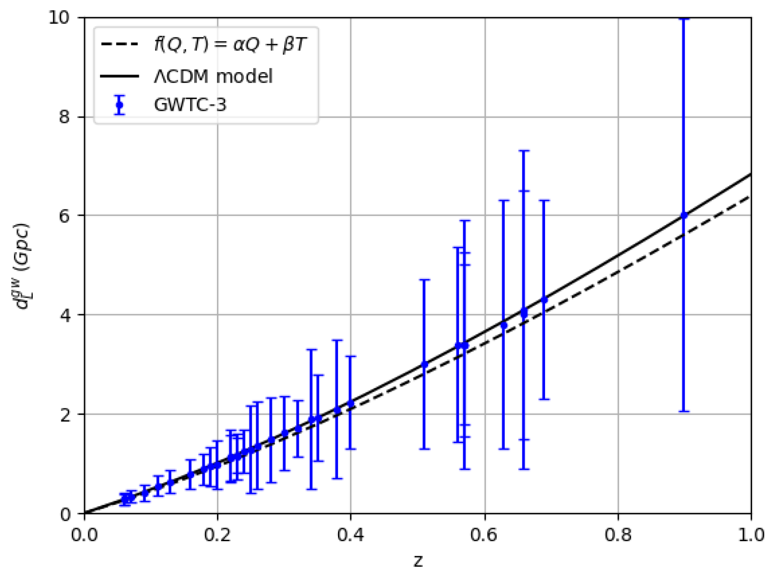
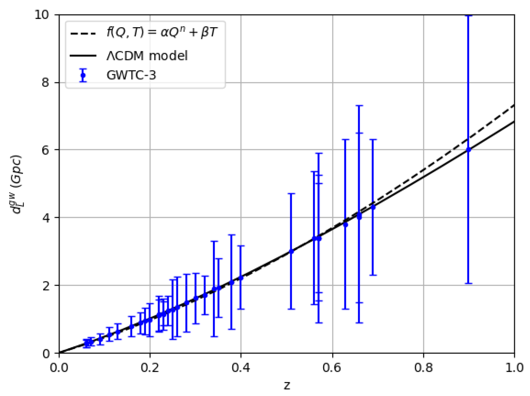
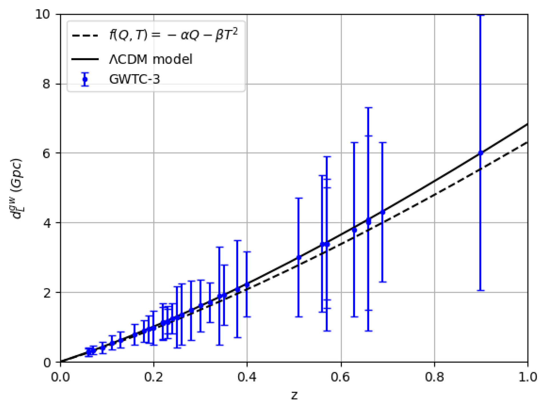
In Figure 6, we have shown the GW luminosity distance along with the $\mathrm{\Lambda }CDM$ model and the observational data. The figure shows a very good agreement of our model with the $\mathrm{\Lambda }CDM$ model and LIGO-VIRGO GW data.

Energy conditions:

The energy conditions are defined as [48]:

1.

Null Energy Condition (NEC): $\rho +p\ge 0$

2.

Weak Energy Condition (WEC): $\rho \ge 0$ and $\rho +p\ge 0$

3.

Strong Energy Condition (SEC): $\rho +p\ge 0$ and $\rho +3p\ge 0$

4.

Dominant Energy Condition (DEC): $\rho \pm p\ge 0$

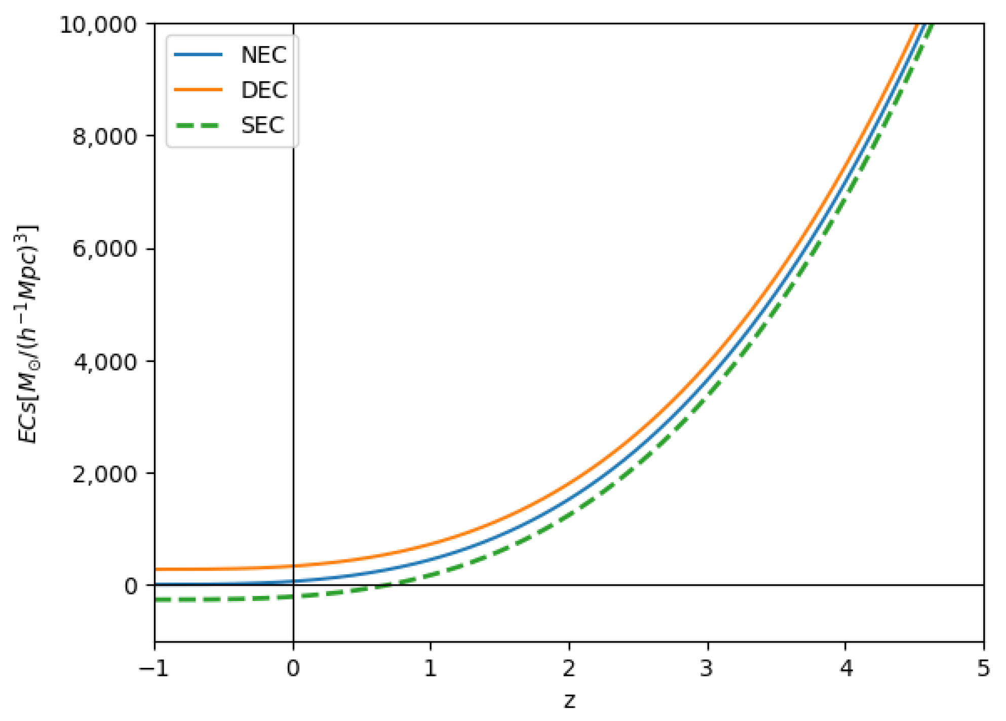
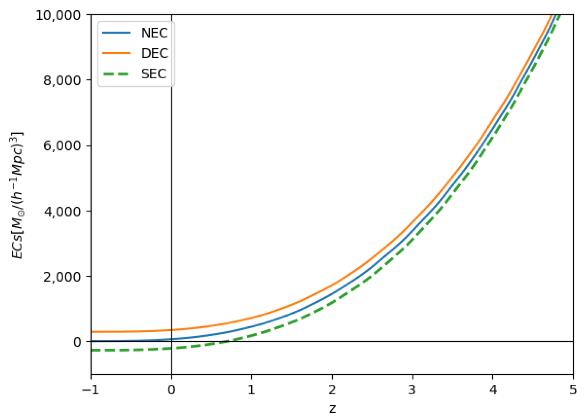
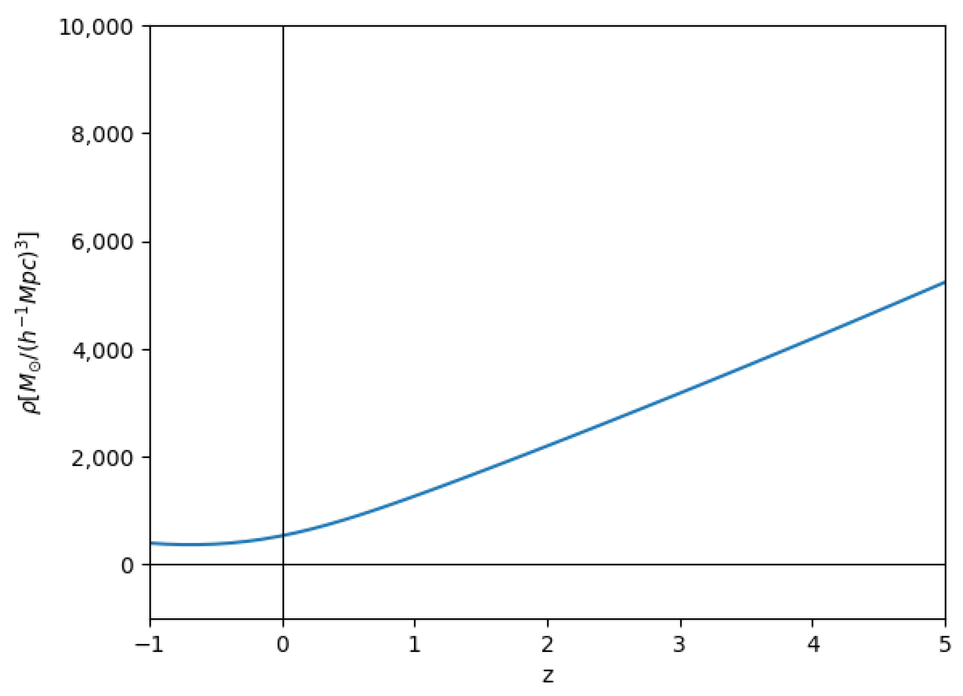
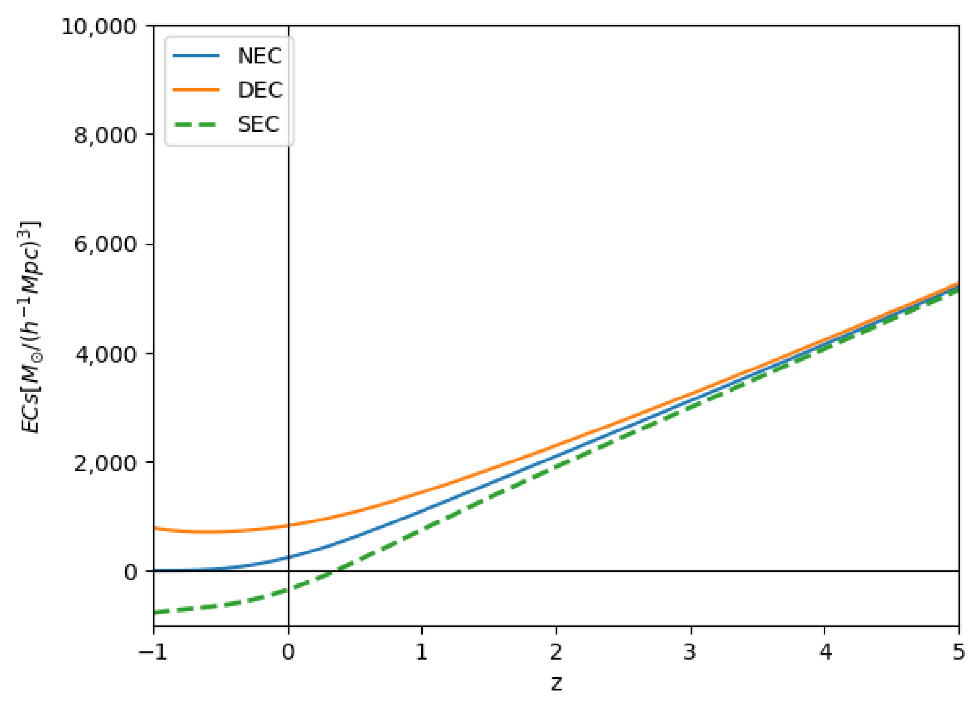
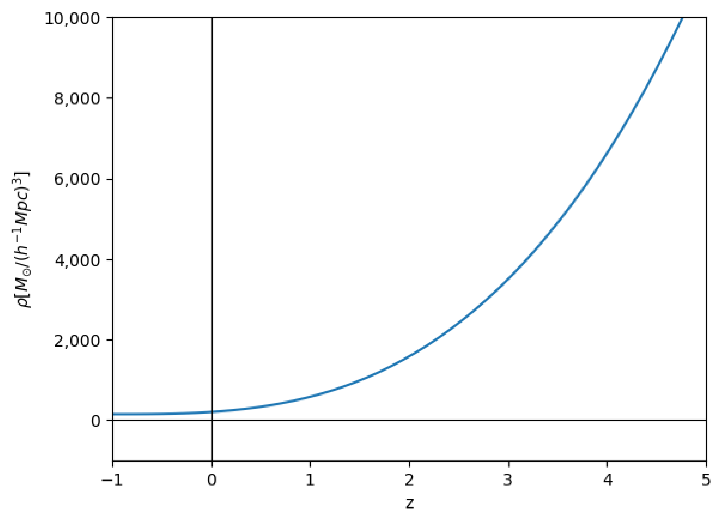
Among the various energy conditions, the strong energy condition (SEC) has the significant attention. Recent observational data indicating the accelerated expansion of the Universe necessitate a violation of the SEC on cosmological scales. As evident from Figure 7, our best-fit model parameters yield a negative value for the SEC at the present epoch, confirming its violation. In contrast, both the null energy condition (NEC) and the dominant energy condition (DEC) remain satisfied. 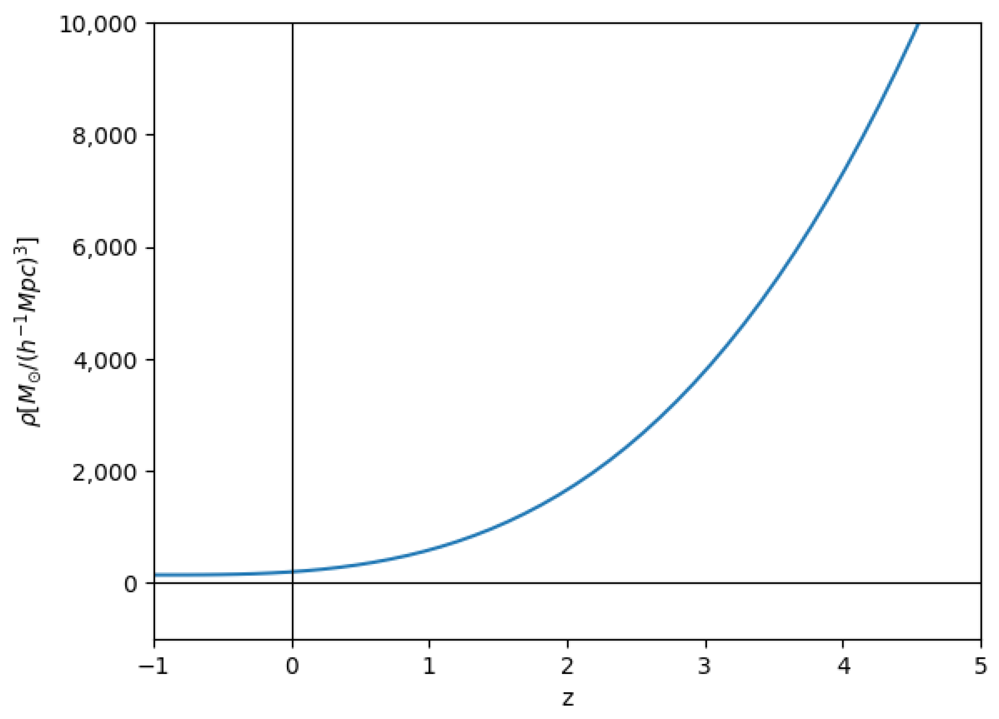Additionally, the behavior of the energy density, as depicted in Figure 8, supports this conclusion. Since the NEC being a component of the weak energy condition (WEC) is satisfied alongside a positive energy density, we conclude that the WEC is also upheld by our model. It is crucial to emphasize that the preceding analysis is restricted entirely to the background cosmological evolution. While our selected $f(Q,T)$ models exhibit phenomenologically viable background behaviors and satisfy the standard weak, null, and dominant energy conditions (with the necessary violation of the strong energy condition to allow for late-time cosmic acceleration), this does not inherently guarantee the complete physical viability of the models. Specifically, our background analysis makes no claims regarding the perturbative stability of these functional forms. As has been recently documented in the broader $f\left(Q\right)$ gravity literature, such non-metric extensions can frequently suffer from pathological ghost instabilities or strong-coupling problems in the scalar and vector perturbation sectors [49]. A comprehensive perturbative analysis, which is beyond the scope of this current phenomenological background study, would be required to definitively confirm the theoretical stability and absence of ghosts in these specific $f(Q,T)$ parameterizations.

4.2. Model II: f(Q,T) $=\alpha Q^n+\beta T$

For the second example, we consider a general ‘n’ dependence on Q. Our model takes the form, $f(Q,T)=\alpha Q^n+\beta T$, where $\alpha ,\beta$ are constants [16]. Here,

$$F=f_Q=n\alpha Q^{n-1}=n\alpha 6^{n-1}{H}^{2n-2};8\pi \tilde{G}=f_T=\beta$$

(75)

From Equation (20) the expression for energy density can be written as,

$$\rho ={\displaystyle \frac{\alpha 6^n{H}^{2n}(1-2n)}{16\pi +(3-\omega )\beta }}$$

(76)

Since, Equation (76) will be negative for the discussed range of free parameters of this model, we must take the value of the adjustable free parameter $\alpha$, so that $\rho$ takes positive values.

Similar to the earlier cases, from the Friedmann Equations (16) and (17) for this particular form, we obtain the form of $\omega$ as,

$$\omega ={\displaystyle \frac{(16\pi +3\beta )\dot{H}+\frac{3}{n}(8\pi +\beta )H^2}{\beta \dot{H}-\frac{3}{n}(8\pi +\beta )H^2}}$$

(77)

By using Equations (22) and (62) we obtain the differential equation for the Hubble parameter as,

$${\displaystyle \frac{dH}{dz}}={\displaystyle \frac{3m(8\pi +\beta ){(1+z)}^{2}H\left(z\right)}{n[\beta +(16\pi +3\beta )(1+m{(1+z)}^3)]}}$$

(78)

Finally, solving the equation we obtain the Hubble parameter as,

$$H\left(z\right)=H_0{\left({\displaystyle \frac{\beta +(16\pi +3\beta )(1+m{(1+z)}^3)}{\beta +(16\pi +3\beta )(1+m)}}\right)}^l$$

(79)

where $l={\displaystyle \frac{(8\pi +\beta )}{n(16\pi +3\beta )}}$ and $H_0$ is Hubble parameter value at present day, i.e., at $z=0$.

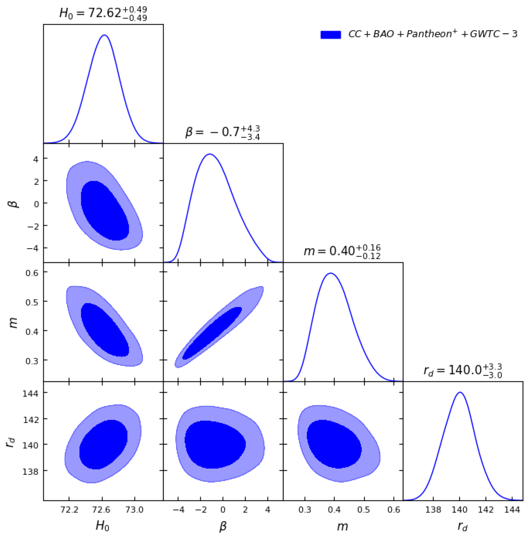
Figure 9 contour plot shows the best-fit values for the parameters of this model. The best-fit values of the model parameters are shown in

Table 2. Best fit parameter values for Model II from MCMC.

Datasets	${\mathit{H}}_0\left(\mathbf{km}/\mathbf{s}/\mathbf{Mpc}\right)$	$\mathit{\beta }$	m	n	${\mathit{r}}_{\mathit{d}}\left(\mathbf{Mpc}\right)$	${\mathit{\chi }}_{\mathbf{min}}^2$	${\mathit{\chi }}_{\mathbf{min}}^2$/dof	p-Value
Priors	(60, 80)	(−10, 10)	(0, 1)	(0, 3)	(100, 200)
$CC$	$68.1_{-6}^{+8}$	$-1.2_{-9.1}^{+9.7}$	$0.{58}_{-0.49}^{+0.49}$	$1.{17}_{-0.65}^{+0.89}$	${150}_{-50}^{+50}$	$15.727$	$0.582$	$0.96$
$CC+BAO$	$68.6_{-5.1}^{+5.3}$	$0.2_{-10.1}^{+9.5}$	$0.{47}_{-0.32}^{+0.47}$	$1.{05}_{-0.28}^{+0.47}$	$147.1_{-8.9}^{+10.1}$	$1.842$	$0.517$	$0.99$
$CC+BAO+Pantheo{n}^{+}$	$73.{01}_{-0.62}^{+0.60}$	$-0.4_{-9.2}^{+10.1}$	$0.{56}_{-0.26}^{+0.33}$	$1.{12}_{-0.25}^{+0.44}$	$136.2_{-3.3}^{+3.3}$	$1760.791$	$1.025$	$0.23$
$CC+BAO+Pantheo{n}^{+}+GW$	$72.{64}_{-0.51}^{+0.53}$	$1.0_{-9.7}^{+9.3}$	$0.{40}_{-0.17}^{+0.17}$	$0.{99}_{-0.21}^{+0.34}$	$140.0_{-3.2}^{+3.2}$	$2079.582$	$2.180$	$1.4\times {10}^{-156}$

for the joint analysis of different data sets. In terms of Hubble tension the present value of Hubble parameter is nearly same as what we obtained for Model I. The best-fit value of the model parameters ($\beta ,m,n,r_d$) from the joint analysis of $CC+BAO+Pantheo{n}^{+}+GW$ data are ($1.0_{-9.7}^{+9.3},0.{40}_{-0.17}^{+0.17},0.{99}_{-0.21}^{+0.34},{140}_{-3.2}^{+3.2}$). Similarly to the earlier cases, in Figure 10 we have plotted our model and the $\mathrm{\Lambda }CDM$ model for the best-fit parameter values obtained from MCMC along with the $Pantheo{n}^{+}$ SNe Ia data.

Other Cosmological Behaviors:

Like before we define the density parameter for our model, $\mathrm{\Omega }={\displaystyle \frac{8\pi \rho }{3H^2}}$ for which we have,

$$\mathrm{\Omega }\left(z\right)={\displaystyle \frac{8\pi \alpha 6^n{H}^{2n}(1-2n)}{3H^2[16\pi +(3-\omega )\beta ]}}$$

(80)

$$\begin{array}{c}\hfill \mathrm{\Omega }\left(z\right)={\displaystyle \frac{8\pi \alpha }{3H^2\left[\left(\frac{(16\pi +\beta )}{2}\right)\left(\frac{(16\pi +3\beta )}{2}\right)-\left(\frac{3\beta }{2}\right)\left(\frac{\beta }{2}\right)\right]}}\times \\ \hfill [{\displaystyle \frac{(16\pi +3\beta )}{2}}\left(6^n{H}^{2n}({\displaystyle \frac{1}{2}}-n)-{\displaystyle \frac{2\beta (2n-1)}{(8\pi +\beta )}}n{6}^{n-1}{H}^{2n-2}\dot{H}\right)\\ \hfill +{\displaystyle \frac{3\beta }{2}}\left(6^n{H}^{2n}(n-{\displaystyle \frac{1}{2}})+2(2n-1)n{6}^{n-1}{H}^{2n-2}\dot{H}\right)]\end{array}$$

(81)

By putting the Equation (79) for the best fit parameter values shown in Figure 9 and comparing $\mathrm{\Omega }(z=0)$ to 0.3089, Planck result [47] stated above, we found that for $\alpha =-0.375$, from the above equation, we will get the matter density parameter as ${\mathrm{\Omega }}_m\left(z\right)=0.3089{(1+z)}^3$.

In Figure 11 we present the evolution of the Hubble function Equation (79) with respect to redshift z by using the best-fit parameter value shown in Figure 9 along with the $\mathrm{\Lambda }CDM$ model and the observed data in $H\left(z\right)$. The agreement between the model prediction and observed data is corroborated from the consistency of the error bars for lower redshifts, but shows slight disagreement for higher redshifts.

Similarly to Model I, we have shown the behavior of the Eos parameter in Figure 12 for the best-fit parameter value of m. The value of Eos parameter at present day($z=0$) is ${\omega }_0=-0.{74}_{-0.05}^{+0.03}$ which indicates an accelerating phase of the universe.

The equation of deceleration parameter q takes the following form for ModelII,

$$q=-1+{\displaystyle \frac{3m(8\pi +\beta ){(1+z)}^3}{n[\beta +(16\pi +3\beta )(1+m{(1+z)}^3)]}}$$

(82)

The behavior of deceleration parameter is shown in Figure 13 for the best fit parameter values of $\beta ,m$ and n. We found that there is a well-behaved transition from deceleration to the acceleration phase, and the present day value of q is $q_0=-0.{57}_{-0.01}^{+0.04}$ indicating the accelerating phase of the universe.

Gravitational wave analysis:

For the present case, the modified GW luminosity distance in Gpc unit takes the form,

$$d_L^{gw}=c(1+z){\left({\displaystyle \frac{H\left(0\right)}{H\left(z\right)}}\right)}^{n-1}{\int }_0^z{\displaystyle \frac{d{z}^{\prime }}{H\left(z^{\prime }\right)}}\times {10}^{-3}$$

(83)

where $H\left(z\right)$ is given by the Equation (79) and $H\left(0\right)$ is the present day value of Hubble parameter given by this model. Using a similar technique, we applied the results of the MCMC joint analysis of the four data sets for this model.

In Figure 14, we have shown the modified GW luminosity distance along with the $\mathrm{\Lambda }CDM$ model and the observational data. The figure shows an excellent match of our model with the $\mathrm{\Lambda }CDM$ model.

Energy conditions:

In Figure 15 and Figure 16, we have shown the nature of energy density and energy conditions. From these figures, it is evident that the violation of SEC at present epoch and satisfaction of the other energy conditions.

4.3. Model III: f(Q,T) $=-\alpha Q-\beta T^2$

As a third example of cosmological model in $f(Q,T)$ gravity, we have considered the case having non-linear dependence on T. We considered the following form, $f(Q,T)=-\alpha Q-\beta T^2$, where $\alpha$ and $\beta$ are positive constants [16]. For this model we have,

$$F=f_Q=-\alpha$$

(84)

$$8\pi \tilde{G}=f_T=-2\beta T=2\beta (1-3\omega )\rho$$

(85)

From Equation (20), the cosmological density will be,

$$\rho ={\displaystyle \frac{6\alpha H^2-\beta {(3\omega -1)}^2{\rho }^2}{16\pi [1+(1+\omega )\tilde{G}]}}$$

(86)

which has the physical solution,

$$\rho ={\displaystyle \frac{8\pi \left[\sqrt{1+3\alpha \beta (1-3\omega )(\omega +5)H^2/32{\pi }^2}-1\right]}{\beta (1-3\omega )(\omega +5)}}$$

(87)

Now, the evolution equation of Hubble parameter for this model takes the form,

$$\begin{array}{c}\dot{H}=-{\displaystyle \frac{32{\pi }^2(1+\omega )}{\alpha \beta (1-3\omega )(\omega +5)}}\times \hfill \\ \hspace{1em}\hspace{1em}\hspace{1em}\hspace{1em}\hspace{1em}\hspace{1em}\hspace{1em} \left[\sqrt{1+3\alpha \beta (1-3\omega )(\omega +5)H^2/32{\pi }^2}-1\right]\times \hfill \\ \hspace{1em}\hspace{1em}\hspace{1em}\hspace{1em}\hspace{1em}\hspace{1em}\hspace{1em} \left[1-{\displaystyle \frac{2\beta (3\omega -1)\left(\sqrt{1+3\alpha \beta H^2(1-3\omega )(\omega +5)/32{\pi }^2}-1\right)}{\beta (1-3\omega )(\omega +5)}}\right]\hfill \end{array}$$

(88)

The corresponding evolution of Hubble parameter with respect to redshift z will be,

$$\begin{array}{c}(1+z)H\left(z\right){\displaystyle \frac{dH}{dz}}={\displaystyle \frac{3(1+\omega )}{\delta }}\left(\sqrt{1+\delta H^2}-1\right)\times \hspace{1em}\hspace{1em}\hspace{1em}\hspace{1em}\hspace{1em}\hspace{1em}\hspace{1em}\hspace{1em}\hspace{1em}\hspace{1em}\hspace{1em}\hspace{1em}\hspace{1em}\hfill \\ \hfill \left(1-{\displaystyle \frac{2\beta (3\omega -1)\left(\sqrt{1+\delta H^2}-1\right)}{\beta (1-3\omega )(\omega +5)}}\right)\end{array}$$

(89)

where,

$$\delta ={\displaystyle \frac{3\alpha \beta (1-3\omega )(\omega +5)}{32{\pi }^2}}$$

(90)

and $\omega$ is given by the Equation (62). The parameters that will be constrained by the data for the present case are ($H_0,\alpha ,\beta ,m,r_d$).

In Figure 17, the contour plot shows the the best-fit values for the parameters of this model. The best-fit value of the model parameters are shown in

Table 3. Best fit parameter values for Model III from MCMC.

Datasets	${\mathit{H}}_0\left(\mathbf{km}/\mathbf{s}/\mathbf{Mpc}\right)$	$\mathit{\alpha }$	$\mathit{\beta }$	m	${\mathit{r}}_{\mathit{d}}\left(\mathbf{Mpc}\right)$	${\mathit{\chi }}_{\mathbf{min}}^2$	${\mathit{\chi }}_{\mathbf{min}}^2$/dof	p-Value
Priors	(60, 80)	(0, 8)	(0, 8)	(0, 2)	(100, 200)
$CC$	$67.2_{-5.0}^{+6.9}$	$3.9_{-4}^{+3.9}$	$4_{-4.1}^{+3.9}$	$0.{77}_{-0.36}^{+0.28}$	${149}_{-50}^{+50}$	$15.468$	$0.573$	$0.96$
$CC+BAO$	$66.3_{-4.1}^{+4.8}$	$2.9_{-3.1}^{+5.7}$	$2.{74}_{-3.5}^{+5.1}$	$0.{90}_{-0.28}^{+0.11}$	$147.8_{-9.1}^{+9.8}$	$4.729$	$0.594$	$0.97$
$CC+BAO+Pantheo{n}^{+}$	$72.{65}_{-0.51}^{+0.52}$	$4.4_{-3.8}^{+4.9}$	$5.3_{-6.2}^{+4.4}$	$0.{73}_{-0.19}^{+0.55}$	$139.5_{-4.2}^{+4.1}$	$1749.581$	$1.020$	$0.28$
$CC+BAO+Pantheo{n}^{+}+GW$	$72.{02}_{-0.44}^{+0.47}$	$3.8_{-3.7}^{+3.8}$	$4.6_{-4.9}^{+4.1}$	$0.{65}_{-0.12}^{+0.13}$	$141.3_{-3.4}^{+3.7}$	$2111.735$	$2.193$	$2.24\times {10}^{-159}$

for different datasets and the joint analysis with the priors. As we can see, joint analysis of $CC+BAO+Pantheo{n}^{+}$ gives the present value of $H_0$ as $72.{65}_{-0.51}^{+0.52}$ km/s/Mpc, thus nearly alleviating the Hubble tension. The corresponding best fit values of the model parameters ($\alpha ,\beta ,m,r_d$) are ($4.4_{-3.8}^{+4.9},5.3_{-6.2}^{+4.4},0.{73}_{-0.19}^{+0.55},139.5_{-4.2}^{+4.1}$). Joint analysis with the GW data, reduces the present value of $H_0$ to $72.{02}_{-0.44}^{+0.47}$ km/s/Mpc, which is still a large improvement over $\mathrm{\Lambda }CDM$, thus reducing the tension with SHOES data. The corresponding best fit values of the model parameters ($\alpha ,\beta ,m,r_d$) are ($3.8_{-3.7}^{+3.8},4.6_{-4.9}^{+4.1},0.{65}_{-0.12}^{+0.13},141.3_{-3.4}^{+3.7}$). In Figure 18 our model with the best parameter values obtained from joint analysis of $CC+BAO+Pantheo{n}^{+}+GW$ and the $\mathrm{\Lambda }CDM$ model has been plotted along with $Pantheo{n}^{+}$ SNe Ia findings for comparison. Like for the other cases, our model fits the data as well as the $\mathrm{\Lambda }$CDM.

Other Cosmological Behaviors:

Now, defining the density parameter for our model, $\mathrm{\Omega }={\displaystyle \frac{8\pi \rho }{3H^2}}$ and putting Equation (87), for which we have,

$$\mathrm{\Omega }\left(z\right)={\displaystyle \frac{{\left(8\pi \right)}^2\left[\sqrt{1+3\alpha \beta (1-3\omega )(\omega +5)H^2/32{\pi }^2}-1\right]}{3H^2\beta (1-3\omega )(\omega +5)}}$$

(91)

By using the solution of Equation (89) and for the best fit parameter values, the matter density parameter will be, ${\mathrm{\Omega }}_m=0.851{(1+z)}^3$ and for the present day value it gives ${\mathrm{\Omega }}_{m0}=0.851$. The value obtained from the density parameter of matter is significantly higher than the value predicted by the standard $\mathrm{\Lambda }CDM$ model (≈0.3). This suggests that the model may overestimate the matter content of the universe, potentially impacting the expansion history and structure formation.

In Figure 19 we present the evolution of the Hubble function by solving Equation (89) with respect to the redshift z by using the best-fit parameter value shown in Figure 17 along with the $\mathrm{\Lambda }CDM$ model and the observed data on $H\left(z\right)$, associated with the error bars. Model III agrees nearly as well with the observed data as $\mathrm{\Lambda }$CDM.

Now, we have solved this model numerically and shown the behavior of the Eos parameter in Figure 20 for the best-fit parameter value m. The value of Eos parameter at present day($z=0$) is ${\omega }_0=-0.{63}_{-0.05}^{+0.04}$ indicating, as for the other cases, an accelerating phase of the universe.

The behavior of the deceleration parameter is given by the equation,

$$q=-1+(1+z){\displaystyle \frac{1}{H\left(z\right)}}{\displaystyle \frac{dH}{dz}}$$

(92)

By using Equation (89) and it’s solution we have shown the behavior in Figure 21 for the best fit parameter values of $\alpha$, $\beta$ and m. The present day value of q turns out to be $q_0=-0.{45}_{-0.03}^{+0.05}$.

Gravitational wave analysis:

For the present case, the modified GW luminosity distance in Gpc unit takes the form,

$$d_L^{gw}=c(1+z){\int }_0^z{\displaystyle \frac{d{z}^{\prime }}{H\left(z^{\prime }\right)}}\times {10}^{-3}$$

(93)

where $H\left(z\right)$ is given by the solution of Equation (89) and $H\left(0\right)$ is the present day value of Hubble parameter given by this model. Similarly to the approach used in Model I, we applied the results from the MCMC joint analysis of the four datasets to this model.

In Figure 22, we have plotted the modified GW luminosity distance along with the $\mathrm{\Lambda }CDM$ model and the observational data. The figure shows a very good match of our model with LIGO-VIRGO data.

Energy conditions:

In Figure 23 and Figure 24, we have shown the plot for energy density and energy conditions vs. redshift. From these figures, it is evident that the violation of SEC at present epoch and satisfaction of the other energy conditions.

4.4. Model IV: f(Q,T) $=\alpha Q^{-2}{T}^2$

For our fourth example of cosmological model in $f(Q,T)$ gravity, we will consider a pure non-minimally coupled case which has the form $f(Q,T)=\alpha Q^{-2}{T}^2$. Here, $\alpha$ is a constant. Then we can calculate,

$$F=f_Q=-(\alpha /108H^6){(3\omega -1)}^2{\rho }^2$$

(94)

$$8\pi \tilde{G}=(\alpha /18H^4)(3\omega -1)\rho$$

(95)

From Equation (20), the cosmological density will be,

$$\rho ={\displaystyle \frac{-16\pi H^4}{\alpha [(1/9)(1+\omega )(3\omega -1)-(5/36){(3\omega -1)}^2]}}$$

(96)

Now, the evolution of Hubble parameter for this model takes the form,

$$\dot{H}=-{\displaystyle \frac{18(1+\omega )\left[8\pi +(1/18H^4)(3\omega -1)\rho \right]H^6}{\alpha {(3\omega -1)}^2\rho }}$$

(97)

The evolution of Hubble parameter with respect to redshift z will be,

$${\displaystyle \frac{dH}{dz}}={\displaystyle \frac{18(1+\omega )\left[8\pi +(1/18H^4)(3\omega -1)\rho \right]H^5}{\alpha (1+z){(3\omega -1)}^2\rho }}$$

(98)

The parameters that we will constrain for this case are ($H_0,m,\alpha ,r_d$).

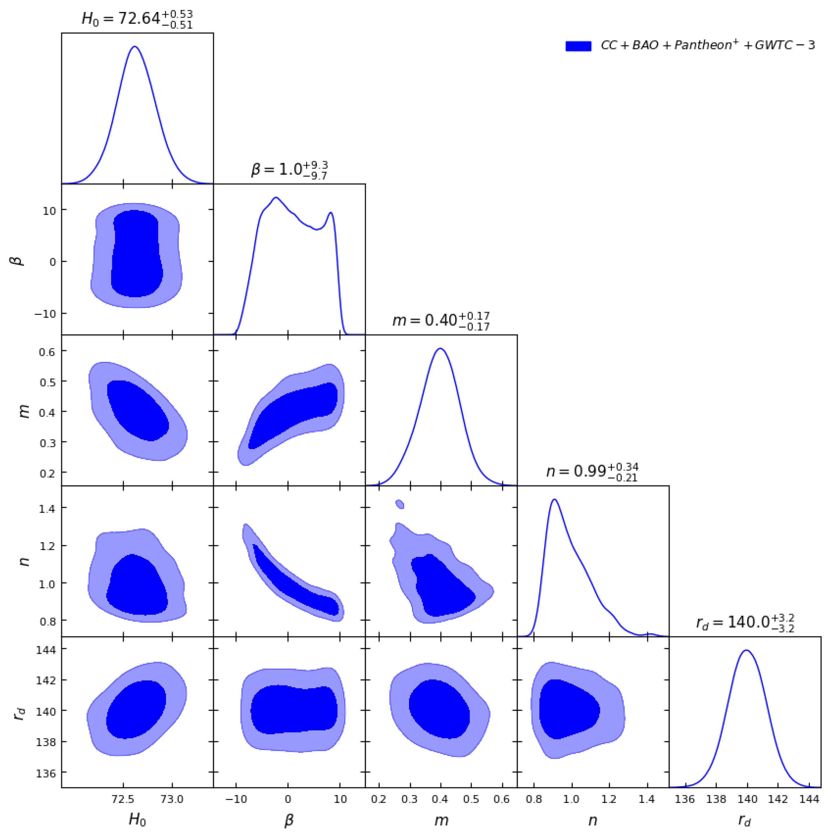
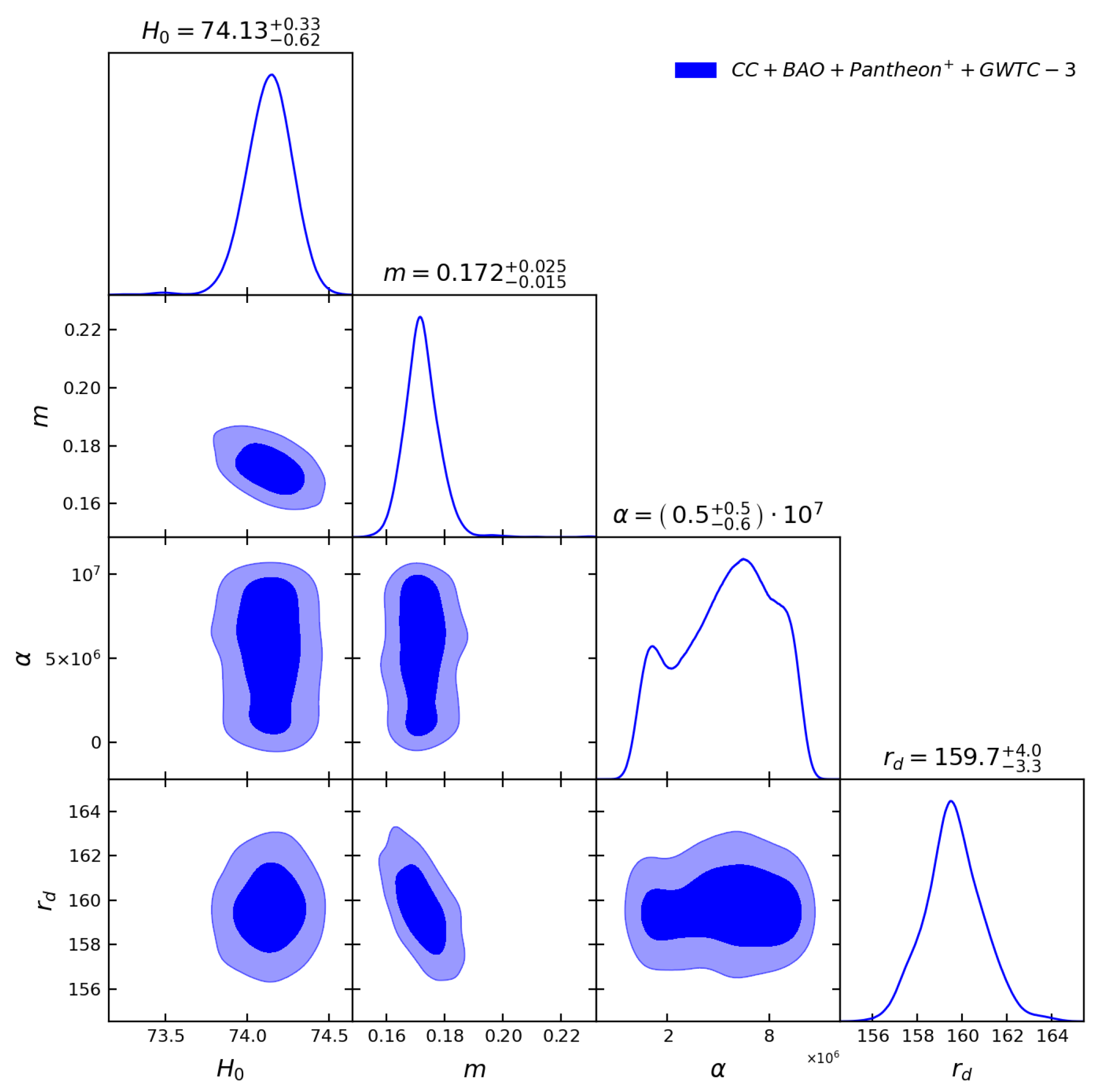
By performing a numerical analysis of the model, we have obtained the best-fit values of the model parameters, as illustrated in the contour plot shown in Figure 25. The corresponding best-fit values for various datasets, as well as their combined joint analysis, are summarized in

Table 4. Best fit parameter values for Model IV from MCMC.

Datasets	${\mathit{H}}_0\left(\mathbf{km}/\mathbf{s}/\mathbf{Mpc}\right)$	m	$\mathit{\alpha }$	${\mathit{r}}_{\mathit{d}}\left(\mathbf{Mpc}\right)$	${\mathit{\chi }}_{\mathbf{min}}^2$	${\mathit{\chi }}_{\mathbf{min}}^2$/dof	p-Value
Priors	(60, 80)	(0, 2)	(0, 10) $\times {10}^6$	(100, 200)
$CC$	${70}_{-6}^{+8}$	$0.{45}_{-0.21}^{+0.40}$	$0.{52}_{-0.51}^{+0.47}\times {10}^7$	${159}_{-50}^{+50}$	$15.572$	$0.555$	$0.97$
$CC+BAO$	$71.8_{-7.3}^{+5.9}$	$0.{33}_{-0.12}^{+0.51}$	$0.{48}_{-0.53}^{+0.51}\times {10}^7$	$149.3_{-20}^{+19}$	$1.198$	$0.478$	$0.99$
$CC+BAO+Pantheo{n}^{+}$	$73.{85}_{-2.3}^{+1.1}$	$0.{43}_{-0.19}^{+0.28}$	$0.{64}_{-0.51}^{+0.39}\times {10}^7$	$140.2_{-11}^{+19}$	$1782.821$	$1.037$	$0.14$
$CC+BAO+Pantheo{n}^{+}+GW$	$74.{13}_{-0.62}^{+0.33}$	$0.{172}_{-0.015}^{+0.025}$	$0.5_{-0.6}^{+0.5}\times {10}^7$	$159.7_{-3.3}^{+4.0}$	$2719.971$	$2.552$	$2.45\times {10}^{-239}$

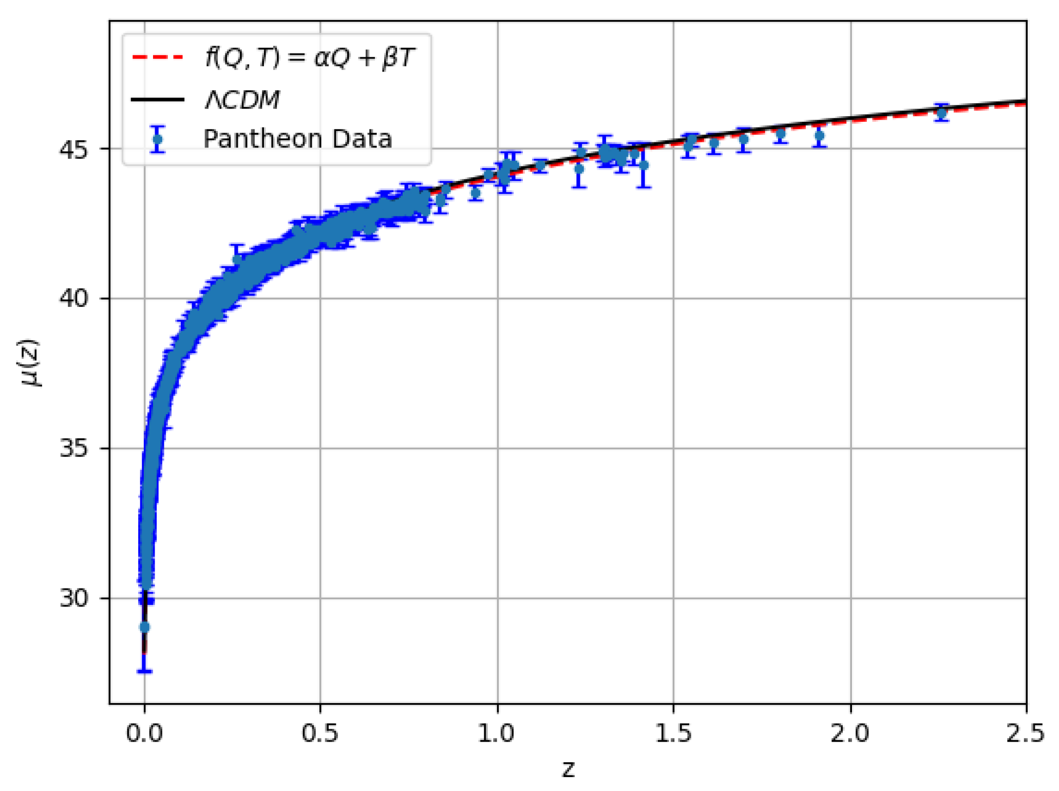
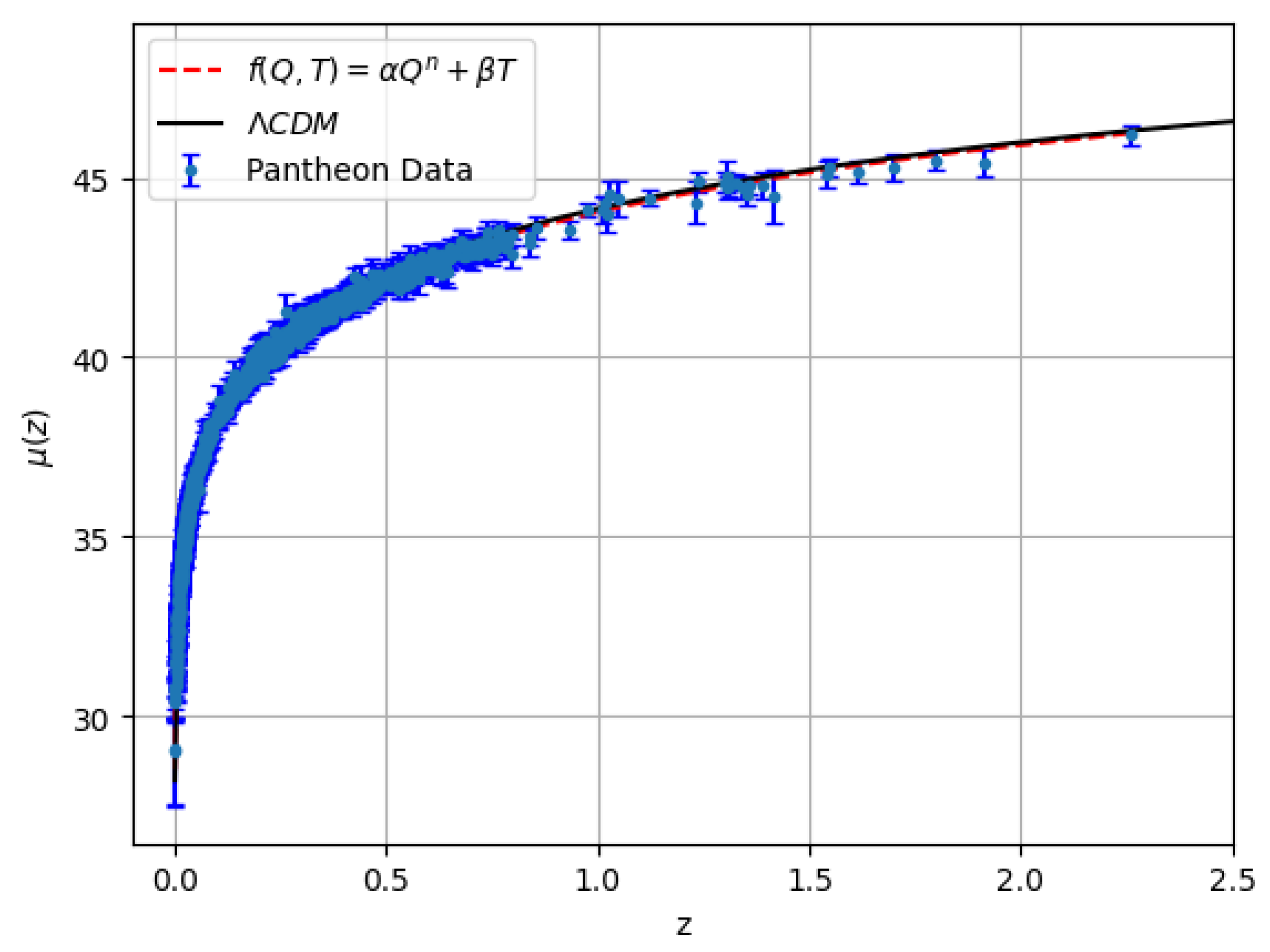
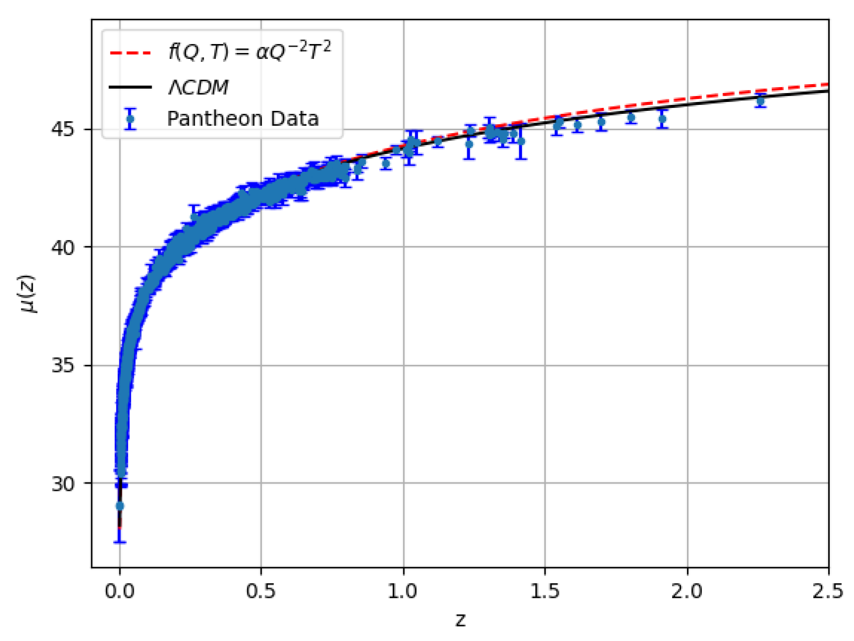
. Our present non-minimally coupled model gives a value of $H_0$ as $74.{13}_{-0.62}^{+0.33}$ km/s/Mpc (from joint analysis of $CC+BAO+Pantheo{n}^{+}+GW$), thus successfully reducing the Hubble tension. In Figure 26, we present the distance modulus evolution for our model alongside the $\mathrm{\Lambda }$CDM model, using the best-fit parameter values obtained from the MCMC analysis. The figure also includes the observational data from the $Pantheo{n}^{+}$ compilation, comprising 1701 SNe Ia data points with associated errors. This allows for a direct visual comparison between the predictions of our model and those of the standard cosmological model.

Other Cosmological Behaviors:

Let us now proceed with the numerical investigation of this model. Similarly to the previous Model III, defining the density parameter for our model, $\mathrm{\Omega }={\displaystyle \frac{8\pi \rho }{3H^2}}$ and putting Equation (96), for which we have,

$$\mathrm{\Omega }\left(z\right)={\displaystyle \frac{-128{\pi }^2{H}^2}{3\alpha [(1/9)(1+\omega )(3\omega -1)-(5/36){(3\omega -1)}^2]}}$$

(99)

By using the solution of Equation (98) and for the best-fit parameter values, the matter density parameter will be, ${\mathrm{\Omega }}_m=0.256{(1+z)}^3$, thus predicting a smaller ${\mathrm{\Omega }}_{m_0}$ as compared to $\mathrm{\Lambda }$CDM.

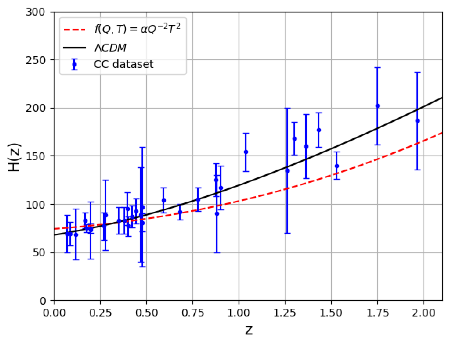
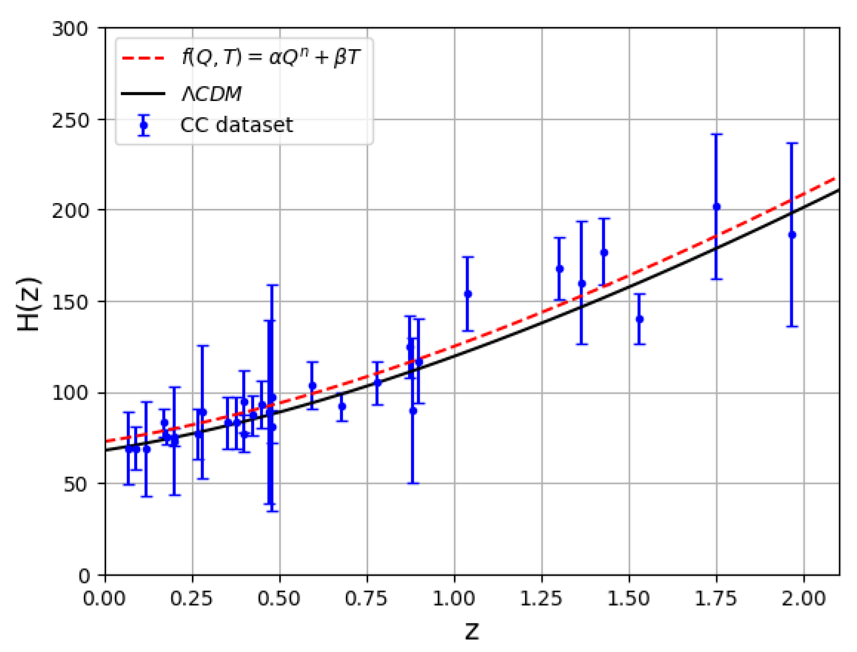
In Figure 27 we present the evolution of the Hubble function by solving Equation (98) with respect to the redshift z by using the best-fit parameter value shown in Figure 25 along with the $\mathrm{\Lambda }CDM$ model and the observed data on $H\left(z\right)$, accompanied by error bars. Our model shows good agreement between the model prediction and observed data for the lower redshift but shows a very poor fit for the higher redshift.

Now, we have solved this model numerically and shown the behavior of the Eos parameter in Figure 28 for the best-fit parameter value m. The value of Eos parameter at present day ($z=0$) is ${\omega }_0=-0.{84}_{-0.02}^{+0.04}$ which indicates an accelerating phase of the universe. The behavior of deceleration parameter,

$$q=-1+(1+z){\displaystyle \frac{1}{H\left(z\right)}}{\displaystyle \frac{dH}{dz}}$$

(100)

By using Equation (98) and it’s solution we have shown in Figure 29 for the best-fit parameter values of $m,\alpha$. We found that there is a well-behaved transition from deceleration to the acceleration phase and the present-day value of q is $q_0=-0.{78}_{-0.06}^{+0.05}$ which is negative at present time, indicating the accelerating phase of the universe.

Gravitational wave analysis:

For this present case, the modified GW luminosity distance in Gpc unit takes the form,

$$d_L^{gw}=c(1+z)\left[{\displaystyle \frac{(3{\omega }_0-1)H{\left(z\right)}^3{\rho }_0}{(3\omega -1)H{\left(0\right)}^3\rho \left(z\right)}}\right]{\int }_0^z{\displaystyle \frac{d{z}^{\prime }}{H\left(z^{\prime }\right)}}\times {10}^{-3}$$

(101)

where $H\left(z\right)$ is given by the solution of Equation (98) and $H\left(0\right)$ is the present day value of Hubble parameter given by this model and $\rho \left(z\right)$ is given by Equation (96) and ${\rho }_0$ represents present value of energy density. Similarly $\omega$ is the Eos parameter given by Equation (62) and ${\omega }_0$ represents its present value for this model. Again, following a similar technique to that of previous models, we have used the result of MCMC of joint analysis of the four datasets for this model.

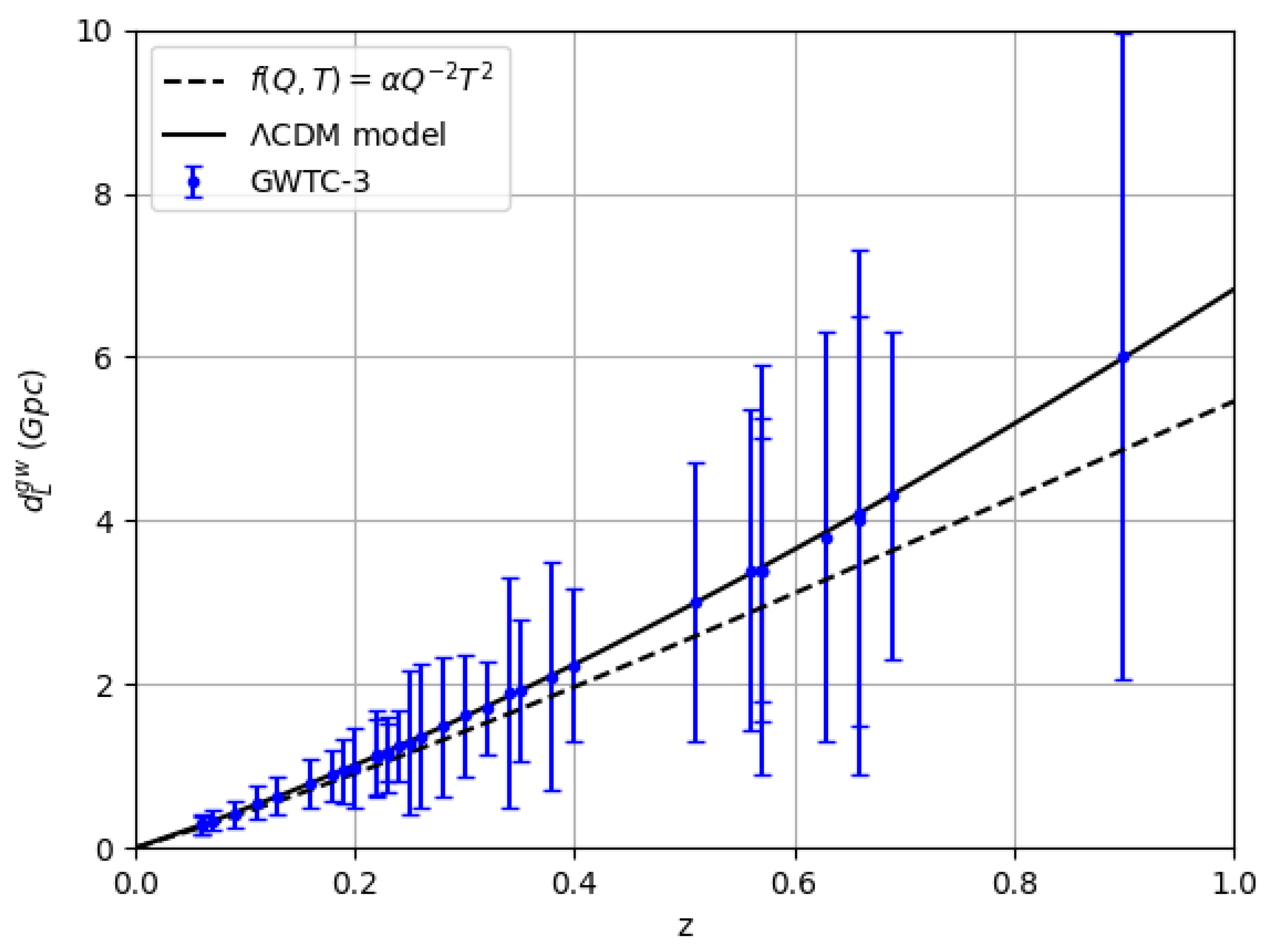
In Figure 30, we have plotted the modified GW luminosity distance along with the $\mathrm{\Lambda }CDM$ model and the observational data. The figure shows the deviation from $\mathrm{\Lambda }CDM$ of our model.

Energy conditions:

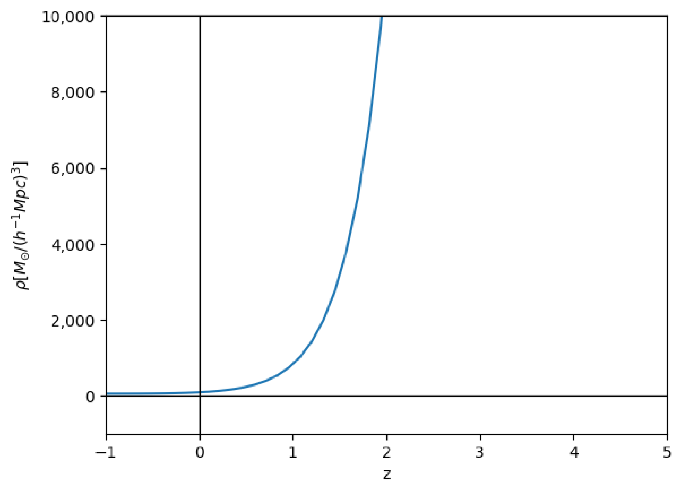
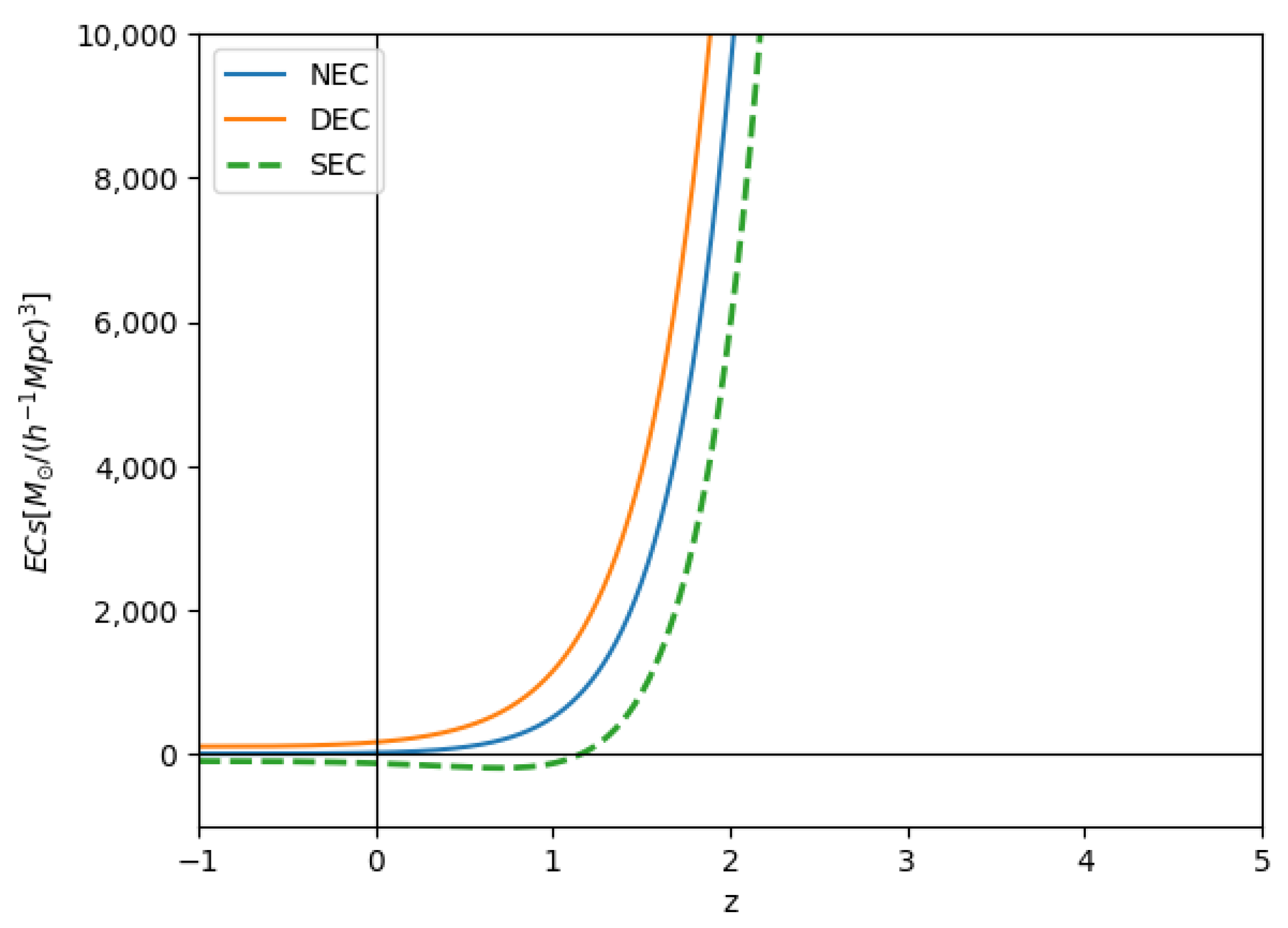
In Figure 31 and Figure 32, we see the nature of energy density and energy conditions. From these figures, it is evident that the violation of SEC at present epoch and satisfaction of the other energy conditions. However the density parameter increases rapidly in and around $z=2$ which is not physical.

5. Model Comparison

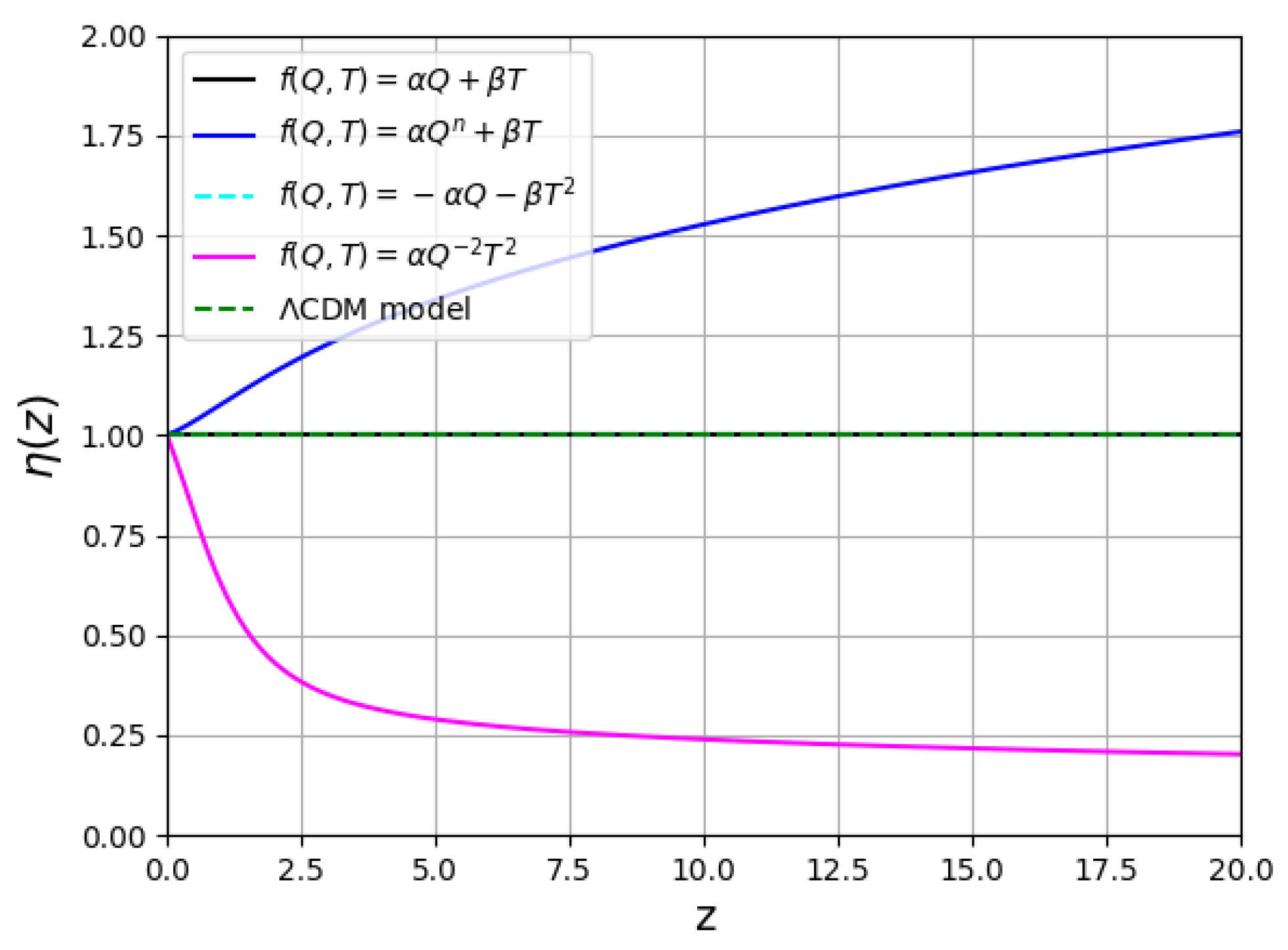
In Figure 33 we have plotted the DDR relation Equation (43) for different $f(Q,T)$ models. We see that there is a deviation in the relation between $d_L^{gw}$ and $d_A$ in the presence of our models $\alpha Q^n+\beta T$ and $\alpha Q^{-2}{T}^2$, while the models $\alpha Q+\beta T$ and $-\alpha Q-\beta T^2$ keep the relationship intact. In this work, the GR curve is represented by the $\mathrm{\Lambda }CDM$ line. A deviation greater than 1, in our case model $\alpha Q^n+\beta T$, means that the observed luminosity distance is larger than predicted by DDR, while the observed angular diameter distance is smaller than predicted. A deviation less than 1, in our case $\alpha Q^{-2}{T}^2$, means that the observed luminosity distance is smaller than predicted by the DDR, while the observed angular diameter distance is larger than predicted. This might have implications on the universe’s expansion (faster/slower than predicted by GR), indicating towards the presence of new physics, which needs to be explored further.

Also we can see, from Equation (35), the ratio $d_L^{gw}/d_L^{em}$ is the same as $\eta \left(z\right)$ in Equation (43) and turn out to be less than 1 for model IV and matches with GR for models I and III, which is also evident from the corresponding expression of $d_L^{gw}$. This implies that, for Model IV, the received gravitational wave (GW) signals appear stronger compared to those predicted by the standard Einstein theory. Consequently, such signals would be more readily detectable for a given source distance and fixed detector sensitivity. Now, the ratio $d_L^{gw}/d_L^{em}$ turns out to be greater than 1 for model II. This implies that the received gravitational wave (GW) signals appear weaker compared to the predictions of standard General Relativity (GR). Consequently, for a fixed source distance and detector sensitivity, such signals would be more challenging to detect.

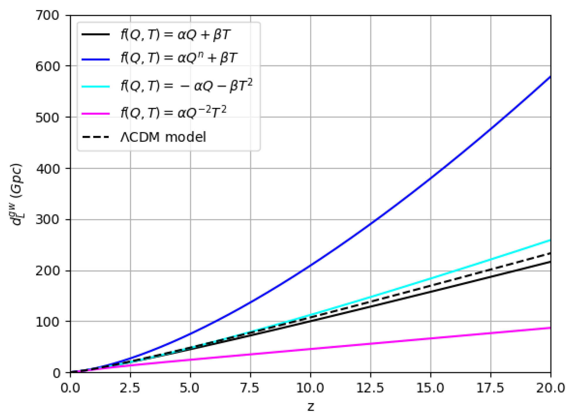
In Figure 34 we have shown the alteration of $d_L^{gw}$ with z for the best-fit parameter values for all the models along with $\mathrm{\Lambda }$CDM for comparison. We can see that though the $d_L^{gw}$ for the models show a similar behavior for small redshifts, their deviations become more prominent as we go to larger z, being maximum for models II and IV.

AIC, BIC & ${\chi }_{min}^2/dof$ values:

In this work, we will use the standard $\mathrm{\Lambda }CDM$ model as the reference model. The MCMC analysis of $\mathrm{\Lambda }CDM$ model is reported in

Table 5. Best fit parameter values for $\mathrm{\Lambda }CDM$ Model from MCMC.

Datasets	${\mathit{H}}_0\left(\mathbf{km}/\mathbf{s}/\mathbf{Mpc}\right)$	${\mathbf{\Omega }}_{{\mathit{m}}_0}$	${\mathit{r}}_{\mathit{d}}\left(\mathbf{Mpc}\right)$	${\mathit{\chi }}_{\mathbf{min}}^2$	${\mathit{\chi }}_{\mathbf{min}}^2$/dof	p-Value
Priors	(60, 80)	(0, 1)	(100, 200)
$CC$	$68.2_{-7}^{+8}$	$0.{331}_{-0.14}^{+0.18}$	$150.9_{-50}^{+50}$	$14.602$	$0.504$	$0.99$
$CC+BAO$	$68.8_{-4.1}^{+4.8}$	$0.{315}_{-0.038}^{+0.049}$	$146.8_{-8.4}^{+8.9}$	$7.493$	$0.614$	$0.97$
$CC+BAO+Pantheo{n}^{+}$	$73.{37}_{-0.47}^{+0.48}$	$0.{316}_{-0.027}^{+0.033}$	$136.5_{-3.1}^{+3.4}$	$1765.372$	$1.029$	$0.19$
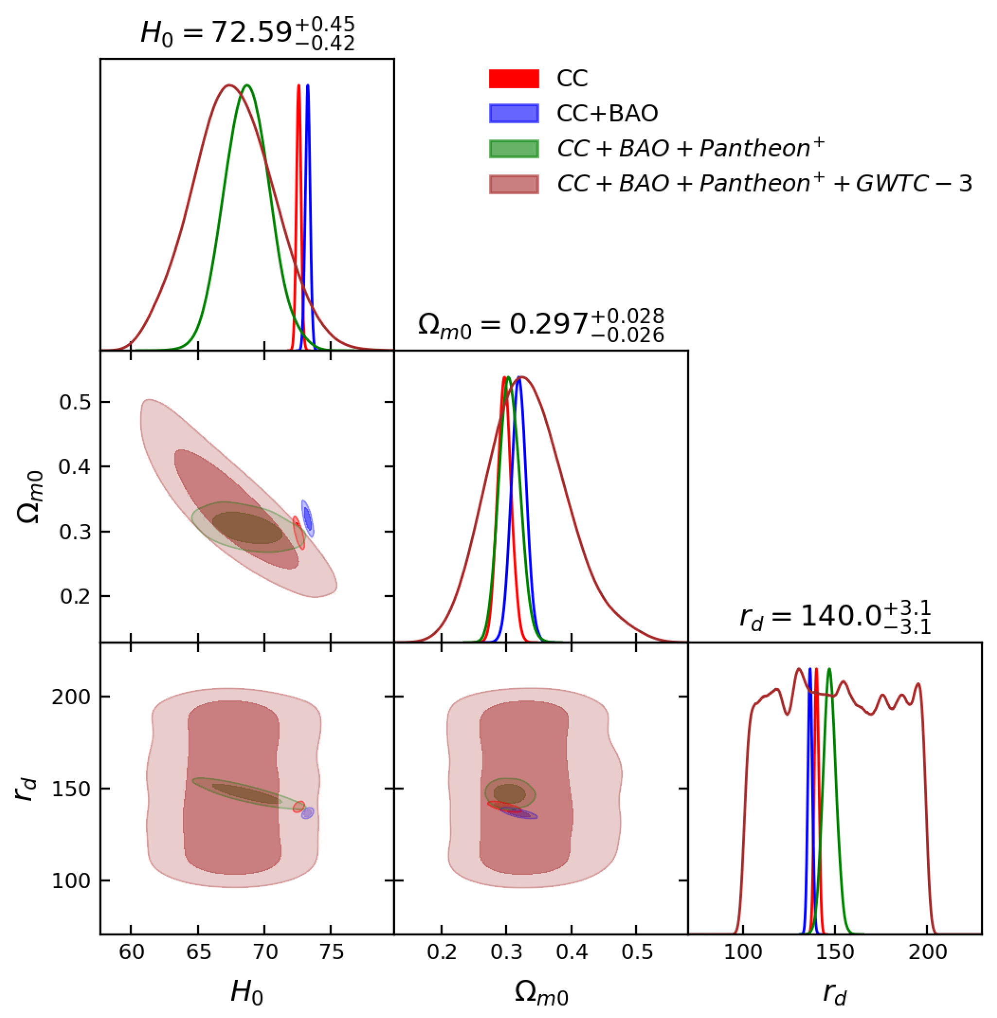
$CC+BAO+Pantheo{n}^{+}+GW$	$72.{59}_{-0.42}^{+0.45}$	$0.{297}_{-0.026}^{+0.028}$	$140.0_{-3.1}^{+3.1}$	$2113.649$	$2.202$	$2.34\times {10}^{-161}$

and contour plot is shown in Figure 35. The AIC and BIC values for all the models and the $\mathrm{\Lambda }CDM$ model are reported in

Table 6. The values for the AIC and BIC criteria for the different models and for the different datasets.

Models	Dataset	AIC	$\mathbf{\Delta }$AIC	BIC	$\mathbf{\Delta }$BIC
$\mathrm{\Lambda }CDM$	$CC$	20.602	0	24.999	0
-	$CC+BAO$	13.493	0	18.484	0
-	$CC+BAO+Pantheo{n}^{+}$	1771.372	0	1787.757	0
-	$CC+BAO+Pantheo{n}^{+}+GW$	2119.649	0	2136.089	0
$\alpha Q+\beta T$	$CC$	22.692	2.09	28.428	3.429
-	$CC+BAO$	15.457	1.964	22.007	3.523
-	$CC+BAO+Pantheo{n}^{+}$	1770.251	−1.121	1792.095	4.338
-	$CC+BAO+Pantheo{n}^{+}+GW$	2117.809	−1.84	2139.726	3.637
$\alpha Q^n+\beta T$	$CC$	25.642	5.04	32.812	7.813
-	$CC+BAO$	10.751	−2.742	18.939	0.455
-	$CC+BAO+Pantheo{n}^{+}$	1772.576	1.204	1799.882	12.125
-	$CC+BAO+Pantheo{n}^{+}+GW$	2092.698	−26.951	2120.095	−15.994
$-\alpha Q-\beta T^2$	$CC$	25.468	4.866	32.638	7.639
-	$CC+BAO$	9.271	−4.222	17.459	−1.025
-	$CC+BAO+Pantheo{n}^{+}$	1759.581	−11.791	1786.886	−0.871
-	$CC+BAO+Pantheo{n}^{+}+GW$	2121.735	2.086	2149.131	13.042
$\alpha Q^{-2}{T}^2$	$CC$	23.527	2.925	29.308	4.309
-	$CC+BAO$	6.802	−6.691	13.352	−11.647
-	$CC+BAO+Pantheo{n}^{+}$	1790.821	19.449	1812.665	24.908
-	$CC+BAO+Pantheo{n}^{+}+GW$	2727.971	608.322	2749.888	613.799

. From Table 6, we can see that model I has good support for the $CC$, $CC+BAO$, $CC+BAO+Pantheo{n}^{+}$ and $CC+BAO+Pantheo{n}^{+}+GW$ datasets according to AIC and BIC criteria, yielding observationally consistent late-time expansion histories, providing strong statistical fits to the combined datasets with ${\chi }_{min}^2/dof$ and p-value indicating reasonable agreement with the data’s noise parameters. In this model, the linear Q parameter $\alpha$ is unconstrained by the MCMC analysis. we have calibrated $\alpha$ post-hoc to align the present-day matter density parameter, ${\mathrm{\Omega }}_{m0}$, with the Planck 2018 results. For $CC+BAO+Pantheo{n}^{+}+GW$ dataset, the model is statistically rejected due to it’s high ${\chi }_{min}^2/dof$ value. For model II, it has no support for the $CC$ data and $CC+BAO+Pantheo{n}^{+}$ specifically for the BIC criteria, but for the $CC+BAO$ data set it is comparable to the reference model. Model II shows very good observational support for the $CC+BAO+Pantheo{n}^{+}+GW$ data from the AIC and BIC criteria. For $CC+BAO+Pantheo{n}^{+}+GW$ dataset, the model is statistically rejected due to it’s high ${\chi }_{min}^2/dof$ value. For model III, we have considered the nonlinear dependence on T, and it shows very good support for the $CC+BAO$, $CC+BAO+Pantheo{n}^{+}$ data sets according to AIC and BIC criteria and reasonable values of ${\chi }_{min}^2/dof$ and p-value, but it does not support for the $CC$ and $CC+BAO+Pantheo{n}^{+}+GW$ dataset. For $CC+BAO+Pantheo{n}^{+}+GW$ dataset, the model is statistically rejected due to it’s high ${\chi }_{min}^2/dof$ value. Model IV involves non-minimally coupling between Q and T and it shows good support for $CC$, $CC+BAO$ data sets but has no support at all for the $CC+BAO+Pantheo{n}^{+}$ and $CC+BAO+Pantheo{n}^{+}+GW$ data sets according to the AIC and BIC criteria. Here also, For $CC+BAO+Pantheo{n}^{+}+GW$ dataset, the model is statistically rejected due to it’s high ${\chi }_{min}^2/dof$ value. It is evident that all models demonstrates observational support for certain datasets or specific combinations of them. However, when evaluated using the AIC and BIC criteria and ${\chi }_{min}^2/dof$ and p-value, all of our models shows statistical disagreement. However, we see that among models I and III, the deceleration parameter for model III takes smaller values for higher redshifts in comparison to $\mathrm{\Lambda }$CDM model. This shows that the transition to the accelerating phase happens faster as compared to the standard model of cosmology. This might have impact on the matter and radiation dominated era, which we will explore in future.

It is important to note that this comparison was made using the $\mathrm{\Lambda }$CDM model as a reference. Using a different reference model or alternative data sets could potentially lead to different conclusions.

6. Conclusions

As new theories of gravity emerge, it is essential to rigorously test their viability in explaining the dark sector of the universe. The $f(Q,T)$ gravity theory, which combines the non-metricity function Q with the trace of the energy-momentum tensor T, presents a promising approach. In this study, we evaluated several viable models of $f(Q,T)$ gravity against both late-time cosmological data and gravitational wave observations to assess their potential.

To begin with, we considered minimally coupled models that have both linear and nonlinear dependence on $Q,T$, having the general form $f(Q,T)=\alpha Q^n+\beta T$. We study the case corresponding to $n=1$.

Model I has the functional form $f(Q,T)=\alpha Q+\beta T$, where $\alpha ,\beta$ are free parameters.

We have used a parametric form of the Eos parameter as a function of redshift z given by Equation (62) to solve the field equations for the Hubble parameter H. This parameter exhibits a negative value during the recent epoch of acceleration. At high redshift z, $\omega$ approaches zero for positive values of the model parameter m, while its value at $z=0$ depends on this parameter. To test our model, we utilized four data sets: the Hubble dataset comprising 32 data points(CC), DESI BAO data set, the $Pantheo{n}^{+}$ dataset with 1701 data points, and the Gravitational Wave data set(GWTC-3). Then we used the MCMC method to put stringent constraints on all the model parameters using the four data sets $(CC,BAO,Pantheo{n}^{+},GWTC-3)$ individually and jointly. The best-fit values of our model parameters from our joint analysis study $(CC+BAO+Pantheo{n}^{+}+GW)$ are as follows: $\beta =-0.7_{-3.4}^{+4.3}$,$m=0.{40}_{-0.12}^{+0.16},r_d=140.0_{-3.0}^{+3.3}$. However, from the $\mathrm{\Lambda }CDM$ model we have obtained the value of $r_d$ as $140.0_{-3.1}^{+3.1}$ for the joint analysis of four data sets. For these best-fit values, our model gives the current value of the Hubble parameter as $H_0=72.{62}_{-0.49}^{+0.49}$ km/s/Mpc. While the joint analysis $(CC+BAO+Pantheo{n}^{+})$ gives a value of $H_0$ as $H_0=73.{22}_{-0.52}^{+0.53}$ km/s/Mpc which is consistent with the latest direct measurement of the Hubble parameter. For these constant values, we have tested our model with GW luminosity distance data points obtained from the $GWTC-3$ catalog (LIGO-VIRGO and KAGRA collaboration) along with the $\mathrm{\Lambda }CDM$ model. Figure 6 shows quite a good match with the observational data points. We then examined the behavior of the Eos parameter and found that the present day value is ${\omega }_0=-0.{72}_{-0.05}^{+0.08}$, which indicates an accelerating phase. Then we also studied the deceleration parameter, and this model predicts the present day value as $q_0=-0.{54}_{-0.03}^{+0.04}$, which is negative at the present time, indicating the accelerating phase of the universe. For this model, the density parameter of matter is given by ${\mathrm{\Omega }}_{m_0}=0.{3086}_{-0.0001}^{+0.0002}$, which is close to the Planck result [47] for $\alpha =-0.{317}_{-0.04}^{+0.07}$.

For our second example, we considered the form $f(Q,T)=\alpha Q^n+\beta T$, where again $\alpha ,\beta ,n$ are free parameters. Similarly to the previous model, we used the same parametric form of equation of state parameter to solve the field equations for H. Then we used the MCMC method to put stringent constraints on the model parameters. The parameters of our study are as follows: $\beta =1.0_{-9.7}^{+9.3}$,$m=0.4_{-0.17}^{+0.17}$,$n=0.{99}_{-0.21}^{+0.34},r_d=140.0.5_{-3.2}^{+3.2}$ obtained from the joint analysis of the 4 data sets. However, from the $\mathrm{\Lambda }CDM$ model we have obtained the value of $r_d$ as $140.0_{-3.1}^{+3.1}$ for the joint analysis of four datasets. For these best-fit values, our model gives the present day value of the Hubble parameter as $H_0=72.{64}_{-0.51}^{+0.53}$ km/s/Mpcs. However, from the joint analysis of $(CC+BAO+Pantheo{n}^{+})$, $H_0=73.{01}_{-0.62}^{+0.60}$ km/s/Mpc which is consistent with the observational data. For these constant values, we have tested our model with GW luminosity distance data points along with the $\mathrm{\Lambda }CDM$ model. Figure 14 shows quite a good match with the observational data points. We then examined the behavior of the Eos parameter and found that the present day value is ${\omega }_0=-0.{74}_{-0.05}^{+0.03}$, which indicates an accelerating phase. Then we also studied the deceleration parameter, and the present day value is $q_0=-0.{57}_{-0.01}^{+0.04}$. For this model, the matter density parameter is given by ${\mathrm{\Omega }}_{m_0}=0.{3089}_{-0.0001}^{+0.0002}$, which is close to the Planck result [47] for $\alpha =-0.{375}_{-10.12}^{+6.27}$.

For our third model, we considered a functional form for a minimally coupled model where we introduced the nonlinearity in T. We considered the given form, $f(Q,T)=-\alpha Q-\beta T^2$, where $\alpha$ and $\beta$ are free, positive parameters. Then we used the MCMC method to constrain the model parameters by using $CC+BAO+Pantheo{n}^{+}+GW$ dataset and we found $\alpha =3.8_{-3.7}^{+3.8}$, $\beta =4.6_{-4.9}^{+4.1}$, $m=0.{65}_{-0.12}^{+0.13},r_d=141.3_{-3.4}^{+3.7}$. For these best-fit parameters, our model gives the Hubble parameter value as $H_0=72.{07}_{-0.44}^{+0.47}$, again showing agreement with the observational data. For these constant values, we have tested our model with GW luminosity distance data points along with the $\mathrm{\Lambda }CDM$ model. Figure 22 shows good agreement with the observational data points. We then examined the behavior of the Eos parameter and found that the present day value is ${\omega }_0=-0.{63}_{-0.05}^{+0.04}$, which indicates an accelerating phase. Then we also studied the deceleration parameter and the present day value is $q_0=-0.{45}_{-0.03}^{+0.05}$, which is negative at present time indicating the accelerating phase of the universe. For this model, the density parameter of matter is given by ${\mathrm{\Omega }}_{m_0}=0.{851}_{-0.23}^{+0.11}$.

For our last model, we considered a particular example of a non-minimally coupled model of the form $f(Q,T)=\alpha Q^{-2}{T}^2$. Using the MCMC method, we found constant values as: $H_0=74.{13}_{-0.62}^{+0.33}$, $m=0.{172}_{-0.015}^{+0.025},\alpha =0.5_{-0.6}^{+0.5}\times {10}^7,r_d=159.4_{-3.3}^{+4.0}$. The larger $r_d$ (compared to the $\mathrm{\Lambda }$CDM) suggests that this $f(Q,T)$ model modifies early-time cosmology, potentially slowing down expansion before recombination. For these constant values, we have tested our model with GW luminosity distance data points along with the $\mathrm{\Lambda }CDM$ model. In Figure 30 we have shown our model with observational data points. We can see the deviation from the $\mathrm{\Lambda }CDM$ model for the higher redshift. We then examined the behavior of the Eos parameter and found that the present day value is ${\omega }_0=-0.{84}_{-0.02}^{+0.04}$, which indicates an accelerating phase. Then we also studied the deceleration parameter and the present day value is $q_0=-0.{78}_{-0.06}^{+0.05}$, which is negative at present time indicating the accelerating phase of the universe. For this model, the density parameter of matter is given by ${\mathrm{\Omega }}_{m_0}=0.{256}_{-0.03}^{+0.06}$.

It is important to highlight the specific role of the parameter $\alpha$ in Models I and II. Because $\alpha$ cancels out of the background Hubble evolution equations, it is unconstrained by our MCMC likelihood analysis. Consequently, we have calibrated $\alpha$ post-hoc to align the present-day matter density parameter, ${\mathrm{\Omega }}_{m0}$, with the Planck 2018 results. However, fixing $\alpha$ in this manner directly alters the effective gravitational coupling, $G_{eff}$. A modified $G_{eff}$ can have significant physical implications, particularly concerning the bounds set by Big Bang Nucleosynthesis (BBN), stringent local gravity tests, and the overall perturbative stability of the model. Therefore, while this calibration ensures a consistent late-time density parameter, the broader physical viability of these specific $\alpha$ values requires future rigorous testing against local and early-universe constraints.

In Section 2 We have investigated the violation of energy conditions (ECs) in the framework of the $f(Q,T)$ gravity model. The primary motivation is to examine the violation of the strong energy condition (SEC) [48], which is often associated with the accelerated expansion of the Universe in the context of modified gravity theories. Utilizing Equations (16) and (17), we have analyzed the behavior of various energy conditions as functions of redshift for our proposed $f(Q,T)$ models. The results show that all four $f(Q,T)$ models under consideration satisfy the weak energy condition (WEC), the null energy condition (NEC), and the dominant energy condition (DEC). However, they exhibit a violation of the SEC, which aligns with the observational evidence of the current accelerated expansion of the Universe.

We further showed that the above models fit quite well with the latest gravitational wave LIGO-VIRGO data($GWTC-3$) based on the study of the modified gravitational wave luminosity distance as discussed in Section 2. In Figure 34, we also found that although the $d_L^{gw}$ of these models show a similar behavior and follow closely with the $\mathrm{\Lambda }$CDM model for low redshifts, they show significant deviations between each other and from the $\mathrm{\Lambda }$CDM as we go to high redshifts. Thus, future gravitational wave data for higher redshifts may provide grounds to further falsify these models.

From the above results, we can clearly conclude that the Hubble parameter acquires an increased value in and around the present time in the presence of $f(Q,T)$ like background dynamics. The additional terms coming from this model lead to the alleviation of the existing Hubble tension without the need for any cosmological constant/dark energy. We show that there are a wide number of combinations of $Q,T$ that can lead to a well-behaved cosmological model that satisfies a wide range of cosmological and gravitational wave data.

The functional forms analyzed here introduce non-minimal couplings between the non-metricity scalar and the trace of the energy-momentum tensor, which can effectively alter the gravitational coupling and potentially mediate fifth forces [16,50]. To comply with modern Solar System constraints—such as those derived from Cassini tracking and planetary perihelion precession—the parameterized post-Newtonian (PPN) limit of these specific $f(Q,T)$ models must be rigorously evaluated [51]. For these theories to simultaneously drive late-time cosmic acceleration and satisfy local weak-field bounds, the parameters governing the modifications must either be highly suppressed on small scales, or the theory must naturally exhibit a screening mechanism in high-density environments to dynamically restore General Relativity [52].

In

Table 7. Best-fit parameter values of our models for $CC+BAO+Patheo{n}^{+}+GW$ combined dataset.

Models	${\mathit{H}}_0\left(\mathbf{km}/\mathbf{s}/\mathbf{Mpc}\right)$	$\mathit{\alpha }$	$\mathit{\beta }$	m	n	${\mathbf{\Omega }}_{{\mathit{m}}_0}$	${\mathit{r}}_{\mathit{d}}\left(\mathbf{Mpc}\right)$	${\mathit{w}}_0$	${\mathit{q}}_0$
$\alpha Q+\beta T$	$72.{62}_{-0.49}^{+0.49}$	$-0.{317}_{-0.04}^{+0.07}$	$-0.7_{-3.4}^{+4.3}$	$0.{40}_{-0.12}^{+0.16}$	-	$0.{3086}_{-0.0001}^{+0.0002}$	$140.0_{-3.0}^{+3.3}$	$-0.{72}_{-0.05}^{+0.08}$	$-0.{54}_{-0.03}^{+0.04}$
$\alpha Q^n+\beta T$	$72.{64}_{-0.51}^{+0.53}$	$-0.{375}_{-10.12}^{+6.27}$	$1.0_{-9.7}^{+9.3}$	$0.4_{-0.17}^{+0.17}$	$0.{99}_{-0.21}^{+0.34}$	$0.{3089}_{-0.0001}^{+0.0002}$	$140.0_{-3.2}^{+3.2}$	$-0.{74}_{-0.05}^{+0.03}$	$-0.{57}_{-0.01}^{+0.04}$
$-\alpha Q-\beta T^2$	$72.{07}_{-0.44}^{+0.47}$	$3.8_{-3.7}^{+3.8}$	$4.6_{-4.9}^{+4.1}$	$0.{65}_{-0.12}^{+0.13}$	-	$0.{851}_{-0.23}^{+0.11}$	$141.3_{-3.4}^{+3.7}$	$-0.{63}_{-0.05}^{+0.04}$	$-0.{45}_{-0.03}^{+0.05}$
$\alpha Q^{-2}{T}^2$	$74.{13}_{-0.62}^{+0.33}$	$0.5_{-0.6}^{+0.5}\times {10}^7$	-	$0.{172}_{-0.015}^{+0.025}$	-	$0.{256}_{-0.03}^{+0.06}$	$159.7_{-3.3}^{+4.0}$	$-0.{84}_{-0.02}^{+0.04}$	$-0.{78}_{-0.06}^{+0.05}$

, we have quoted the best-fit values of our model parameters $(\alpha ,\beta ,m,n,r_d)$ and the present values of $(H_0,w_0,q_0)$ that we have obtained for the models mentioned above for comparison. In

Table 8. Best fit parameter values for $\mathrm{\Lambda }CDM$ Model from MCMC.

Datasets	Model	${\mathit{H}}_0\left(\mathbf{km}/\mathbf{s}/\mathbf{Mpc}\right)$	${\mathbf{\Omega }}_{{\mathit{m}}_0}$	${\mathit{r}}_{\mathit{d}}\left(\mathbf{Mpc}\right)$
$CC$	$\mathrm{\Lambda }CDM$	$68.2_{-7}^{+8}$	$0.{33}_{-0.14}^{+0.18}$	${151}_{-50}^{+50}$
-	Model I	$72.{62}_{-0.49}^{+0.49}$	$0.{31}_{-0.0001}^{+0.0002}$	${140}_{-3.0}^{+3.3}$
$CC+BAO$	$\mathrm{\Lambda }CDM$	$68.8_{-4.1}^{+4.8}$	$0.{315}_{-0.038}^{+0.049}$	$147.0_{-8.4}^{+8.9}$
-	Model II	$72.{64}_{-0.51}^{+0.53}$	$0.{31}_{-0.0001}^{+0.0002}$	$140.0_{-3.2}^{+3.2}$
$CC+BAO+Pantheo{n}^{+}$	$\mathrm{\Lambda }CDM$	$73.{37}_{-0.47}^{+0.48}$	$0.{316}_{-0.027}^{+0.033}$	$136.5_{-3.1}^{+3.4}$
-	Model III	$72.{07}_{-0.44}^{+0.47}$	$0.{851}_{-0.23}^{+0.11}$	$141.3_{-3.4}^{+3.7}$
$CC+BAO+Pantheo{n}^{+}+GW$	$\mathrm{\Lambda }CDM$	$72.{59}_{-0.42}^{+0.45}$	$0.{297}_{-0.026}^{+0.028}$	$140.0_{-3.1}^{+3.1}$
-	Model IV	$74.{13}_{-0.62}^{+0.33}$	$0.{256}_{-0.03}^{+0.06}$	$159.7_{-3.3}^{+4.0}$

we have also quoted the corresponding present values for $\mathrm{\Lambda }$CDM model. By using future data release from LISA [38], IPTA [53] etc. with available CC, DESI BAO and $pantheo{n}^{+}$ observations, we will be able to put more tight constraints on $H_0$ including other model parameters and the studied $f(Q,T)$ gravity models. Thus contributing to a deeper understanding of gravity and cosmology in the future.

In the following work, we plan to study the structure formation using CMB data and understand the behavior of this model in the context of other existing tensions. We plan to explore further the implications of the violation of conservation of energy. Finally, we also plan to explore in more detail the violation of DDR that some of our models predict.