Implementation of Deep Reinforcement Learning for Radio Telescope Control and Scheduling

Abstract

The proliferation of terrestrial and space-based communication systems introduces significant radio frequency interference (RFI), which severely compromises data acquisition for radio telescopes, necessitating robust and dynamic scheduling solutions. This study addresses this challenge by implementing a Deep Recurrent Reinforcement Learning (DRL) framework for the control and dynamic scheduling of the X-Y pedestal-mounted KMITL radio telescope, explicitly trained for RFI avoidance. The methodology involved developing a custom simulation environment with a domain-specific Convolutional Neural Network (CNN) feature extractor and a Long Short-Term Memory (LSTM) network to model temporal dynamics and long-horizon planning. Comparative evaluation demonstrated that the recurrent DRL agent achieved a mean effective survey coverage of 475 deg²/h, representing a 72.7% superiority over the non-recurrent baseline, and maintained exceptional stability with only 1.0% degradation in median coverage during real-world deployment. The DRL framework offers a highly reliable and adaptive solution for telescope scheduling that is capable of maintaining survey efficiency while proactively managing dynamic RFI sources.

1. Introduction

A radio telescope is an astronomical instrument designed to detect and investigate radio waves emanating from a diverse range of celestial phenomena and bodies, including stars, nebulae, galaxies, and pulsars, among others. Typically, it comprises several essential components that collectively enable its functionality. These include an antenna system to focus and gather incoming radio waves, a receiver sufficiently sensitive to detect and convert the faint radio signals into electrical signals, and a data processing system responsible for processing the gathered signals into insightful and informative images and spectra.

Survey work, such as hydrogen line or pulsar observation, will require the telescope to cover a large patch of the sky over a prolonged period of time [1]. This is unavoidably accompanied by the need for telescope scheduling [2]. Weather conditions, unexpected or uncontrollable sources of radio frequency interference (RFI), or the simple passage of the Sun could force the schedule to adapt and change. RL has also been successfully implemented in dynamic task scheduling [3].

Radio frequency interference (RFI) poses a significant challenge in radio astronomy, originating from various sources such as ground-based systems, aircraft, and satellites. Established RFI mitigation techniques, including creating a “quiet zone” for RFI-free observations, are well-documented [4]. However, the proximity of Suvarnabhumi Airport to the proposed radio telescope presents a unique challenge, as the airport manages over a thousand daily flights, increasing the risk of RFI. Conventional RFI mitigation strategies like filtering, flagging, and excising may result in data and survey time losses. Implementing an RFI-aware RCS offers a proactive solution, allowing the antenna to redirect toward an alternative target within the region of interest, thereby maximizing valuable survey time [5].

Control of an X-Y pedestal is a challenging task due to its nonlinear and multivariable nature. PID control has been applied to this task with limited success [6]. This has led to the application of more complex controllers [7,8]. At the same time, controlling an X-Y pedestal is analogous to controlling a two-degree-of-freedom (2-DOF) robotic arm, a task that has been effectively addressed by reinforcement learning (RL) and deep reinforcement learning (DRL).

RL is an area of machine learning with the purpose of training an intelligent agent to make decisions in an environment by trial and error [9]. DRL extends RL by using a deep neural network. This enables the DRL agent to make decisions in a large unstructured state space. It has been commonly adopted for the purpose of providing flexibility for changing tasks, motions, environment changes and disturbances in the fields of robotics, video games, natural language processing, and computer vision, among others [10,11,12,13]. This has been augmented in recent times by the implementation of recurrent techniques to derive time-dependent features from consecutive observations [14].

Implementing DRL in telescope control and scheduling will make the KMITL radio telescope aware of both the region of interest and the source of RFI. This study will focus on aircraft and geostationary satellites as the RFI sources using ADS-B signals to provide real-time tracking information. As a result, it will be able to actively steer away from them while still effectively covering the region of interest.

The training process of an RL agent is inherently sample-inefficient. The amount of exploration required before the agent reaches the optimum policy would also make the training process costly. Moreover, the trial-and-error learning process implies that the safety factor is also a concern [15]. These limitations prohibit the training of an RL agent in a real environment. To combat this, simulated environments are created to provide infinite samples, including improbable but vital scenarios, such as emergency situations. A simulated environment also shortens the time needed for training. The trained agent can then be transferred to the real domain, as demonstrated in 2019 when a robotic hand was trained to solve a Rubik’s cube in a simulated environment. The same agent was then able to perform the task in the real world [16]. While a successful policy during simulation is not guaranteed to be able to transfer its performance to real-world environments due to modeling error, various techniques have been developed to mitigate this problem [17,18].

Specifically, this research aims to implement Deep Recurrent Reinforcement Learning for radio telescope control and scheduling in an RFI environment. This commenced with the development of an accurate simulated environment. Subsequently, an agent was trained and transferred to a real environment. Evaluation of performance was carried out in both simulated environments and real environments.

2. Materials and Methods

2.1. The Radio Telescope Conversion Project

The conversion project was proposed on a 12 m single-dish antenna built by the NEC Corporation, Tokyo, Japan, for the National Space Development Agency of Japan (NASDA) in 1987. It was originally intended as a receiving station for the Maritime Observation Satellite 1 (MOS-1) in Ladkrabang, Bangkok, Thailand (13°43.85′ N, 100°47.23′ E). It was designed to work in two frequency bands: a 2.2 GHz downlink for the Microwave Scanning Radiometer (MSR) and an 8 GHz downlink for the Multi-spectral Electronic Self-Scanning Radiometer (MESSR) and the Visible and Thermal Infrared Radiometer (VTIR). This antenna is now being converted into a radio telescope by King Monkut’s Institute of Technology Ladkrabang (KMITL) to be used in hydrogen line and pulsar observation, among others.

2.1.1. Antenna Specification

An initial survey of the proposed KMITL radio telescope began in 2019. It was a 12 m Cassegrain, beam-waveguide antenna mounted on an X-Y mount with the primary axis oriented in the N-S direction and a secondary axis positioned on top and perpendicular to the primary. It utilized one analog electric servomotor for the primary axis and two lower-rated analog electric servomotors for the secondary axis. Tracking was performed by monopulse tracking, which compared signal strength between the half-beams and used the difference between the two to drive the motors, thus keeping the satellite centered in its boresight.

However, this antenna configuration proved suboptimal for its intended use as a radio telescope. To achieve the required angular resolution and speed for astronomical observation, it was necessary to replace the motors, drivers, control system and encoders. Furthermore, the project entails the development of a new TCS. The primary function of this TCS is to precisely align the telescope with the desired celestial coordinates. To achieve this, it will convert the target celestial coordinates into a local coordinate system, subsequently translating them into control signals for the motors.

Table 1. Specifications of the receiving station before and after conversion.

Description	Original Spec.	After Conversion
System	X-Y, Cassegrain reflector, beam waveguide antenna	Unchanged
Drive system	Analog electric servomotor	Digital electric servomotor
N-S motor	3.7 kW 1750 rpm 20.2 N·m	1.5 kW 1500 rpm 8.3 N·m
N-S gear ratio	1:5000	1:30,000
E-W drive train	1.5 kW 1750 rpm 8.2 N·m	1.5 kW 1500 rpm 8.3 N·m
E-W gear ratio	1:9900	1:59,400
Frequency band	S-band and X-band	L-band, S-band and X-band
Main reflector diameter	12 m	Unchanged
Subreflector diameter	1.51 m	Unchanged
Primary axis velocity	2.10 deg/s	0.30 deg/s
Secondary axis velocity	1.06 deg/s	0.15 deg/s
Primary axis range	±85 deg (hard limit)	±80 deg (soft limit)
Secondary axis range	±85 deg (hard limit)	±80 deg (soft limit)

presents the original and proposed specifications of the station.

2.1.2. X-Y Pedestal System

The X-Y mount (or X over Y mount) is a type of pedestal used mainly in data acquisition by low-Earth-orbit (LEO) and medium-Earth-orbit (MEO) satellites. Its advantage lies principally in its capability to track satellites passing over the zenith and its ease of operation and maintenance. However, local coordinates for celestial bodies, satellites, and aircraft are usually given in terms of elevation ($El$) and azimuth ($Az$) angles. The relationship between $Az$-$El$ and $X$-$Y$ coordinates is illustrated in Figure 1.

The relationship between these $Az$-$El$ coordinates and the $X$-$Y$ pedestal coordinates is derived by applying Napier’s rules for right spherical triangles. To convert from $X$ and $Y$ to $El$, the following relation is used:

$$El={\sin }^{-1}\left[\cos Y\cos X\right].$$

(1)

In the same manner, the conversion from $X$ and $Y$ to $Az$ follows this relation:

$$Az={\tan }^{-1}\left[{\displaystyle \frac{\tan X}{\sin Y}}\right].$$

(2)

The conversion from $El$ and $Az$ to $X$ is governed by the following relation:

$$X= {\sin }^{-1}\left[\sin Az\cos El\right].$$

(3)

Finally, to obtain $Y$ from $El$ and $Az$, the following relation is used:

$$Y= {\tan }^{-1}\left[{\displaystyle \frac{\cos Az}{\tan El}}\right].$$

(4)

Considering the soft limits and hard limits of the KMITL radio telescope, the telescope coverage in terms of azimuth and elevation is demonstrated in Figure 2.

2.1.3. Drivetrain Characteristics

The repurposed radio telescope’s drivetrain consists of a SGMG-13A2A digital electric servomotor (Yaskawa Electric Corporation, Fukuoka, Japan) driven by a Servopack SGDB-15ADG servoamplifier (Yaskawa Electric Corporation, Fukuoka, Japan) for each of its axes. Each of these motors was coupled with a Cyclo Drive CNVX-4105-SV-6 6:1 reduction gear (Sumitomo Heavy Industries, Tokyo, Japan), bringing the total reduction rate to 30,000:1 for the primary axis and 59,400:1 for the secondary axis. The motor’s moment of inertia in this configuration is 20.5 × 10⁻⁴ kg.m², with a maximum allowable load moment of inertia of 103 × 10⁻⁴ kg.m² and a motor peak torque of 23.3 N·m.

The starting time ($tr$) for this configuration is dependent on the load moment of inertia and can be calculated by the following formula:

$$tr={\displaystyle \frac{2\pi N_M\left(J_M+J_L\right)}{60\left(T_{PM}-T_L\right)}}$$

(5)

Similarly, the stopping time ($tf$) can also be calculated by this formula:

$$tf={\displaystyle \frac{2\pi N_M\left(J_M+J_L\right)}{60\left(T_{PM}+T_L\right)}},$$

(6)

where $N_M$ is the motor speed, $J_M$ is the motor moment of inertia, $J_L$ is the load converted to the shaft’s moment of inertia, $T_{PM}$ is the maximum instantaneous motor torque, and $T_L$ is the load torque.

2.2. Reinforcement Learning

The purpose of RL is to enable an agent to incrementally learn to choose different actions for different situations that maximize a numerical reward function [9]. The agent–environment interface can be modeled as a Markov Decision Process (MDP) (see Figure 3).

The learning agent interacts with the environment at each discrete timestep $t$ ($t$ = 0, 1, 2, 3, …). At each timestep, the agent observes some representation of the environment’s state $S_t$ ($S_t$∈ $S_t$). Then, an action $A_t$ ($A_t$ ∈ $A_{\left(s\right)}$ ⊆ $A$) is selected. At the next timestep, partly as a consequence of its action, the agent will find itself in a new state, $S_{t+1},$ and receive a numerical reward, $R_{t+1}$∈ $R$. This immediate reward is then used to update its policy π, which is a function that maps states to the probability of selecting each possible action. The learning agent aims to maximize the expected return $E_{\pi }\left[G_t\right]$, where the return $G_t$ is defined as [9]

$$G_t=\sum _{k=t+1}^{\mathrm{\infty }}{\gamma }^{k-t-1}{r}_k,$$

(7)

where γ (γ ∈ [0, 1)) is a discount factor that governs the weight of the immediate reward against future rewards. Thus, a discount factor of 0 prioritizes the immediate reward while ignoring all future rewards.

The state-value function is used to measure the value of a state under the current policy. The state-value function for policy π is denoted as $V_{\pi }\left(s\right)$. It is the expected return when starting in state s and successively following policy π and is defined as [9]

$$V_{\pi }\left(s\right)=E_{\pi }\left[G_t|S_t=s\right]=E_{\pi }\left[\left.\sum _{k=0}^{\mathrm{\infty }}{\gamma }^k{R}_{t+k+1}\right|S_t=s\right].$$

(8)

Similarly, $q_{\pi }\left(s\right)$ is the action-value function of taking action a when starting in state $s$ and successively following policy π and is defined as [9]

$$q_{\pi }\left(s,a\right)=E_{\pi }\left[G_t|S_t=s,A_t=a\right]=E_{\pi }\left[\left.\sum _{k=0}^{\mathrm{\infty }}{\gamma }^k{R}_{t+k+1}\right|S_t=s,A_t=a\right].$$

(9)

A policy π is said to be better than or equal to policy π’ if and only if its expected return is greater than or equal to the expected return of π’ for all states. There is always at least one optimum policy, which is the policy that is better than or equal to all other policies. The optimum policy is denoted as π^∗ and has an optimal state-value function V^∗ and an optimal action-value function q^∗, defined as

$$V^{\ast }\left(s\right)=\underset{\pi }{\max }{V}_{\pi }\left(s\right)\forall s\in S$$

(10)

$$q^{\ast }\left(s,a\right)=\underset{\pi }{\max }{q}_{\pi }\left(s,a\right)\forall s\in S,a\in A$$

(11)

The Proximal Policy Optimization Algorithm (PPO)

PPO is a model-free, on-policy, actor–critic, policy gradient method designed to solve the problem of standard policy gradient methods having destructively large policy updates and poor data efficiency. As opposed to the trust region policy optimization method (TRPO), which uses the Kullback–Leibler (KL) divergence constraint on the size of the update in each iteration, PPO retains comparable robustness and performance by using only first-order optimization [19].

Policy gradient methods rely on optimizing parametrized policies with respect to the expected return. The policy gradient loss function is defined as

$$L^{PG}\left(\theta \right)={\widehat{E}}_t\left[\log {\pi }_{\theta }\left(a_t|s_t\right){\widehat{A}}_t\right],$$

(12)

where ${\pi }_{\theta }$ is a stochastic policy and ${\widehat{A}}_t$ is the advantage estimate at timestep $t$. The advantage estimate is the discounted return minus the baseline, which is the noisy estimate of the state-value function. This is an indicator of how much better or worse the agent is doing compared to the average of that state.

Performing repetitive gradient descent on a single batch of collected experiences often leads to destructively large policy updates, so samples have to be discarded after single use. To solve this issue, a successful approach is to make sure the new policy never moves away too far from the old policy. This idea was introduced in TRPO. In TRPO, the objective function is maximized subject to a KL constraint on the size of the policy update [20]. This method, while being reliable and robust, is comparatively computationally expensive.

PPO explores the same idea, but instead of applying the KL constraint, PPO applies a constraint directly into the objective function. In place of log probability $\log {\pi }_{\theta }\left(a_t|s_t\right)$, PPO defines a probability ratio$r_t\left(\theta \right)$ and proposes a main objective function:

$$r_t\left(\theta \right)={\displaystyle \frac{{\pi }_{\theta }\left(a_t|s_t\right)}{{\pi }_{{\theta }_{old}}\left(a_t|s_t\right)}}$$

(13)

$$L^{CLIP}\left(\theta \right)={\widehat{E}}_t\left[\min \left(r_t\left(\theta \right){\widehat{A}}_t,\mathrm{clip}\left(r_t\left(\theta \right),1-ϵ,1+ϵ\right){\widehat{A}}_t\right)\right],$$

(14)

where epsilon is the clipping range. The clip term ensures that the new policy stays in the same region as the old policy, which is under $1+\mathsf{ϵ}$ when the advantage estimate is positive and over $1-\mathsf{ϵ}$ when the advantage estimate is negative. The latter case occurs when an action is more probable ($r_t\left(\theta \right)$ > 1) but it makes the agent perform worse (negative ${\widehat{A}}_t$); in this case, the left unclipped term takes over because of the min operator.

2.3. Simulated Environment

The simulated environment for the KMITL radio telescope was developed entirely in Python. This custom environment adheres to the interface of OpenAI Gym [21] in an effort to be compatible with numerous RL frameworks [22,23,24,25]. The environment timestep was adjustable and was set to a default of 1 action/s. However, higher action rates were tested with maximum rate of up to 100 action/s. Various parameters, such as motor torque, response time, gearing ratio, and telescope location, could be adjusted in anticipation of easy reimplementation at other similar sites.

2.3.1. Observation Space

The observation space of this simulated environment was structured into two distinct images. The first image, designated as the sky image, portrays the visible sky above the telescope, consisting of three layers on a 64 × 64 pixel grid, as shown in Figure 4. These layers are given in local coordinates of azimuth and elevation, with the zenith positioned in the center. The first layer, denoted in blue, represents the current boresight location. The second, depicted in green, signifies observation targets, while the final, shown in red, denotes interference sources or other factors that impede the telescope observation.

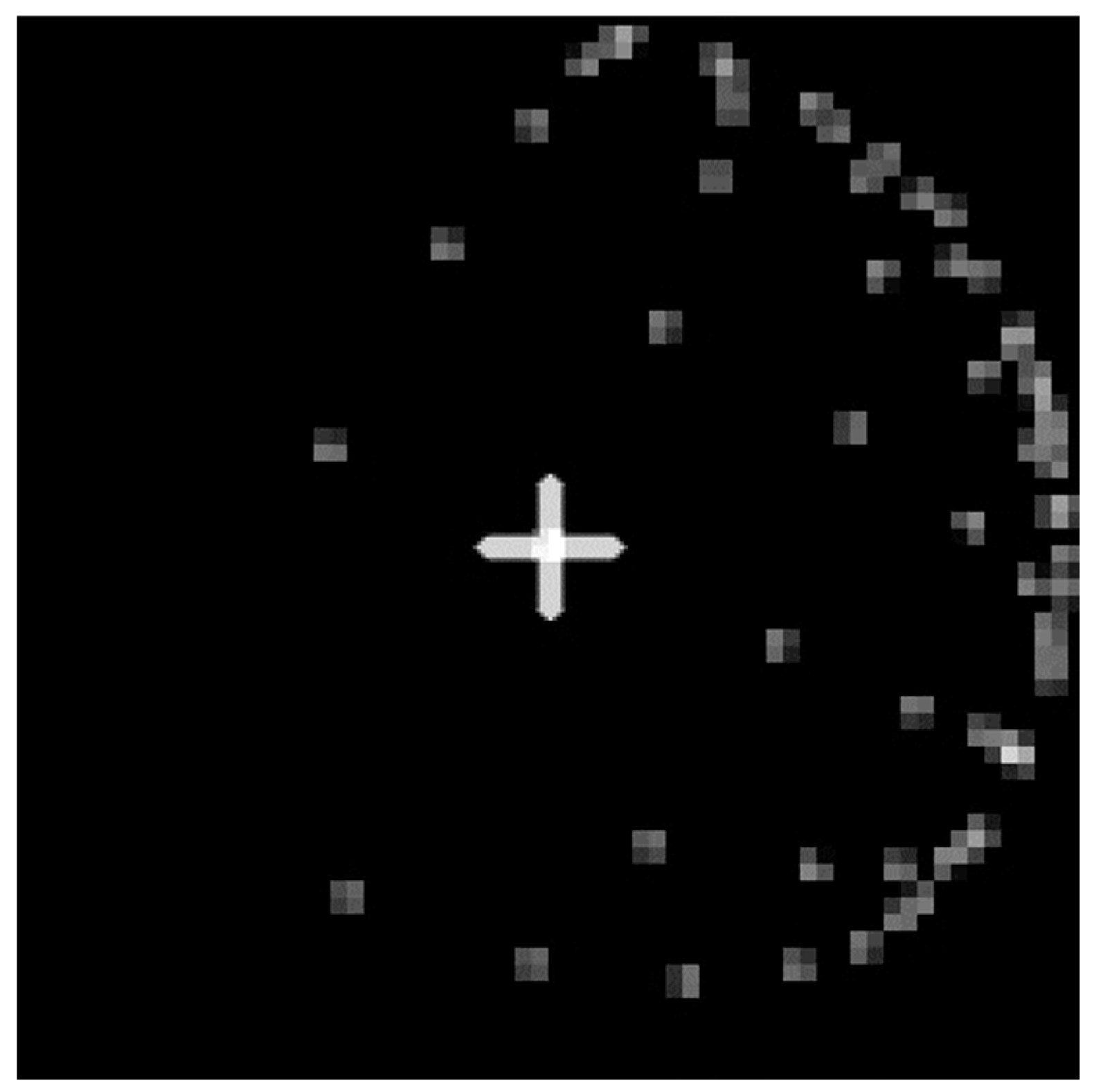
In tandem, the second image, designated as the boresight image, offers a more focused perspective, featuring a layer of a 64 × 64 pixel grid, as shown in Figure 5. These layers represent observation targets in close proximity to the telescope boresight, utilizing local coordinates of angular separation along the x and y axes. This layer imparts information about the spatial distribution of observation targets in relation to the boresight.

Beyond the aforementioned spatial information, the observation space also included non-spatial features in the form of 7 32-bit floating-point numbers. These numbers indicate the remaining simulation steps and the last actions for the x and y axes within the range of [1, 1], as detailed in

Table 2. Non-spatial features.

Description	Value Range	Encoded Range
Remaining simulation steps	[0, ∞), capped at 4096	[0, 1]
X action at t−1	[−1, 1]	[−1, 1]
Y action at t−1	[−1, 1]	[−1, 1]
X action at t−2	[−1, 1]	[−1, 1]
Y action at t−2	[−1, 1]	[−1, 1]
X action at t−3	[−1, 1]	[−1, 1]
Y action at t−3	[−1, 1]	[−1, 1]

Within the blue layer, designated as the telescope information layer, the current telescope boresight location is denoted by a rectangular patch of 10 degrees per side. The location of the telescope boresight is projected by the telescope electric servomotor model, taking into account internal and external perturbations to the telescope, as further described in Section 2.3.3. In a real-world scenario, the angles from the rotary encoders on both axes are to be directly employed. These angles of the X-Y pedestal are converted into azimuth and elevation, as demonstrated in Section 2.1.2.

Concurrently, the green layer illustrates telescope observation targets, encompassing celestial bodies or regions of interest. The position of each target is represented by 4 pixels, and the relative intensity of each pixel is proportional to the target position. The celestial coordinates of each target were obtained and subsequently transformed to local coordinates of azimuth and elevation, incorporating the required atmospheric correction using the Astronomical Coordinate System’s modules from the Astropy library [26]. In the simulation, these coordinates are cached in a local database to prevent unnecessary recomputation and expedite the training process. The same database could be employed to store precomputed coordinates in a real-world scenario, alleviating computation workload. Target dwelling time can be adjusted to suit observation requirement.

The red layer within the spatial observation space is designated to represent RFI sources or other factors that impede telescope survey, manifested as patches or spots. This included space-based RFI sources such as geostationary communication satellites, low-Earth-orbit satellites, aircraft, and adverse atmospheric conditions such as precipitation and cloud coverage. RFI from geostationary communication satellites was modeled as stationary patches based on a comprehensive site survey.

RFI from aircraft was dynamically modeled. The aircraft trajectories (speed, altitude, heading) were captured during a 7-day survey at the site. The aircraft position in the sky image was updated at every simulation timestep using information stored in a database for that day of the week. Simulated aircraft could also be incorporated to provide stochasticity. In this case, simplified flight dynamics models were employed to simulate their movement across the sky. For meteorological conditions, weather radar images from Suvarnabhumi Airport and the Bangkok metropolitan area are used.

The boresight layers represent observation targets in the vicinity of the telescope boresight. Observation targets are filtered out so only those within 10 degrees of the boresight are shown. The telescope boresight is fixed at the center and the x and y axes of the image are aligned with those of the telescope. Each target is represented by pixels in a similar manner to the green layer. Angular separation is scaled with a hyperbolic tangent function to provide higher resolution closer to the boresight while maintaining a wide field of view.

2.3.2. Action Space

The action space of this simulated environment had two degrees of freedom: one for the servomotor on the primary axis and another for the secondary axis. The input range for both axes is continuous [−1, 1], with −1, 0, and 1 corresponding to maximum reverse speed, stop, and maximum forward speed, respectively.

In the simulated environment, the input signal was sent to the servomotor model, which subsequently calculated the spin-up time based on the motor load and external perturbation. Subsequently, the model returned the updated position of the radio telescope axes to the simulator.

2.3.3. Telescope Model

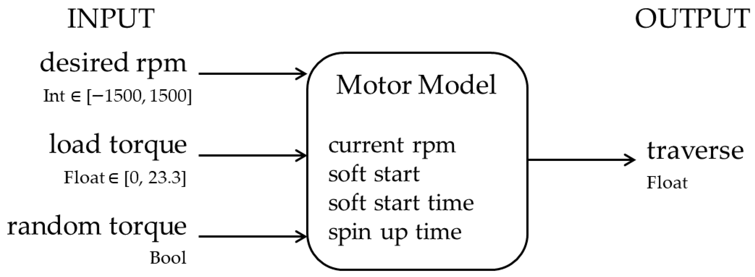
The electric servomotor model is initialized with the motor parameters outlined in Section 2.1.3, with the option of a soft start. Upon initialization, the model stands ready to receive input parameters, namely the desired revolutions per minute (rpm), load torque, and whether to use random torque. The range of rpm input is continuous at [−1500, 1500] and [0, 23.3] for the load torque, where 23.3 N·m. corresponds to the peak torque of the current drive train setup.

The inclusion of a random torque flag serves to introduce variability into the load torque exerted on the servomotor, thereby providing an additional layer of realism essential for domain randomization. When enabled, the model is initialized with a random load torque coefficient from a uniform distribution [−0.5, 0.5] that is reset at the beginning of each episode. These torque coefficient values vary between the motors, episodes, and parallel environments. Additionally, the torque is subject to random, transient resampling during the episode to represent temporary torque changes with the objective of simulating transient events such as a wind gust or sudden friction changes. The probability of this transient reset is set at a default of P(resample) = 0.005.

During runtime, the electric servomotor model dynamically processes these inputs, computing the resultant spin-up time and cruising time in alignment with the simulation timestep. This computation eventually returns the total distance traversed as its output, which is then used to update the radio telescope’s boresight location. The functionality of the electric servomotor model is illustrated in Figure 6.

2.4. Telescope Control Model

2.4.1. Model Structure

The RL agent was implemented entirely in Python utilizing the PyTorch 2.0 framework. The implementation closely followed the original PPO implementation with some modifications: the incorporation of generalized state-independent exploration and the exclusion of entropy loss for exploration. In our specific case, the deterministic action was output from the actor network, combined with noise sampled periodically every 128 steps from a fixed normal distribution. The integration of this noise element aimed to introduce stochasticity, thereby enhancing the exploration capability of the RL agent while maintaining smooth action. The critic network was trained against the expected return to predict a return estimate for each observation, serving as a baseline to compute the advantage estimate and update the policy.

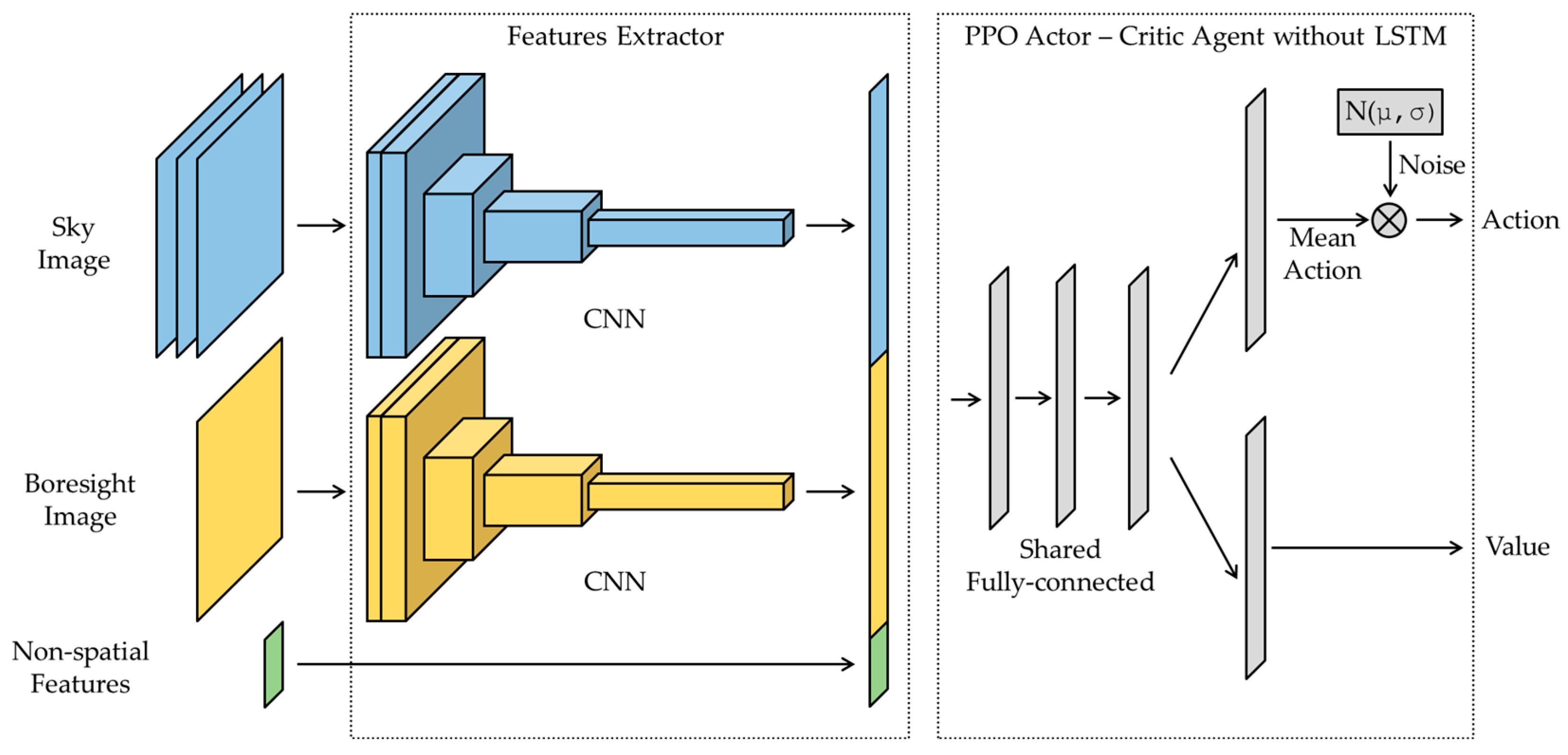
The telescope control model utilized two Convolutional Neural Network (CNN) feature extractors, each dedicated to processing one of the input images. These feature extractors served to condense the feature space, reducing model complexity and accelerating training, all while retaining spatial awareness to enhance overall performance. The outputs from these feature extractors were flattened and concatenated with the non-spatial features for the subsequent process by the PPO agent.

Three variants of the learning agent were studied. The first variant was a baseline agent with deep feedforward layers to further extract the spatial features followed by two separate feedforward layers for the mean action and the state-value estimate. A generalized state-independent exploration noise was added to the mean action, obtaining the action A_t. The architectural representation of the model is illustrated in Figure 7.

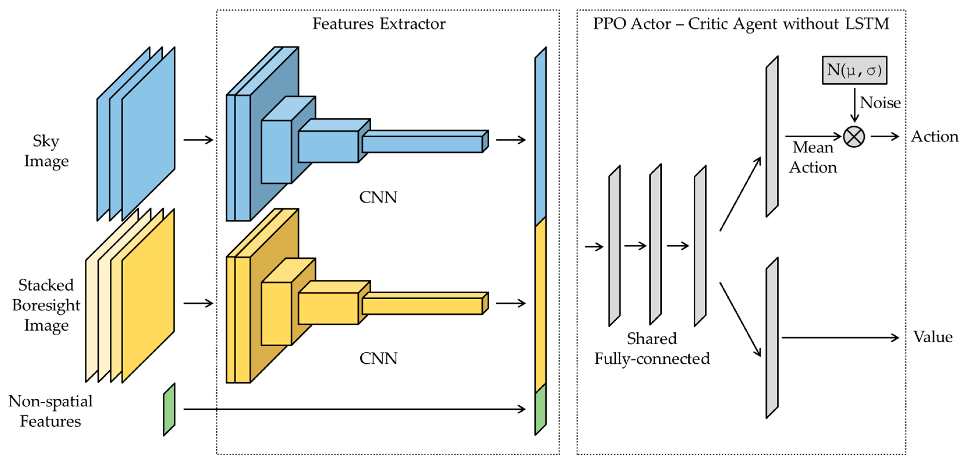
The second agent introduced basic temporal awareness through frame stacking. Four consecutive boresight images were stacked and processed by the feature extractor, yielding the same feature count as the first variant. The subsequent layers are the same as those in the first variant. The architectural representation of the model is shown in Figure 8.

The last variant used the same single deep feedforward layers to extract the spatial features, followed by a Long Short-Term Memory (LSTM) network to extract time-dependent features, contributing to the model’s ability to understand and adapt to the temporal patterns of the environment. The LSTM-processed features were then fed into separate feedforward layers for the mean action and the state-value estimate. The same generalized state-independent exploration noise was added to the mean action to obtain the action. The model architecture is demonstrated in Figure 9.

Long Short-Term Memory (LSTM) networks were chosen as a crucial component of the telescope control model due to their ability to capture and process sequential information effectively. Unlike traditional recurrent neural networks (RNNs), LSTMs are designed to mitigate the vanishing gradient problem, allowing them to retain information over extended sequences. In the context of the telescope control model, LSTMs played a pivotal role in understanding the temporal dynamics of the environment, enabling the model to make informed decisions based on the sequence of observations.

To efficiently initialize the CNN feature extractors, each was pre-trained in a supervised multi-task prediction network (Figure 10). This pre-training leveraged sky images generated at runtime with high diversity to learn a robust representation. The network was trained to predict two primary elements from the input image:

• Antenna location: the boresight’s local coordinates (X ∈ [−1, 1], Y ∈ [−1, 1]);
• Target cluster information: attributes for up to 8 target clusters, including their position, size, and obstructed status. Specifically, this consisted of cluster coordinates (X ∈ [−1, 1], Y ∈ [−1, 1]) and normalized cluster size (size ∈ [−1, 1]). Target clusters outside of the telescope horizon were masked out, and obstructed target clusters were given a negative size to encode their unobservable status.

For optimization, a combined loss function was employed. Mean Squared Error (MSE) was used as the loss function for the antenna location prediction, treating it as a standard regression task. For the target clusters, the Chamfer Distance was utilized, as the clusters were treated as a point cloud, where each point had 3 degrees of freedom (x position, y position, and size). The combined MSE loss and Chamfer Distance were then used to optimize the feature extractor network weights prior to the RL training phase. The architecture of the CNN feature extractor is detailed in

Table 3. The CNN feature extractor’s architecture.

Layer	Species	Size of Output	Parameters
0	Input Layer	64 × 64 × 3 1
1	Conv2d, ReLU	64 × 64 × 32	3 × 3
2	Conv2d, ReLU	64 × 64 × 64	3 × 3
3	Maxpool2d	32 × 32 × 64	2 × 2
4	Conv2d, ReLU	32 × 32 × 128	3 × 3
6	Maxpool2d	16 × 16 × 128	2 × 2
7	Conv2d, ReLU	16 × 16 × 256	3 × 3
8	Maxpool2d	8 × 8 × 256	3 × 3
9	Conv2d, ReLU	8 × 8 × 256	3 × 3
10	Maxpool2d	4 × 4 × 256	2 × 2
11	Conv2d, ReLU	1 × 1 × 256	4 × 4
12	Flatten	256

¹ 64 × 64 × 1 for boresight images.

.

2.4.2. Model Training

The model was trained in sixteen asynchronous vectorized environments. Each environment was initialized with different characteristics, such as the number of target clusters, obstacle, telescope angles, time of day, and load torque. The ranges for each characteristic are listed in

Table 4. Simulated environment initialization.

Parameters	Range	Type
Random Load Torque Flag	True, False	Boolean
Random Time Flag	True, False	Boolean
Random Telescope Angle Flag	True, False	Boolean
Random Load Torque Magnitude	[−0.2, 0.2]	Float
Number of Target Clusters	1–4	Integer
Target Dwell Time (s)	1–60	Integer
Number of Interference Sources	0–4	Integer
Time	Unix Timestamp	Integer
Telescope X Angles (deg)	[−80, 80]	Float
Telescope Y Angles (deg)	[−80, 80]	Float

.

During the rollout phase, the agent interacted with the environment at a rate of one action per second. There were two conditions for episode termination: empty sky, triggered when there was no observable target left, and truncation, which occurred when the agent completed 16,384 steps in the current episode, signaling that further training in similar conditions would yield limited benefits. Following termination, the expected return and advantage estimate for each step were computed and stored in the rollout buffer, alongside observations, actions, action probabilities, rewards, and value estimates. The environment was then reset and repeated until the rollout buffer of 32,768 steps was filled, marking the start of the training phase.

During the training phase, the rollout buffer was shuffled and restructured into 16 minibatches of 2048 steps. This was then used to update the actor network and critic network in accordance with the PPO algorithm described in Section 2.2. Each buffer was used to train the agent up to 10 times. An entropy loss was not employed to regulate the agent exploration as the exploration noise was sampled from a fixed normal distribution periodically every 128 steps. Upon the completion of the training phase, the algorithm transitioned back to the rollout phase. The hyper-parameters for the PPO are denoted in

Table 5. PPO hyperparameters.

Parameters	Value
Optimizer	Adam
Learning Rate	5 × 10−5
Annealing Learning Rate	False
Discount Factor	0.99
GAE	True
GAE Lambda	0.95
PPO Clip Ratio	0.2
Target KL	None
Clip Value Loss	True
Value Loss Coefficient	0.5
Max Gradient Normalization	0.5
Rollout Buffer	32,768
Minibatch Size	2048
Environment Count	16
Exploration Noise	0.2

The training was performed on a CUDA-accelerated system with an NVIDIA GeForce RTX 3060 GPU (12 GB of GPU memory) and an AMD Ryzen 5 5600, requiring approximately 84 h to reach 100 million training steps for the non-recurrent agent. The same configuration required more than 200 h to reach the same training steps for the recurrent agent.

.

2.4.3. Reward Shaping

The main reward for the model is obtained by completely surveying the sky, with an additional reward proportional to the remaining simulation steps. This ultimate sky-clearance reward, however, is inherently sparse and is unlikely to be achieved by a random agent in the exploration process.

To address the sparsity, the second main reward is introduced. This target clearance reward is obtained when the telescope successfully maintains its boresight over an observation target for the required dwell time. A target can be observed only when it is not obstructed by interference sources and the telescope is not out of bounds. While this reward is more attainable than the sky clearance reward, it still presents a degree of sparsity.

To further accelerate the learning process, reward shaping has been employed. This involves giving small, immediate rewards for performing trivial tasks that contribute to the main objective. Specifically, a small reward is given proportionally to the angular distance the telescope traverses depending on its closeness to the closest observation target. A slightly higher penalty is applied if the telescope moves away from the closest target.

This minuscule, instantaneous reward structure helps guide the agent to make incremental progress toward clearing targets while still allowing it to perform the necessary exploration. The overall reward structure and conditions are as shown in

Table 6. Reinforcement learning reward structure.

Name	Condition	Reward
Sky clearance	No targets over the horizon. Successfully observed any target.	0.0025 per remaining steps. Capped at 10.
Target clearance	Uninterruptedly maintaining a target inside boresight during the dwell time.	1
Target approach	Angular distance to the closest unobstructed target.	0.010 per mrad (closer) 0.011 per mrad (further)

.

2.5. Evaluation

2.5.1. Performance Metrics

The comprehensive performance of the proposed agent was evaluated by quantifying the effective celestial sphere solid angle that the telescope could cover, measured in square degrees per hour (deg²/h). This assessment aimed to gauge the speed and adaptability of the DRL agent in optimizing telescope movements and target selection, particularly under dynamic RFI conditions. As a practical benchmark for comparison, the DRL agent’s performance was measured against a proportional controller agent, which was programmed to systematically follow the closest observation target without considering potential interference sources. The parameters of this proportional agent were tuned to maximize survey coverage via Stochastic Gradient Descent (SGD) optimization.

2.5.2. Feature Extractor Evaluation

The evaluation of feature extractors involved a comparative analysis of our custom implementation against a similar feature extractor based on the 3-layer CNN architecture from NatureCNN [27]. The latter previously demonstrated its ability to achieve human-level control in an Atari game using image input. Notably, the baseline feature extractor was configured to produce the same number of features as our proposed feature extractor. This ensured a fair comparison of the architectural impacts, keeping the downstream network components and the total computational complexity consistent.

Furthermore, the necessity of the supervised pre-training component was tested in an ablation study. This involved comparing the performance of a non-recurrent agent utilizing the pre-trained feature extractor against a similar agent initialized with random feature extractor weights.

2.5.3. Agent Evaluation

For the evaluation of the learning agent, the pre-trained custom feature extractor was utilized in every agent. The primary goal was to quantify the impact of incorporating temporal awareness, with two baselines chosen for this study.

The first baseline consisted of an agent without any explicit temporal awareness, where the concatenated output from the feature extractors was directly fed into the actor and critic network, serving as a performance benchmark.

The second baseline introduced basic temporal awareness through frame stacking, where four boresight observations were stacked together, resulting in four sets of images. Each set of images was processed by a modified feature extractor and subsequently passed through a fully connected layer where feature count was reduced to match that of a single observation case.

These two baselines were used as benchmarks to evaluate the efficacy of the proposed recurrent agent utilizing Long Short-Term Memory (LSTM) cells. The resulting performance comparison directly quantifies the contribution of explicit memory to the policy’s robustness and efficiency in managing dynamic RFI and long-horizon telescope scheduling.

2.5.4. Real-World Performance

The learned agent’s policy was transferred to the real telescope system to validate its real-world applicability. The control interface and data acquisition were set up as follows:

• Observation: The telescope boresight position was taken directly from the telescope encoders through UDP broadcast. Observation target coordinates were calculated in real time, and the obstacle layer was generated from real-time ADS-B feeds and weather radar.
• Action: The servomotor was configured to operate in speed control mode. The action output from the DRL agent was transmitted to the Servopack through a Modbus RTU analog output module. This analog output module transmitted a voltage signal in the range of [−3, 3] V, which corresponded to the servomotor’s operational rpm range of [−1500, 1500] rpm.

The effective survey coverage obtained from the real environment was then compared against the results from the simulated environment to assess the real-world transferability of the policy.

3. Results

3.1. Performance of Feature Extraction Baselines

The initial evaluation phase validated the architectural performance of the Custom CNN Feature Extractor against the standard NatureCNN baseline. Both networks were subjected to identical supervised pre-training, utilizing a multi-task objective comprising Mean Squared Error (MSE) for boresight localization and Chamfer Distance for target cluster prediction.

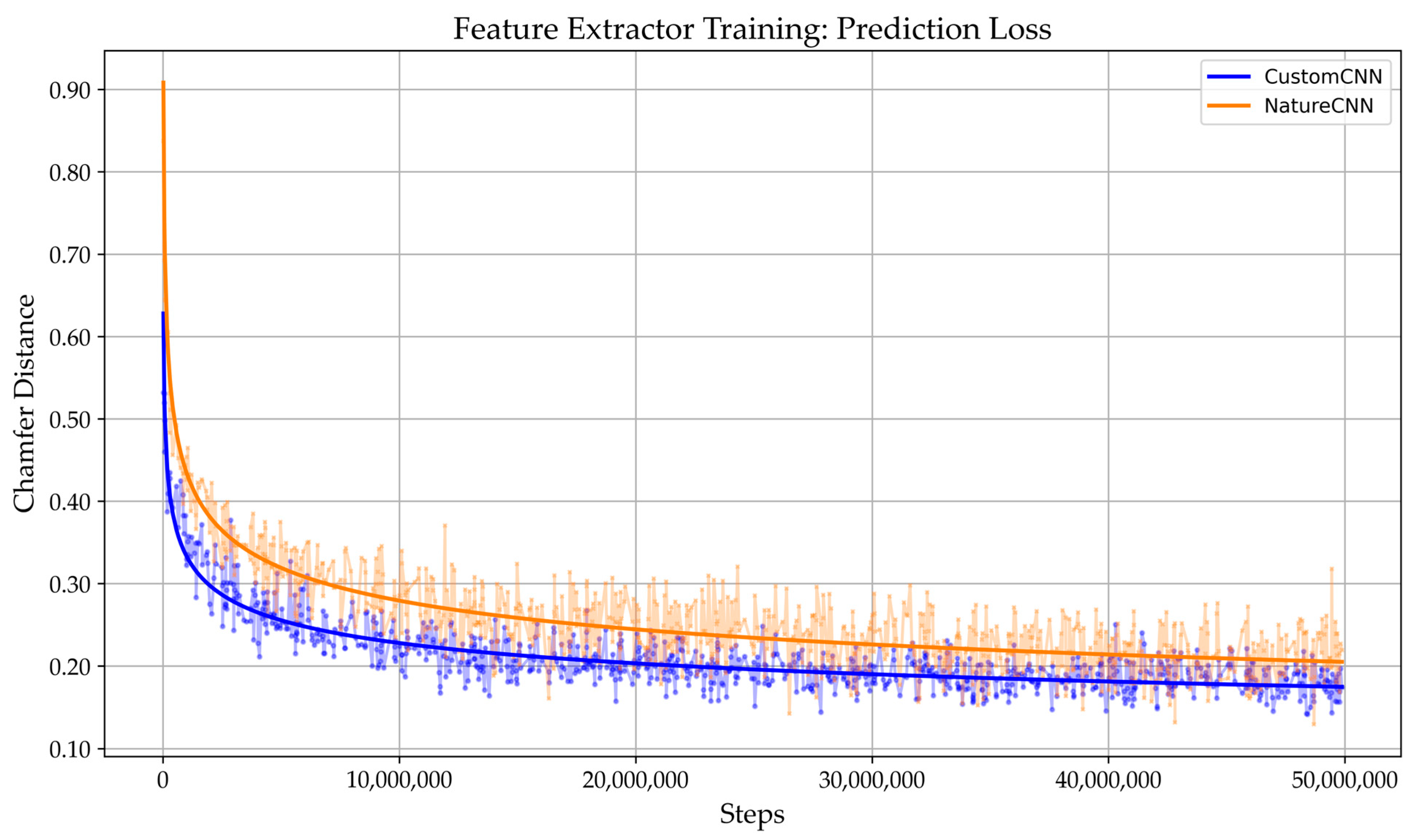
As presented in Figure 11, the convergence rates for both feature extractors were comparable. However, the Custom CNN architecture achieved a significantly and consistently lower final prediction loss across both tasks compared to the NatureCNN. This performance disparity is quantified by the final convergence loss metrics.

Focusing on the Chamfer Distance component of the loss, which assesses the accuracy of the extracted target cluster information, the performance disparity is apparent. The NatureCNN converged to a final loss value of approximately 0.21. In contrast, the Custom CNN yielded a lower loss, converging to approximately 0.16. This consistent and lower prediction loss demonstrated by the Custom CNN confirms its ability to extract a higher-fidelity, domain-specific feature representation of the complex image state.

Comparing the performance of the feature extractors, the NatureCNN architecture achieved a survey coverage of 234 deg²/h, whereas the CustomCNN achieved a higher mean survey coverage of 275 deg²/h in the non-recurrent agent, confirming the superior feature extraction capability of the domain-specific architecture. Neither feature extractor converged when initialized without supervised pre-training. The CustomCNN exhibited a slightly slower convergence than the NatureCNN.

Table 7. Impact of feature extractor architecture and supervised pre-training.

Feature Extractor	Pre-Training	Training Steps to Convergence	Mean Survey Coverage (deg2/h)
NatureCNN	No	No	-
CustomCNN	No	No	-
NatureCNN	Yes	6 million	234
CustomCNN	Yes	7 million	275

summarizes the performance metrics and convergence times for the non-recurrent agent when utilizing the NatureCNN and CustomCNN architectures.

3.2. Impact of Temporal Awareness

The second phase of evaluation quantified the benefit of incorporating memory and temporal awareness into the policy architecture. Three agents, all utilizing the validated Custom CNN Feature Extractor (Section 3.1), were compared: the non-recurrent baseline, the frame stacking agent, and the proposed recurrent agent (LSTM). Performance was measured by the final average effective survey coverage in deg²/h.

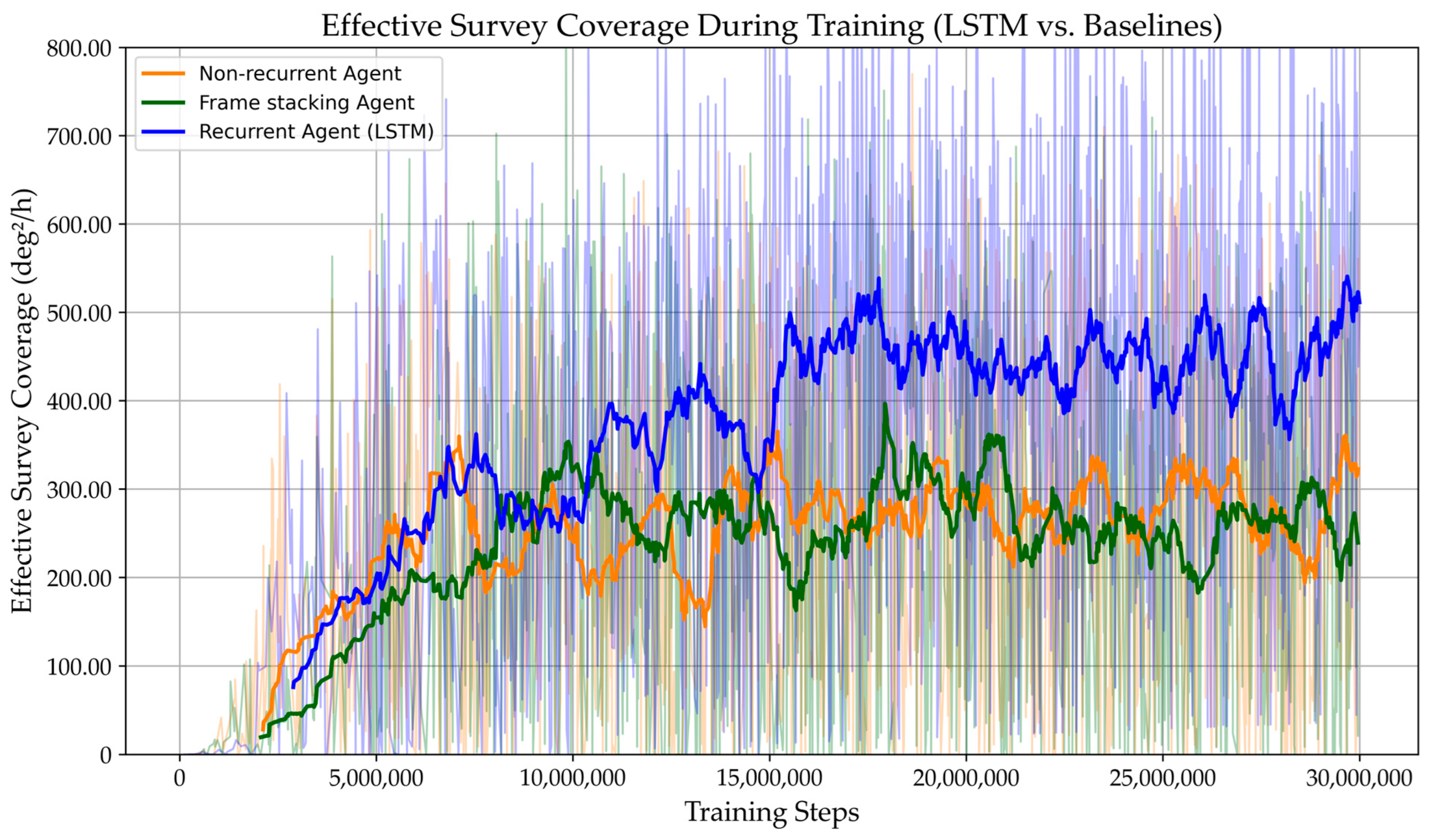
As shown in the learning curves (Figure 12), the introduction of recurrence significantly influenced training dynamics and final policy efficacy. The recurrent agent (LSTM) achieved the highest final average reward, while the non-recurrent and frame stacking agents converged at a lower performance. An ablation of the pre-trained feature extractor was also studied.

The final performance metrics, derived from the sustained average reward near the end of the training phase (after 20,000,000 steps), are summarized in

Table 8. Survey coverage and convergence metrics for DRL architectural variants.

Agent Architecture	Training Steps to Convergence	Mean Survey Coverage (deg2/h)	Relative Improvement (vs. Non-Recurrent)
Non-recurrent	7 million	275	N/A
Frame Stacking	10 million	270	−2.1%
Recurrent	18 million	475	72.7%

:

The recurrent agent achieved the highest effective survey coverage, sustaining a final average of 475 deg²/h. This demonstrates a substantial 72.7% superiority over the non-recurrent baseline (275 deg²/h). Notably, the frame stacking agent (270 deg²/h) presented no significant improvement against the non-recurrent baseline while taking more training steps (10 million steps against 7 million) to reach convergence.

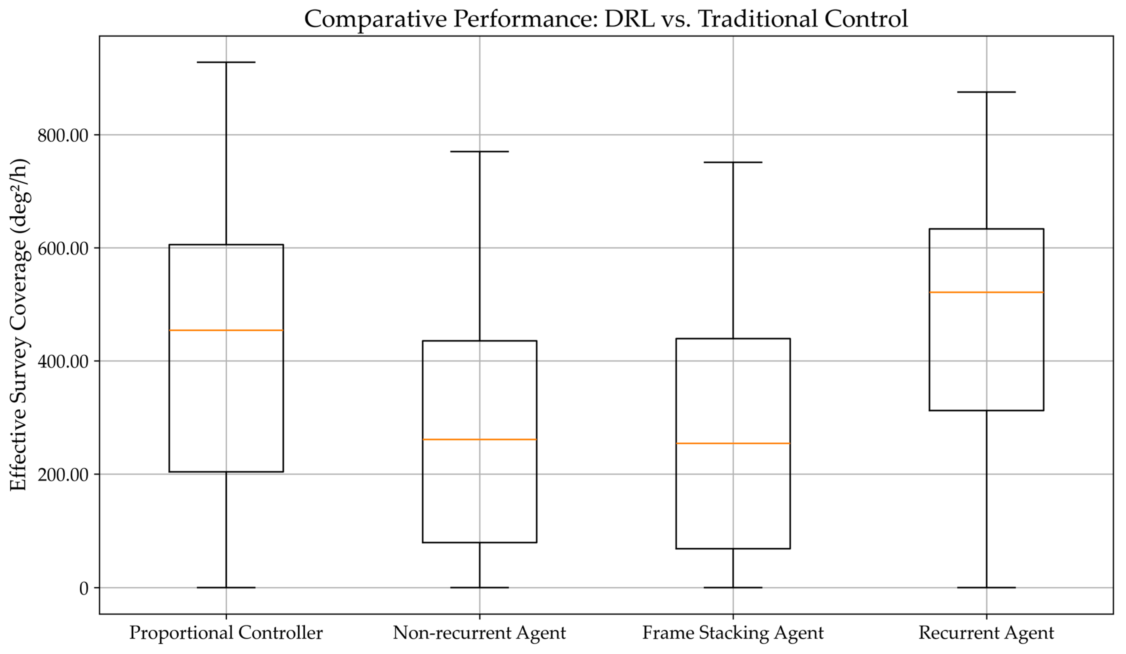
The final evaluation benchmarked the optimal DRL configuration, the recurrent agent (LSTM), against the traditional proportional controller and the two DRL baselines (non-recurrent and frame stacking). The results, presented as box plots in Figure 13, show the statistical distribution of effective survey coverage (deg²/h) achieved across multiple simulation scenarios. This visualization highlights not only the central tendency but also the variability and reliability of each controller’s performance.

The result confirmed the superior performance and stability of the recurrent architecture. The recurrent agent (LSTM) achieved the highest median survey coverage (Q2) of 521 deg²/h, surpassing the proportional controller (454 deg²/h), the non-recurrent agent (261 deg²/h), and the frame stacking agent (254 deg²/h).

The recurrent agent also demonstrated superior statistical reliability, evidenced by the lowest Interquartile Range (IQR) of 321 deg²/h. This tighter distribution confirms the recurrent agent’s consistent and robust performance across the complex RFI scenarios compared to the proportional controller (402 deg²/h), the non-recurrent agent (355 deg²/h), and the frame stacking agent (370 deg²/h).

The consistency of the recurrent agent is also reflected in its high lower quartile (Q1) of 312 deg²/h. This value significantly exceeds the Q1 of the non-recurrent agent (80 deg²/h) and the frame stacking agent (69 deg²/h), demonstrating that the recurrent agent maintained a higher baseline efficiency across its less optimal operational conditions. While the traditional proportional controller achieved the highest single peak performance of 928 deg²/h, indicating high potential in optimal conditions, the recurrent agent maintained a robust peak of 876 deg²/h. The finding that the recurrent agent sustained a significantly higher Q1 and median validates its overall reliability and consistency, establishing its superiority for RFI-aware dynamic scheduling.

The statistical distribution of performance across all four control strategies is also presented in

Table 9. Statistical distribution of performance across all four control strategies in the simulated environment.

Metric	Proportional Controller	Non-Recurrent Agent	Frame Stacking Agent	Recurrent Agent (LSTM)
Q1	204	80	69	312
Q2	454	261	254	521
Q3	606	435	439	633
IQR	402	355	370	321
Min	0	0	0	0
Max	928	770	751	876

. This analysis benchmarked the performance of the recurrent agent against the establish baselines.

3.3. Sim-to-Real Policy Transfer

The final phase of the evaluation involved validating the performance of the three DRL policies in the real environment interfacing with the telescope hardware. This experiment assessed the real-world transferability of the policies by comparing the Effective Survey Coverage achieved in the real environment against the sustained average performance recorded in the simulation. The comparison quantifies the reality gap, defined as the performance degradation resulting from discrepancies between the simulated environment and the real environment. The comparison of statistical performance metrics between the simulated and real environments is detailed in

Table 10. Statistical distribution of real-world performance in comparison with the simulation.

Metric	Proportional Controller		Non-Recurrent Agent		Frame Stacking Agent		Recurrent Agent (LSTM)
	Deg2/h	Change	Deg2/h	Change	Deg2/h	Change	Deg2/h	Change
Q1	167	−18.1%	80	0%	80	+15.9%	301	−3.5%
Q2	391	−13.9%	229	−12.3%	262	+3.1%	516	−1.0%
Q3	587	−3.1%	392	−9.7%	424	−3.4%	631	−0.3%
IQR	420	+4.5%	312	−11.8%	344	−7.0%	330	+2.8%
Min	0	0.0%	0	0.0%	0	0.0%	0	0.0%
Max	866	−6.7%	727	−5.6%	774	+3.1%	880	+0.5%

.

The non-recurrent agent experienced a 12.3% reduction in median effective survey coverage compared to its simulated performance. This drop in performance quantifies the reality gap for the policy lacking temporal awareness. In contrast, both the frame stacking agent and the recurrent agent (LSTM) showed less performance deterioration in the real environment. Specifically, the recurrent agent (LSTM) maintained exceptional stability with only a 1.0% decrease in median coverage.

4. Discussion

4.1. Feature Extractor Validation and Architectural Impact

The pre-training results (Section 3.1) clearly demonstrated that the specialized architectural design of the Custom CNN provided a substantial advantage over the standard NatureCNN baseline. This was confirmed by the consistently lower prediction loss, particularly in the Chamfer Distance metric, which governs the accuracy of target cluster localization and RFI obstruction status. Since both networks were trained with an identical multi-task objective, the performance difference is directly attributable to the topology of the Custom CNN.

The NatureCNN architecture, while effective for similar tasks like Atari games, proved suboptimal for this application. The NatureCNN features relatively large kernels (8 × 8) in early layers to capture global image features quickly. This design is unsuitable for the telescope’s observation space, where crucial information can be represented by very small spatial features, sometimes as small as (2 × 2) pixels. A large kernel in the first layer risks averaging or obscuring this vital, fine-grained information.

The Custom CNN was tailored to the spatial characteristics of the sky images, benefiting from a greater depth and a more granular approach to feature extraction. This improvement in detecting small features is paramount, as the agent’s performance in the subsequent reinforcement learning process is dependent on receiving accurate state information regarding targets and RFI.

The full DRL training process further validated the architectural choice. The ablation study comparing the converged policies showed that the Custom CNN architecture ultimately yielded a mean survey coverage of 275 deg²/h in the non-recurrent agent, significantly surpassing the NatureCNN. Crucially, the ablation confirmed the necessity of supervised pre-training for the agent to achieve a functional policy within practical time constraints in these scenarios.

4.2. Validation of Recurrent Architecture and Final Implications

The impact of temporal awareness has validated the necessity of a deep reinforcement learning agent with both spatial and temporal awareness for this application, as the telescope controlling and scheduling task requires both precision in telescope movement and long-term planning for dynamic scheduling.

The short-term temporal awareness provided by frame stacking proved to be insufficient for the task. Frame stacking created additional training overhead, and the resulting layers did not contribute enough to policy performance to justify the increased computational complexity, underscoring the necessity of an explicit recurrent structure for complex, long-horizon decision-making.

The LSTM agent leverages its temporal awareness capability to achieve proactive RFI mitigation. By observing the trajectory of targets and RFI sources, the recurrent agent can predict future blockage, enabling dynamic switching of targets before interference arrives, maximizing the effective telescope survey time.

The final benchmark against the proportional controller demonstrated a key trade-off between classical and DRL control. The traditional controller achieved the highest peak performance of 928 deg²/h, distinguishing itself in terms of raw precision and speed in optimum operational conditions. Conversely, the recurrent agent, while presenting a slightly lower peak performance of 876 deg²/h (−5.6%), demonstrated superior performance and stability in every other metric.

This superior reliability is evidenced by the LSTM’s highest median coverage (521 deg²/h) and a tighter IQR (321 deg²/h), confirming that its RFI-aware scheduling and adaptive control lead to more consistent and robust performance across complex scenarios. This robustness is partly due to its ability in prioritizing time-essential targets and its capability to ignore unobservable targets.

4.3. Impact of Temporal Awareness in Sim-to-Real Policy Transfer

The successful sim-to-real policy transfer experiments further highlighted the stabilizing effect of temporal awareness against unmodeled real-world perturbations. The non-recurrent agent suffered a performance deterioration in the real environment. This drop is attributed to the policy’s inability to compensate for transient events or unmodeled lag (such as motor friction or wind gusts) that occurred in the last few steps before the full tracking error was visible.

Conversely, both the recurrent agent (LSTM) and the frame stacking agent showed minimum performance deterioration in the real environment. This stability validates that the memory-enabled agents, through their temporal encoding mechanisms, developed a robust policy capable of compensating for unmodeled uncertainties and transient events, successfully mitigating the reality gap. Nevertheless, the failure of the frame stacking agent to improve upon the non-recurrent baseline during training (Section 3.2) underscores that a true, explicit memory mechanism like the LSTM is required for long-horizon decision-making, even though implicit memory provided minor stability gains in the real environment.

4.4. Future Research Directions

While the recurrent agent (LSTM) demonstrated superior final performance and stability, its training process exhibited significantly lower sample efficiency compared to the baselines. The recurrent agent required 18 million training steps to converge, which is 11 million and 8 million steps more than the non-recurrent (7 million steps) and frame stacking (10 million steps) agents, respectively. This increase in training time is further aggravated by the increased architectural complexity of the LSTM layer, which introduces more parameters, nodes, and temporal dependencies requiring optimization. In our implementation, this complexity resulted in the LSTM agent running more than twice as slow as the non-recurrent and frame stacking agents.

For larger, more complex DRL problems, this significant increase in training time could make training the recurrent agent from scratch computationally infeasible. To mitigate this sample inefficiency and accelerate the training of robust recurrent policies, a promising future research avenue is to explore a two-stage training methodology. This approach would first train the network without the recurrent layer until initial convergence and then incorporate the LSTM layer in a second stage to fine-tune the long-horizon planning and temporal awareness, potentially drastically reducing the total time required to reach the optimum recurrent policy.

Other research avenues could focus on three primary directions to advance the robustness, planning capabilities, and real-world applicability of this DRL framework.

The first direction should focus on exploring a Hybrid DRL Control Architecture. This involves leveraging the inherent strengths of both classical and learned control by integrating the high-precision capabilities of the traditional proportional controller for low-level, high-frequency motor control. This architecture would utilize the DRL layer to operate at a lower frequency, handling dynamic scheduling, RFI avoidance, and target prioritization. This effectively decouples the task into high-precision tracking (classical control) and strategic planning (DRL), thereby capitalizing on the high peak performance of traditional control while retaining the adaptability of the learned policy.

The second direction should focus on expanding the environment and agent to categorizing targets and RFI by their spectrum. The current model treats all RFI as an absolute obstruction, requiring target avoidance regardless of the observation band. By integrating spectral information (e.g., L-band, S-band, X-band), the agent can be trained to dynamically adjust the survey frequency or continue observation if the interference source is operating outside the target’s frequency band. This advanced scheduling capability will significantly increase valuable observation time and survey efficiency in a multi-band radio astronomy system.

The third direction involves conducting further systematic methodological ablation studies to maximize performance and refine generalization capabilities. While the current work validated the necessity of the feature extractor and the recurrent memory core, future research should systematically investigate the impact of other key hyper-parameters and design choices, such as reward structure sensitivity, exploration noise schedules, and the specific impact of the various domain randomization parameters. This detailed methodological investigation will be essential for optimizing the DRL policy for general deployment across varied telescope sites and environments.

5. Conclusions

This study successfully implemented a Deep Recurrent Reinforcement Learning (DRL) framework for radio telescope control and dynamic scheduling in a simulated environment modeled on the RFI-laden conditions of the KMITL radio telescope. The evaluation rigorously tested the contributions of specialized architecture, memory, and traditional control baselines.

The results confirm the necessity of domain-specific architectural design. The Custom CNN Feature Extractor significantly outperformed the standard NatureCNN in pre-training by achieving a lower prediction loss. This validated the approach of tailoring the feature extraction topology to the unique characteristics of the sparse, high-information-density sky images.

The inclusion of a temporal awareness mechanism was critical. The recurrent agent (LSTM) achieved a substantial 72.7% superiority in average effective survey coverage over the non-recurrent baseline, confirming that the task requires long-horizon planning and temporal awareness. This architecture’s capacity for proactive RFI mitigation and long-term scheduling led to its superior performance in the final benchmark.

The final evaluation confirmed the DRL framework as a highly competitive and robust control solution:

• The LSTM policy achieved the highest median survey coverage of 521 deg²/h, surpassing the traditionally tuned proportional controller.
• The LSTM demonstrated superior reliability, evidenced by the tightest interquartile range (321 deg²/h) among all agents, confirming its consistent robustness across complex, unpredictable scenarios.

Finally, the sim-to-real policy transfer validated the robustness of the memory-enabled policies, as the recurrent agent showed minimal performance deterioration in the physical environment, successfully mitigating the reality gap against unmodeled dynamics and transient events.

In conclusion, the proposed DRL framework offers a reliable, adaptive, and high-performance solution for radio telescope scheduling, capable of maintaining survey efficiency while proactively managing RFI sources. Future work should focus on advancing this foundation through hybrid control architectures and expanding the environment to include spectral categorization of targets and RFI to further optimize observation time.

References

1. Bhat, N.; Swainston, N.; McSweeney, S.; Xue, M.; Meyers, B.; Kudale, S.; Dai, S.; Tremblay, S.; Van Straten, W.; Shannon, R.; et al. The Southern-sky MWA Rapid Two-metre (SMART) pulsar survey—I. Survey design and processing pipeline. Publ. Astron. Soc. Aust. 2023, 40, 1–22. [Google Scholar] [CrossRef]
2. Buchner, J. Dynamic Scheduling and Planning Parallel Observations on Large Radio Telescope Arrays with the Square Kilometre Array in Mind. Master’s Thesis, Auckland University of Technology, Auckland, New Zealand, 2011. [Google Scholar]
3. Shyalika, C.; Silva, T.; Karunananda, A. Reinforcement Learning in Dynamic Task Scheduling: A Review. SN Comput. Sci. 2020, 1, 306. [Google Scholar] [CrossRef]
4. Baan, W. RFI mitigation in radio astronomy. In Proceedings of the General Assembly and Scientific Symposium, Groningen, The Netherlands, 29–31 March 2011; pp. 1–2. [Google Scholar]
5. Colome, J.; Colomer, P.; Guàrdia, J.; Ribas, I.; Campreciós, J.; Coiffard, T.; Gesa, L.; Martínez, F.; Rodler, F. Research on schedulers for astronomical observatories. In Proceedings of the SPIE—The International Society for Optical Engineering, Amsterdam, The Netherlands, 1–2 July 2012; Volume 8448. [Google Scholar] [CrossRef]
6. Huang, C.-N.; Chung, A. An Intelligent Design for a PID Controller for Nonlinear Systems. Asian J. Control. 2014, 18, 447–455. [Google Scholar] [CrossRef]
7. Ghahramani, A.; Karbasi, T.; Nasirian, M.; Sedigh, A.K. Predictive Control of a Two Degrees of Freedom XY robot (Satellite Tracking Pedestal) and comparing GPC and GIPC algorithms for Satellite Tracking. In Proceedings of the 2nd International Conference on Control, Instrumentation and Automation, Shiraz, Iran, 27–29 December 2011; pp. 865–870. [Google Scholar]
8. Zhao, X.K.; Wang, H.; Tian, Y. Trajectory Tracking Control of XY Table Using Sliding Mode Adaptive Control Based on Fast Double Power Reaching Law. Asian J. Control. 2016, 18, 2263–2271. [Google Scholar] [CrossRef]
9. Sutton, R.S.; Barto, A.G. Reinforcement Learning: An Introduction, 2nd ed.; The MIT Press: Cambridge, MA, USA, 2018; p. xxii. [Google Scholar]
10. Mnih, V.; Kavukcuoglu, K.; Silver, D.; Graves, A.; Antonoglou, I.; Wierstra, D.; Riedmiller, M. Playing Atari with Deep Reinforcement Learning. arXiv 2013, arXiv:1312.5602. [Google Scholar] [CrossRef]
11. Song, Y.; Steinweg, M.; Kaufmann, E.; Scaramuzza, D. Autonomous Drone Racing with Deep Reinforcement Learning. In Proceedings of the 2021 IEEE/RSJ International Conference on Intelligent Robots and Systems (IROS), Prague, Czech Republic, 27 September–1 October 2021. [Google Scholar]
12. Weisz, G.; Budzianowski, P.; Su, P.H.; Gašić, M. Sample Efficient Deep Reinforcement Learning for Dialogue Systems with Large Action Spaces. IEEE/ACM Trans. Audio Speech Lang. Process. 2018, 26, 2083–2097. [Google Scholar] [CrossRef]
13. Andersson, J.; Bodin, K.; Lindmark, D.; Servin, M.; Wallin, E. Reinforcement Learning Control of a Forestry Crane Manipulator. arXiv 2021, arXiv:2103.02315. [Google Scholar] [CrossRef]
14. Mienye, I.D.; Swart, T.G.; Obaido, G. Recurrent Neural Networks: A Comprehensive Review of Architectures, Variants, and Applications. Information 2024, 15, 517. [Google Scholar] [CrossRef]
15. García, J.; Fernández, F. A comprehensive survey on safe reinforcement learning. J. Mach. Learn. Res. 2015, 16, 1437–1480. [Google Scholar]
16. OpenAI; Akkaya, I.; Andrychowicz, M.; Chociej, M.; Litwin, M.; McGrew, B.; Petron, A.; Paino, A.; Plappert, M.; Powell, G.; et al. Solving Rubik’s Cube with a Robot Hand. arXiv 2019, arXiv:1910.07113. [Google Scholar]
17. Peng, X.; Andrychowicz, M.; Zaremba, W.; Abbeel, P. Sim-to-Real Transfer of Robotic Control with Dynamics Randomization. arXiv 2017. [Google Scholar] [CrossRef]
18. Kaspar, M.; Munoz Osorio, J.D.; Bock, J. Sim2Real Transfer for Reinforcement Learning without Dynamics Randomization. arXiv 2020, arXiv:2002.11635. [Google Scholar] [CrossRef]
19. Schulman, J.; Wolski, F.; Dhariwal, P.; Radford, A.; Klimov, O. Proximal Policy Optimization Algorithms. arXiv 2017, arXiv:1707.06347. [Google Scholar] [CrossRef]
20. Schulman, J.; Levine, S.; Moritz, P.; Jordan, M.; Abbeel, P. Trust Region Policy Optimization. arXiv 2015, arXiv:1502.05477. [Google Scholar]
21. Brockman, G.; Cheung, V.; Pettersson, L.; Schneider, J.; Schulman, J.; Tang, J.; Zaremba, W. OpenAI Gym. arXiv 2016, arXiv:1606.01540. [Google Scholar] [CrossRef]
22. Raffin, A.; Hill, A.; Gleave, A.; Kanervisto, A.; Ernestus, M.; Dormann, N. Stable-Baselines3: Reliable Reinforcement Learning Implementations. J. Mach. Learn. Res. 2021, 22, 1–8. [Google Scholar]
23. Abadi, M.; Barham, P.; Chen, J.; Chen, Z.; Davis, A.; Dean, J.; Devin, M.; Ghemawat, S.; Irving, G.; Isard, M. TensorFlow: A System for Large-Scale Machine Learning. In Proceedings of the 12th USENIX Symposium on Operating Systems Design and Implementation (OSDI 16), Savannah, GA, USA, 2–4 November 2016; pp. 265–283. [Google Scholar]
24. Paszke, A.; Gross, S.; Massa, F.; Lerer, A.; Bradbury, J.; Chanan, G.; Killeen, T.; Lin, Z.; Gimelshein, N.; Antiga, L.; et al. PyTorch: An Imperative Style, High-Performance Deep Learning Library. arXiv 2019, arXiv:1912.01703. [Google Scholar]
25. Chollet, F. Keras. GitHub. 2015. Available online: https://github.com/fchollet/keras (accessed on 3 December 2025).
26. Astropy, C.; Price-Whelan, A.M.; Lim, P.L.; Earl, N.; Starkman, N.; Bradley, L.; Shupe, D.L.; Patil, A.A.; Corrales, L.; Brasseur, C.E.; et al. The Astropy Project: Sustaining and Growing a Community-oriented Open-source Project and the Latest Major Release (v5.0) of the Core Package. Astrophys. J. 2022, 935, 167. [Google Scholar] [CrossRef]
27. Mnih, V.; Kavukcuoglu, K.; Silver, D.; Rusu, A.; Veness, J.; Bellemare, M.; Graves, A.; Riedmiller, M.; Fidjeland, A.; Ostrovski, G.; et al. Human-level control through deep reinforcement learning. Nature 2015, 518, 529–533. [Google Scholar] [CrossRef] [PubMed]
Figure 1. Orientation of the radio telescope as described by A z - E l and X - Y . The green dashed lines and arrows represent the azimuth–elevation ( A z - E l ) coordinate system. The red dashed lines and arrows represent the X - Y coordinate system. The black asterisk refers to the position of the telescope boresight. Solid black lines denote the celestial sphere and reference planes.
Galaxies 13 00137 g001
Figure 2. Azimuth and elevation coverage of KMITL’s radio telescope.
Galaxies 13 00137 g002
Figure 3. The agent–environment interface. The dashed line represents the boundary between the subsequent timesteps.
Galaxies 13 00137 g003
Figure 4. The sky image, with telescope boresight in blue, observation targets in green, and RFI sources in red. Gray circles represent elevation angles of 30, 60, and 90 deg. Observation targets outside these circles are over the horizon and considered out of bounds for the current state. The red boundary line is an overlay that represents the traverse limit of the telescope. Text and line overlays are visual aids for human interpretation and not available to the learning agent.
Galaxies 13 00137 g004
Figure 5. The boresight image, showing observation targets within 10 degrees of the boresight. The crosshair in the center is a visual aid for the boresight center and not available to the learning agent.
Galaxies 13 00137 g005
Figure 6. Functionality of the electric servomotor model.
Galaxies 13 00137 g006
Figure 7. Baseline telescope control model architecture. The diagram illustrates the data flow and architectural components of the non-recurrent agent. The blue components process the sky image input, the yellow components process the boresight image input, and the green component processes the non-spatial features. Black arrows indicate the flow of data or features through the network.
Galaxies 13 00137 g007
Figure 8. Telescope control model architecture with frame stacking. The diagram illustrates the data flow and architectural components of the frame stacking agent. The blue components process the sky image input, the yellow components process the boresight image input, and the green component processes the non-spatial features. Black arrows indicate the flow of data or features through the network.
Galaxies 13 00137 g008
Figure 9. Telescope control model architecture with LSTM. The diagram illustrates the data flow and architectural components of the recurrent agent. The blue components process the sky image input, the yellow components process the boresight image input, and the green component processes the non-spatial features. Black arrows indicate the flow of data or features through the network.
Galaxies 13 00137 g009
Figure 10. The supervised multi-task prediction network for feature extractor pre-training. Blue components constitute the CNN feature extractors. Gray components are the feedforward layers used for the pre-training tasks. Black arrows indicate the flow of data or features through the network.
Galaxies 13 00137 g010
Figure 11. The feature extractor training result of CustomCNN against the NatureCNN baseline. The plot displays the Chamfer Distance component of the prediction loss over 50 million training steps. The lightly scattered data points represent the loss recorded at each step. The bolder, smooth curves indicate the smoothed convergence trend, illustrating the long-term learning trajectory of each architecture.
Galaxies 13 00137 g011
Figure 12. Effective survey coverage during training (recurrent agent vs. baselines). The plot tracks the performance of the three DRL agent variants. The lightly scattered lines represent the raw effective survey coverage measured after each episode. The bolder, smooth curves represent the running average performance, illustrating the underlying learning trend and final convergence of each agent.
Galaxies 13 00137 g012
Figure 13. Comparative performance: DRL vs. traditional control. The figure displays box plots representing the statistical distribution of the effective survey coverage (deg2/h) for the four control strategies in the simulated environment. The central orange line in each plot denotes the median (Q2), the box edges define the first (Q1) and third (Q3) quartiles, and the whiskers show the minimum and maximum observed coverage.
Galaxies 13 00137 g013