
Non-Thermal Emission from Radio-Loud AGN Jets: Radio vs. X-rays

 , ,
, ,  and
and
Abstract
1. Introduction
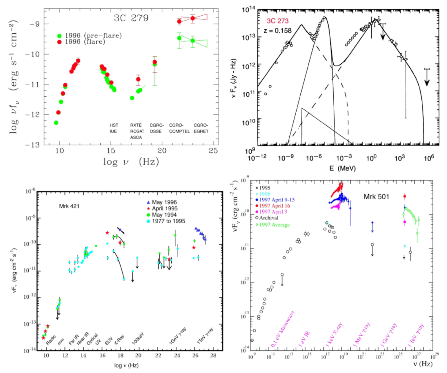
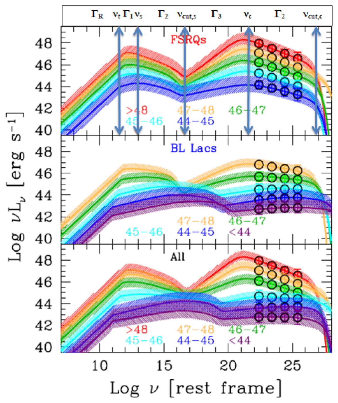
2. Spectral Energy Distribution of Radio Loud AGN
3. The AGN Sample and Spectral Fitting
- po (simple power-law, for the Planck spectra);
- bknpo (broken power-law, for the Planck spectra);
- po*tbabs (absorbed power-law, for the Swift/XRT+BAT spectra);
- bknpo*tbabs (absorbed broken power-law, for the Swift/XRT+BAT spectra).
4. AGN Sample: Interconnection of Radio and X-ray Spectra
5. Conclusions
Author Contributions
Funding
Institutional Review Board Statement
Informed Consent Statement
Data Availability Statement
Acknowledgments
Conflicts of Interest
Appendix A. Planck Spectral Models
- Simple power-law pow;
- Broken power-law bknpo.

| Object | Power-Law | Broken Power-Law | |||||
|---|---|---|---|---|---|---|---|
| Parameter -> | E, 10 eV | P | |||||
| [HB 89] 2142-758 | 1.29 ± 0.05 | 103.4/5 | 0.7 ± 0.2 | 2.0 ± 0.2 | 1.46 ± 0.05 | 6.6/4 | 0.2 % |
| [HB 89] 2230+114 | 1.52 ± 0.05 | 81.4/5 | 1.39 ± 0.04 | 5.7 ± 0.8 | 2.2 ± 0.2 | 5.7/4 | 0.2 % |
| PMN J0623-6436 | 1.38 ± 0.08 | 26.1/4 | 0.87 | 2.1 ± 0.1 | 1.59 ± 0.08 | 4.9/3 | 3.7% |
| PMN J0525-2338 | 1.61 ± 0.12 | 10.8/2 | 0.6 ± 0.6 | 2.5 ± 0.3 | 2.5 ± 0.5 | 1.1/1 | 20.7% |
| PMN J1508-4953 | 0.9 ± 0.2 | 10.8/2 | 0.6 ± 0.5 | 3.5 ± 0.7 | 1.51 ± 0.46 | 1.3/1 | 22.6% |
| 3C 273 | 1.35 ± 0.02 | 4520.6/6 | 0.96 ± 0.01 | 3.8 ± 0.2 | 1.76 ± 0.03 | 16.6/5 | <0.01% |
| 3C 279 | 1.47 ± 0.03 | 43.9/7 | 1.12 ± 0.08 | 4 ± 1 | 1.60 ± 0.03 | 7.9/6 | 0.2% |
| 3C 309.1 | 1.41 ± 0.13 | 0.71/2 | - | - | - | - | - |
| 3C 345 | 1.61 ± 0.03 | 61.6/6 | 1.33 ± 0.06 | 3.8 ± 0.5 | 1.80 ± 0.04 | 3.1/4 | 0.3% |
| 3C 380 | 1.7 ± 0.05 | 24.9/5 | 1.53 ± 0.09 | 3.7 ± 0.5 | 1.95 ± 0.15 | 6.6/4 | 3% |
| 3C 454.3 | 0.95 ± 0.03 | 426.7/7 | 0.31 ± 0.05 | 3.0 ± 0.20 | 1.21 ± 0.03 | 6.2/5 | <0.01% |
| 4C +31.63 | 1.2 ± 0.2 | 20.0/5 | 1.0 ± 0.35 | 3.0 ± 0.9 | 1.49 ± 0.15 | 4.0/3 | 9% |
| 4C +32.14 | 1.62 ± 0.14 | 2.9/3 | - | - | - | - | - |
| 4C +49.22 | 1.29 ± 0.05 | - | - | - | - | - | - |
| 4C +50.11 | 1.60 ± 0.05 | - | - | - | - | - | - |
| 4C +71.078 | 1.33 ± 0.05 | 347.3/5 | 0.73 ± 0.05 | 3.2 ± 0.5 | 1.92 ± 0.05 | 0.8/3 | 0.01% |
| 4C +73.18 | 1.65 ± 0.07 | 9.4/5 | 1.04 ± 0.55 | 2.2 ± 0.7 | 1.75 ± 0.08 | 2.9/3 | 17% |
| 8C 1849+670 | 1.26 ± 0.10 | 24.4/5 | 1.25 ± 0.19 | 3.7 ± 1.5 | 1.53 ± 0.11 | 3.6/3 | 5.6% |
| S5 0212+735 | 1.6 ± 0.6 | 7.0/3 | 1.57 ± 0.08 | 4 ± 0.6 | 2.0 ± 0.3 | 1.9/2 | 14.6% |
| S5 0716+714 | 1.18 ± 0.06 | 22.2/4 | 0.75 ± 0.28 | 3.4 ± 0.6 | 1.28 | 4.3/3 | 3.9% |
| S5 1039+81 | 1.38 ± 0.25 | 1.3/2 | - | - | - | - | - |
| S5 1803+784 | 1.3 ± 0.05 | 32.6/5 | 1.17 ± 0.04 | 4.0 ± 0.8 | 1.51 ± 0.06 | 1.8/3 | 1.3% |
| PKS 0312-770 | 1.45 ± 0.08 | 35.8/4 | 0.4 ± 0.3 | 2.0 ± 0.2 | 1.95 ± 0.15 | 2.7/3 | 0.9% |
| PKS 1127-14 | 1.16 ± 0.08 | 141.9/4 | 0.6 ± 0.4 | 2.9 ± 0.6 | 1.7 ± 0.08 | 0.9/2 | 0.6% |
| PKS 1143-696 | 1.3 ± 0.2 | 17.3/4 | 1.12 ± 0.35 | 3.3 ± 1.5 | 1.85 ± 0.27 | 6.0/3 | 10% |
| PKS 1329-049 | 1.22 ± 0.09 | 7.2/4 | - | - | - | - | - |
| PKS 1335-127 | 1.35 ± 0.03 | 52.1/5 | 1.13 ± 0.04 | 3.5 ± 0.8 | 1.64 ± 0.06 | 4.5/3 | 2.5% |
| PKS 1510-08 | 1.38 ± 0.04 | 65.3/5 | 0.06 | 3.9 ± 0.4 | 1.85 ± 0.09 | 7.4/4 | 0.5% |
| PKS 1622-29 | 1.08 ± 0.08 | 0.9/4 | - | - | - | - | - |
| PKS 1830-21 | 1.74 ± 0.04 | 3.8/4 | - | - | - | - | - |
| PKS 2005-489 | 1.31 ± 0.11 | 14.5/3 | 1.13 ± 0.12 | 5.5 ± 0.9 | 1.9 ± 0.3 | 4.7/2 | 17.8% |
| PKS 2008-159 | 1.64 ± 0.14 | 1.9/1 | - | - | - | - | - |
| PKS 2052-47 | 1.48 ± 0.03 | 10.6/5 | 1.53 ± 0.04 | 4.5 ± 1.5 | 1.41 ± 0.07 | 8.6/4 | 38.9% |
| PKS 2145+06 | 1.57 ± 0.2 | 127.8/5 | 1.35 ± 0.04 | 3.9 ± 0.4 | 1.97 ± 0.05 | 4.4/3 | 0.6% |
| PKS 2149-306 | 1.52 ± 0.09 | 0.42/1 | - | - | - | - | - |
| PKS 2227-088 | 1.22 ± 0.04 | 15.7/4 | 0.97 ± 0.06 | 4.2 ± 0.9 | 1.61 ± 0.08 | 3.2/2 | 20% |
| PKS 2331-240 | 1.22 ± 0.04 | 28.0/3 | 0.9 ± 0.07 | 3.6 ± 0.3 | 1.57 ± 0.12 | 3.9/2 | 7.2% |
| PKS 0402-362 | 1.13 ± 0.02 | 316.3/7 | 0.65 ± 0.07 | 3.1 ± 0.5 | 1.37 ± 0.05 | 20.9/5 | 0.1% |
| PKS 0405-12 | 1.64 ± 0.17 | 1.3/1 | - | - | - | - | - |
| PKS 0426-380 | 1.43 ± 0.06 | 15.9/6 | 0.7 ± 0.4 | 2.0 ± 0.6 | 1.52 ± 0.06 | 7.7/4 | 23% |
| PKS 0521-36 | 1.21 ± 0.02 | 38.1/5 | 1.11 ± 0.03 | 4.1 ± 0.7 | 1.32 ± 0.03 | 5.6/3 | 5.6% |
| PKS 0528+134 | 1.90 ± 0.15 | 4.5/3 | - | - | - | - | - |
| PKS 0537-286 | 2.0 ± 0.4 | 0.5/1 | - | - | - | - | - |
| PKS 0537-441 | 1.33 ± 0.02 | 44.7/7 | 1.10 ± 0.08 | 4.1 ± 0.8 | 1.43 ± 0.03 | 9.2/5 | 1.9% |
| PKS 0723-008 | 1.17 ± 0.04 | 91.7/5 | 0.85 ± 0.06 | 3.7 ± 0.6 | 1.48 ± 0.06 | 3.4/3 | 0.7% |
| B2 0552+39A | 2.0 ± 0.1 | 7.1/3 | 2.5 ± 0.3 | 1.9 ± 0.5 | 1.78 ± 0.10 | 1.2/1 | 41.3% |
| B2 2023+33 | 1.28 ± 0.12 | 13.8/3 | 1.37 ± 0.15 | 7.4 ± 0.8 | −0.2 ± 0.8 | 6.03/2 | 25% |
| B1921-293 | 1.43 ± 0.10 | 509.7/6 | 1.32 ± 0.01 | 4.9 ± 0.3 | 1.72 ± 0.03 | 7.9/4 | 0.02% |
| FBQS J1159+2914 | 1.17 ± 0.06 | 13.4/6 | 1.24 ± 0.19 | unconstr. | 1.15 ± 0.08 | 13.1/5 | 74% |
| II Zw 171 | 1.27 ± 0.16 | 0.03/0 | - | - | - | - | - |
| Mrk 501 | 1.57 ± 0.10 | 2.6/2 | - | - | - | - | - |
| Mrk 1501 | 1.34 ± 0.07 | 8.6/5 | 0.4 ± 0.8 | 1.6 ± 0.4 | 1.47 ± 0.09 | 4.2/4 | 11% |
| NGC 7213 | −1.67 ± 0.15 | 0.59/0 | - | - | - | - | - |
| PG 1222+216 | 1.17 ± 0.08 | 35.2/3 | 0.28 ± 0.22 | 2.4 ± 0.6 | 1.62 ± 0.12 | 1.3/1 | 19% |
| QSO B0309+411 | 1.0 ± 0.2 | 3.9/1 | 0.5 ± 0.6 | 6.0 ± 2.0 | 1.2 ± 0.3 | 0.23/0 | 15.6% |
| QSO B2013+370 | 1.51 ± 0.20 | 0.51/1 | - | - | - | - | - |
Appendix B. X-ray Spectral Models
- Simple power-law with neutral hydrogen absorption pow*tbabs, with the fitting parameters: photon index and absorbing column density ;
- Broken power-law with neutral hydrogen absorption bknpo*tbabs, with the fitting parameters: two photon indices and , break energy and the neutral absorbing column density . The lower fitting values for N were set to the Galactic absorption values for particular object shown in the Table 1, Table 2 and Table 3. In the Table A2 we show the absorption excesses relatively to those values.
| Object | Power-Law | Broken Power-Law | |||||||
|---|---|---|---|---|---|---|---|---|---|
| Parameter -> | N * | E ** | N | P | |||||
| [HB 89] 2142-758 | 1.44 ± 0.07 | <100 | 74/56 | 0.8 ± 0.3 | 1.8 ± 0.3 | 1.49 ± 0.11 | <100 | 68/54 | 10% |
| [HB 89] 2230+114 | 1.41 ± 0.03 | 7 ± 4 | 841/702 | 1.40 ± 0.02 | 7.1 ± 2.1 | 1.96 ± 0.11 | 7 ± 4 | 838/700 | 100% |
| PMN J0623-6436 | 1.63 ± 0.11 | <4 | 85.7/63 | - | - | - | - | - | - |
| 3C 273 | 1.65 ± 0.01 | 3 ± 2 | 1279/829 | 1.52 ± 0.03 | 2.5 ± 0.3 | 1.72 | 3 ± 2 | 1087/827 | <0.01% |
| 3C 279 | 1.59 ± 0.01 | 2 ± 1 | 1165/829 | 1.49 ± 0.05 | 2.5 ± 0.3 | 1.67 ± 0.03 | 2 ± 1 | 1087/827 | <0.01% |
| 3C 309.1 | 1.48 ± 0.07 | <6 | 54.2/65 | - | - | - | - | - | - |
| 3C 345 | 1.64 ± 0.04 | <2 | 258/270 | 1.97 ± 0.22 | 1.2 ± 0.2 | 1.64 ± 0.04 | <2 | 251/268 | 2.5% |
| 3C 380 | 1.89 ± 0.06 | 90 ± 10 | 711/691 | 1.67 ± 0.17 | 2.3 ± 0.9 | 2.1 ± 0.3 | 60 ± 10 | 702/689 | 2% |
| 3C 454.3 | 1.63 ± 0.03 | <4 | 281/270 | 1.92 ± 0.20 | 1.2 ± 0.3 | 1.62 ± 0.03 | <4 | 272/268 | 2% |
| 4C +31.63 | 1.62 ± 0.06 | 80 ± 60 | 118//110 | - | - | - | - | - | - |
| 4C +32.14 | 1.54 ± 0.03 | <20 | 121/112 | 1.47 ± 0.07 | 25 ± 4 | 1.8 ± 0.3 | <20 | 114/110 | 3.8% |
| 4C +49.22 | 1.78 ± 0.02 | <10 | 219/144 | 1.68 ± 0.05 | 5.4 ± 2.8 | 1.84 ± 0.04 | <10 | 202/142 | 0.3% |
| 4C +50.11 | 1.66 | <110 | 76.1/86 | - | - | - | - | - | - |
| 4C +71.078 | 1.49 ± 0.01 | 39 ± 4 | 957/498 | 1.33 ± 0.03 | 6.7 ± 1.8 | 1.73 ± 0.07 | <42 | 602/496 | <0.01% |
| 4C +73.18 | 1.76 ± 0.05 | <5 | 92.4/90 | - | - | - | - | - | - |
| 8C 1849+670 | 1.57 ± 0.03 | <50 | 62.1/42 | 1.72 ± 0.10 | 6.3 ± 5.3 | 1.49 ± 0.11 | <50 | 54.2/40 | 6.6% |
| S5 0212+735 | 1.41 ± 0.08 | 170 ± 100 | 85.5/73 | - | - | - | - | - | - |
| PKS 0312-770 | 1.81 ± 0.03 | <20 | 862/561 | 2.15 ± 0.08 | 2.7 ± 0.3 | 1.41 ± 0.09 | <20 | 659/559 | <0.01% |
| PKS 1127-14 | 1.59 ± 0.05 | 85 ± 16 | 140/111 | 1.49 ± 0.06 | 18.4 ± 9.9 | 2.7 ± 1.6 | 85 ± 16 | 113/109 | <0.01% |
| PKS 1143-696 | 1.72 ± 0.06 | <7 | 64.3/68 | 2.5 ± 1.4 | unc. | 1.79 ± 0.14 | <7 | 62.8/66 | 41% |
| PKS 1329-049 | 1.38 ± 0.08 | <55 | 34.3/32 | 1.33 ± 0.09 | unc. | unc. | <40 | 32.0/30 | 35% |
| PKS 1335-127 | 1.47 ± 0.02 | <2 | 759/619 | 1.42 ± 0.02 | 6.4 ± 0.7 | 2.1 ± 0.3 | <2 | 646/617 | <0.01% |
| PKS 1510-08 | 0.02 | <5 | 666/579 | 1.31 ± 0.02 | 10.7 ± 6.5 | 1.39 ± 0.05 | <5 | 661/577 | 8.8% |
| PKS 1622-29 | 1.44 ± 0.02 | <2 | 748/619 | 1.39 ± 0.03 | 7.1 ± 0.9 | 1.91 | <2 | 659/617 | <0.01% |
| PKS 1830-21 | 1.33 ± 0.02 | <2 | 769.6/619 | 1.40 ± 0.03 | 5.3 ± 0.7 | 1.21 ± 0.05 | <2 | 689/617 | <0.01% |
| PKS 2005-489 | 1.54 ± 0.02 | 19 ± 4 | 993/619 | 1.42 ± 0.02 | 7.1 ± 0.6 | 2.4 ± 0.3 | 6 ± 1 | 654/617 | <0.01% |
| PKS 2008-159 | 1.42 ± 0.02 | <3 | 745/695 | 1.40 ± 0.02 | 6.4 ± 0.9 | 2.0 | <3 | 730/693 | <0.01% |
| PKS 2052-47 | 1.39 ± 0.02 | 25 ± 4 | 751/695 | 1.38 ± 0.02 | 11 ± 4 | 2.2 | 25 ± 4 | 737/693 | 0.2% |
| PKS 2145+06 | 1.39 ± 0.02 | <6 | 744/695 | 1.28 ± 0.06 | 2.0 ± 0.5 | 1.43 ± 0.04 | <6 | 730/693 | <0.01% |
| PKS 2149-306 | 1.35 ± 0.01 | 9 ± 7 | 370/255 | 1.22 ± 0.03 | 13.6 ± 4.3 | 1.61 ± 0.13 | 9 ± 7 | 285/253 | <0.01% |
| PKS 2227-088 | 1.46 ± 0.08 | <14 | 43.1/37 | 1.33 ± 1.50 | <85 | 1.69 ± 0.32 | <14 | 40.2/35 | 29.6% |
| PKS 2331-240 | 1.73 ± 0.03 | 14 ± 5 | 384/293 | 1.64 ± 0.04 | 7.6 ± 2.2 | 2.4 ± 0.3 | 14 ± 5 | 298/291 | <0.01% |
| PKS 0402-362 | 1.64 ± 0.04 | 34 ± 10 | 205/168 | 1.58 ± 0.04 | 9.5 ± 9.3 | 2.0 ± 0.5 | 24 ± 10 | 187/166 | <0.01% |
| PKS 0405-12 | 2.5 ± 0.1 | <40 | 94.4/38 | 1.79 ± 0.15 | 21 ± 4 | 2.7 ± 0.3 | <40 | 54.2/36 | <0.01% |
| PKS 0426-380 | 1.43 ± 0.05 | <31 | 93/40 | 1.66 ± 0.07 | 4.1 ± 1.9 | 1.35 ± 0.07 | <31 | 61.8/38 | 0.03% |
| PKS 0521-36 | 1.70 ± 0.02 | <9 | 434/318 | 1.58 ± 0.03 | 4.8 ± 1.8 | 1.86 ± 0.06 | <9 | 357/316 | <0.01% |
| PKS 0528+134 | 1.53 ± 0.06 | 430 ± 90 | 171/146 | 0.93 ± 0.28 | 1.5 | 1.49 ± 0.07 | 340 ± 40 | 168/144 | 28% |
| PKS 0537-286 | 1.29 ± 0.01 | 15 ± 14 | 124/86 | 1.20 ± 0.06 | 10.9 ± 5.2 | 1.36 ± 0.04 | 15 ± 14 | 107/84 | 0.2% |
| PKS 0537-441 | 1.66 ± 0.02 | <5 | 306/292 | 2.0 ± 0.2 | 0.9 ± 0.2 | 1.68 ± 0.03 | <3 | 297/290 | 1.3% |
| PKS 0723-008 | 1.62 ± 0.05 | <3 | 79.6/90 | - | - | - | - | - | - |
| B2 0552+39A | 1.45 ± 0.11 | 26 ± 17 | 20.1/20 | - | - | - | - | - | - |
| S5 0716+714 | 2.22 ± 0.15 | 20 ± 5 | 1731/848 | 2.61 ± 0.09 | 1.24 ± 0.05 | 2.17 ± 0.02 | 20 ± 5 | 1343/846 | <0.01% |
| S5 1039+81 | 1.55 ± 0.07 | <12 | 50.5/29 | 1.25 ± 0.35 | 2.7 ± 1.8 | 1.65 ± 0.12 | <12 | 44.4/27 | 17.6% |
| S5 1803+784 | 1.52 ± 0.04 | <5 | 123/131 | - | - | - | - | - | - |
| B1921-293 | 1.82 ± 0.10 | <4 | 53.6/73 | - | - | - | - | - | - |
| B2 2023+33 | 1.46 ± 0.17 | <250 | 8.7/9 | - | - | - | - | - | - |
| FBQS J1159+2914 | 1.54 ± 0.04 | <13 | 218/206 | 1.53 ± 0.04 | 47 | >1.6 | <11 | 214/204 | 15.1% |
| II Zw 171 | 1.81 ± 0.05 | <7 | 146/136 | 2.1 ± 1.0 | unc. | 1.82 ± 0.09 | <7 | 144/134 | 40% |
| Mrk 501 | 2.10 ± 0.01 | <1 | 652/457 | 2.04 ± 0.01 | 56 ± 25 | 2.7 ± 0.5 | <1 | 642/455 | 7.2% |
| Mrk 1501 | 1.63 ± 0.03 | <6 | 172/128 | 1.62 ± 0.04 | 74 ± 69 | 2.91 ± 0.16 | <6 | 169/126 | 33% |
| NGC 7213 | 1.69 ± 0.03 | 14 ± 13 | 72.2/94 | - | - | - | - | - | - |
| PG 1222+216 | 1.41 ± 0.03 | <11 | 739/277 | 2.16 ± 0.17 | 1.1 ± 0.1 | 1.43 ± 0.03 | <11 | 285/275 | <0.01% |
| PMN J0525-2338 | 1.5 ± 0.8 | <95 | 7.2/5 | - | - | - | - | - | - |
| PMN J1508-4953 | 1.32 ± 0.07 | <300 | 30.3/23 | >1.0 | 0.9 ± 0.2 | 1.30 ± 0.06 | 20 ± 10 | 19/21 | 0.7% |
| QSO B0309+411 | 1.79 ± 0.04 | <60 | 158.9/128 | 2.7 ± 0.6 | 1.2 ± 0.1 | 1.80 ± 0.07 | <60 | 151.4/126 | 4.8% |
| QSO B2013+370 | 1.57 ± 0.08 | 56 ± 25 | 75.3/54 | 1.6 ± 0.2 | 22 ± 18 | 2.2 ± 0.8 | 59 ± 25 | 65.3/52 | 2.5% |
| 1 | https://swift.gsfc.nasa.gov/results/bs105mon/ Accessed on 10 June 2020. |
| 2 | https://simbad.u-strasbg.fr/simbad/ Accessed on 10 June 2020. |
| 3 | https://www.isdc.unige.ch/heavens Accessed on 12 June 2020. |
| 4 | https://www.swift.ac.uk/ Accessed on 12 June 2020. |
| 5 | https://swift.gsfc.nasa.gov/results/bs105mon/ Accessed on 10 June 2020. |
| 6 | https://heasarc.gsfc.nasa.gov/lheasoft/ Accessed on 15 July 2020. |
References
- Padovani, P.; Giommi, P. A sample-oriented catalogue of BL Lacertae objects. MNRAS 1995, 277, 1477–1490. [Google Scholar] [CrossRef]
- Abdo, A.A.; Ackermann, M.; Agudo, I.; Ajello, M.; Aller, H.D.; Aller, M.F.; Angelakis, E.; Arkharov, A.A.; Axelsson, M.; Bach, U.; et al. The Spectral Energy Distribution of Fermi Bright Blazars. ApJ 2010, 716, 30–70. [Google Scholar] [CrossRef]
- Giommi, P.; Polenta, G.; Lähteenmäki, A.; Thompson, D.J.; Capalbi, M.; Cutini, S.; Gasparrini, D.; González-Nuevo, J.; León-Tavares, J.; López-Caniego, M.; et al. Simultaneous Planck, Swift, and Fermi observations of X-ray and γ-ray selected blazars. Astron. Astrophys. 2012, 541, A160. [Google Scholar] [CrossRef]
- Ghisellini, G.; Righi, C.; Costamante, L.; Tavecchio, F. The Fermi blazar sequence. MNRAS 2017, 469, 255–266. [Google Scholar] [CrossRef]
- Pei, Z.; Fan, J.; Yang, J.; Huang, D.; Li, Z. The Estimation of Fundamental Physics Parameters for Fermi-LAT Blazars. arXiv 2021, arXiv:2112.00530. [Google Scholar]
- Grandi, P.; Palumbo, G.G.C. Jet and Accretion-Disk Emission Untangled in 3C 273. Science 2004, 306, 998–1002. [Google Scholar] [CrossRef][Green Version]
- Fedorova, E.; Hnatyk, B.I.; Zhdanov, V.I.; Del Popolo, A. X-ray Properties of 3C 111: Separation of Primary Nuclear Emission and Jet Continuum. Universe 2020, 6, 219. [Google Scholar] [CrossRef]
- Zhu, S.F.; Brandt, W.N.; Luo, B.; Wu, J.; Xue, Y.Q.; Yang, G. The LX-Luv-Lradio relation and corona-disc-jet connection in optically selected radio-loud quasars. MNRAS 2020, 496, 245–268. [Google Scholar] [CrossRef]
- Gao, H.; Lei, W.H.; Wu, X.F.; Zhang, B. Compton scattering of self-absorbed synchrotron emission. MNRAS 2013, 435, 2520–2531. [Google Scholar] [CrossRef]
- Planck Collaboration; Lawrence, C.R. The Planck Early Release Compact Source Catalog. In Proceedings of the American Astronomical Society Meeting Abstracts #217, Seattle, WA, USA, 9–13 January 2011; 217, p. 243.07. Available online: https://www.isdc.unige.ch/heavens/ (accessed on 15 July 2020).
- La Mura, G.; Busetto, G.; Ciroi, S.; Rafanelli, P.; Berton, M.; Congiu, E.; Cracco, V.; Frezzato, M. Relativistic plasmas in AGN jets. From synchrotron radiation to γ-ray emission. Eur. Phys. J. D 2017, 71, 95. [Google Scholar] [CrossRef]
- Urry, C.M. Multiwavelength properties of blazars. Adv. Space Res. 1998, 21, 89–100. [Google Scholar] [CrossRef]
- Willingale, R.; Starling, R.L.C.; Beardmore, A.P.; Tanvir, N.R.; O’Brien, P.T. Calibration of X-ray absorption in our Galaxy. MNRAS 2013, 431, 394–404. [Google Scholar] [CrossRef]
- Anjum, M.S.; Tammi, J. Nonlinear synchrotron self-compton modelling of blazars. In Proceedings of the 2015 Fourth International Conference on Aerospace Science and Engineering (ICASE), Islamabad, Pakistan, 2–4 September 2015; pp. 1–8. [Google Scholar] [CrossRef]
- Cutini, S.; Ciprini, S.; Orienti, M.; Tramacere, A.; D’Ammando, F.; Verrecchia, F.; Polenta, G.; Carrasco, L.; D’Elia, V.; Giommi, P.; et al. Radio-gamma-ray connection and spectral evolution in 4C +49.22 (S4 1150+49): The Fermi, Swift and Planck view. MNRAS 2014, 445, 4316–4334. [Google Scholar] [CrossRef]
- Nair, S.; Narasimha, D.; Rao, A.P. PKS 1830-211 as a Gravitationally Lensed System. ApJ 1993, 407, 46. [Google Scholar] [CrossRef]
- D’Ammando, F.; Orienti, M.; Tavecchio, F.; Ghisellini, G.; Torresi, E.; Giroletti, M.; Raiteri, C.M.; Grandi, P.; Aller, M.; Aller, H.; et al. Unveiling the nature of the γ-ray emitting active galactic nucleus PKS 0521-36. MNRAS 2015, 450, 3975–3990. [Google Scholar] [CrossRef]


| Object | Type | RA [h, m, s] | Dec [o, , ] | z | [cm] |
|---|---|---|---|---|---|
| PKS 0426-380 | LSP | 04 28 40.42 | −37 56 19.58 | 1.11 | |
| PKS 0521-36 | LSP | 05 22 57.98 | −36 27 30.84 | 0.05 | |
| PKS 0537-441 | LSP | 05 38 50.36 | −44 05 08.93 | 0.89 | |
| S5 0716+714 | ISP | 07 21 53.44 | +71 20 36.36 | 0.3 | |
| Mrk 501 | HSP | 16 53 52.21 | +39 45 36.6 | 0.03 | |
| S5 1803+784 | LSP | 18 00 45.68 | +78 28 04.01 | 0.68 | |
| PKS 2005-489 | HSP | 20 09 25.39 | −48 49 53.72 | 0.07 | |
| PKS 2331-240 | ISP | 23 33 55.23 | −23 43 40.65 | 0.05 |
| Object | Type | RA [h, m, s] | Dec [o, , ] | z | [cm] |
|---|---|---|---|---|---|
| S5 0212+735 | FSRQ-LSP | 02 17 30.81 | +73 49 32.61 | 2.36 | |
| PKS 0312-770 | FSRQ | 03 11 55.25 | −76 51 50.84 | 0.22 | |
| 4C +32.14 | FSRQ | 03 36 30.1 | +32 18 29.34 | 1.26 | |
| 4C +50.11 | FSRQ | 03 59 29.74 | +50 57 50.16 | 1.52 | |
| PKS 0402-362 | FSRQ | 04 03 53.74 | −36 05 01.91 | 1.42 | |
| PMN J0525-2338 | FSRQ | 05 25 06.50 | −23 38 10.8 | 3.1 | |
| PKS 0528+134 | FSRQ-LSP | 05 30 56.46 | +13 31 55.14 | 2.07 | |
| PKS 0537-286 | FSRQ | 05 39 54.28 | −28 39 55.94 | 3.1 | |
| B2 0552+39A | FSRQ | 05 55 30.80 | +39 48 49.16 | 2.37 | |
| PMN J0623-6436 | FSRQ | 06 23 07.69 | −64 36 20.71 | 0.12 | |
| PKS 0723-008 | FSRQ | 07 25 50.63 | -00 54 56.54 | 0.12 | |
| 4C +71.078 | FSRQ | 08 41 24.35 | +70 53 42.28 | 2.21 | |
| S5 1039+81 | FSRQ | 10 44 23.06 | +80 54 39.44 | 1.26 | |
| PKS 1127-14 | FSRQ-LSP | 11 30 07.05 | −14 49 27.38 | 1.18 | |
| 4C +49.22 | FSRQ-LSP | 11 53 24.46 | +49 31 08.83 | 0.33 | |
| FBQS J1159+2914 | FSRQ-LSP | 11 59 31.83 | +29 14 43.82 | 0.72 | |
| PG 1222+216 | FSRQ | 12 24 54.45 | +21 22 46.38 | 0.43 | |
| 3C 273 | FSRQ-LSP | 12 29 06.69 | +02 03 08.59 | 0.15 | |
| 3C 279 | FSRQ-LSP | 12 56 11.16 | −05 47 21.53 | 0.53 | |
| PKS 1329-049 | FSRQ | 13 32 04.46 | −05 09 43.3 | 2.15 | |
| PKS 1335-127 | FSRQ | 13 37 39.78 | −12 57 24.69 | 0.54 | |
| PMN J1508-4953 | FSRQ | 15 08 38.94 | −49 53 02.32 | - | |
| PKS 1510-08 | FSRQ | 15 12 50.53 | −09 05 59.82 | 0.36 | |
| PKS 1622-29 | FSRQ | 16 26 06 | −29 51 26.97 | 0.81 | |
| 3C 345 | FSRQ-LSP | 16 42 58.81 | +39 48 36.99 | 0.59 | |
| PKS 1830-21 | FSRQ-LSP | 18 33 39.92 | −21 03 39 | 2.5 | |
| B1921-293 | FSRQ | 19 24 51.05 | −29 14 30.12 | 0.35 | |
| 4C +73.18 | FSRQ | 19 27 48.49 | +73 58 01.57 | 0.3 | |
| PKS 2008-159 | FSRQ | 20 11 15.71 | −15 46 40.25 | 1.18 | |
| QSO B2013+370 | FSRQ | 20 15 28.72 | +37 10 59.51 | 0.85 | |
| B2 2023+33 | FSRQ | 20 25 10.84 | +33 43 | 0.22 | |
| PKS 2052-47 | FSRQ | 20 56 16.35 | −47 14 47.62 | 1.49 | |
| [HB 89] 2142-758 | FSRQ | 21 48 | −75.575 | 1.13 | |
| PKS 2145+06 | FSRQ | 21 48 05.45 | +06 57 38.6 | 1 | |
| PKS 2149-306 | FSRQ-LSP | 21 51 55.52 | −30 27 53.69 | 2.35 | |
| 4C +31.63 | FSRQ-LSP | 22 03 14.97 | +31 45 38.26 | 0.29 | |
| II Zw 171 | FSRQ | 22 11 53.88 | +18 41 49.85 | 0.06 | |
| [HB 89] 2230+114 | FSRQ | 22 31 48 | +11.721 | 1.03 | |
| PKS 2227-088 | FSRQ-LSP | 22 29 40.08 | −08 32 54.43 | 1.55 | |
| 3C 454.3 | FSRQ | 22 53 57 | +16 08 53 | 0.85 | |
| Object | Type | RA [h, m, s] | Dec [o, , ] | z | [cm] |
|---|---|---|---|---|---|
| Mrk 1501 | Seyfert 1 | 00 10 31.00 | +10 58 29.5 | 0.09 | |
| QSO B0309+411 | Seyfert 1 | 03 13 01.96 | +41 20 01.18 | 0.13 | |
| PKS 0405-12 | Seyfert 1 | 04 07 48.43 | −12 11 36.66 | 0.57 | |
| PKS 1143-696 | Seyfert 1 | 11 45 53.62 | −69 54 01.79 | 0.24 | |
| 3C 309.1 | Seyfert 1 | 14 59 07.58 | +71 40 19.86 | 0.9 | |
| 3C 380 | Seyfert 1 | 18 29 31.78 | +48 44 46.15 | 0.69 | |
| 8C 1849+670 | Seyfert 1 | 18 49 16.07 | +67 05 41.68 | 0.66 | |
| NGC 7213 | Seyfert 1 | 22 09 16.21 | −47 10 00.08 | 0.005 |
| Object | Radio | X-rays | ||||
|---|---|---|---|---|---|---|
| Parameter -> | E, 10 eV | E, keV | ||||
| Mrk 1501 | 0.4 ± 0.8 | 1.6 ± 0.4 | 1.47 ± 0.09 | 1.62 ± 0.03 | 74 ± 69 | 2.91 ± 0.16 |
| S5 0212+735 | 1.57 ± 0.08 | 4.0 ± 0.6 | 2.0 ± 0.3 | 1.41 ± 0.08 | - | - |
| PKS 0312-770 | 0.4 ± 0.3 | 2.0 ± 0.2 | 1.95 ± 0.15 | 2.15 ± 0.08 | 2.7 ± 0.3 | 1.41 ± 0.09 |
| QSO B0309+411 | 1.0 ± 0.2 | - | - | 2.7 ± 0.6 | 1.2 ± 0.2 | 1.8 ± 0.07 |
| 4C +32.14 | 1.62 ± 0.14 | - | - | 1.47 ± 0.07 | 25 ± 4 | 1.8 ± 0.3 |
| 4C +50.11 | 1.60 ± 0.05 | - | - | 1.66 | - | - |
| PKS 0402-362 | 1.13 ± 0.08 | 6.0 ± 0.6 | 1.45 ± 0.05 | 1.58 ± 0.04 | 9.5 ± 9.3 | 2.0 ± 0.5 |
| PKS 0405-12 | 1.64 ± 0.09 | - | - | 1.79 ± 0.15 | 21 ± 4 | 2.7 ± 0.3 |
| PKS 0426-380 | 0.7 ± 0.4 | 2.0 ± 0.6 | 1.57 ± 0.08 | 1.66 ± 0.07 | 4.1 ± 1.9 | 1.35 ± 0.07 |
| PKS 0521-36 | 1.11 ± 0.09 | 4.1 ± 0.7 | 1.32 ± 0.03 | 1.58 ± 0.03 | 4.8 ± 1.8 | 1.86 ± 0.06 |
| PMN J0525-2338 | 0.6 ± 0.6 | 2.5 ± 0.3 | 2.5 ± 0.5 | 1.5 ± 0.8 | - | - |
| PKS 0528+134 | 1.9 ± 0.1 | - | - | 0.9 ± 0.3 | 1.5 ± 0.9 | 1.49 ± 0.07 |
| PKS 0537-441 | 2.0 ± 0.4 | - | - | 2.0 ± 0.2 | 0.9 ± 0.2 | 1.68 ± 0.03 |
| PKS 0537-286 | 1.10 ± 0.08 | 4.1 ± 0.8 | 1.43 ± 0.03 | 1.20 ± 0.06 | 10.9 ± 5.2 | 1.36 ± 0.04 |
| B2 0552+39A | 2.5 ± 0.3 | 1.9 ± 0.5 | 1.78 ± 0.10 | 1.45 ± 0.11 | - | - |
| PMN J0623-6436 | 0.87 | 2.1 ± 0.1 | 1.59 ± 0.08 | 1.63 ± 0.11 | - | - |
| S5 0716+714 | 0.75 ± 0.29 | 3.4 ± 0.6 | 1.28 ± 0.07 | 2.02 ± 0.09 | 6.1 ± 0.4 | 1.13 ± 0.06 |
| PKS 0723-008 | 0.85 ± 0.06 | 3.7 ± 0.6 | 1.48 ± 0.06 | 1.62 ± 0.05 | - | - |
| S5 1039+81 | 1.38 ± 0.15 | - | - | 1.25 ± 0.35 | 2.7 ± 1.8 | 1.65 ± 0.12 |
| PKS 1127-14 | 0.6 ± 0.4 | 2.9 ± 0.6 | 1.70 ± 0.08 | 1.49 ± 0.06 | 18.4 ± 9.9 | 2.7 ± 1.6 |
| PKS 1143-696 | 1.12 ± 0.35 | 3.3 ± 1.5 | 1.85 ± 0.27 | 2.5 ± 1.4 | unc. | 1.79 ± 0.14 |
| 4C +49.22 | 1.29 ± 0.05 | - | - | 1.68 ± 0.05 | 5.4 ± 2.8 | 1.84 ± 0.04 |
| FBQS J1159+2914 | 1.17 ± 0.06 | - | - | 1.53 ± 0.04 | 47 | >1.6 |
| PG 1222+216 | 0.28 ± 0.22 | 2.4 ± 0.6 | 1.62 ± 0.12 | 2.16 ± 0.17 | 1.1 ± 0.1 | 1.43 ± 0.03 |
| 3C 273 | 0.96 ± 0.01 | 3.8 ± 0.2 | 1.76 ± 0.03 | 1.52 ± 0.03 | 2.5 ± 0.3 | 1.72 |
| 3C 279 | 1.12 ± 0.08 | 4 ± 1 | 1.60 ± 0.03 | 1.49 ± 0.05 | 2.5 ± 0.3 | 1.67 ± 0.03 |
| PKS 1329-049 | 1.22 ± 0.09 | - | - | 1.33 ± 0.09 | - | - |
| PKS 1335-127 | 1.13 ± 0.04 | 3.5 ± 0.8 | 1.64 ± 0.06 | 1.42 ± 0.02 | 6.4 ± 0.7 | 2.1 ± 0.3 |
| 3C 309.1 | 1.41 ± 0.13 | - | - | 1.48 ± 0.07 | - | - |
| PMN J1508-4953 | 0.6 ± 0.5 | 3.5 ± 0.7 | 1.5 ± 0.3 | 1.32 ± 0.07 | - | - |
| PKS 1510-08 | 3.3 ± 0.4 | 1.85 ± 0.09 | 1.31 ± 0.02 | 10.7 ± 6.5 | 1.39 ± 0.05 | |
| PKS 1622-29 | 1.08 ± 0.08 | - | - | 1.39 ± 0.03 | 7.1 ± 0.9 | 1.91 |
| 3C 345 | 1.33 ± 0.02 | 3.8 ± 0.8 | 1.80 ± 0.04 | 1.97 ± 0.22 | 1.2 ± 0.2 | 1.64 ± 0.04 |
| Mrk 501 | 1.57 ± 0.10 | - | - | 2.09 ± 0.01 | 21 ± 14 | 2.46 ± 0.13 |
| S5 1803+784 | 1.17 ± 0.04 | 4.0 ± 0.8 | 1.51 ± 0.06 | 1.52 ± 0.04 | - | - |
| 3C 380 | 1.53 ± 0.09 | 3.7 ± 0.5 | 1.95 ± 0.15 | 1.67 ± 0.17 | 2.3 ± 0.9 | 2.1 ± 0.3 |
| PKS 1830-21 | 1.74 ± 0.04 | - | - | 1.40 ± 0.03 | 5.3 ± 0.7 | 1.21 ± 0.05 |
| 8C 1849+670 | 1.26 ± 0.19 | 3.7 ± 1.6 | 1.53 ± 0.11 | 1.72 ± 0.10 | 6.3 ± 5.3 | 1.49 ± 0.1 |
| B1921-293 | 1.32 ± 0.01 | 4.9 ± 0.3 | 1.72 ± 0.03 | 1.82 ± 0.10 | - | - |
| 4C +73.18 | 1.04 ± 0.55 | 2.2 ± 0.7 | 1.75 ± 0.08 | 1.76 ± 0.05 | - | - |
| PKS 2005-489 | 1.13 ± 0.12 | 5.5 ± 0.9 | 1.9 ± 0.3 | 1.42 ± 0.02 | 7.1 ± 0.6 | 2.4 ± 0.3 |
| PKS 2008-159 | 1.64 ± 0.14 | - | - | 1.40 ± 0.02 | 6.4 ± 0.9 | 2.0 |
| QSO B2013+370 | 1.51 ± 0.20 | - | - | 1.16 ± 0.20 | 22 ± 18 | 2.2 ± 0.8 |
| PKS 2052-47 | 1.39 ± 0.04 | 4.5 ± 1.5 | 1.41 ± 0.07 | 1.38 ± 0.02 | 11.0 ± 0.4 | 2.2 |
| PKS 2145+06 | 1.35 ± 0.04 | 3.9 ± 0.4 | 1.97 ± 0.05 | 1.28 ± 0.06 | 2.0 ± 0.5 | 1.43 ± 0.01 |
| [HB 89] 2142-758 | 0.7 ± 0.2 | 2.0 ± 0.2 | 1.46 ± 0.05 | 0.8 ± 0.3 | 1.8 ± 0.3 | 1.49 ± 0.11 |
| 4C +31.63 | 1.0 ± 0.4 | 3.0 ± 0.9 | 1.49 ± 0.154 | 1.62 ± 0.06 | - | - |
| II Zw 171 | 1.27 ± 0.16 | - | - | 1.81 ± 0.05 | - | - |
| PKS 2149-306 | 1.12 ± 0.09 | - | - | 1.22 ± 0.03 | 14 ± 5 | 1.61 ± 0.13 |
| NGC 7213 | −1.67 ± 0.15 | - | - | 1.69 ± 0.03 | - | - |
| PKS 2227-088 | 0.97 ± 0.06 | 4.2 ± 0.9 | 1.61 ± 0.08 | 1.3 ± 1.5 | <85 | 1.69 ± 0.32 |
| [HB 89] 2230+114 | 1.39 ± 0.04 | 5.7 ± 0.8 | 2.0 ± 0.2 | 1.40 ± 0.02 | 7.1 ± 2.1 | 1.96 ± 0.11 |
| 3C 454.3 | 0.37 ± 0.05 | 3.0 ± 0.2 | 1.21 ± 0.03 | 1.92 ± 0.20 | 1.2 ± 0.3 | 1.62 ± 0.03 |
| PKS 2331-240 | 0.9 ± 0.07 | 3.6 ± 0.3 | 1.57 ± 0.12 | 1.64 ± 0.04 | 7.6 ± 2.2 | 2.4 ± 0.3 |
| 4C +71.078 | 0.73 ± 0.05 | 3.2 ± 0.5 | 1.20 ± 0.15 | 1.33 ± 0.03 | 6.7 ± 1.8 | 1.73 ± 0.07 |
| B2 2023+33 | 1.37 ± 0.15 | 7.4 ± 0.8 | -0.2 ± 0.8 | 1.46 ± 0.17 | - | - |
Publisher’s Note: MDPI stays neutral with regard to jurisdictional claims in published maps and institutional affiliations. |
© 2022 by the authors. Licensee MDPI, Basel, Switzerland. This article is an open access article distributed under the terms and conditions of the Creative Commons Attribution (CC BY) license (https://creativecommons.org/licenses/by/4.0/).
Share and Cite
Fedorova, E.; Hnatyk, B.; Del Popolo, A.; Vasylenko, A.; Voitsekhovskyi, V. Non-Thermal Emission from Radio-Loud AGN Jets: Radio vs. X-rays. Galaxies 2022, 10, 6. https://doi.org/10.3390/galaxies10010006
Fedorova E, Hnatyk B, Del Popolo A, Vasylenko A, Voitsekhovskyi V. Non-Thermal Emission from Radio-Loud AGN Jets: Radio vs. X-rays. Galaxies. 2022; 10(1):6. https://doi.org/10.3390/galaxies10010006
Chicago/Turabian StyleFedorova, Elena, Bohdan Hnatyk, Antonino Del Popolo, Anatoliy Vasylenko, and Vadym Voitsekhovskyi. 2022. "Non-Thermal Emission from Radio-Loud AGN Jets: Radio vs. X-rays" Galaxies 10, no. 1: 6. https://doi.org/10.3390/galaxies10010006
APA StyleFedorova, E., Hnatyk, B., Del Popolo, A., Vasylenko, A., & Voitsekhovskyi, V. (2022). Non-Thermal Emission from Radio-Loud AGN Jets: Radio vs. X-rays. Galaxies, 10(1), 6. https://doi.org/10.3390/galaxies10010006