
Machine and Deep Learning Models for Hypoxemia Severity Triage in CBRNE Emergencies

 , and
, and
Abstract
1. Introduction
2. Materials and Methods
2.1. Data Sources and Libraries
- Data Sources
- Libraries and Tools Utilized
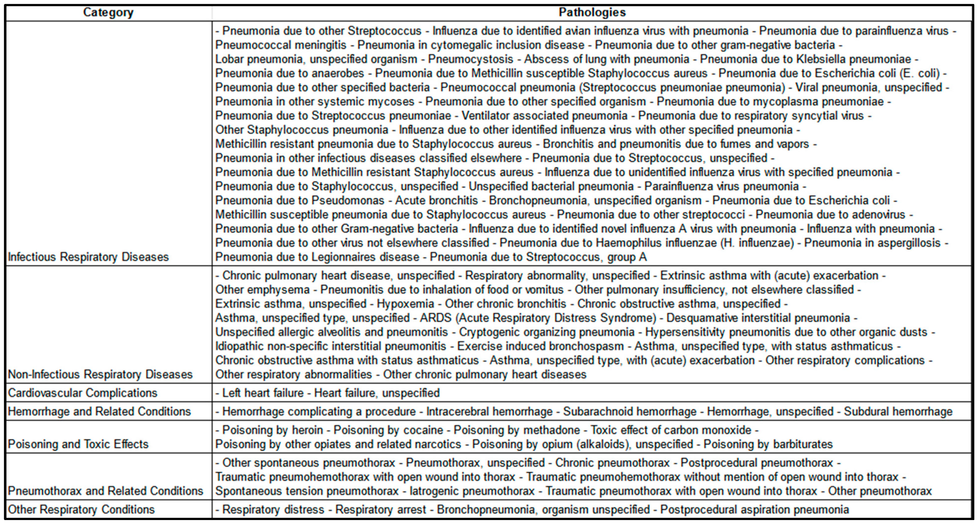
2.2. Inclusion Criteria and Data Representativeness
2.3. Data Preprocessing
2.3.1. Labeling and Feature Engineering
2.3.2. Handling Missing Data and Masks
2.3.3. Prediction Window
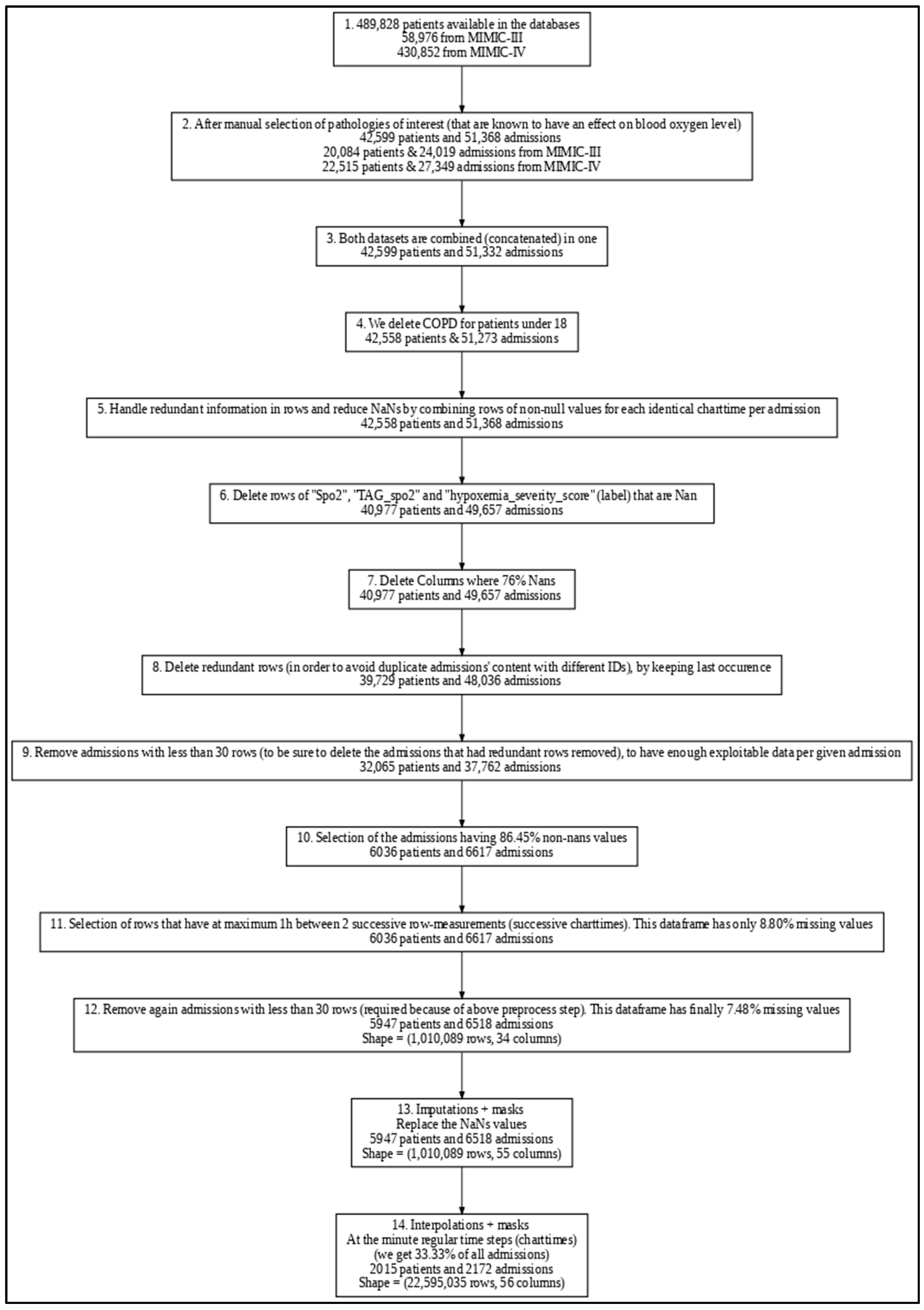
2.3.4. Data Cleaning and Transformation
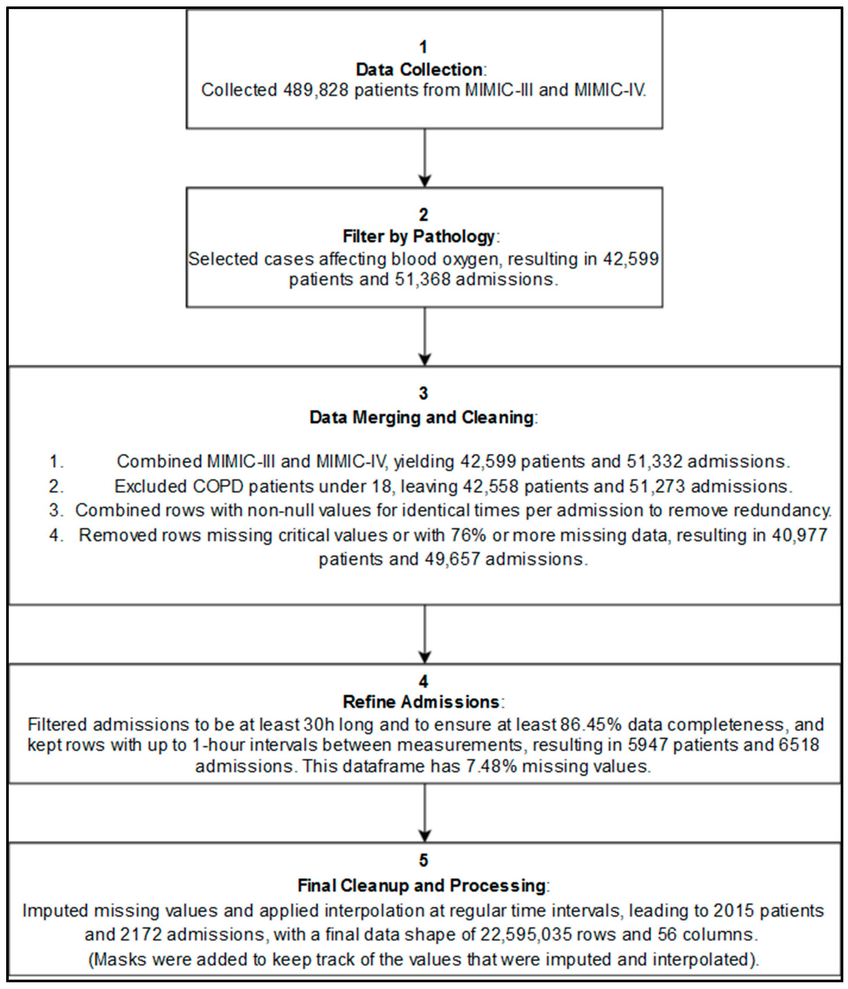
- Duplicated Rows and Admissions Removal: To address potential redundant rows introduced during preprocessing, we merged rows with non-null values recorded at the same charttime (i.e., the same timestamp) within each admission. For eventual duplicate admissions across the combined MIMIC III and IV datasets (which may have different admission IDs), only the most recent occurrence of each redundant row (considering all physiological and demographic features) was retained, while earlier rows were removed to maintain data consistency. This approach ensures that, for each potentially redundant admission, only a single, complete version remains in the final dataset, effectively eliminating duplicate admissions on a row-by-row basis.
- Outlier Handling: Implausible physiological measurements were replaced with NaN and subsequently imputed to address potential human errors in the electronic health records. Specifically, for six key vital signs variables, we excluded values outside defined ranges: respiratory rate, heart rate, and both systolic and diastolic blood pressure above 300 or below 0; SpO2 above 100 or below 0; and temperature readings above 60 or below 0. To ensure consistency, this step was applied both before and after imputation and interpolation.
- Data Rounding: Physiological values were rounded in order to standardize precision, which supports model generalization and may reduce the likelihood of overfitting, especially as future work integrates data from additional hospitals.
- Missing values: Imputation by Chained Equations (MICE) using Histogram-based Gradient Boosting was carried out to complete the 7.48% missing values from our preprocessed dataframe
- Time Alignment: Interpolated data at minute-level intervals to standardize time steps across admissions (synthetic data).
2.3.5. Data Splitting
2.4. Exploratory Data Analysis (EDA)
- Additionally, we performed Exploratory Data Analysis (EDA) to examine data distributions and uncover correlations. Demographics and features: Table 4 illustrates the patients’ age, gender, race, and ethnicity distributions.
- Concerning the demographics, for the races and ethnicities, we referred to the United States Census Bureau [49].
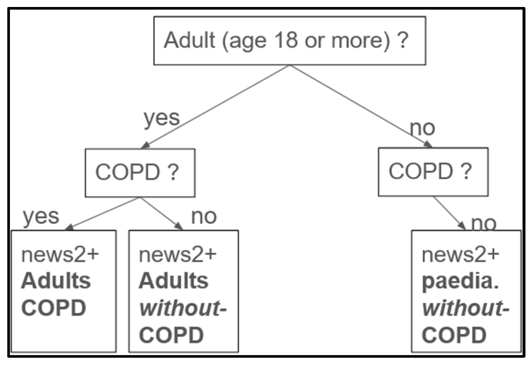
- Label Distribution: We observed an unbalanced dataset, where higher severity scores occur less frequently (Table 6). The labels, defined as 0 (normal), 1 (mild), 2 (moderate), and 3 (severe), each represent a specific hypoxemia severity score. They are based on the NEWS2+ scoring system in respect to the Spo2, age, and type of disease (see feature engineering, Section 2.3.1).
- Correlation Analysis: We generated correlation matrices to assess relationships between physiological variables (Figure 5).
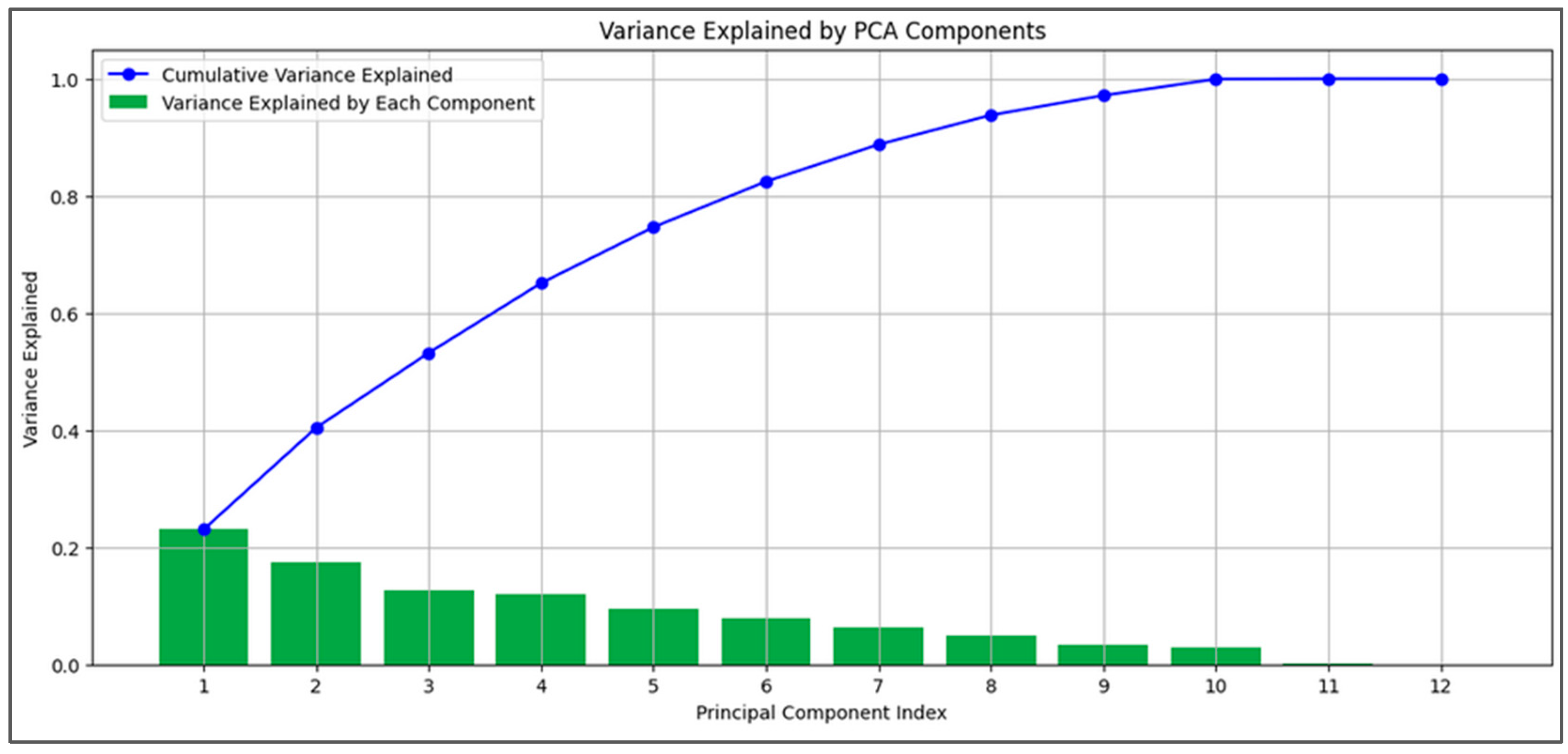
2.5. Principal Component Analysis (PCA)
2.6. Model Development
2.6.1. Model Selection and Rationale
2.6.2. Gradient Boosting Models (GBMs) and Random Forest (RF)
2.6.3. Sequential Models
2.6.4. Experiments’ Setup
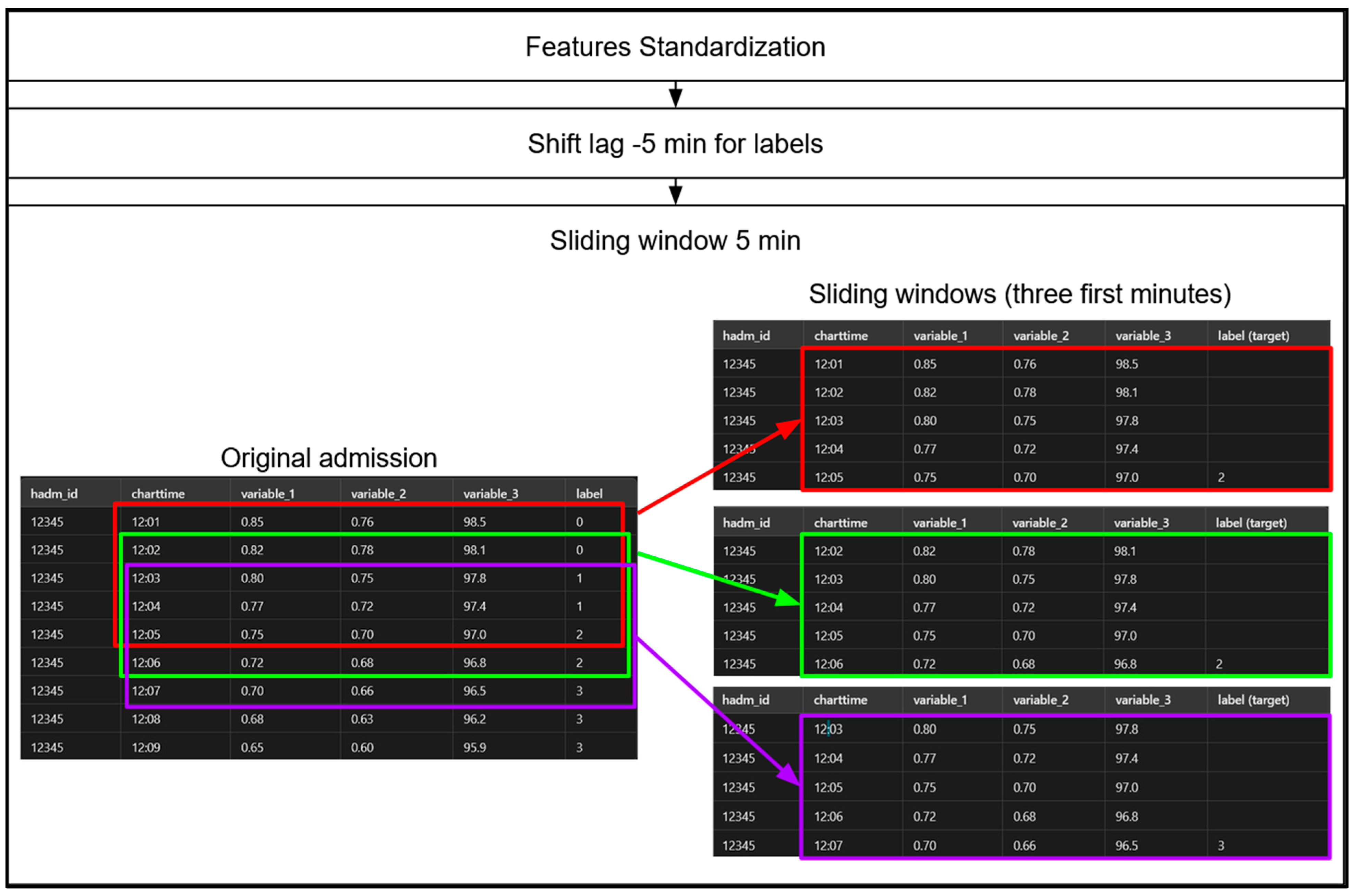
- Shift-Lag Method: Applied to predict hypoxemia severity scores 5 min in advance, providing a practical window for medical intervention (Figure 8). Indeed, in order to predict hypoxemia severity scores in advance, we apply a −5-min shift to the label values, aligning each row with the label observed 5 min later. This adjustment allows each row, containing physiological measurements recorded at a specific minute of a patient’s admission, to be used as input for predicting the hypoxemia severity score 5 min ahead. Importantly, this label-shifting technique is consistently implemented for both sequential models, Random Forest (RF) and gradient-boosting machines (GBMs).
- Class Imbalance Handling: Computed class weights inversely proportional to class frequencies.
- Hyperparameter Tuning of the GBMs and Random Forest (RF): We used the HyperOpt library, a popular tool for hyperparameter optimization, with two objective functions—AUC-based and log loss-based. HyperOpt employs the Tree-structured Parzen Estimator (TPE), a Bayesian optimization technique that iteratively updates a probabilistic model based on prior evaluations and performance metrics. Unlike traditional methods that treat these evaluations as independent, TPE refines its model progressively to capture the relationship between hyperparameters and performance, enhancing optimization efficiency.
- ○
- AUC-Based: This function focuses on maximizing the AUC score by minimizing 1 − AUC, which is especially beneficial when dealing with class imbalance.
- ○
- Log Loss: This function minimizes log loss (cross-entropy loss), assessing how closely the predicted probabilities match the actual labels, and penalizing incorrect or overly confident predictions.
3. Results
3.1. Dataset Characteristics
3.2. Imputation and Interpolation Outcomes
3.3. Exploratory Data Analysis Findings
3.4. Model Performance
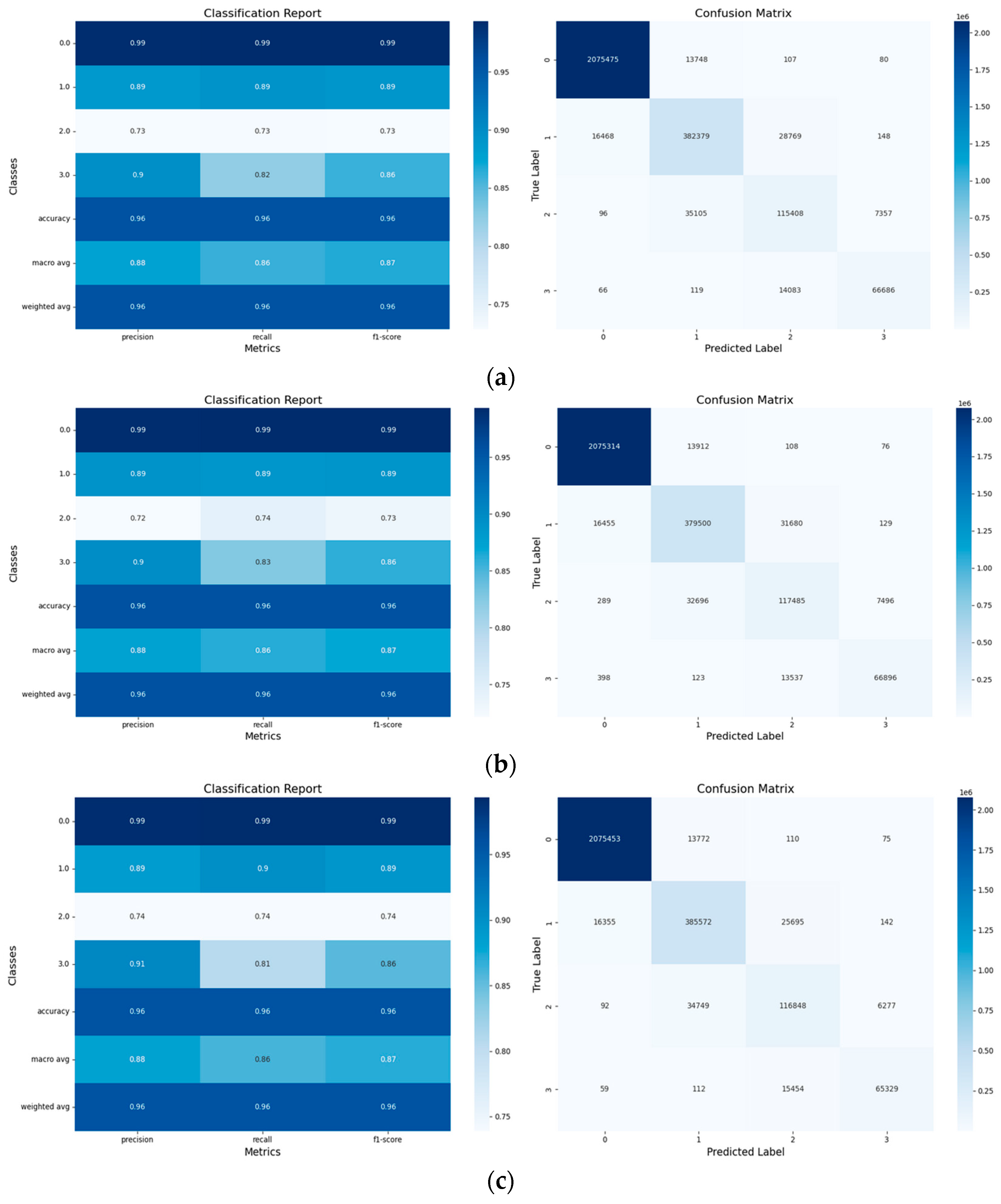
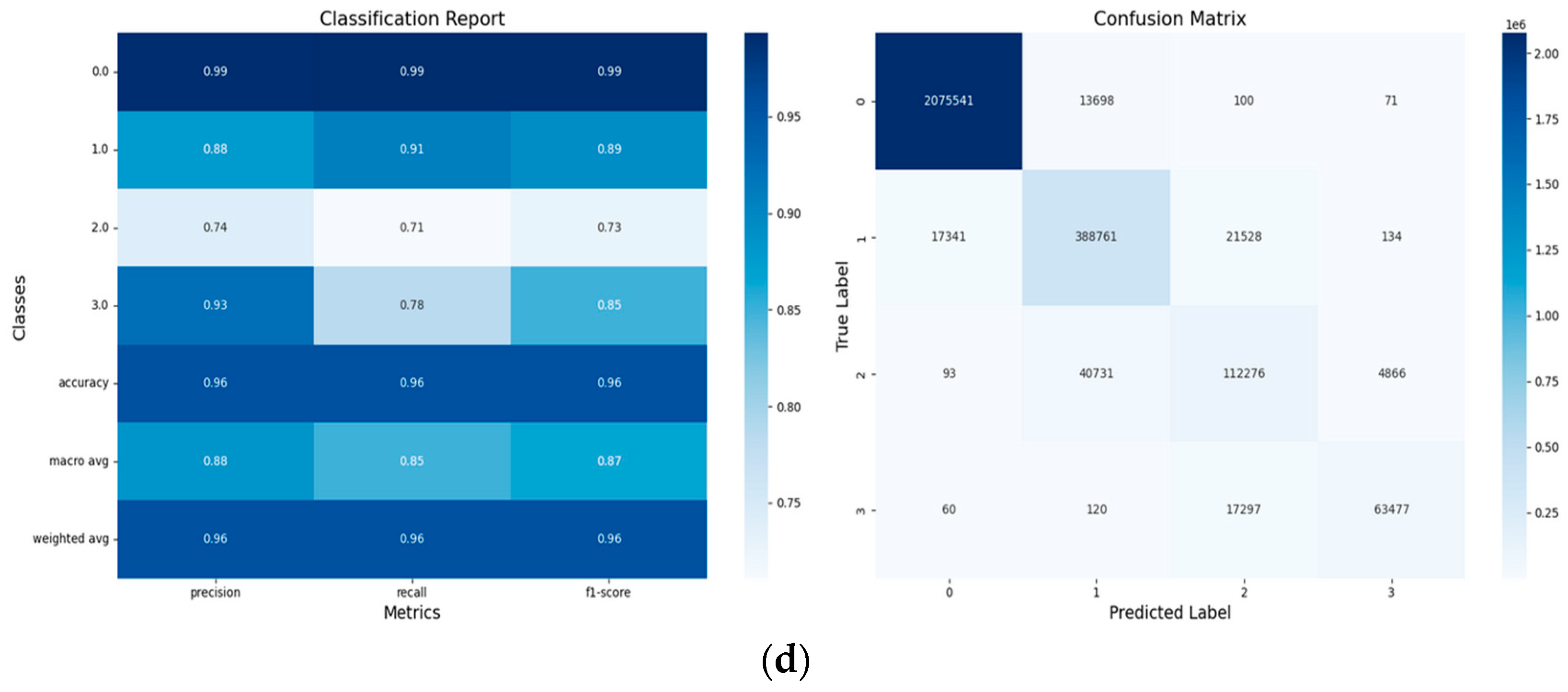
3.4.1. Tree-Based Models’ Results and Discussion
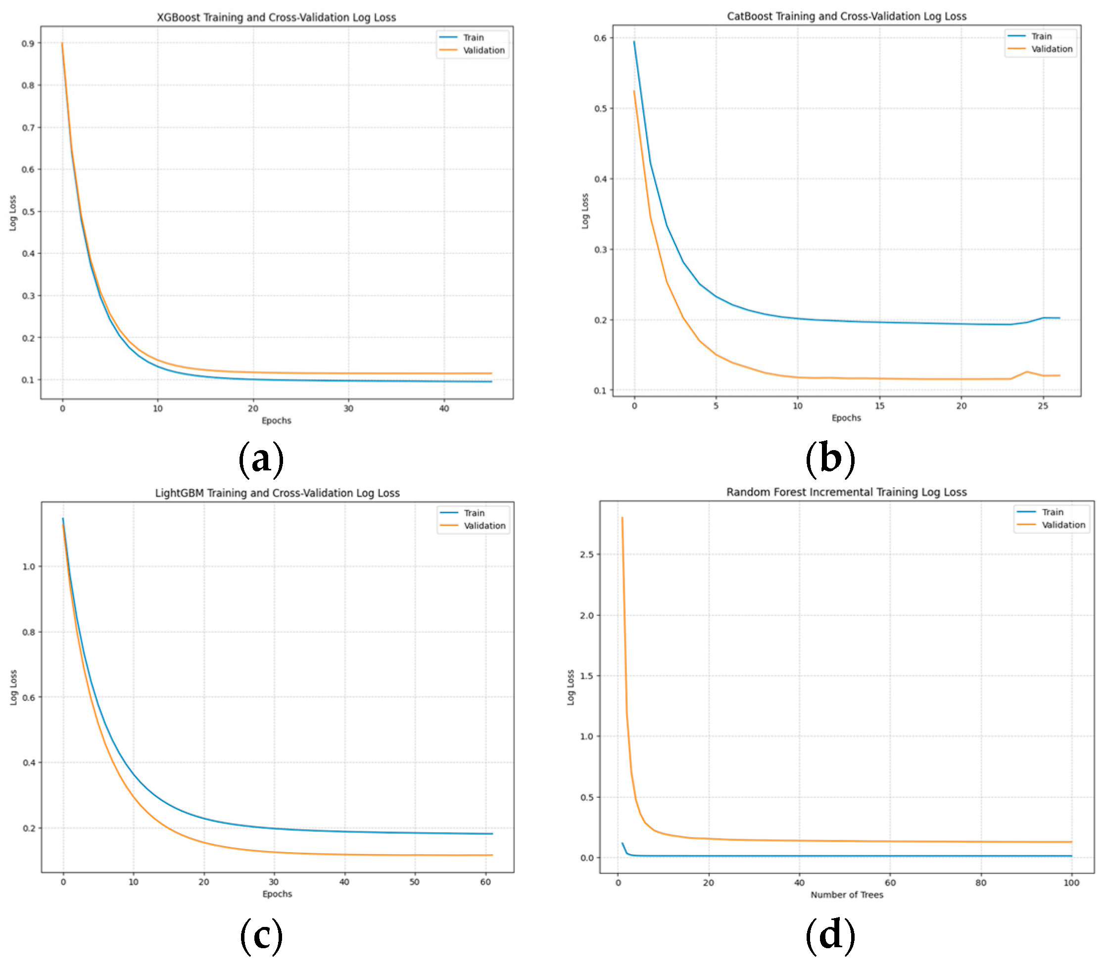
- Training and Convergence:
- Best Hyperparameters:
- Features Ablation Study:
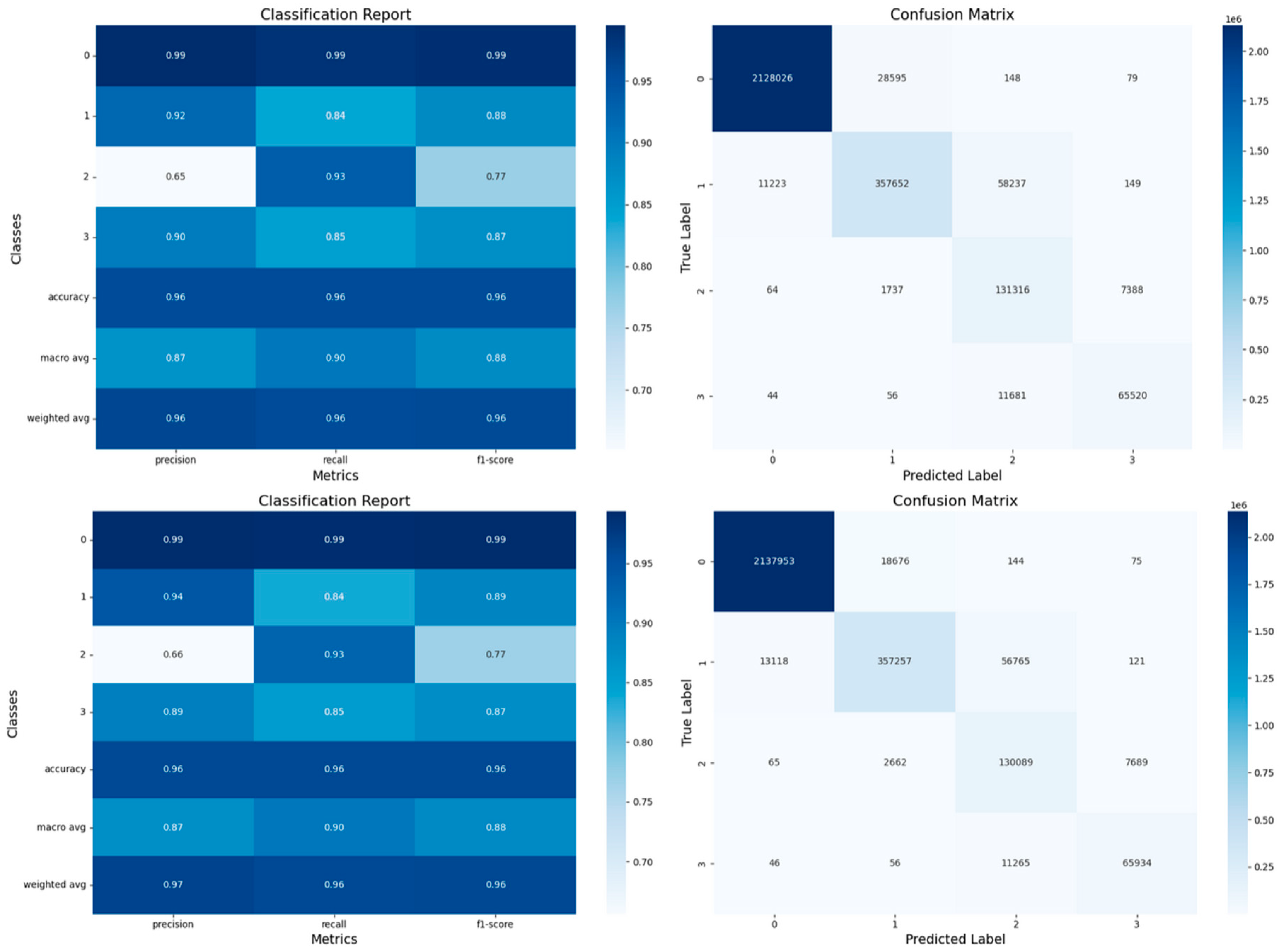
- Confusion Matrices:
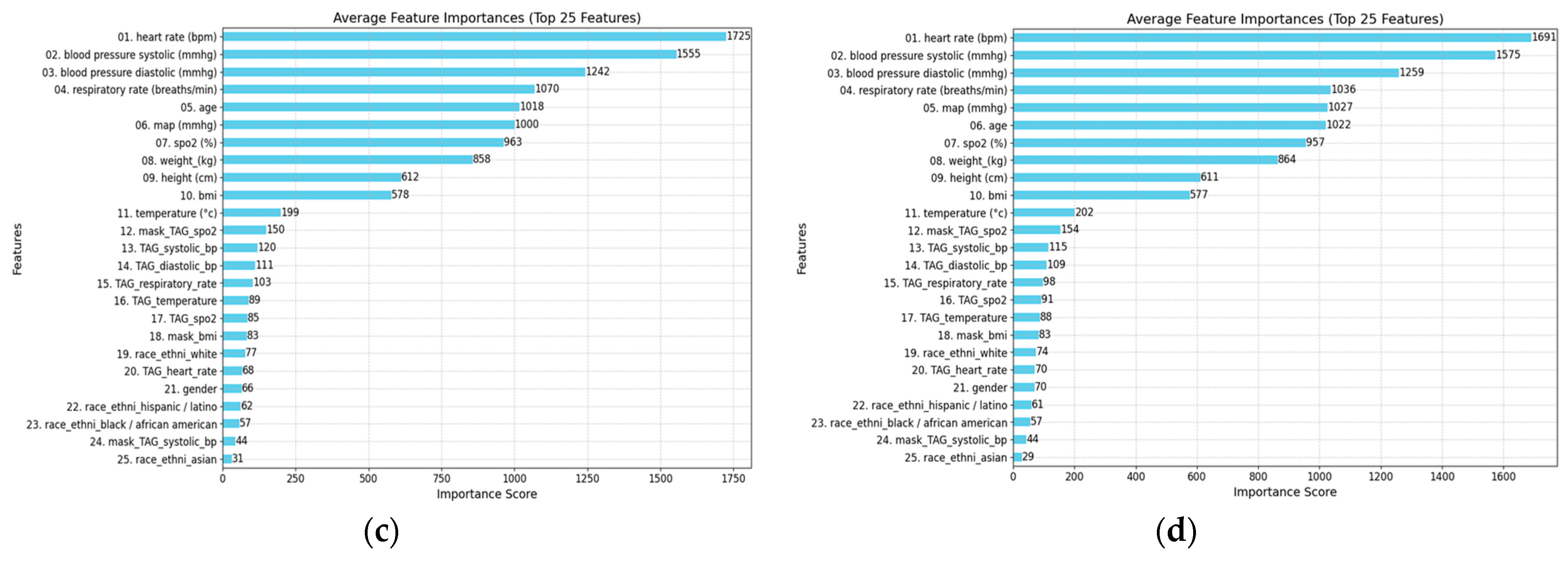
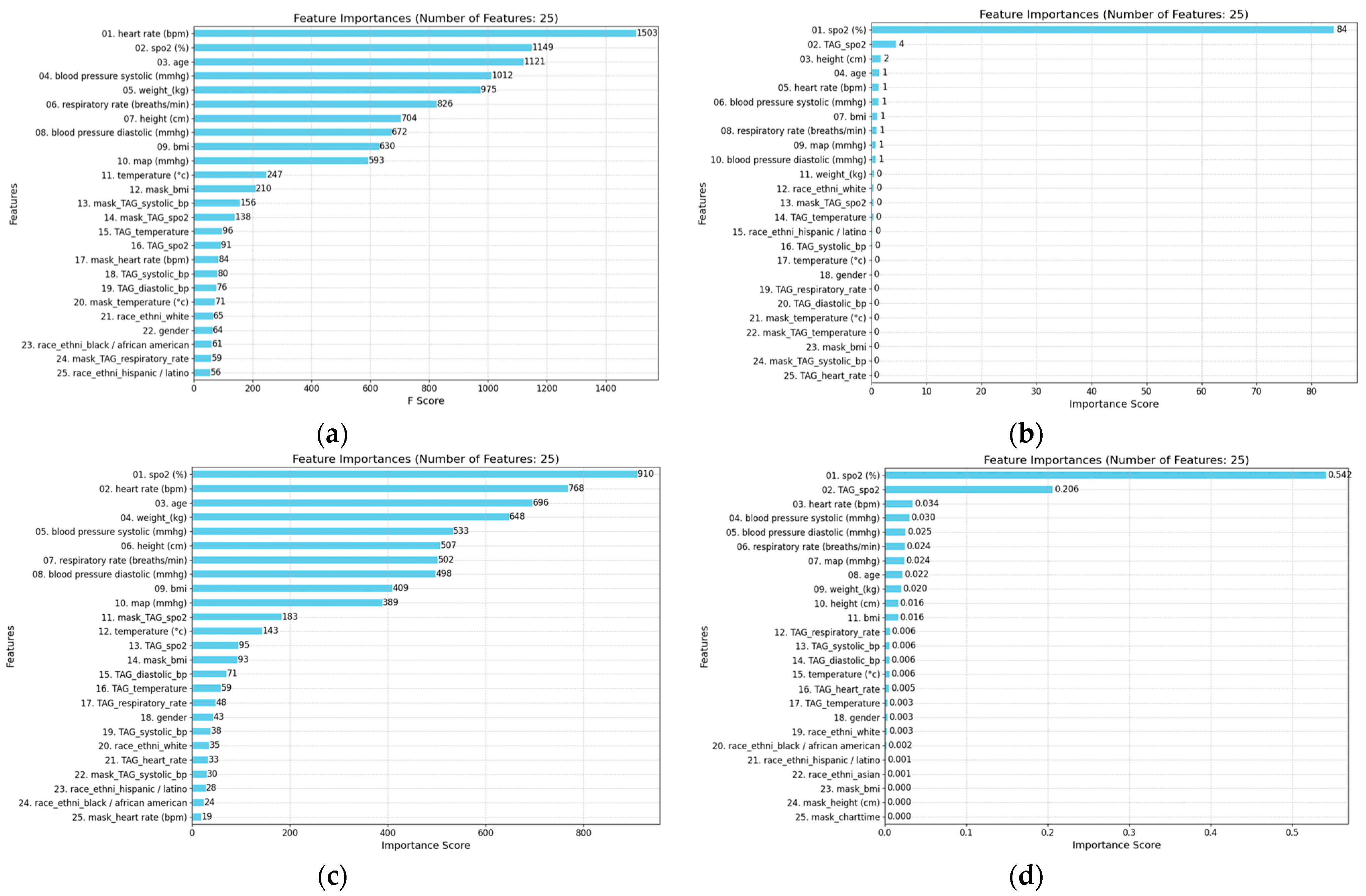
- Feature Importance and Model Interpretability:
- Performance Comparison of Ensemble Voting Classifiers with Tree-Based Models:
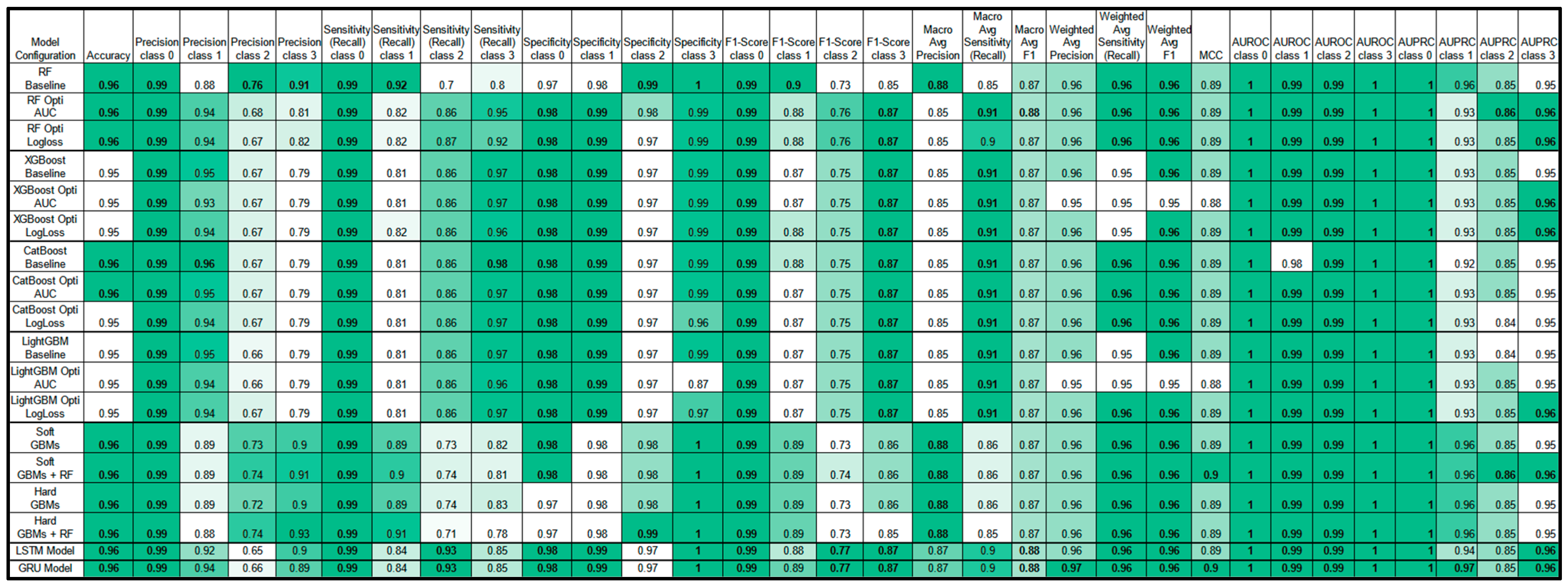
- Performance Metrics:
3.4.2. Sequential Models’ Results and Discussion
- Performance Metrics:
- Training Time:
3.4.3. Comparison Between GBMs, RF, and Sequential Models
- Performance Metrics:
4. Discussion
- Key Findings:
- Limitations and Perspectives:
- Implications for Practice:
- Future Work:
5. Conclusions
Author Contributions
Funding
Institutional Review Board Statement
Informed Consent Statement
Data Availability Statement
Acknowledgments
Conflicts of Interest
List of Acronyms
| SpO2 | peripheral oxygen saturation. |
| LSTM | long short-term memory. |
| PPV | positive predictive value. |
| SaO2 | arterial oxygen saturation. |
| GBT | gradient boosted tree. |
| AUROC | area under the receiver operating characteristics. |
| Lin | linear regression. |
| LR | logistic regression. |
| ANN | artificial neural network. |
| XGB | extreme gradient boosting. |
| RNN | recurrent neural network. |
| GBM | gradient boosting model. |
| PaO2 | partial pressure of oxygen. |
| FiO2 | fraction of oxygen in inhaled gas. |
| NN | neural network. |
| RF | random forest. |
| HR | heart rate. |
| BR | breath rate. |
| SBP | systolic blood pressure. |
| DBP | diastolic blood pressure. |
| AG | anion gap. |
| CNN | convolutional neural network. |
| MAE | mean averaged error to the range of values. |
| RF | random forest. |
| TBM | tree-based models. |
Appendix A


References
- Baker, D.J. Critical Care Requirements after Mass Toxic Agent Release. Crit. Care Med. 2005, 33, S66–S74. [Google Scholar] [CrossRef] [PubMed]
- Carli, P.; Telion, C.; Baker, D. Terrorism in France. Prehospital Disaster Med. 2003, 18, 92–99. [Google Scholar] [CrossRef] [PubMed]
- Okumura, T.; Suzuki, K.; Fukuda, A.; Kohama, A.; Takasu, N.; Ishimatsu, S.; Hinohara, S. The Tokyo Subway Sarin Attack: Disaster Management, Part 1: Community Emergency Response. Acad. Emerg. Med. 1998, 5, 613–617. [Google Scholar] [CrossRef] [PubMed]
- Bourassa, S.; Paquette-Raynard, E.; Noebert, D.; Dauphin, M.; Akinola, P.S.; Marseilles, J.; Jouvet, P.; Leclerc, J. Gaps in Prehospital Care for Patients Exposed to a Chemical Attack—A Systematic Review. Prehospital Disaster Med. 2022, 37, 230–239. [Google Scholar] [CrossRef] [PubMed]
- 39e Congrès de La Recherche Au CHU Sainte-Justine: 5–6 Février 2025. Available online: https://recherche.chusj.org/fr/congres2021 (accessed on 19 July 2024).
- Réseau de Recherche en Santé Respiratoire du Québec. Available online: https://rsr-qc.ca/jqrsr-2021/ (accessed on 28 November 2024).
- Inc, M.I.C. Medint Cbrne Group-Groupe Medint Cbrne. Available online: https://medintcbrne.com/projects-%26-projets (accessed on 19 July 2024).
- Bourassa, S. The Medical Management of Casualties in a Chemical Contaminated Environment: A Start for the CBRNE Defence Research Program for Clinicians. Ph.D. Thesis, Université de Montréal, Montréal, QC, Canada, 2023. [Google Scholar]
- Greenhalgh, T.; Treadwell, J.; Ms, R.B.; Roberts, N.; Tavare, A.; Pullyblank, A. Should We Use the NEWS (or NEWS2) Score When Assessing Patients with Possible COVID-19 in Primary Care? Additional Contributors (Topic Experts). 2020. Available online: https://www.researchgate.net/publication/340934244_Should_we_use_the_NEWS_or_NEWS2_score_when_assessing_patients_with_possible_COVID-19_in_primary_care?channel=doi&linkId=5ea5b751a6fdccd7945721c9&showFulltext=true (accessed on 28 November 2024).
- Alam, N.; Vegting, I.L.; Houben, E.; van Berkel, B.; Vaughan, L.; Kramer, M.H.H.; Nanayakkara, P.W.B. Exploring the Performance of the National Early Warning Score (NEWS) in a European Emergency Department. Resuscitation 2015, 90, 111–115. [Google Scholar] [CrossRef]
- Tavaré, A.; Pullyblank, A.; Redfern, E.; Collen, A.; Barker, R.O.; Gibson, A. NEWS2 in Out-of-Hospital Settings, the Ambulance and the Emergency Department. Clin. Med. 2022, 22, 525–529. [Google Scholar] [CrossRef]
- National Early Warning Score (NEWS) 2. Available online: https://www.rcp.ac.uk/improving-care/resources/national-early-warning-score-news-2/ (accessed on 24 October 2024).
- Paediatric Early Warning Score (PEWS). Available online: https://ihub.scot/improvement-programmes/scottish-patient-safety-programme-spsp/maternity-and-children-quality-improvement-collaborative-mcqic/paediatric-care/paediatric-early-warning-score-pews/ (accessed on 12 October 2023).
- Paediatric Observation Reference Ranges for Referrers. Available online: https://www.clinicalguidelines.scot.nhs.uk/rhc-for-health-professionals/referring-a-patient/paediatric-observation-reference-ranges-for-referrers/ (accessed on 3 July 2024).
- Akre, M.; Finkelstein, M.; Erickson, M.; Liu, M.; Vanderbilt, L.; Billman, G. Sensitivity of the Pediatric Early Warning Score to Identify Patient Deterioration. Pediatrics 2010, 125, e763–e769. [Google Scholar] [CrossRef]
- Chapman, S.M.; Maconochie, I.K. Early Warning Scores in Paediatrics: An Overview. Arch. Dis. Child. 2019, 104, 395–399. [Google Scholar] [CrossRef]
- Pediatric Vital Signs Normal Ranges|Iowa Head and Neck Protocols. Available online: https://medicine.uiowa.edu/iowaprotocols/pediatric-vital-signs-normal-ranges (accessed on 3 July 2024).
- Flynn, J.T.; Kaelber, D.C.; Baker-Smith, C.M.; Blowey, D.; Carroll, A.E.; Daniels, S.R.; de Ferranti, S.D.; Dionne, J.M.; Falkner, B.; Flinn, S.K.; et al. Clinical Practice Guideline for Screening and Management of High Blood Pressure in Children and Adolescents. Pediatrics 2017, 140, e20171904. [Google Scholar] [CrossRef]
- Validation of a Modified Early Warning Score in Medical Admissions. Available online: https://read.qxmd.com/read/11588210/validation-of-a-modified-early-warning-score-in-medical-admissions (accessed on 3 July 2024).
- Khan, A.; Sarma, D.; Gowda, C.; Rodrigues, G. The Role of Modified Early Warning Score (MEWS) in the Prognosis of Acute Pancreatitis. Oman Med. J. 2021, 36, e272. [Google Scholar] [CrossRef]
- Effect of Introducing the Modified Early Warning Score on Clinical Outcomes, Cardio-Pulmonary Arrests and Intensive Care Utilisation in Acute Medical Admissions. Available online: https://read.qxmd.com/read/12859475/effect-of-introducing-the-modified-early-warning-score-on-clinical-outcomes-cardio-pulmonary-arrests-and-intensive-care-utilisation-in-acute-medical-admissions (accessed on 3 July 2024).
- Smith, M.E.B.; Chiovaro, J.C.; O’Neil, M.; Kansagara, D.; Quiñones, A.R.; Freeman, M.; Motu’apuaka, M.L.; Slatore, C.G. Early Warning System Scores for Clinical Deterioration in Hospitalized Patients: A Systematic Review. Ann. Am. Thorac. Soc. 2014, 11, 1454–1465. [Google Scholar] [CrossRef] [PubMed]
- Gerry, S.; Bonnici, T.; Birks, J.; Kirtley, S.; Virdee, P.S.; Watkinson, P.J.; Collins, G.S. Early Warning Scores for Detecting Deterioration in Adult Hospital Patients: Systematic Review and Critical Appraisal of Methodology. BMJ 2020, 369, m1501. [Google Scholar] [CrossRef] [PubMed]
- Downey, C.L.; Tahir, W.; Randell, R.; Brown, J.M.; Jayne, D.G. Strengths and Limitations of Early Warning Scores: A Systematic Review and Narrative Synthesis. Int. J. Nurs. Stud. 2017, 76, 106–119. [Google Scholar] [CrossRef] [PubMed]
- Fu, L.-H.; Schwartz, J.; Moy, A.; Knaplund, C.; Kang, M.-J.; Schnock, K.O.; Garcia, J.P.; Jia, H.; Dykes, P.C.; Cato, K.; et al. Development and Validation of Early Warning Score System: A Systematic Literature Review. J. Biomed. Inform. 2020, 105, 103410. [Google Scholar] [CrossRef]
- Shamout, F.E.; Zhu, T.; Sharma, P.; Watkinson, P.J.; Clifton, D.A. Deep Interpretable Early Warning System for the Detection of Clinical Deterioration. IEEE J. Biomed. Health Inform. 2020, 24, 437–446. [Google Scholar] [CrossRef]
- Lauritsen, S.M.; Kristensen, M.; Olsen, M.V.; Larsen, M.S.; Lauritsen, K.M.; Jørgensen, M.J.; Lange, J.; Thiesson, B. Explainable Artificial Intelligence Model to Predict Acute Critical Illness from Electronic Health Records. Nat. Commun. 2020, 11, 3852. [Google Scholar] [CrossRef]
- Pigat, L.; Geisler, B.P.; Sheikhalishahi, S.; Sander, J.; Kaspar, M.; Schmutz, M.; Rohr, S.O.; Wild, C.M.; Goss, S.; Zaghdoudi, S.; et al. Predicting Hypoxia Using Machine Learning: Systematic Review. JMIR Med. Inform. 2024, 12, e50642. [Google Scholar] [CrossRef]
- Johnson, A.; Pollard, T.; Mark, R. MIMIC-III Clinical Database 2015. Available online: https://physionet.org/content/mimiciii/1.4/ (accessed on 28 November 2024).
- Johnson, A.E.W.; Pollard, T.J.; Shen, L.; Lehman, L.H.; Feng, M.; Ghassemi, M.; Moody, B.; Szolovits, P.; Anthony Celi, L.; Mark, R.G. MIMIC-III, a Freely Accessible Critical Care Database. Sci. Data 2016, 3, 160035. [Google Scholar] [CrossRef]
- Johnson, A.E.W.; Bulgarelli, L.; Shen, L.; Gayles, A.; Shammout, A.; Horng, S.; Pollard, T.J.; Hao, S.; Moody, B.; Gow, B.; et al. MIMIC-IV, a Freely Accessible Electronic Health Record Dataset. Sci. Data 2023, 10, 1. [Google Scholar] [CrossRef]
- Ke, G.; Meng, Q.; Finley, T.; Wang, T.; Chen, W.; Ma, W.; Ye, Q.; Liu, T.-Y. LightGBM: A Highly Efficient Gradient Boosting Decision Tree. In Proceedings of the Advances in Neural Information Processing Systems, Long Beach, CA, USA, 4–9 December 2017; Curran Associates, Inc.: Red Hook, NY, USA, 2017; Volume 30. [Google Scholar]
- Prokhorenkova, L.; Gusev, G.; Vorobev, A.; Dorogush, A.V.; Gulin, A. CatBoost: Unbiased Boosting with Categorical Features. Adv. Neural Inf. Process. Syst. 2018, 31. [Google Scholar]
- Chen, T.; Guestrin, C. XGBoost: A Scalable Tree Boosting System. In Proceedings of the 22nd ACM SIGKDD International Conference on Knowledge Discovery and Data Mining, San Francisco, CA, USA, 13–17 August 2016; ACM: San Francisco, CA, USA, 2016; pp. 785–794. [Google Scholar]
- Gers, F.A.; Schmidhuber, J.; Cummins, F. Learning to Forget: Continual Prediction with LSTM. In Proceedings of the 1999 Ninth International Conference on Artificial Neural Networks ICANN 99, (Conf. Publ. No. 470), Edinburgh, UK, 7–10 September 1999; Volume 2, pp. 850–855. [Google Scholar]
- Chung, J.; Gulcehre, C.; Cho, K.; Bengio, Y. Empirical Evaluation of Gated Recurrent Neural Networks on Sequence Modeling. Available online: https://arxiv.org/abs/1412.3555v1 (accessed on 20 July 2024).
- Hochreiter, S.; Schmidhuber, J. Long Short-Term Memory. Neural Comput. 1997, 9, 1735–1780. [Google Scholar] [CrossRef] [PubMed]
- Dempsey, J.A.; Wagner, P.D. Exercise-Induced Arterial Hypoxemia. J. Appl. Physiol. 1999, 87, 1997–2006. [Google Scholar] [CrossRef] [PubMed]
- Johannigman, J.; Gerlach, T.; Cox, D.; Juhasz, J.; Britton, T.; Elterman, J.; Rodriquez, D.; Blakeman, T.; Branson, R. Hypoxemia during Aeromedical Evacuation of the Walking Wounded. J. Trauma Acute Care Surg. 2015, 79, S216–S220. [Google Scholar] [CrossRef] [PubMed]
- Bourassa, S.; Bouchard, P.-A.; Dauphin, M.; Lellouche, F. Oxygen Conservation Methods with Automated Titration. Respir. Care 2020, 65, 1433–1442. [Google Scholar] [CrossRef]
- Samad, M.D.; Abrar, S.; Diawara, N. Missing Value Estimation Using Clustering and Deep Learning within Multiple Imputation Framework. Knowl.-Based Syst. 2022, 249, 108968. [Google Scholar] [CrossRef]
- Perez-Lebel, A.; Varoquaux, G.; Le Morvan, M.; Josse, J.; Poline, J.-B. Benchmarking Missing-Values Approaches for Predictive Models on Health Databases. GigaScience 2022, 11, giac013. [Google Scholar] [CrossRef]
- Josse, J.; Chen, J.M.; Prost, N.; Scornet, E.; Varoquaux, G. On the Consistency of Supervised Learning with Missing Values. Stat. Pap. 2024, 65, 5447–5479. [Google Scholar] [CrossRef]
- Sharafoddini, A.; Dubin, J.A.; Maslove, D.M.; Lee, J. A New Insight Into Missing Data in Intensive Care Unit Patient Profiles: Observational Study. JMIR Med. Inform. 2019, 7, e11605. [Google Scholar] [CrossRef]
- Sperrin, M.; Martin, G.P.; Sisk, R.; Peek, N. Missing Data Should Be Handled Differently for Prediction than for Description or Causal Explanation. J. Clin. Epidemiol. 2020, 125, 183–187. [Google Scholar] [CrossRef]
- Kusters, R.; Misevic, D.; Berry, H.; Cully, A.; Le Cunff, Y.; Dandoy, L.; Díaz-Rodríguez, N.; Ficher, M.; Grizou, J.; Othmani, A.; et al. Interdisciplinary Research in Artificial Intelligence: Challenges and Opportunities. Front. Big Data 2020, 3. [Google Scholar] [CrossRef]
- Lundberg, S.M.; Nair, B.; Vavilala, M.S.; Horibe, M.; Eisses, M.J.; Adams, T.; Liston, D.E.; Low, D.K.-W.; Newman, S.-F.; Kim, J.; et al. Explainable Machine-Learning Predictions for the Prevention of Hypoxaemia during Surgery. Nat. Biomed. Eng. 2018, 2, 749. [Google Scholar] [CrossRef] [PubMed]
- Annapragada, A.V.; Greenstein, J.L.; Bose, S.N.; Winters, B.D.; Sarma, S.V.; Winslow, R.L. SWIFT: A Deep Learning Approach to Prediction of Hypoxemic Events in Critically-Ill Patients Using SpO2 Waveform Prediction. PLOS Comput. Biol. 2021, 17, e1009712. [Google Scholar] [CrossRef] [PubMed]
- Bureau, U.C. About the Topic of Race. Available online: https://www.census.gov/topics/population/race/about.html (accessed on 15 July 2024).
- Lassman, D.; Hartman, M.; Washington, B.; Andrews, K.; Catlin, A. US Health Spending Trends By Age And Gender: Selected Years 2002–2010. Health Aff. 2014, 33, 815–822. [Google Scholar] [CrossRef] [PubMed]
- González-Nóvoa, J.A.; Busto, L.; Rodríguez-Andina, J.J.; Fariña, J.; Segura, M.; Gómez, V.; Vila, D.; Veiga, C. Using Explainable Machine Learning to Improve Intensive Care Unit Alarm Systems. Sensors 2021, 21, 7125. [Google Scholar] [CrossRef]
- Breiman, L. Random Forests. Mach. Learn. 2001, 45, 5–32. [Google Scholar] [CrossRef]
- Hyland, S.L.; Faltys, M.; Hüser, M.; Lyu, X.; Gumbsch, T.; Esteban, C.; Bock, C.; Horn, M.; Moor, M.; Rieck, B. Early Prediction of Circulatory Failure in the Intensive Care Unit Using Machine Learning. Nat. Med. 2020, 26, 364–373. [Google Scholar] [CrossRef]
- Zheng, J.; Li, J.; Zhang, Z.; Yu, Y.; Tan, J.; Liu, Y.; Gong, J.; Wang, T.; Wu, X.; Guo, Z. Clinical Data Based XGBoost Algorithm for Infection Risk Prediction of Patients with Decompensated Cirrhosis: A 10-Year (2012–2021) Multicenter Retrospective Case-Control Study. BMC Gastroenterol. 2023, 23, 310. [Google Scholar] [CrossRef]
- Zhao, H.; Ma, Z.; Sun, Y. Predict Onset Age of Hypertension Using CatBoost and Medical Big Data. In Proceedings of the 2020 International Conference on Networking and Network Applications (NaNA), Haikou, China, 11–14 December 2020; pp. 405–409. [Google Scholar]
- Pham, T.D. Time–Frequency Time–Space LSTM for Robust Classification of Physiological Signals. Sci. Rep. 2021, 11, 6936. [Google Scholar] [CrossRef]
- Lipton, Z.C.; Kale, D.C.; Elkan, C.; Wetzel, R. Learning to Diagnose with LSTM Recurrent Neural Networks. arXiv 2015, arXiv:1511.03677. [Google Scholar]
- Mishra, S.; Tiwari, N.K.; Kumari, K.; Kumawat, V. Prediction of Heart Disease Using Machine Learning. In Proceedings of the 2023 2nd International Conference on Applied Artificial Intelligence and Computing (ICAAIC), Salem, India, 4–6 May 2023; pp. 1617–1621. [Google Scholar]
- Moreno-Sanchez, P.A. Development of an Explainable Prediction Model of Heart Failure Survival by Using Ensemble Trees. In Proceedings of the 2020 IEEE International Conference on Big Data (Big Data), Virtual Event, 10–13 December 2020; pp. 4902–4910. [Google Scholar]
- Temel, G.; Ankarali, H.; Taşdelen, B.; Erdoğan, S.; Özge, A. A Comparison of Boosting Tree and Gradient Treeboost Methods for Carpal Tunnel Syndrome. Turk. Klin. J. Biostat. 2014, 6, 67. [Google Scholar]
- Yang, Y. Prediction of Blood Oxygen Saturation Based on Deep Learning. In Proceedings of the International Conference on Algorithms, Microchips and Network Applications, Zhuhai, China, 6 May 2022; Volume 12176, p. 1217602. [Google Scholar]
- Ma, F.; Chitta, R.; Zhou, J.; You, Q.; Sun, T.; Gao, J. Dipole: Diagnosis Prediction in Healthcare via Attention-Based Bidirectional Recurrent Neural Networks. In Proceedings of the 23rd ACM SIGKDD International Conference on Knowledge Discovery and Data Mining, Halifax, NS, Canada, 13 August 2017; pp. 1903–1911. [Google Scholar]
- Parkinson’s Disease Detection Using Hybrid LSTM-GRU Deep Learning Model. Available online: https://www.mdpi.com/2079-9292/12/13/2856 (accessed on 28 November 2024).
- Suo, Q.; Ma, F.; Canino, G.; Gao, J.; Zhang, A.; Veltri, P.; Agostino, G. A Multi-Task Framework for Monitoring Health Conditions via Attention-Based Recurrent Neural Networks. AMIA. Annu. Symp. Proc. 2018, 2017, 1665–1674. [Google Scholar] [PubMed]
- Shwartz-Ziv, R.; Armon, A. Tabular Data: Deep Learning Is Not All You Need. Inf. Fusion 2022, 81, 84–90. [Google Scholar] [CrossRef]
- Weitz, J.I.; Fredenburgh, J.C.; Eikelboom, J.W. A Test in Context: D-Dimer. J. Am. Coll. Cardiol. 2017, 70, 2411–2420. [Google Scholar] [CrossRef] [PubMed]
- Bouillon-Minois, J.-B.; Roux, V.; Jabaudon, M.; Flannery, M.; Duchenne, J.; Dumesnil, M.; Paillard-Turenne, M.; Gendre, P.-H.; Grapin, K.; Rieu, B.; et al. Impact of Air Transport on SpO2/FiO2 among Critical COVID-19 Patients during the First Pandemic Wave in France. J. Clin. Med. 2021, 10, 5223. [Google Scholar] [CrossRef]
- Chen, W.; Janz, D.R.; Shaver, C.M.; Bernard, G.R.; Bastarache, J.A.; Ware, L.B. Clinical Characteristics and Outcomes Are Similar in ARDS Diagnosed by Oxygen Saturation/Fio2 Ratio Compared with Pao2/Fio2 Ratio. Chest 2015, 148, 1477–1483. [Google Scholar] [CrossRef]
- Faltys, M.; Zimmermann, M.; Lyu, X.; Hüser, M.; Hyland, S.; Rätsch, G.; Merz, T. HiRID, a High Time-Resolution ICU Dataset. Available online: https://physionet.org/content/hirid/1.1.1/ (accessed on 28 November 2024).


| Population | Severe | Moderate | Mild | Normal |
|---|---|---|---|---|
| Adults without COPD | ≤91% | 92–93% | 94–95% | 96–100% |
| Adults with COPD | ≤82% | 83–84% | 85–87% | 88–92% |
| Pediatric (without COPD) | ≤84% | 85–88% | 89–95% | 96–100% |
| Age Group | Severe Low (Level 3) | Moderate Low (Level 2) | Mild Low (Level 1) | Normal Beseline (Level 0) | Mild High (Level 1) | Moderate High (Level 2) | Severe High (Level 3) |
|---|---|---|---|---|---|---|---|
| Adults | |||||||
| Respiratory Rate (BPM) | 0–5 | 6–7 | 8–9 | 10–20 | 21–25 | 26–29 | 30–400 |
| Saturation (SpO2, %) | 0–84 | 85–88 | 89–95 | 96–100 | N/A: Ambient Air | N/A: Ambient Air | N/A: Ambient Air |
| Heart Rate (BPM) | 0–40 | 41–50 | 51–59 | 60–90 | 91–110 | 111–130 | 131–400 |
| Systolic BP (mmHg) | 0–90 | 91–100 | 101–114 | 115–119 | 120–129 | 130–144 | 145–300 |
| Diastolic BP (mmHg) | 0–49 | 50–59 | 60–64 | 65–79 | 80–85 | 86–90 | 91–300 |
| Temperature (°C) | 0–35.0 | 35.1–35.9 | 36.0–36.6 | 36.7–37.7 | 37.8–38.8 | 38.9–39.8 | 39.9–60 |
| 0–11 Months | |||||||
| Respiratory Rate (BPM) | ≤19 | 20–24 | 25–29 | 30–49 | 50–59 | 60–69 | ≥70 |
| Saturation (SpO2, %) | ≤91 | 92 | 93 | 94–100 | N/A: Ambient Air | N/A: Ambient Air | N/A: Ambient Air |
| Heart Rate (BPM) | ≤99 | 100–104 | 105–109 | 110–159 | 160–164 | 165–169 | ≥170 |
| Systolic BP (mmHg) | ≤59 | 60–64 | 65–69 | 70–99 | 100–104 | 105–109 | ≥110 |
| Diastolic BP (mmHg) | ≤20 | 19–26 | 27–37 | 37–56 | 57–69 | 70–89 | ≥90 |
| Temperature (°C) | ≤34.9 | 35.3–35.4 | 35.5–35.9 | 36–37.0 | 37.1–37.4 | 37.5–37.9 | ≥38 |
| 12–23 Months | |||||||
| Respiratory Rate (BPM) | ≤19 | 20–22 | 23–24 | 25–39 | 40–49 | 50–59 | ≥60 |
| Saturation (SpO2, %) | ≤91 | 92 | 93 | 94–100 | N/A: Ambient Air | N/A: Ambient Air | N/A: Ambient Air |
| Heart Rate (BPM) | ≤79 | 80–89 | 90–99 | 100–149 | 150–154 | 155–159 | ≥160 |
| Systolic BP (mmHg) | ≤59 | 60–64 | 65–69 | 70–99 | 100–104 | 105–109 | ≥110 |
| Diastolic BP (mmHg) | ≤20 | 19–35 | 36–40 | 41–62 | 63–70 | 71–89 | ≥90 |
| Temperature (°C) | ≤34.9 | 35.3–35.4 | 35.5–35.9 | 36–37.0 | 37.1–37.4 | 37.5–37.9 | ≥38 |
| 2–4 Years | |||||||
| Respiratory Rate (BPM) | ≤14 | 15–18 | 17–19 | 20–34 | 35–39 | 40–49 | ≥50 |
| Saturation (SpO2, %) | ≤91 | 92 | 93 | ≥94 | N/A: Ambient Air | N/A: Ambient Air | N/A: Ambient Air |
| Heart Rate (BPM) | ≤69 | 70–79 | 80–89 | 90–139 | 140–144 | 145–149 | ≥150 |
| Systolic BP (mmHg) | ≤69 | 70–79 | N/A | 80–99 | N/A | 100–119 | ≥120 |
| Diastolic BP (mmHg) | ≤18 | 19–34 | 35–43 | 44–67 | 68–75 | 76–89 | ≥90 |
| Temperature (°C) | ≤34.9 | 35.3–35.4 | 35.5–35.9 | 36–37.0 | 37.1–37.4 | 37.5–37.9 | ≥38 |
| 5–11 Years | |||||||
| Respiratory Rate (BPM) | ≤14 | 15–16 | 17–19 | 20–29 | 30–34 | 35–39 | ≥40 |
| Saturation (SpO2, %) | ≤91 | 92 | 93 | ≥94 | N/A: Ambient Air | N/A: Ambient Air | N/A: Ambient Air |
| Heart Rate (BPM) | ≤59 | 60–69 | 70–79 | 80–129 | 130–134 | 135–139 | ≥140 |
| Systolic BP (mmHg) | ≤79 | 80–84 | 85–89 | 90–109 | 110–119 | 120–129 | ≥130 |
| Diastolic BP (mmHg) | ≤41 | 42–47 | 48–52 | 53–79 | 80–85 | 86–89 | ≥90 |
| Temperature (°C) | ≤34.9 | 35.3–35.4 | 35.5–35.9 | 36–37.0 | 37.1–37.4 | 37.5–37.9 | ≥38 |
| 12–17 Years | |||||||
| Respiratory Rate (BPM) | ≤9 | 10–12 | 13–14 | 15–24 | 25–29 | 30–34 | ≥35 |
| Saturation (SpO2, %) | ≤91 | 92 | 93 | ≥94 | N/A: Ambient Air | N/A: Ambient Air | N/A: Ambient Air |
| Heart Rate (BPM) | ≤49 | 50–59 | 60–69 | 70–109 | 110–119 | 120–129 | ≥130 |
| Systolic BP (mmHg) | ≤89 | 90–94 | 95–99 | 100–119 | 120–134 | 135–139 | ≥140 |
| Diastolic BP (mmHg) | ≤41 | 42–47 | 48–52 | 63–80 | 81–85 | 86–89 | ≥90 |
| Temperature (°C) | ≤34.9 | 35.3–35.4 | 35.5–35.9 | 36–37.0 | 37.1–37.4 | 37.5–37.9 | ≥38 |
| Polynomial (Order 3 and 5) and Cubic Spline Interpolations | Linear Interpolations | |||
|---|---|---|---|---|
| Variable | Minimal | Maximal | Minimal | Maximal |
| Respiratory rate (breaths/min) | −7.36 × 10¹⁰ | 2.51 × 10¹⁴ | 0 | 121 |
| Spo2 (%) | −3.78 × 10⁹ | 1.81 × 10¹⁴ | 0 | 100 |
| Heart rate (bpm) | −8.62 × 10¹³ | 2.52 × 10¹⁰ | 0 | 268 |
| Blood pressure systolic (mmhg) | −1.22 × 10¹¹ | 3.82 × 10¹⁰ | 0 | 261 |
| Blood pressure diastolic (mmhg) | −7.30 × 10¹⁰ | 5.74 × 10⁸ | 0 | 228 |
| MAP(mmhg) | −8.32 × 10¹⁰ | 1.07 × 10¹⁰ | 0 | 238 |
| Category | Subcategory (Years) | Count | Percentage (%) |
|---|---|---|---|
| Age Stratification | <1 year | 0 | 0 |
| 1 to <2 | 0 | 0 | |
| 2 to 4 | 0 | 0 | |
| 5 to 11 | 0 | 0 | |
| 12 to 17 | 4 | 0.061369 | |
| 18 to 45 | 836 | 12.826202 | |
| 46 to 65 | 2369 | 36.345505 | |
| 66 to 85 | 2693 | 41.316355 | |
| 86+ | 616 | 9.450752 | |
| Gender | Male | 3511 | 53.866217 |
| Female | 3007 | 46.133783 | |
| Race/Ethnicity | White | 4652 | 71.371586 |
| Undefined | 694 | 10.647438 | |
| Black/African American | 686 | 10.524701 | |
| Hispanic/Latino | 259 | 3.973612 | |
| Asian | 199 | 3.053084 | |
| American Indian/ Alaska Native | 13 | 0.199448 | |
| Native Hawaiian/ other Pacific Islander | 9 | 0.138079 | |
| Multiracial | 6 | 0.092053 |
| Feature Name | Description | Measurement Units |
|---|---|---|
| Gender | Biological gender of the patient. | N/A |
| Age | Age of the patient. | Years |
| Weight | Body weight of the patient. | Kilograms (kg) |
| Height | Body height of the patient. | Centimeters (cm) |
| BMI | Body Mass Index, widely used metric to assess body weight relative to height, providing a quick estimate of body fatness for most individuals. | N/A |
| Blood Pressure Systolic | Systolic blood pressure of the patient. | mmHg |
| Blood Pressure Diastolic | Diastolic blood pressure of the patient. | mmHg |
| MAP | Mean Arterial Pressure (MAP), an important cardiovascular metric representing the average pressure in a person’s arteries during one cardiac cycle. | mmHg |
| Temperature | Body temperature of the patient. | Degrees Celsius (°C) |
| Heart Rate | Number of heartbeats per minute. | Beats per minute (bpm) |
| Respiratory Rate | Number of breaths per minute. | Breaths per minute |
| Oxygen Saturation (SpO2) | Oxygen level in the blood. | Percentage (%) |
| Ethnicity or Race | Ethnicity or race of the patient, including Native Hawaiian/Other Pacific Islander, American Indian/Alaska Native, Black/African American, Asian, Multiracial, Hispanic/Latino (classified as an ethnicity), and White. | N/A |
| TAG_ | Derived feature scores based on NEWS2+ for six key physiological variables: TAG_Heart_Rate, TAG_Temperature, TAG_SpO2, TAG_Diastolic_BP, TAG_Systolic_BP, TAG_Respiratory_Rate. | N/A |
| Mask_ | Indicates if values are synthetic (i.e., interpolated or imputed, by 1) or original (by 0) for the following variables: SpO2, Systolic_BP, Diastolic_BP, Respiratory Rate, Temperature, BMI, Heart Rate, MAP, Height, Weight, and the six TAG_. | N/A |
| Label (output to be predicted, as a classification task) | Hypoxemia severity score based on the NEWS2+ scoring matrices for adults without COPD, adults with COPD, and pediatric populations (see part 2.3.1 for the labelization process) | centimeters (cm) |
| Before Interpolation | After Interpolation | |||
|---|---|---|---|---|
| Label (Hypoxemia Severity Score) | Count | Percentage (%) | Count | Percentage (%) |
| 0 | 729,657 | 72.2369 | 17,450,087 | 76.86217 |
| 1 | 158,419 | 15.68367 | 3,293,482 | 14.50676 |
| 2 | 73,338 | 7.260548 | 1,244,804 | 5.482972 |
| 3 | 48,675 | 4.818882 | 714,716 | 3.1481 |
| Model Classifier (Multi-Class) | Setup (Default Hyperparameters) | Tuned Hyperparameters (HyperOpt Library) |
|---|---|---|
| XGBoost | - Objective: ‘multi:softmax’ function - Number of Classes: 4 - Random Seed: 42 - Evaluation Metric: ‘mlogloss’ - Number of Boosting Rounds: 300 - Early Stopping Rounds: 5 - Device: GPU | - max_depth: 4 to 8 - eta: 0.005 to 0.3 - subsample: 0.5 to 1 - gamma: 0 to 22 - min_child_weight: 0 to 15 |
| CatBoost | - Objective: ‘MultiClass’ function - Random Seed: 42 - Iterations: 400 - Evaluation Metric: ‘MultiClass’ - Early Stopping Rounds: 5 - Device: GPU | - depth: 4 to 10 - learning_rate: 0.005 to 0.3 - l2_leaf_reg: 1 to 10 - min_data_in_leaf: 1 to 15 |
| LightGBM | - Objective: ‘multiclass’ function - Number of Classes: 4 - Random Seed: 42 - Number of Boosting Rounds: 300 - Device: GPU | - max_depth: 4 to 8 - learning_rate: 0.005 to 0.3 - bagging_fraction: 0.5 to 1 - min_split_gain: 0 to 22 - min_child_weight: 0 to 15 |
| Random Forest | - Number of Trees in the Forest: 100 - Random State: 42 - Number of Jobs to run in Parallel: −1 | - max_depth: 4 to 20 - min_samples_split: 2 to 10 - min_samples_leaf: 1 to 5 - max_features: ‘sqrt’, ‘log2’, or 12 - criterion: ‘gini’ or ‘entropy’ |
| Model Classifier | Architecture and Hyperparameters | Training Configuration |
|---|---|---|
| LSTM | - Input Processing: - Input features are masked: x = x × mask - Variable sequence lengths are handled via packing/unpacking sequences - Recurrent Layers: - 3-layer LSTM with: - Input Size: 41 (number of features) - Hidden Size: 256 units per layer - Batch First: True - Fully Connected Layers: - FC1: Linear layer with 256 input and 256 output units - Activation Function: ReLU - FC2: Linear layer with 256 input and 4 output units (number of classes) - Total Trainable Parameters: 1,425,668 | - Batch Size: 64 - Learning Rate: 0.001 - Number of Epochs: 15 (optimal performance achieved earlier) - Weight Decay: 0.0001 - Training Method: 5-min sliding window with a shift lag of −5 min - Device: GPU (T4 or L4 GPU used) |
| GRU | - Input Processing: - Input features are masked: x = x × mask - Variable sequence lengths are handled via packing/unpacking sequences - Recurrent Layers: - 3-layer GRU with: - Input Size: 41 (number of features) - Hidden Size: 256 units per layer - Batch First: True - Fully Connected Layers: - FC1: Linear layer with 256 input and 256 output units - Activation Function: ReLU - FC2: Linear layer with 256 input and 4 output units (number of classes) - Total Trainable Parameters: 1,085,956 |
| Model | Objective Function | Tuned Hyperparameters (Post Fine-Tuning) |
|---|---|---|
| Random Forest | AUC | - criterion: entropy - max_depth: 20 - max_features: 12 - min_samples_leaf: 1 - min_samples_split: 7 |
| XGBoost | AUC | - eta: 0.2534 - gamma: 5.1162 - max_depth: 8 - min_child_weight: 4.6473 - subsample: 0.8244 |
| LightGBM | AUC | - bagging_fraction: 0.6408 - learning_rate: 0.2269 - max_depth: 5 - min_child_weight: 4.2377 - min_split_gain: 5.8370 |
| CatBoost | Logloss | - depth: 10 - l2_leaf_reg: 8.1064 - learning_rate: 0.1083 - min_data_in_leaf: 14.9935 |
| Model Configuration | Accuracy | Avg Specificity | Macro Avg Precision | Macro Avg Sensitivity (Recall) | Macro Avg F1 | Weighted Avg Precision | Weighted Avg Sensitivity (Recall) | Weighted Avg F1 | MCC | Avg AUROC | Avg AUPRC |
|---|---|---|---|---|---|---|---|---|---|---|---|
| RF Baseline | 0.96 | 0.99 | 0.88 | 0.85 | 0.87 | 0.96 | 0.96 | 0.96 | 0.89 | 0.995 | 0.94 |
| RF Opti AUC | 0.96 | 0.99 | 0.85 | 0.91 | 0.88 | 0.96 | 0.96 | 0.96 | 0.89 | 0.995 | 0.94 |
| RF Opti Logloss | 0.96 | 0.98 | 0.85 | 0.9 | 0.87 | 0.96 | 0.96 | 0.96 | 0.89 | 0.995 | 0.94 |
| XGBoost Baseline | 0.95 | 0.98 | 0.85 | 0.91 | 0.87 | 0.96 | 0.95 | 0.96 | 0.89 | 0.995 | 0.93 |
| XGBoost Opti AUC | 0.95 | 0.98 | 0.85 | 0.91 | 0.87 | 0.95 | 0.95 | 0.95 | 0.88 | 0.995 | 0.94 |
| XGBoost Opti LogLoss | 0.95 | 0.98 | 0.85 | 0.91 | 0.87 | 0.96 | 0.95 | 0.96 | 0.89 | 0.995 | 0.94 |
| CatBoost Baseline | 0.96 | 0.98 | 0.85 | 0.91 | 0.87 | 0.96 | 0.96 | 0.96 | 0.89 | 0.992 | 0.93 |
| CatBoost Opti AUC | 0.96 | 0.98 | 0.85 | 0.91 | 0.87 | 0.96 | 0.96 | 0.96 | 0.89 | 0.995 | 0.93 |
| CatBoost Opti LogLoss | 0.95 | 0.98 | 0.85 | 0.91 | 0.87 | 0.96 | 0.96 | 0.96 | 0.89 | 0.995 | 0.93 |
| LightGBM Baseline | 0.95 | 0.98 | 0.85 | 0.91 | 0.87 | 0.96 | 0.95 | 0.96 | 0.89 | 0.995 | 0.93 |
| LightGBM Opti AUC | 0.95 | 0.95 | 0.85 | 0.91 | 0.87 | 0.95 | 0.95 | 0.95 | 0.88 | 0.995 | 0.93 |
| LightGBM Opti LogLoss | 0.95 | 0.98 | 0.85 | 0.91 | 0.87 | 0.96 | 0.96 | 0.96 | 0.89 | 0.995 | 0.94 |
| Soft GBMs | 0.96 | 0.99 | 0.88 | 0.86 | 0.87 | 0.96 | 0.96 | 0.96 | 0.89 | 0.995 | 0.94 |
| Soft GBMs + RF | 0.96 | 0.99 | 0.88 | 0.86 | 0.87 | 0.96 | 0.96 | 0.96 | 0.9 | 0.995 | 0.95 |
| Hard GBMs | 0.96 | 0.98 | 0.88 | 0.86 | 0.87 | 0.96 | 0.96 | 0.96 | 0.89 | 0.995 | 0.94 |
| Hard GBMs + RF | 0.96 | 0.99 | 0.88 | 0.85 | 0.87 | 0.96 | 0.96 | 0.96 | 0.89 | 0.995 | 0.94 |
| LSTM Model | 0.96 | 0.99 | 0.87 | 0.9 | 0.88 | 0.96 | 0.96 | 0.96 | 0.89 | 0.995 | 0.94 |
| GRU Model | 0.96 | 0.99 | 0.87 | 0.9 | 0.88 | 0.97 | 0.96 | 0.96 | 0.9 | 0.995 | 0.95 |
| Model Configuration | Accuracy | Avg Specificity | Macro Avg Precision | Macro Avg Sensitivity (Recall) | Macro Avg F1 | Weighted Avg Precision | Weighted Avg Sensitivity (Recall) | Weighted Avg F1 | MCC | Avg AUROC | Avg AUPRC |
|---|---|---|---|---|---|---|---|---|---|---|---|
| LSTM Model | 0.96 | 0.99 | 0.87 | 0.9 | 0.88 | 0.96 | 0.96 | 0.96 | 0.89 | 0.995 | 0.94 |
| GRU Model | 0.96 | 0.99 | 0.87 | 0.9 | 0.88 | 0.97 | 0.96 | 0.96 | 0.9 | 0.995 | 0.95 |
| Model Configuration | Accuracy | Precision Average | Sensitivity Average | Specificity Average | F1-Score Average | Macro Avg Precision | Macro Avg Sensitivity | Macro Avg F1 | AUROC Average | AUPRC Average | |
|---|---|---|---|---|---|---|---|---|---|---|---|
| RF Opti AUC | 0.96 | 0.99 | 0.85 | 0.91 | 0.88 | 0.96 | 0.96 | 0.96 | 0.89 | 0.995 | 0.94 |
| XGBoost Opti AUC | 0.95 | 0.98 | 0.85 | 0.91 | 0.87 | 0.95 | 0.95 | 0.95 | 0.88 | 0.995 | 0.94 |
| CatBoost Opti AUC | 0.96 | 0.98 | 0.85 | 0.91 | 0.87 | 0.96 | 0.96 | 0.96 | 0.89 | 0.995 | 0.93 |
| LightGBM Opti LogLoss | 0.95 | 0.98 | 0.85 | 0.91 | 0.87 | 0.96 | 0.96 | 0.96 | 0.89 | 0.995 | 0.94 |
| Soft GBMs + RF | 0.96 | 0.99 | 0.88 | 0.86 | 0.87 | 0.96 | 0.96 | 0.96 | 0.9 | 0.995 | 0.95 |
| LSTM Model | 0.96 | 0.99 | 0.87 | 0.9 | 0.88 | 0.96 | 0.96 | 0.96 | 0.89 | 0.995 | 0.94 |
| GRU Model | 0.96 | 0.99 | 0.87 | 0.9 | 0.88 | 0.97 | 0.96 | 0.96 | 0.9 | 0.995 | 0.95 |
Disclaimer/Publisher’s Note: The statements, opinions and data contained in all publications are solely those of the individual author(s) and contributor(s) and not of MDPI and/or the editor(s). MDPI and/or the editor(s) disclaim responsibility for any injury to people or property resulting from any ideas, methods, instructions or products referred to in the content. |
© 2024 by the authors. Licensee MDPI, Basel, Switzerland. This article is an open access article distributed under the terms and conditions of the Creative Commons Attribution (CC BY) license (https://creativecommons.org/licenses/by/4.0/).
Share and Cite
Nanini, S.; Abid, M.; Mamouni, Y.; Wiedemann, A.; Jouvet, P.; Bourassa, S. Machine and Deep Learning Models for Hypoxemia Severity Triage in CBRNE Emergencies. Diagnostics 2024, 14, 2763. https://doi.org/10.3390/diagnostics14232763
Nanini S, Abid M, Mamouni Y, Wiedemann A, Jouvet P, Bourassa S. Machine and Deep Learning Models for Hypoxemia Severity Triage in CBRNE Emergencies. Diagnostics. 2024; 14(23):2763. https://doi.org/10.3390/diagnostics14232763
Chicago/Turabian StyleNanini, Santino, Mariem Abid, Yassir Mamouni, Arnaud Wiedemann, Philippe Jouvet, and Stephane Bourassa. 2024. "Machine and Deep Learning Models for Hypoxemia Severity Triage in CBRNE Emergencies" Diagnostics 14, no. 23: 2763. https://doi.org/10.3390/diagnostics14232763
APA StyleNanini, S., Abid, M., Mamouni, Y., Wiedemann, A., Jouvet, P., & Bourassa, S. (2024). Machine and Deep Learning Models for Hypoxemia Severity Triage in CBRNE Emergencies. Diagnostics, 14(23), 2763. https://doi.org/10.3390/diagnostics14232763