


A Review of Recent Advances in Brain Tumor Diagnosis Based on AI-Based Classification

Abstract
:1. Introduction
2. Types of Brain Tumors
3. Imaging Modalities
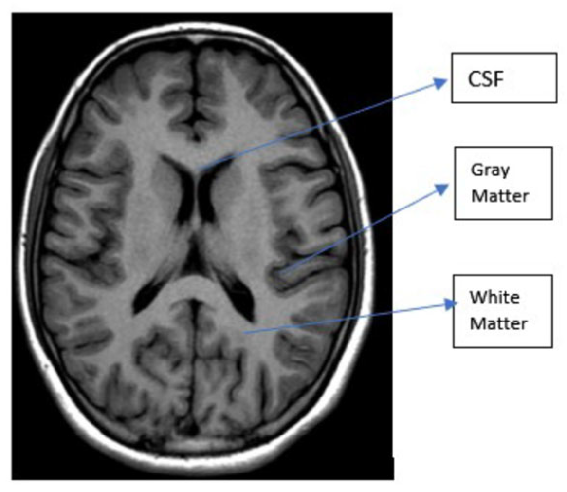
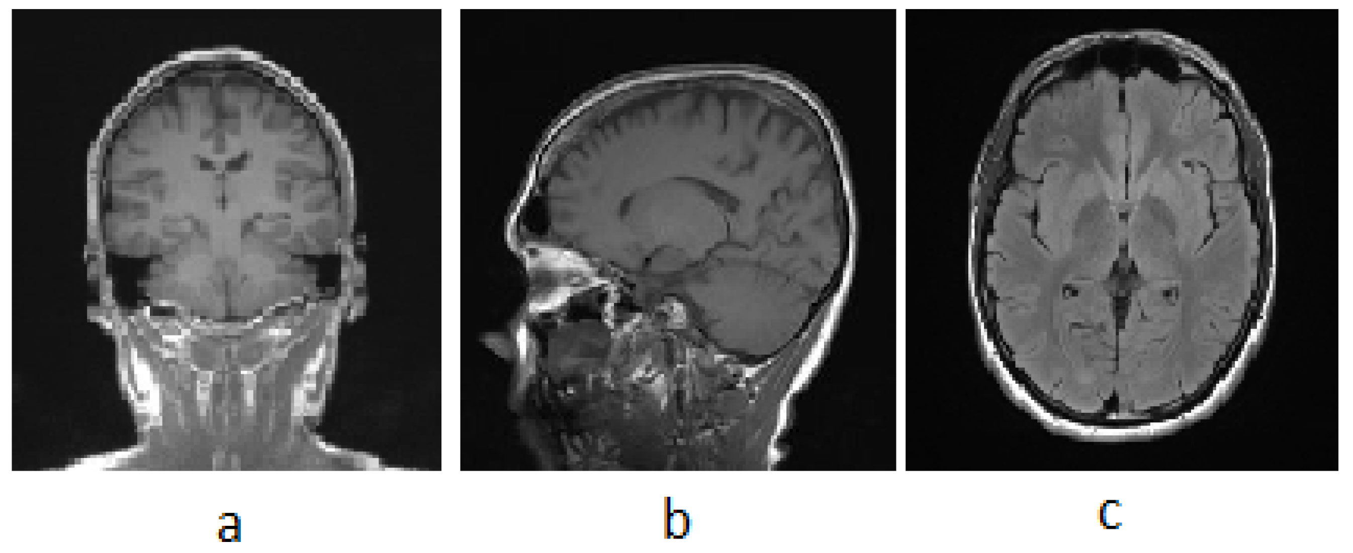
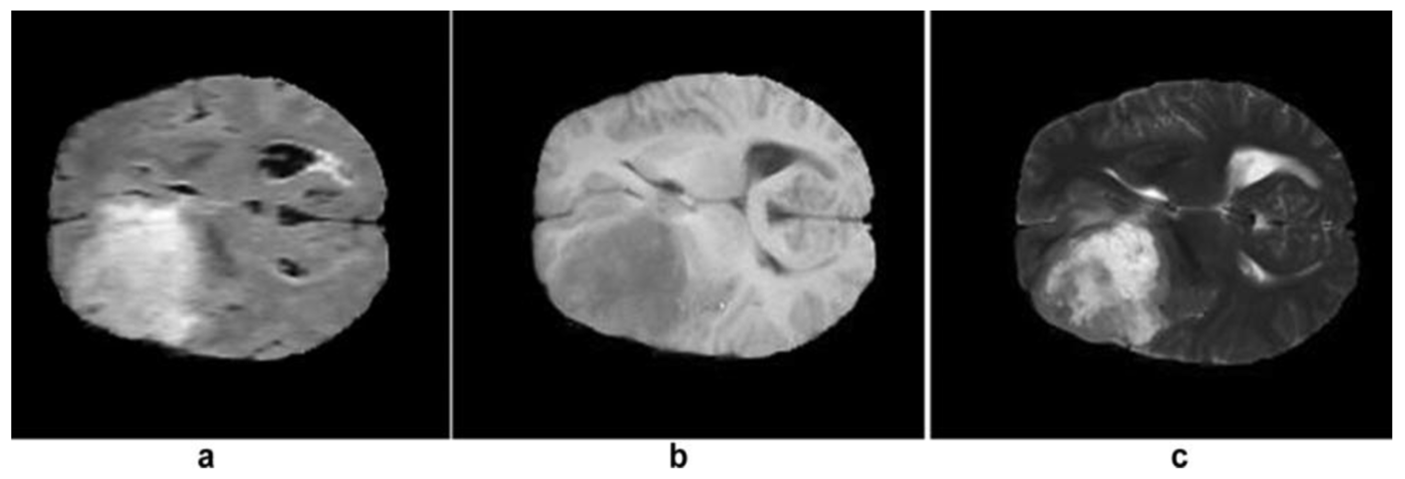
3.1. MRI
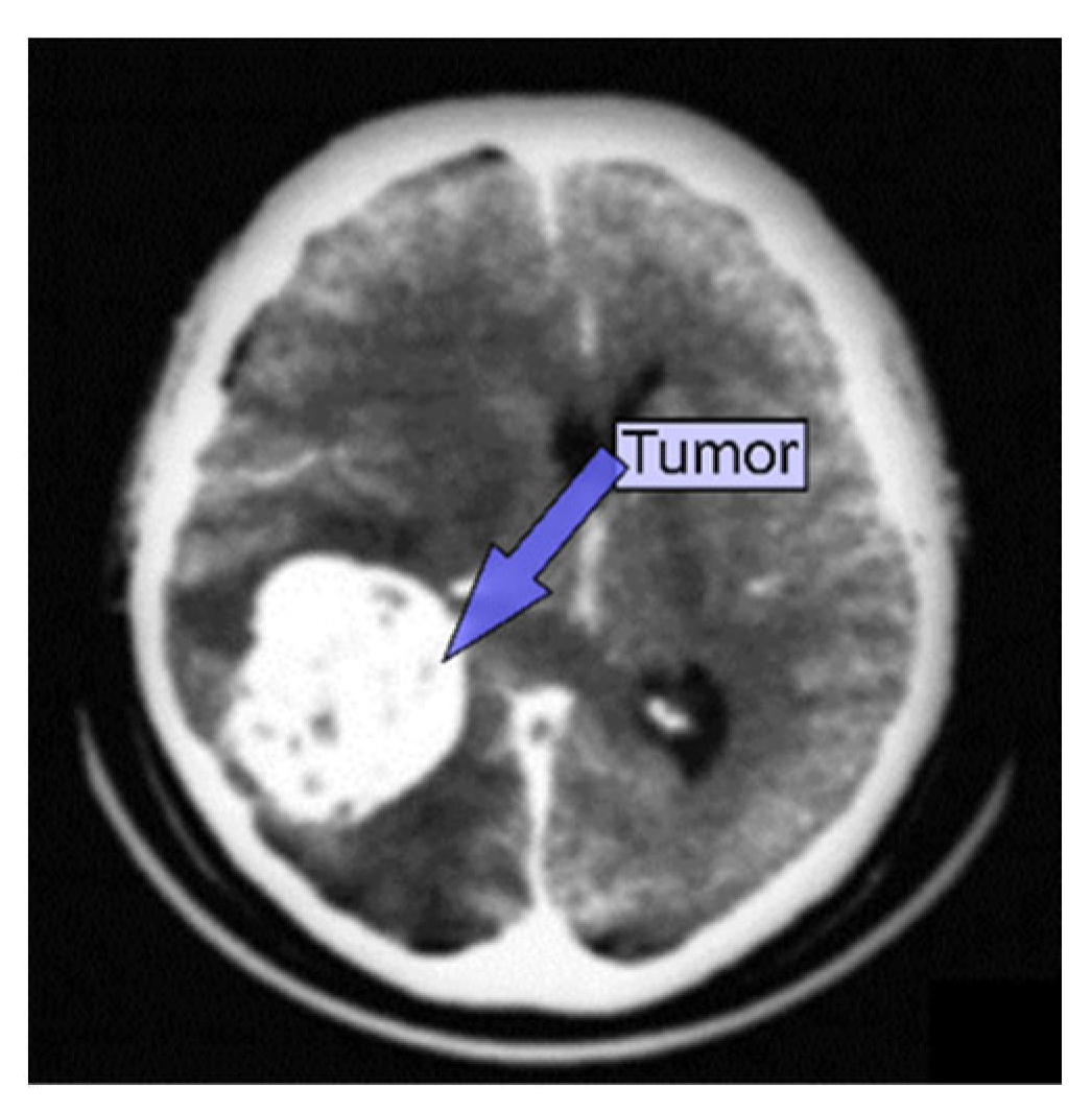
3.2. CT
3.3. PET
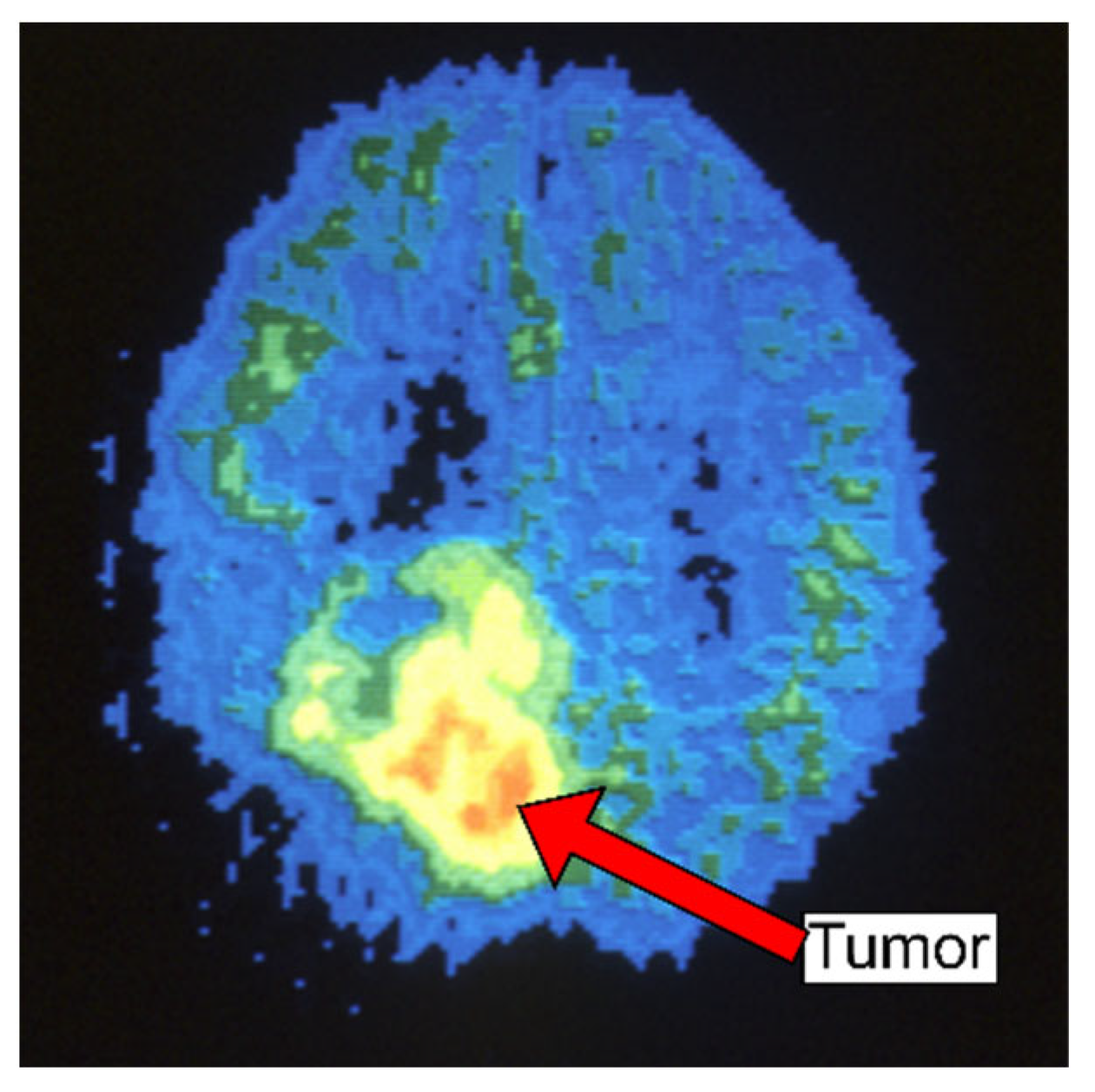
3.4. SPECT
3.5. Ultrasound
4. Classification and Segmentation Method
4.1. Classification Methods
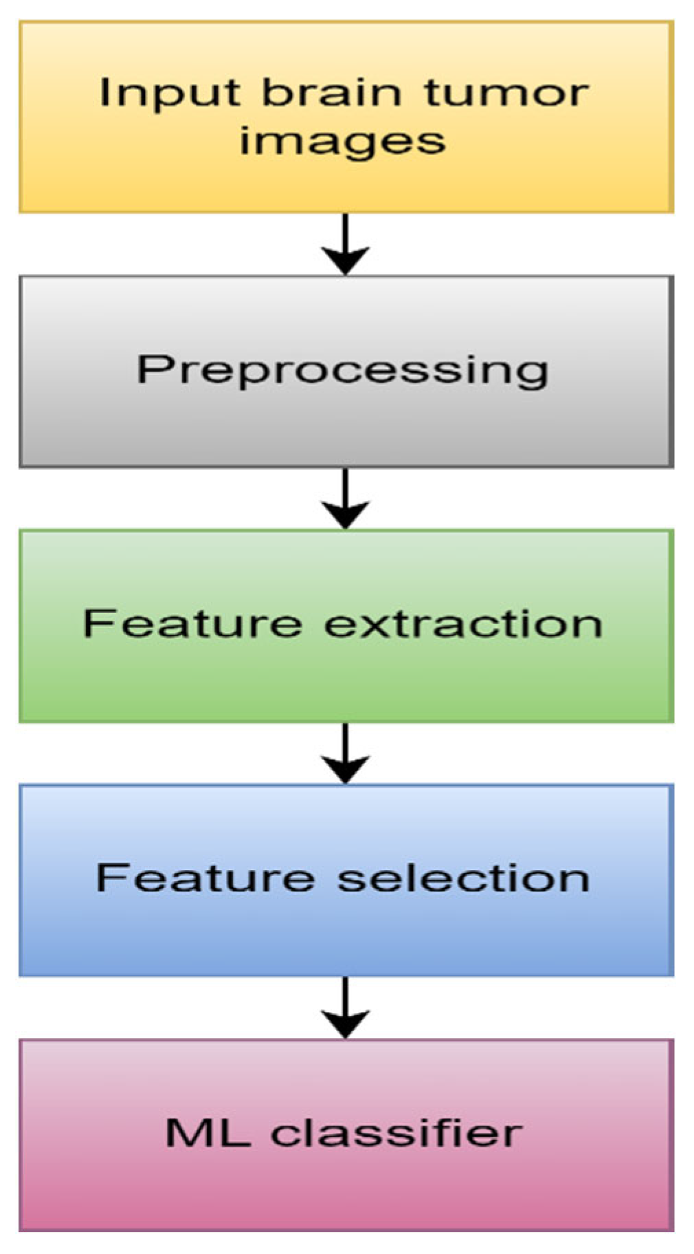
4.1.1. Machine Learning
- 1.
- Data Acquisition
- 2.
- Preprocessing
- 3.
- Feature extraction
- 4.
- Feature selection
- 5.
- ML algorithm
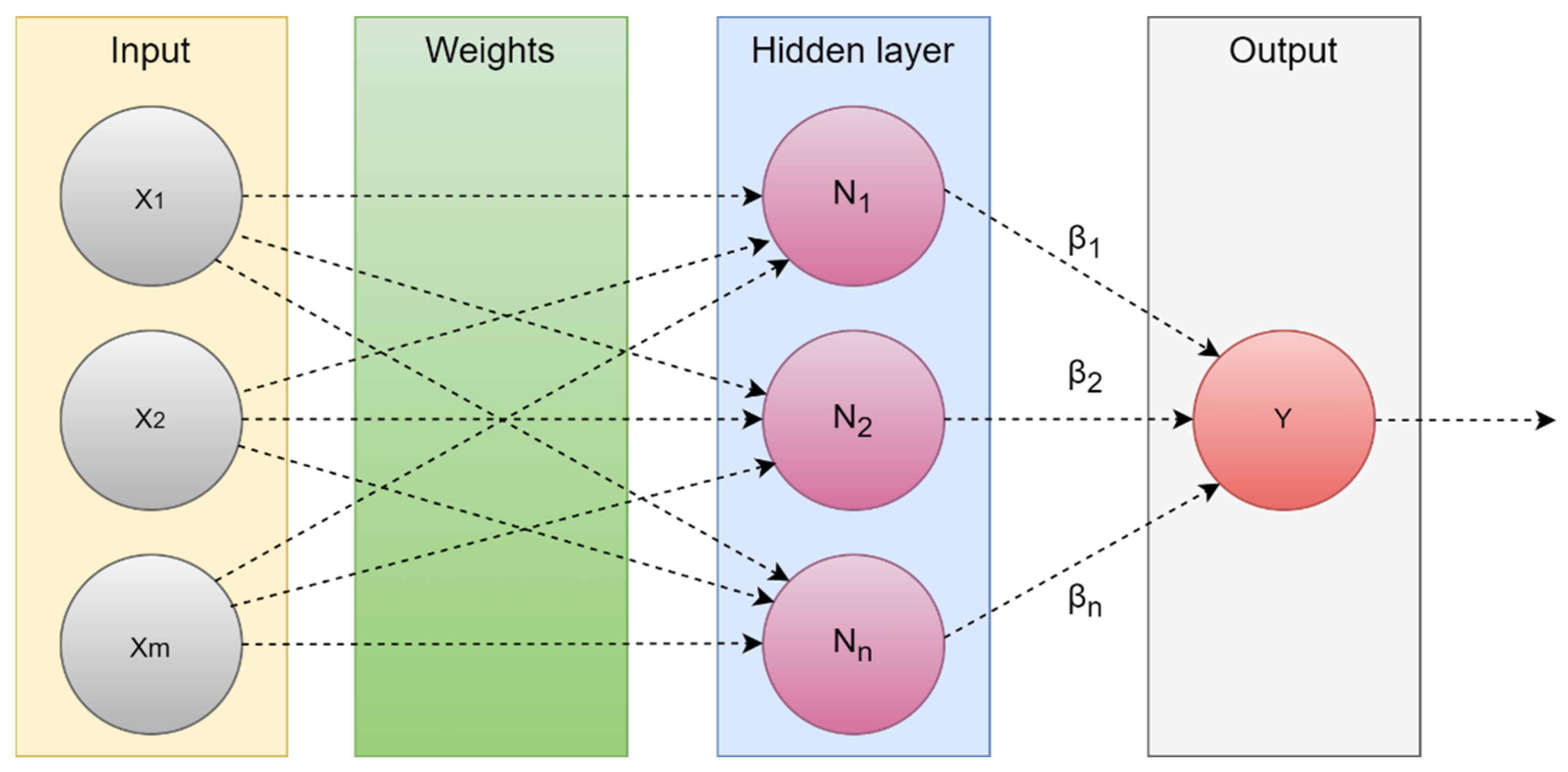
4.1.2. Extreme Learning Machine (ELM)
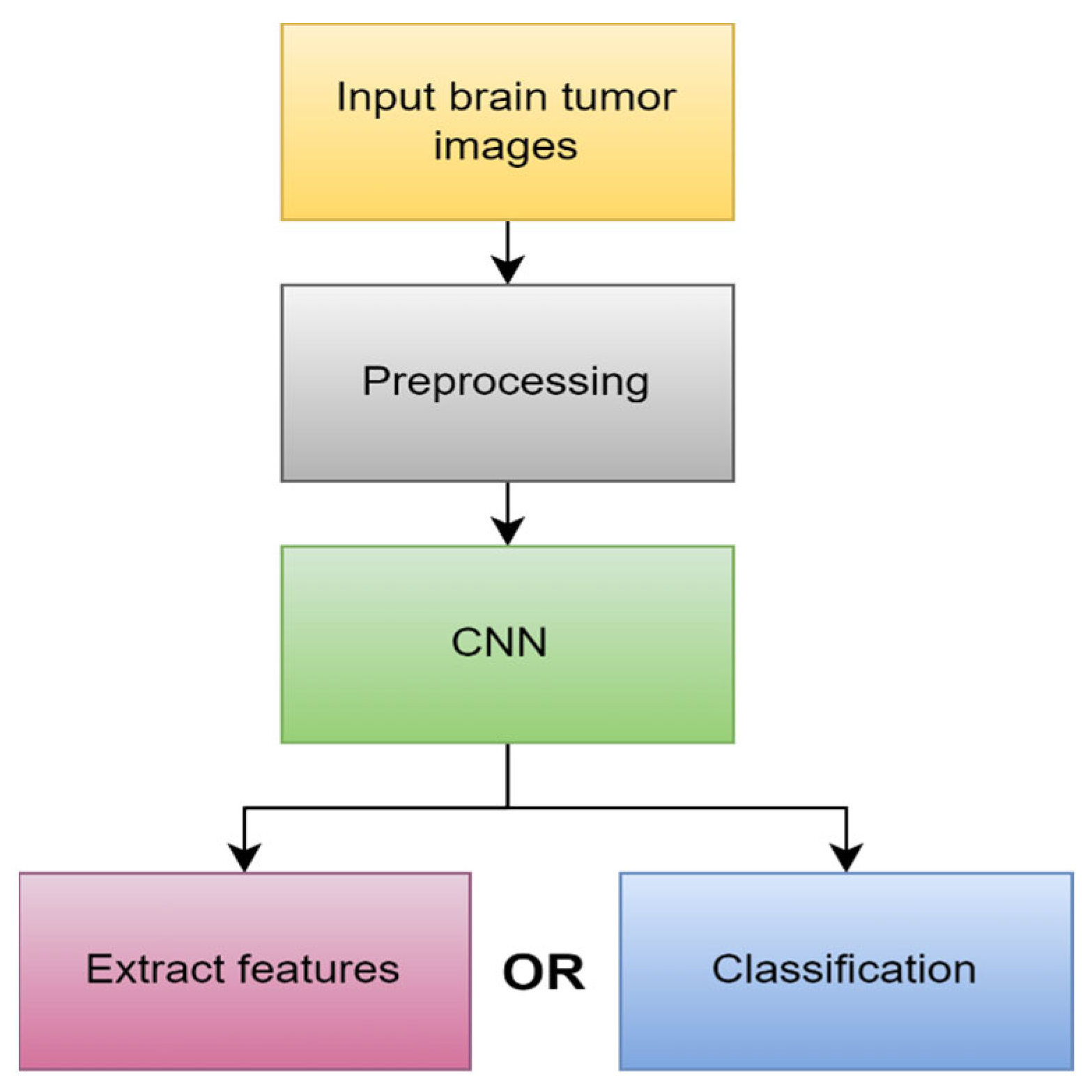
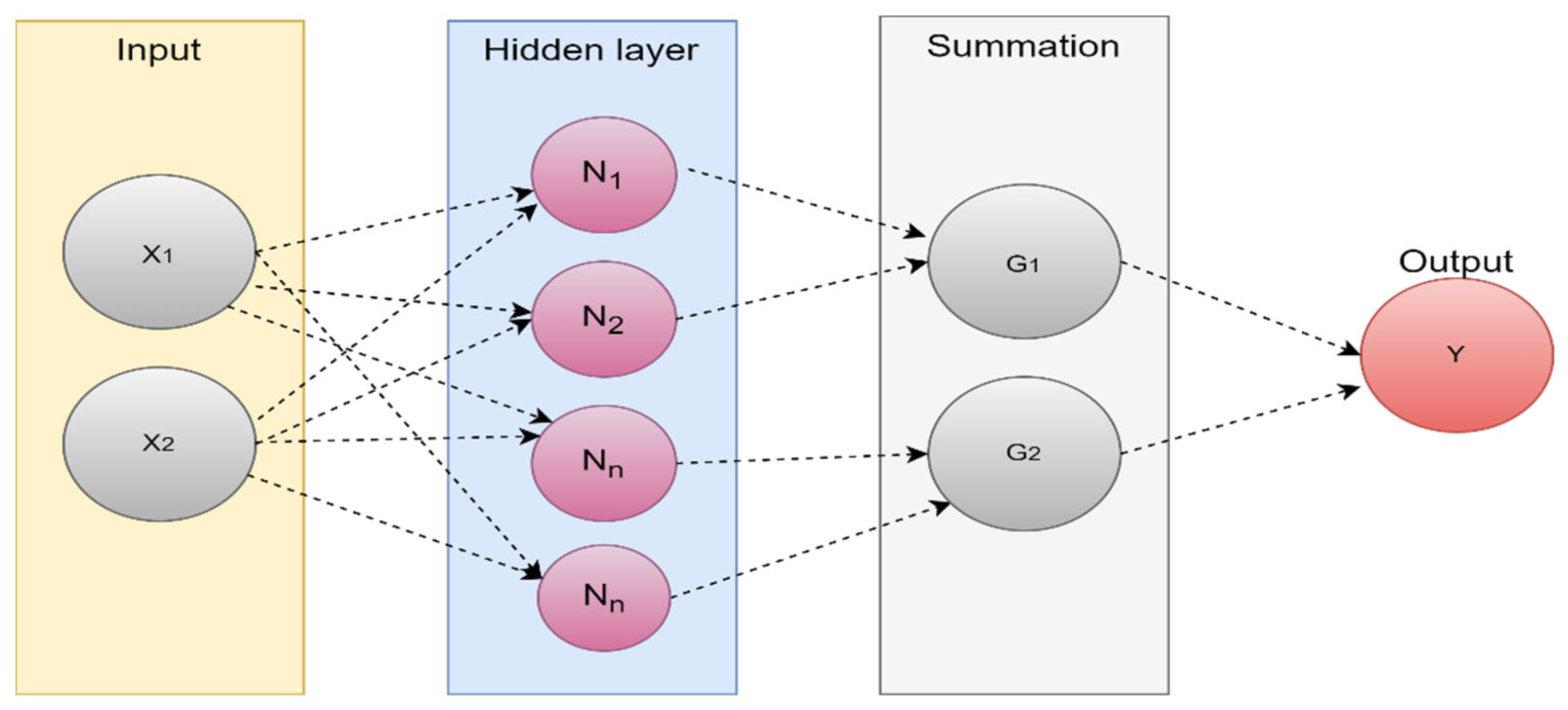
4.1.3. Deep Learning (DL)
4.2. Segmentation Method
4.2.1. Region-Based Segmentation
4.2.2. Thresholding Methods
4.2.3. Watershed Techniques
4.2.4. Morphological-Based Method
4.2.5. Edge-Based Method
4.2.6. Neural-Networks-Based Method
4.2.7. DL-Based Segmentation
4.3. Performance Evaluation
5. Literature Review
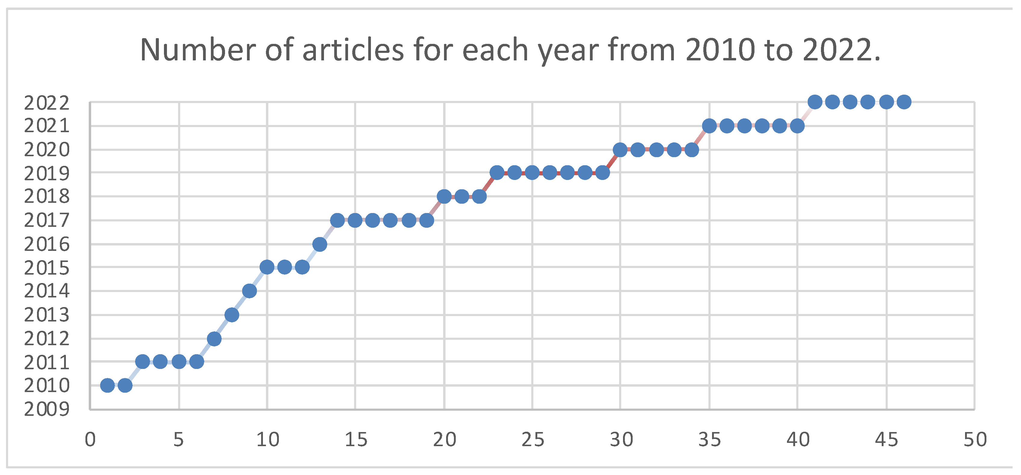
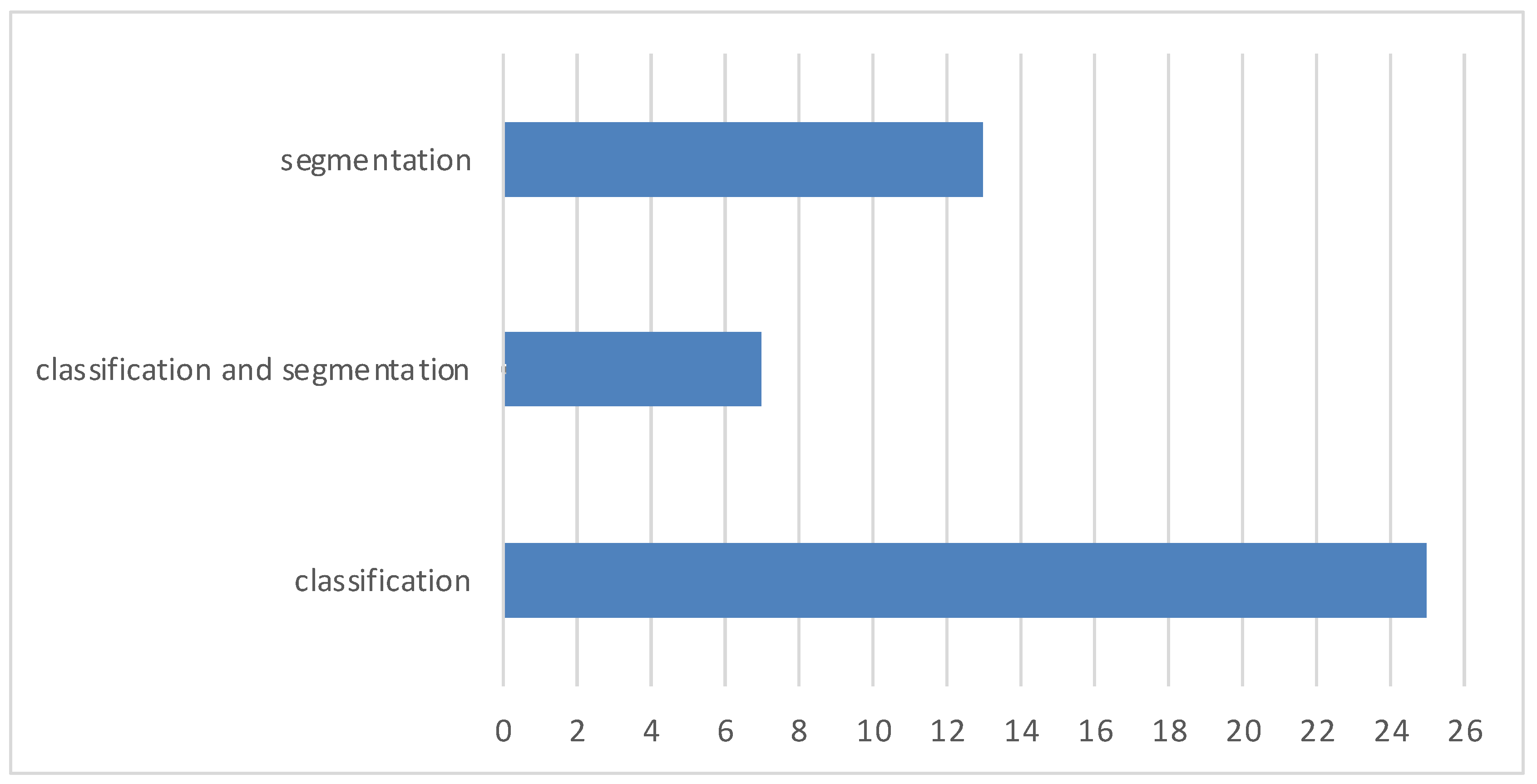
5.1. Article Selection
5.2. Publicly Available Datasets
5.3. Related Work
5.3.1. MRI Brain Tumor Segmentation
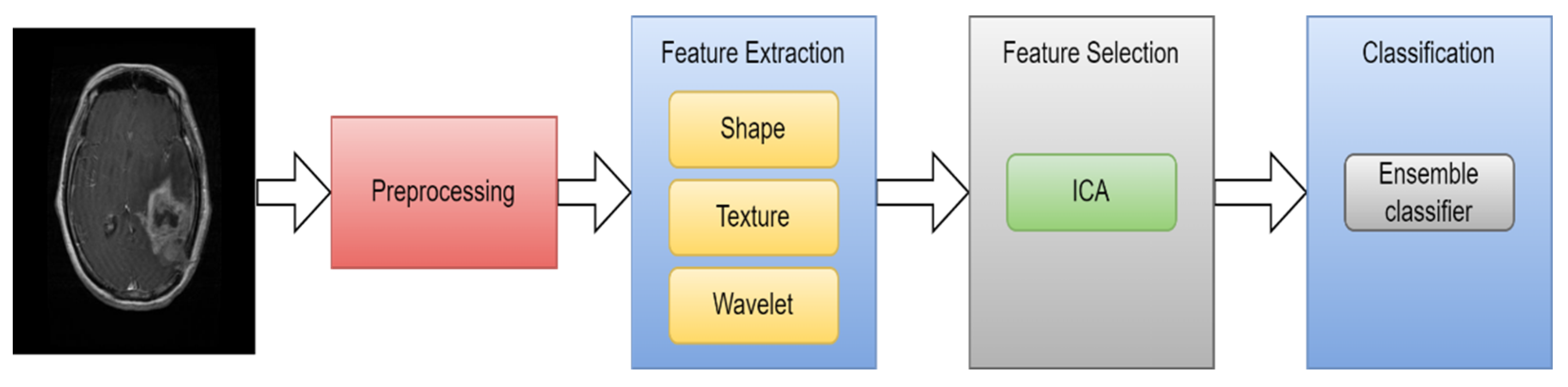
5.3.2. MRI Brain Tumor Classification Using ML

| Ref. | Scan | Year | Feature Extraction | Feature Selection | Classification | Acc. |
|---|---|---|---|---|---|---|
| [96] | MRI | 2010 | GLCM | PCA | ANN and KNN | 98% and 97% |
| [91] | MRI | 2011 | Wavelet | PCA | Back-propagation NN | 100.00% |
| [94] | MRI | 2013 | Intensity and texture | PCA | ANN | 85.50% |
| [95] | MRI | 2014 | GLCM | - | SVM | 93.00% |
| [36] | MRI | 2015 | Texture and shape | ICA | SVM | 99.09% |
| [92] | MRI | 2015 | Wavelet | - | SVM | 97.00% |
| [28] | MRI | 2017 | Texture and shape | - | SVM | 97.10% |
| [93] | MRI | 2017 | Intensity and texture | - | ANN | 92.43% |
| [97] | MRI | 2020 | DWT | Mean and standard deviation | DNN | 95.8% |
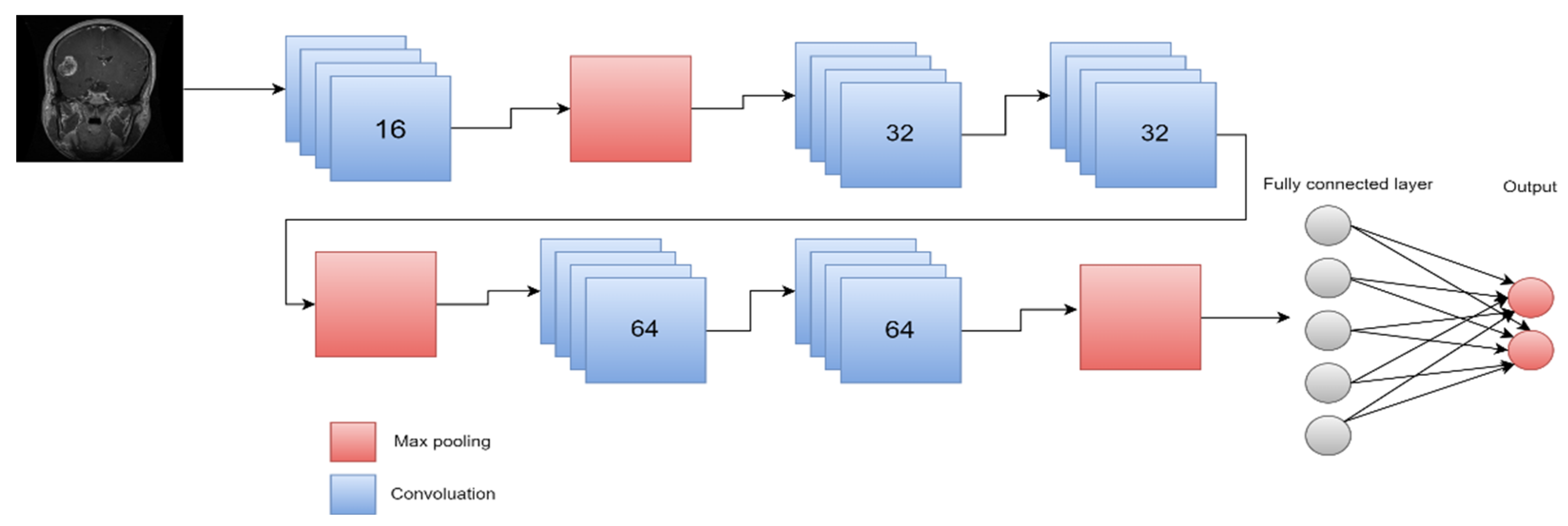
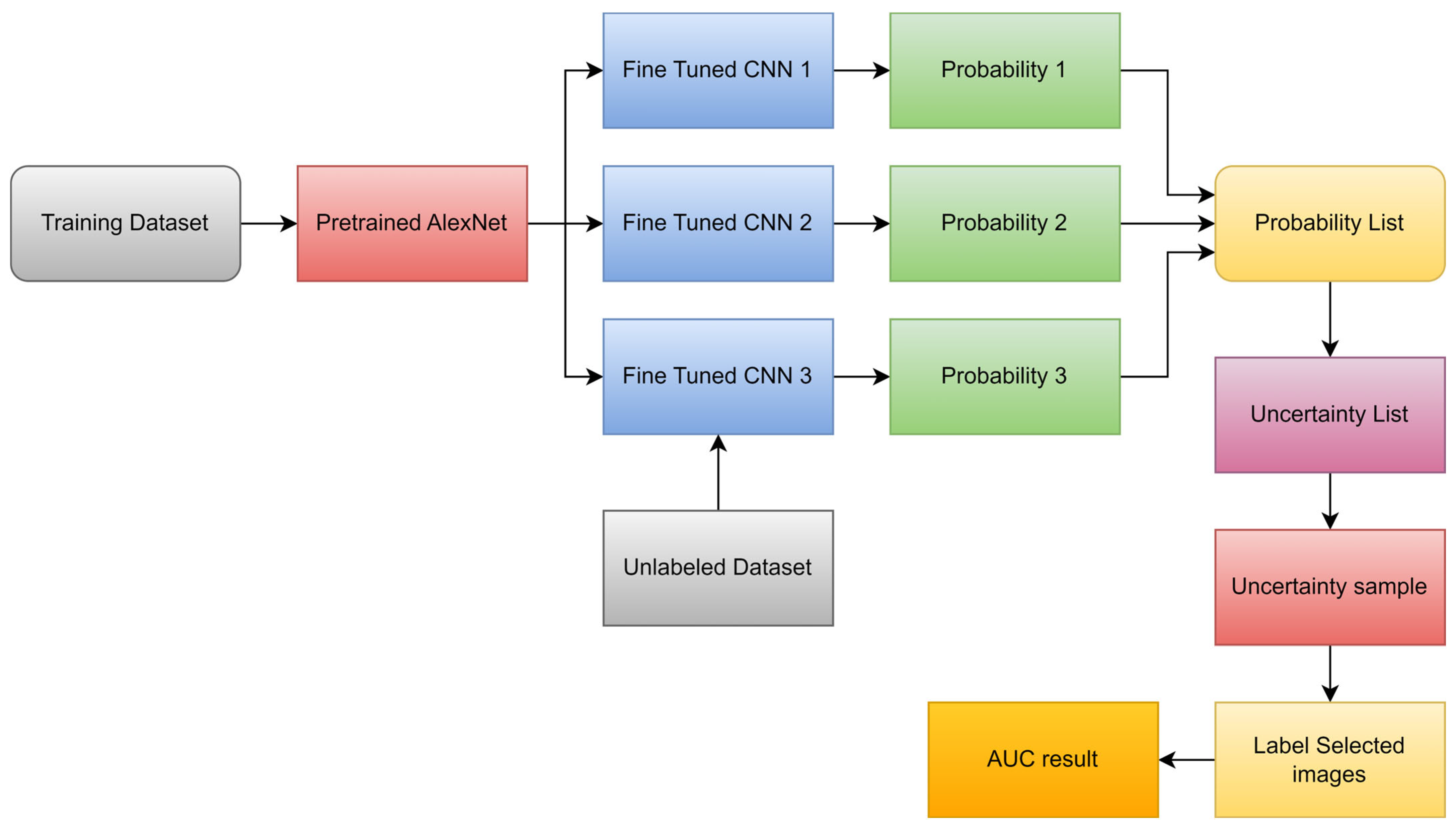
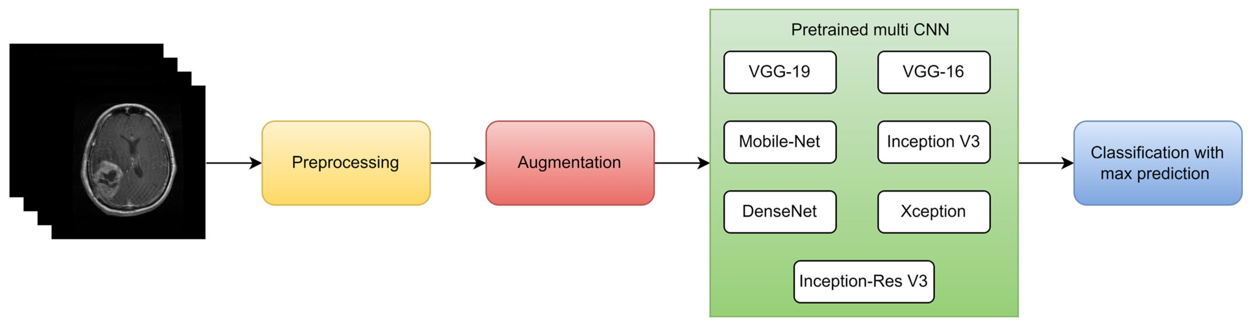
5.3.3. MRI Brain Tumor Classification Using DL
5.3.4. Hybrid Techniques
| Ref. | Year | Segmentation Method | Feature Extraction | Classifier | Accuracy |
|---|---|---|---|---|---|
| [115] | 2017 | FCM | shape and statistical | SVM and ANN | 97.44% and 97.37% |
| [118] | 2017 | FCM | DWT and PCA | CNN | 98.00% |
| [52] | 2019 | watershed | shape | KNN | 89.50% |
| [30] | 2019 | Ostu’s | DWT | SVM | 99.00% |
| [117] | 2020 | thresholding and watershed | CNN | SVM | 87.4%. |
| [116] | 2020 | canny | GLCM and Gabor | ANN | 98.90% |
| [119] | 2023 | thresholding | wavelet | CNN | 99.00% |
| [120] | 2023 | fuzzy clustering | GLCM | Improved SVM | 88.00% |
| [121] | 2023 | U-Net | DWT | CNN | 98.93% |
5.3.5. Various Segmentation and Classification Methods Employing CT Images
6. Discussion
7. General Problems and Challenges
7.1. Brain Cancer and Other Brain Disorders
7.1.1. Stroke
7.1.2. Alzheimer’s Disease
8. Future Directions
9. Conclusions
Funding
Institutional Review Board Statement
Conflicts of Interest
References
- Watson, C.; Kirkcaldie, M.; Paxinos, G. The Brain: An Introduction to Functional Neuroanatomy. 2010. Available online: http://ci.nii.ac.jp/ncid/BB04049625 (accessed on 22 May 2023).
- Jellinger, K.A. The Human Nervous System Structure and Function, 6th edn. Eur. J. Neurol. 2009, 16, e136. [Google Scholar] [CrossRef]
- DeAngelis, L.M. Brain tumors. N. Engl. J. Med. 2001, 344, 114–123. [Google Scholar] [CrossRef]
- Louis, D.N.; Perry, A.; Wesseling, P.; Brat, D.J.; Cree, I.A.; Figarella-Branger, D.; Hawkins, C.; Ng, H.K.; Pfister, S.M.; Reifenberger, G.; et al. The 2021 WHO Classification of Tumors of the Central Nervous System: A summary. Neuro-Oncology 2021, 23, 1231–1251. [Google Scholar] [CrossRef]
- Hayward, R.M.; Patronas, N.; Baker, E.H.; Vézina, G.; Albert, P.S.; Warren, K.E. Inter-observer variability in the measurement of diffuse intrinsic pontine gliomas. J. Neuro-Oncol. 2008, 90, 57–61. [Google Scholar] [CrossRef]
- Mahaley, M.S., Jr.; Mettlin, C.; Natarajan, N.; Laws, E.R., Jr.; Peace, B.B. National survey of patterns of care for brain-tumor patients. J. Neurosurg. 1989, 71, 826–836. [Google Scholar] [CrossRef] [PubMed]
- Sultan, H.H.; Salem, N.M.; Al-Atabany, W. Multi-Classification of Brain Tumor Images Using Deep Neural Network. IEEE Access 2019, 7, 69215–69225. [Google Scholar] [CrossRef]
- Johnson, D.R.; Guerin, J.B.; Giannini, C.; Morris, J.M.; Eckel, L.J.; Kaufmann, T.J. 2016 Updates to the WHO Brain Tumor Classification System: What the Radiologist Needs to Know. RadioGraphics 2017, 37, 2164–2180. [Google Scholar] [CrossRef] [PubMed]
- Buckner, J.C.; Brown, P.D.; O’Neill, B.P.; Meyer, F.B.; Wetmore, C.J.; Uhm, J.H. Central Nervous System Tumors. Mayo Clin. Proc. 2007, 82, 1271–1286. [Google Scholar] [CrossRef] [PubMed]
- World Health Organization: WHO, “Cancer”. July 2019. Available online: https://www.who.int/health-topics/cancer (accessed on 30 March 2022).
- Amyot, F.; Arciniegas, D.B.; Brazaitis, M.P.; Curley, K.C.; Diaz-Arrastia, R.; Gandjbakhche, A.; Herscovitch, P.; Hinds, S.R.; Manley, G.T.; Pacifico, A.; et al. A Review of the Effectiveness of Neuroimaging Modalities for the Detection of Traumatic Brain Injury. J. Neurotrauma 2015, 32, 1693–1721. [Google Scholar] [CrossRef]
- Pope, W.B. Brain metastases: Neuroimaging. Handb. Clin. Neurol. 2018, 149, 89–112. [Google Scholar] [CrossRef]
- Abd-Ellah, M.K.; Awad, A.I.; Khalaf, A.A.; Hamed, H.F. A review on brain tumor diagnosis from MRI images: Practical implications, key achievements, and lessons learned. Magn. Reson. Imaging 2019, 61, 300–318. [Google Scholar] [CrossRef] [PubMed]
- Ammari, S.; Pitre-Champagnat, S.; Dercle, L.; Chouzenoux, E.; Moalla, S.; Reuze, S.; Talbot, H.; Mokoyoko, T.; Hadchiti, J.; Diffetocq, S.; et al. Influence of Magnetic Field Strength on Magnetic Resonance Imaging Radiomics Features in Brain Imaging, an In Vitro and In Vivo Study. Front. Oncol. 2021, 10, 541663. [Google Scholar] [CrossRef] [PubMed]
- Sahoo, L.; Sarangi, L.; Dash, B.R.; Palo, H.K. Detection and Classification of Brain Tumor Using Magnetic Resonance Images. In Advances in Electrical Control and Signal Systems: Select Proceedings of AECSS, Bhubaneswar, India, 8–9 November 2019; Springer: Singapore, 2020; Volume 665, pp. 429–441. [Google Scholar] [CrossRef]
- Kaur, R.; Doegar, A. Localization and Classification of Brain Tumor using Machine Learning & Deep Learning Techniques. Int. J. Innov. Technol. Explor. Eng. 2019, 8, 59–66. [Google Scholar]
- The Radiology Assistant: Multiple Sclerosis 2.0. 1 December 2021. Available online: https://radiologyassistant.nl/neuroradiology/multiple-sclerosis/diagnosis-and-differential-diagnosis-3#mri-protocol-ms-brain-protocol (accessed on 22 May 2023).
- Savoy, R.L. Functional magnetic resonance imaging (fMRI). In Encyclopedia of Neuroscience; Elsevier: Charlestown, MA, USA, 1999. [Google Scholar]
- Luo, Q.; Li, Y.; Luo, L.; Diao, W. Comparisons of the accuracy of radiation diagnostic modalities in brain tumor. Medicine 2018, 97, e11256. [Google Scholar] [CrossRef]
- Positron Emission Tomography (PET). Johns Hopkins Medicine. 20 August 2021. Available online: https://www.hopkinsmedicine.org/health/treatment-tests-and-therapies/positron-emission-tomography-pet (accessed on 20 May 2023).
- Mayfield Brain and Spine. SPECT Scan. 2022. Available online: https://mayfieldclinic.com/pe-spect.htm (accessed on 22 May 2023).
- Sastry, R.; Bi, W.L.; Pieper, S.; Frisken, S.; Kapur, T.; Wells, W.; Golby, A.J. Applications of Ultrasound in the Resection of Brain Tumors. J. Neuroimaging 2016, 27, 5–15. [Google Scholar] [CrossRef]
- Nasrabadi, N.M. Pattern recognition and machine learning. J. Electron. Imaging 2007, 16, 49901. [Google Scholar]
- Erickson, B.J.; Korfiatis, P.; Akkus, Z.; Kline, T.L. Machine learning for medical imaging. Radiographics 2017, 37, 505–515. [Google Scholar] [CrossRef]
- Mohan, M.R.M.; Sulochana, C.H.; Latha, T. Medical image denoising using multistage directional median filter. In Proceedings of the 2015 International Conference on Circuits, Power and Computing Technologies [ICCPCT-2015], Nagercoil, India, 9–20 March 2015. [Google Scholar]
- Borole, V.Y.; Nimbhore, S.S.; Kawthekar, S.S. Image processing techniques for brain tumor detection: A review. Int. J. Emerg. Trends Technol. Comput. Sci. (IJETTCS) 2015, 4, 2. [Google Scholar]
- Ziedan, R.H.; Mead, M.A.; Eltawel, G.S. Selecting the Appropriate Feature Extraction Techniques for Automatic Medical Images Classification. Int. J. 2016, 4, 1–9. [Google Scholar]
- Amin, J.; Sharif, M.; Yasmin, M.; Fernandes, S.L. A distinctive approach in brain tumor detection and classification using MRI. Pattern Recognit. Lett. 2017, 139, 118–127. [Google Scholar] [CrossRef]
- Islam, A.; Reza, S.M.; Iftekharuddin, K.M. Multifractal texture estimation for detection and segmentation of brain tumors. IEEE Trans. Biomed. Eng. 2013, 60, 3204–3215. [Google Scholar] [CrossRef]
- Gurbină, M.; Lascu, M.; Lascu, D. Tumor detection and classification of MRI brain image using different wavelet transforms and support vector machines. In Proceedings of the 2019 42nd International Conference on Telecommunications and Signal Processing (TSP), Budapest, Hungary, 1–3 July 2019; pp. 505–508. [Google Scholar]
- Xu, X.; Zhang, X.; Tian, Q.; Zhang, G.; Liu, Y.; Cui, G.; Meng, J.; Wu, Y.; Liu, T.; Yang, Z.; et al. Three-dimensional texture features from intensity and high-order derivative maps for the discrimination between bladder tumors and wall tissues via MRI. Int. J. Comput. Assist. Radiol. Surg. 2017, 12, 645–656. [Google Scholar] [CrossRef]
- Kaplan, K.; Kaya, Y.; Kuncan, M.; Ertunç, H.M. Brain tumor classification using modified local binary patterns (LBP) feature extraction methods. Med. Hypotheses 2020, 139, 109696. [Google Scholar] [CrossRef]
- Afza, F.; Khan, M.S.; Sharif, M.; Saba, T. Microscopic skin laceration segmentation and classification: A framework of statistical normal distribution and optimal feature selection. Microsc. Res. Tech. 2019, 82, 1471–1488. [Google Scholar] [CrossRef]
- Lakshmi, A.; Arivoli, T.; Rajasekaran, M.P. A Novel M-ACA-Based Tumor Segmentation and DAPP Feature Extraction with PPCSO-PKC-Based MRI Classification. Arab. J. Sci. Eng. 2017, 43, 7095–7111. [Google Scholar] [CrossRef]
- Adair, J.; Brownlee, A.; Ochoa, G. Evolutionary Algorithms with Linkage Information for Feature Selection in Brain Computer Interfaces. In Advances in Computational Intelligence Systems; Springer Nature: Cham, Switzerland, 2016; pp. 287–307. [Google Scholar]
- Arakeri, M.P.; Reddy, G.R.M. Computeraided diagnosis system for tissue characterization of brain tumor on magnetic resonance images. Signal Image Video Process. 2015, 9, 409–425. [Google Scholar] [CrossRef]
- Wang, S.; Zhang, Y.; Dong, Z.; Du, S.; Ji, G.; Yan, J.; Phillips, P. Feed-forward neural network optimized by hybridization of PSO and ABC for abnormal brain detection. Int. J. Imaging Syst. Technol. 2015, 25, 153–164. [Google Scholar] [CrossRef]
- Abbasi, S.; Tajeripour, F. Detection of brain tumor in 3D MRI images using local binary patterns and histogram orientation gradient. Neurocomputing 2017, 219, 526–535. [Google Scholar] [CrossRef]
- Zöllner, F.G.; Emblem, K.E.; Schad, L.R. SVM-based glioma grading: Optimization by feature reduction analysis. Z. Med. Phys. 2012, 22, 205–214. [Google Scholar] [CrossRef]
- Huang, G.-B.; Zhu, Q.-Y.; Siew, C.-K. Extreme learning machine: Theory and applications. Neurocomputing 2006, 70, 489–501. [Google Scholar] [CrossRef]
- Bhatele, K.R.; Bhadauria, S.S. Brain structural disorders detection and classification approaches: A review. Artif. Intell. Rev. 2019, 53, 3349–3401. [Google Scholar] [CrossRef]
- Schmidhuber, J. Deep Learning in Neural Networks: An Overview. Neural Netw. 2015, 61, 85–117. [Google Scholar] [CrossRef]
- Hu, A.; Razmjooy, N. Brain tumor diagnosis based on metaheuristics and deep learning. Int. J. Imaging Syst. Technol. 2020, 31, 657–669. [Google Scholar] [CrossRef]
- Tandel, G.S.; Balestrieri, A.; Jujaray, T.; Khanna, N.N.; Saba, L.; Suri, J.S. Multiclass magnetic resonance imaging brain tumor classification using artificial intelligence paradigm. Comput. Biol. Med. 2020, 122, 103804. [Google Scholar] [CrossRef] [PubMed]
- Sahaai, M.B. Brain tumor detection using DNN algorithm. Turk. J. Comput. Math. Educ. (TURCOMAT) 2021, 12, 3338–3345. [Google Scholar]
- Hashemi, M. Enlarging smaller images before inputting into convolutional neural network: Zero-padding vs. interpolation. J. Big Data 2019, 6, 98. [Google Scholar] [CrossRef]
- Miotto, R.; Wang, F.; Wang, S.; Jiang, X.; Dudley, J.T. Deep learning for healthcare: Review, opportunities and challenges. Briefings Bioinform. 2017, 19, 1236–1246. [Google Scholar] [CrossRef]
- Gorach, T. Deep convolutional neural networks—A review. Int. Res. J. Eng. Technol. (IRJET) 2018, 5, 439. [Google Scholar]
- Ogundokun, R.O.; Maskeliunas, R.; Misra, S.; Damaševičius, R. Improved CNN Based on Batch Normalization and Adam Optimizer. In Proceedings of the Computational Science and Its Applications–ICCSA 2022 Workshops, Malaga, Spain, 4–7 July 2022; Part V. pp. 593–604. [Google Scholar]
- Ismael SA, A.; Mohammed, A.; Hefny, H. An enhanced deep learning approach for brain cancer MRI images classification using residual networks. Artif. Intell. Med. 2020, 102, 101779. [Google Scholar] [CrossRef]
- Baheti, P. A Comprehensive Guide to Convolutional Neural Networks. V7. Available online: https://www.v7labs.com/blog/convolutional-neural-networks-guide (accessed on 24 April 2023).
- Ramdlon, R.H.; Kusumaningtyas, E.M.; Karlita, T. Brain Tumor Classification Using MRI Images with K-Nearest Neighbor Method. In Proceedings of the 2019 International Electronics Symposium (IES), Surabaya, Indonesia, 27–28 September 2019; pp. 660–667. [Google Scholar] [CrossRef]
- Gurusamy, R.; Subramaniam, V. A machine learning approach for MRI brain tumor classification. Comput. Mater. Contin. 2017, 53, 91–109. [Google Scholar]
- Pohle, R.; Toennies, K.D. Segmentation of medical images using adaptive region growing. In Proceedings of the Medical Imaging 2001: Image Processing, San Diego, CA, USA, 4–10 November 2001; Volume 4322, pp. 1337–1346. [Google Scholar] [CrossRef]
- Dey, N.; Ashour, A.S. Computing in medical image analysis. In Soft Computing Based Medical Image Analysis; Academic Press: Cambridge, MA, USA, 2018; pp. 3–11. [Google Scholar]
- Hooda, H.; Verma, O.P.; Singhal, T. Brain tumor segmentation: A performance analysis using K-Means, Fuzzy C-Means and Region growing algorithm. In Proceedings of the 2014 IEEE International Conference on Advanced Communications, Control and Computing Technologies, Ramanathapuram, India, 8–10 May 2014; pp. 1621–1626. [Google Scholar]
- Sharif, M.; Tanvir, U.; Munir, E.U.; Khan, M.A.; Yasmin, M. Brain tumor segmentation and classification by improved binomial thresholding and multi-features selection. J. Ambient. Intell. Humaniz. Comput. 2018, 1–20. [Google Scholar] [CrossRef]
- Shanthi, K.J.; Kumar, M.S. Skull stripping and automatic segmentation of brain MRI using seed growth and threshold techniques. In Proceedings of the 2007 International Conference on Intelligent and Advanced Systems, Kuala Lumpur, Malaysia, 25–28 November 2007; pp. 422–426. [Google Scholar] [CrossRef]
- Zhang, F.; Hancock, E.R. New Riemannian techniques for directional and tensorial image data. Pattern Recognit. 2010, 43, 1590–1606. [Google Scholar] [CrossRef]
- Singh, N.P.; Dixit, S.; Akshaya, A.S.; Khodanpur, B.I. Gradient Magnitude Based Watershed Segmentation for Brain Tumor Segmentation and Classification. In Advances in Intelligent Systems and Computing; Springer Nature: Cham, Switzerland, 2017; pp. 611–619. [Google Scholar] [CrossRef]
- Couprie, M.; Bertrand, G. Topological gray-scale watershed transformation. Vis. Geom. VI 1997, 3168, 136–146. [Google Scholar] [CrossRef]
- Khan, M.S.; Lali, M.I.U.; Saba, T.; Ishaq, M.; Sharif, M.; Saba, T.; Zahoor, S.; Akram, T. Brain tumor detection and classification: A framework of marker-based watershed algorithm and multilevel priority features selection. Microsc. Res. Tech. 2019, 82, 909–922. [Google Scholar] [CrossRef]
- Lotufo, R.; Falcao, A.; Zampirolli, F. IFT-Watershed from gray-scale marker. In Proceedings of the XV Brazilian Symposium on Computer Graphics and Image Processing, Fortaleza, Brazil, 10 October 2003. [Google Scholar] [CrossRef]
- Dougherty, E.R. An Introduction to Morphological Image Processing; SPIE Optical Engineering Press: Bellingham, WA, USA, 1992. [Google Scholar]
- Kaur, D.; Kaur, Y. Various image segmentation techniques: A review. Int. J. Comput. Sci. Mob. Comput. 2014, 3, 809–814. [Google Scholar]
- Aslam, A.; Khan, E.; Beg, M.S. Improved Edge Detection Algorithm for Brain Tumor Segmentation. Procedia Comput. Sci. 2015, 58, 430–437. [Google Scholar] [CrossRef]
- Egmont-Petersen, M.; de Ridder, D.; Handels, H. Image processing with neural networks—A review. Pattern Recognit. 2002, 35, 2279–2301. [Google Scholar] [CrossRef]
- Cui, B.; Xie, M.; Wang, C. A Deep Convolutional Neural Network Learning Transfer to SVM-Based Segmentation Method for Brain Tumor. In Proceedings of the 2019 IEEE 11th International Conference on Advanced Infocomm Technology (ICAIT), Jinan, China, 18–20 October 2019; pp. 1–5. [Google Scholar] [CrossRef]
- Pereira, S.; Pinto, A.; Alves, V.; Silva, C.A. Brain Tumor Segmentation Using Convolutional Neural Networks in MRI Images. IEEE Trans. Med. Imaging 2016, 35, 1240–1251. [Google Scholar] [CrossRef]
- Ye, N.; Yu, H.; Chen, Z.; Teng, C.; Liu, P.; Liu, X.; Xiong, Y.; Lin, X.; Li, S.; Li, X. Classification of Gliomas and Germinomas of the Basal Ganglia by Transfer Learning. Front. Oncol. 2022, 12, 844197. [Google Scholar] [CrossRef]
- Biratu, E.S.; Schwenker, F.; Ayano, Y.M.; Debelee, T.G. A survey of brain tumor segmentation and classification algorithms. J. Imaging 2021, 7, 179. [Google Scholar] [CrossRef]
- Wikipedia Contributors. F Score. Wikipedia. 2023. Available online: https://en.wikipedia.org/wiki/F-score (accessed on 22 May 2023).
- Brain Tumor Segmentation (BraTS) Challenge. Available online: http://www.braintumorsegmentation.org/ (accessed on 22 May 2023).
- RIDER NEURO MRI—The Cancer Imaging Archive (TCIA) Public Access—Cancer Imaging Archive Wiki. Available online: https://wiki.cancerimagingarchive.net/display/Public/RIDER+NEURO+MRI (accessed on 22 May 2023).
- Harvard Medical School Data. Available online: http://www.med.harvard.edu/AANLIB/ (accessed on 16 March 2021).
- The Cancer Genome Atlas. TCGA. Available online: https://wiki.cancerimagingarchive.net/display/Public/TCGA-GBM (accessed on 22 May 2023).
- The Cancer Genome Atlas. TCGA-LGG. Available online: https://wiki.cancerimagingarchive.net/display/Public/TCGA-LGG (accessed on 22 May 2023).
- Cheng, J. Figshare Brain Tumor Dataset. 2017. Available online: https://figshare.com/articles/dataset/brain_tumor_dataset/1512427/5 (accessed on 13 May 2022).
- IXI Dataset—Brain Development. Available online: https://brain-development.org/ixi-dataset/ (accessed on 22 May 2023).
- Gordillo, N.; Montseny, E.; Sobrevilla, P. A new fuzzy approach to brain tumor segmentation. In Proceedings of the 2010 IEEE International Conference, Barcelona, Spain, 18–23 July 2010; pp. 1–8. [Google Scholar] [CrossRef]
- Rajendran; Dhanasekaran, R. A hybrid Method Based on Fuzzy Clustering and Active Contour Using GGVF for Brain Tumor Segmentation on MRI Images. Eur. J. Sci. Res. 2011, 61, 305–313. [Google Scholar]
- Reddy, K.K.; Solmaz, B.; Yan, P.; Avgeropoulos, N.G.; Rippe, D.J.; Shah, M. Confidence guided enhancing brain tumor segmentation in multi-parametric MRI. In Proceedings of the 9th IEEE International Symposium on Biomedical Imaging, Barcelona, Spain, 2–5 May 2012; pp. 366–369. [Google Scholar] [CrossRef]
- Almahfud, M.A.; Setyawan, R.; Sari, C.A.; Setiadi, D.R.I.M.; Rachmawanto, E.H. An Effective MRI Brain Image Segmentation using Joint Clustering (K-Means and Fuzzy C-Means). In Proceedings of the 2018 International Seminar on Research of Information Technology and Intelligent Systems (ISRITI), Yogyakarta, Indonesia, 21–22 November 2018; pp. 11–16. [Google Scholar]
- Chen, W.; Qiao, X.; Liu, B.; Qi, X.; Wang, R.; Wang, X. Automatic brain tumor segmentation based on features of separated local square. In Proceedings of the 2017 Chinese Automation Congress (CAC), Jinan, China, 20–22 October 2017. [Google Scholar]
- Gupta, N.; Mishra, S.; Khanna, P. Glioma identification from brain MRI using superpixels and FCM clustering. In Proceedings of the 2018 Conference on Information and Communication Technology (CICT), Jabalpur, India, 26–28 October 2018. [Google Scholar] [CrossRef]
- Razzak, M.I.; Imran, M.; Xu, G. Efficient Brain Tumor Segmentation with Multiscale Two-Pathway-Group Conventional Neural Networks. IEEE J. Biomed. Health Inform. 2018, 23, 1911–1919. [Google Scholar] [CrossRef] [PubMed]
- Myronenko, A.; Hatamizadeh, A. Robust Semantic Segmentation of Brain Tumor Regions from 3D MRIs. In Proceedings of the International MICCAI Brainlesion Workshop, Singapore, 18 September 2020; pp. 82–89. [Google Scholar] [CrossRef]
- Karayegen, G.; Aksahin, M.F. Brain tumor prediction on MR images with semantic segmentation by using deep learning network and 3D imaging of tumor region. Biomed. Signal Process. Control. 2021, 66, 102458. [Google Scholar] [CrossRef]
- Ullah, Z.; Usman, M.; Jeon, M.; Gwak, J. Cascade multiscale residual attention CNNs with adaptive ROI for automatic brain tumor segmentation. Inf. Sci. 2022, 608, 1541–1556. [Google Scholar] [CrossRef]
- Wisaeng, K.; Sa-Ngiamvibool, W. Brain Tumor Segmentation Using Fuzzy Otsu Threshold Morphological Algorithm. IAENG Int. J. Appl. Math. 2023, 53, 1–12. [Google Scholar]
- Zhang, Y.; Dong, Z.; Wu, L.; Wang, S. A hybrid method for MRI brain image classification. Expert Syst. Appl. 2011, 38, 10049–10053. [Google Scholar] [CrossRef]
- Yang, G.; Zhang, Y.; Yang, J.; Ji, G.; Dong, Z.; Wang, S.; Feng, C.; Wang, Q. Automated classification of brain images using wavelet-energy and biogeography-based optimization. Multimed. Tools Appl. 2015, 75, 15601–15617. [Google Scholar] [CrossRef]
- Tiwari, P.; Sachdeva, J.; Ahuja, C.K.; Khandelwal, N. Computer Aided Diagnosis System—A Decision Support System for Clinical Diagnosis of Brain Tumours. Int. J. Comput. Intell. Syst. 2017, 10, 104–119. [Google Scholar] [CrossRef]
- Sachdeva, J.; Kumar, V.; Gupta, I.; Khandelwal, N.; Ahuja, C.K. Segmentation, Feature Extraction, and Multiclass Brain Tumor Classification. J. Digit. Imaging 2013, 26, 1141–1150. [Google Scholar] [CrossRef]
- Jayachandran, A.; Dhanasekaran, R. Severity Analysis of Brain Tumor in MRI Images Using Modified Multitexton Structure Descriptor and Kernel-SVM. Arab. J. Sci. Eng. 2014, 39, 7073–7086. [Google Scholar] [CrossRef]
- El-Dahshan, E.-S.A.; Hosny, T.; Salem, A.-B.M. Hybrid intelligent techniques for MRI brain images classification. Digit. Signal Process. 2010, 20, 433–441. [Google Scholar] [CrossRef]
- Ullah, Z.; Farooq, M.U.; Lee, S.-H.; An, D. A hybrid image enhancement based brain MRI images classification technique. Med. Hypotheses 2020, 143, 109922. [Google Scholar] [CrossRef] [PubMed]
- Kang, J.; Ullah, Z.; Gwak, J. MRI-Based Brain Tumor Classification Using Ensemble of Deep Features and Machine Learning Classifiers. Sensors 2021, 21, 2222. [Google Scholar] [CrossRef]
- Díaz-Pernas, F.; Martínez-Zarzuela, M.; Antón-Rodríguez, M.; González-Ortega, D. A Deep Learning Approach for Brain Tumor Classification and Segmentation Using a Multiscale Convolutional Neural Network. Healthcare 2021, 9, 153. [Google Scholar] [CrossRef] [PubMed]
- Badža, M.M.; Barjaktarović, M. Classification of Brain Tumors from MRI Images Using a Convolutional Neural Network. Appl. Sci. 2020, 10, 1999. [Google Scholar] [CrossRef]
- Ertosun, M.G.; Rubin, D.L. Automated Grading of Gliomas using Deep Learning in Digital Pathology Images: A modular approach with ensemble of convolutional neural networks. In Proceedings of the AMIA Annual Symposium, San Francisco, CA, USA, 14–18 November 2015; Volume 2015, pp. 1899–1908. [Google Scholar]
- Khan, H.A.; Jue, W.; Mushtaq, M.; Mushtaq, M.U. Brain tumor classification in MRI image using convolutional neural network. Math. Biosci. Eng. 2020, 17, 6203–6216. [Google Scholar] [CrossRef]
- Özcan, H.; Emiroğlu, B.G.; Sabuncuoğlu, H.; Özdoğan, S.; Soyer, A.; Saygı, T. A comparative study for glioma classification using deep convolutional neural networks. Math. Biosci. Eng. MBE 2021, 18, 1550–1572. [Google Scholar] [CrossRef]
- Hao, R.; Namdar, K.; Liu, L.; Khalvati, F. A Transfer Learning–Based Active Learning Framework for Brain Tumor Classification. Front. Artif. Intell. 2021, 4, 635766. [Google Scholar] [CrossRef]
- Yang, Y.; Yan, L.-F.; Zhang, X.; Han, Y.; Nan, H.-Y.; Hu, Y.-C.; Hu, B.; Yan, S.-L.; Zhang, J.; Cheng, D.-L.; et al. Glioma Grading on Conventional MR Images: A Deep Learning Study with Transfer Learning. Front. Neurosci. 2018, 12, 804. [Google Scholar] [CrossRef]
- El Hamdaoui, H.; Benfares, A.; Boujraf, S.; Chaoui, N.E.H.; Alami, B.; Maaroufi, M.; Qjidaa, H. High precision brain tumor classification model based on deep transfer learning and stacking concepts. Indones. J. Electr. Eng. Comput. Sci. 2021, 24, 167–177. [Google Scholar] [CrossRef]
- Khazaee, Z.; Langarizadeh, M.; Ahmadabadi, M.E.S. Developing an Artificial Intelligence Model for Tumor Grading and Classification, Based on MRI Sequences of Human Brain Gliomas. Int. J. Cancer Manag. 2022, 15, e120638. [Google Scholar] [CrossRef]
- Amou, M.A.; Xia, K.; Kamhi, S.; Mouhafid, M. A Novel MRI Diagnosis Method for Brain Tumor Classification Based on CNN and Bayesian Optimization. Healthcare 2022, 10, 494. [Google Scholar] [CrossRef] [PubMed]
- Alanazi, M.; Ali, M.; Hussain, J.; Zafar, A.; Mohatram, M.; Irfan, M.; AlRuwaili, R.; Alruwaili, M.; Ali, N.T.; Albarrak, A.M. Brain Tumor/Mass Classification Framework Using Magnetic-Resonance-Imaging-Based Isolated and Developed Transfer Deep-Learning Model. Sensors 2022, 22, 372. [Google Scholar] [CrossRef] [PubMed]
- Rizwan, M.; Shabbir, A.; Javed, A.R.; Shabbr, M.; Baker, T.; Al-Jumeily, D. Brain Tumor and Glioma Grade Classification Using Gaussian Convolutional Neural Network. IEEE Access 2022, 10, 29731–29740. [Google Scholar] [CrossRef]
- Isunuri, B.V.; Kakarla, J. Three-class brain tumor classification from magnetic resonance images using separable convolution based neural network. Concurr. Comput. Pract. Exp. 2021, 34, e6541. [Google Scholar] [CrossRef]
- Kaur, T.; Gandhi, T.K. Deep convolutional neural networks with transfer learning for automated brain image classification. J. Mach. Vis. Appl. 2020, 31, 20. [Google Scholar] [CrossRef]
- Rehman, A.; Naz, S.; Razzak, M.I.; Akram, F.; Imran, M. A Deep Learning-Based Framework for Automatic Brain Tumors Classification Using Transfer Learning. Circuits Syst. Signal Process. 2019, 39, 757–775. [Google Scholar] [CrossRef]
- Deepa, S.; Janet, J.; Sumathi, S.; Ananth, J.P. Hybrid Optimization Algorithm Enabled Deep Learning Approach Brain Tumor Segmentation and Classification Using MRI. J. Digit. Imaging 2023, 36, 847–868. [Google Scholar] [CrossRef]
- Ahmmed, R.; Swakshar, A.S.; Hossain, M.F.; Rafiq, M.A. Classification of tumors and it stages in brain MRI using support vector machine and artificial neural network. In Proceedings of the 2017 International Conference on Electrical, Computer and Communication Engineering (ECCE), Cox’s Bazar, Bangladesh, 16–18 February 2017. [Google Scholar]
- Sathi, K.A.; Islam, S. Hybrid Feature Extraction Based Brain Tumor Classification using an Artificial Neural Network. In Proceedings of the 2020 IEEE 5th International Conference on Computing Communication and Automation (ICCCA), Greater Noida, India, 30–31 October 2020; pp. 155–160. [Google Scholar] [CrossRef]
- Islam, R.; Imran, S.; Ashikuzzaman; Khan, M.A. Detection and Classification of Brain Tumor Based on Multilevel Segmentation with Convolutional Neural Network. J. Biomed. Sci. Eng. 2020, 13, 45–53. [Google Scholar] [CrossRef]
- Mohsen, H.; El-Dahshan, E.A.; El-Horbaty, E.M.; Salem, A.M. Classification using deep learning neural networks for brain tumors. Future Comput. Inform. J. 2017, 3, 68–71. [Google Scholar] [CrossRef]
- Babu, P.A.; Rao, B.S.; Reddy, Y.V.B.; Kumar, G.R.; Rao, J.N.; Koduru, S.K.R. Optimized CNN-based Brain Tumor Segmentation and Classification using Artificial Bee Colony and Thresholding. Int. J. Comput. Commun. Control. 2023, 18, 577. [Google Scholar] [CrossRef]
- Ansari, A.S. Numerical Simulation and Development of Brain Tumor Segmentation and Classification of Brain Tumor Using Improved Support Vector Machine. Int. J. Intell. Syst. Appl. Eng. 2023, 11, 35–44. [Google Scholar]
- Farajzadeh, N.; Sadeghzadeh, N.; Hashemzadeh, M. Brain tumor segmentation and classification on MRI via deep hybrid representation learning. Expert Syst. Appl. 2023, 224, 119963. [Google Scholar] [CrossRef]
- Padma, A.; Sukanesh, R. A wavelet based automatic segmentation of brain tumor in CT images using optimal statistical texture features. Int. J. Image Process. 2011, 5, 552–563. [Google Scholar]
- Padma, A.; Sukanesh, R. Automatic Classification and Segmentation of Brain Tumor in CT Images using Optimal Dominant Gray level Run length Texture Features. Int. J. Adv. Comput. Sci. Appl. 2011, 2, 53–121. [Google Scholar] [CrossRef]
- Ruba, T.; Tamilselvi, R.; Beham, M.P.; Aparna, N. Accurate Classification and Detection of Brain Cancer Cells in MRI and CT Images using Nano Contrast Agents. Biomed. Pharmacol. J. 2020, 13, 1227–1237. [Google Scholar] [CrossRef]
- Woźniak, M.; Siłka, J.; Wieczorek, M.W. Deep neural network correlation learning mechanism for CT brain tumor detection. Neural Comput. Appl. 2021, 35, 14611–14626. [Google Scholar] [CrossRef]
- Nanmaran, R.; Srimathi, S.; Yamuna, G.; Thanigaivel, S.; Vickram, A.S.; Priya, A.K.; Karthick, A.; Karpagam, J.; Mohanavel, V.; Muhibbullah, M. Investigating the Role of Image Fusion in Brain Tumor Classification Models Based on Machine Learning Algorithm for Personalized Medicine. Comput. Math. Methods Med. 2022, 2022, 7137524. [Google Scholar] [CrossRef]
- Burns, A.; Iliffe, S. Alzheimer’s disease. BMJ 2009, 338, b158. [Google Scholar] [CrossRef]

| Types of Tumors Based on | Type | Comment |
|---|---|---|
| Nature | Benign | Less aggressive and grows slowly |
| Malignant | Life-threatening and rapidly expanding | |
| Origin | Primary tumor | Originates in the brain directly |
| Secondary tumor | This tumor develops in another area of the body like lung and breast before migrating to the brain | |
| Grading | Grade I | Basically, regular in shape, and they develop slowly |
| Grade II | Appear strange to the view and grow more slowly | |
| Grade III | These tumors grow more quickly than grade II cancers | |
| Grade IV | Reproduced with greater rate | |
| Progression stage | Stage 0 | Malignant but do not invade neighboring cells |
| Stage 1 | Malignant and quickly spreading | |
| Stage 2 | ||
| Stage 3 | ||
| Stage 4 | The malignancy invades every part of the body |
| T1 | T2 | Flair | |
|---|---|---|---|
| White Matter | Bright | Dark | Dark |
| Gray Matter | Gray | Dark | Dark |
| CSF | Dark | Bright | Dark |
| Tumor | Dark | Bright | Bright |
| Parameter | Equation |
|---|---|
| ACC | |
| SEN | |
| SPE | |
| PR | |
| F1_SCORE | |
| DCS | |
| Jaccard |
| Dataset | MRI Sequences | Source |
|---|---|---|
| BRATS | T1, T2, FLAIR | [73] |
| RIDER | T1, T2, FLAIR | [74] |
| Harvard | T2 | [75] |
| TCGA | T1, T2, FLAIR | [76,77] |
| Figshare | T1 | [78] |
| IXI | T1, T2 | [79] |
| Ref. | Scan | Year | Technique | Method | Performance Metrics | Result |
|---|---|---|---|---|---|---|
| [80] | MRI | 2010 | region-based | FCM | Acc | 93.00% |
| [81] | MRI | 2011 | region-based | FCM | Jaccard | 83.19% |
| [82] | MRI | 2012 | NN | LBP with SVM | DSC | 69.00% |
| [69] | MRI | 2016 | DL | CNN | DSC | 88.00% |
| [84] | MRI | 2017 | NN | GLCM with SVM | DSC | 86.12% |
| [38] | MRI | 2017 | NN | LBP with RF | Jaccard and DSC | 87% and 93% |
| [85] | MRI | 2018 | region-based | FCM | Acc | 98.00% |
| [83] | MRI | 2018 | region-based | FCM and k-mean | Acc | 91.94% |
| [68] | MRI | 2019 | DL and NN | CNN with SVM | DSC | 88.00% |
| [86] | MRI | 2019 | DL | Two-path CNN | DSC | 89.20% |
| [87] | MRI | 2019 | DL | semantic | Acc | 88.20% |
| [88] | MRI | 2021 | DL | semantic | IoU | 91.72% |
| [89] | MRI | 2022 | DL | MRA-UNet | DSC | 98.18% |
| [90] | MRI | 2023 | region-based | Fuzzy Otsu Threshold | Acc | 94.37% |
| Ref. | Scan | Year | Technique | Method | Result | Performance Metrics |
|---|---|---|---|---|---|---|
| [101] | MRI | 2015 | DL | Custom-CNN | 96.00% | Acc |
| [7] | MRI | 2019 | DL | Custom-CNN | 98.70% | Acc |
| [102] | MRI | 2020 | DL | VGG-16, Inception-v3, ResNet-50 | 96% 75% 89% | Acc |
| [103] | MRI | 2021 | DL | AlexNet, GoogleNet, SqueezeNet | 97.10% | Acc |
| [104] | MRI | 2021 | DL | Custom-CNN | 82.89% | ROC |
| [105] | MRI | 2018 | DL | AlexNet | 90.90% | Test acc |
| [106] | MRI | 2021 | DL | multi-CNN structure | 98.67% 98.06% 98.33% 98.06% | precision, F1 score, precision, sensitivity |
| [107] | MRI | 2022 | DL | EfficientNetB0 | 98.80% | Acc |
| [70] | MRI | 2022 | DL | ResNet18 | 88.00% | AUC |
| [108] | MRI | 2022 | DL | Custom-CNN | 98.70% | Acc |
| [109] | MRI | 2022 | DL | Custom-CNN | 95.75% | Acc |
| [110] | MRI | 2022 | DL | Gaussian-CNN | 99.80% | Acc |
| [111] | MRI | 2020 | DL | seven-layer CNN | 97.52% | Acc |
| [112] | MRI | 2021 | DL | Alexnet | 100.00% | Acc |
| [113] | MRI | 2019 | DL | VGG16 | 98.69% | Acc |
| [114] | MRI | 2023 | DL | CNN | 92.10% | Acc |
| Ref. | Year | Type | Segmentation | Feature Extraction | Feature Selection | Classification | Result |
|---|---|---|---|---|---|---|---|
| [122] | 2011 | CT | NN | WCT and WST | GA | - | 97.00% |
| [123] | 2011 | CT | FCM and k-mean | GLCM and WCT | GA | SVM | 98.00% |
| [124] | 2020 | CT | Semantic | - | - | GoogleNet | 99.60% |
| [125] | 2021 | CT | - | - | - | CNN | 96.00% |
| [126] | 2022 | SPECT/MRI | - | DCT | - | SVM | 96.80% |
Disclaimer/Publisher’s Note: The statements, opinions and data contained in all publications are solely those of the individual author(s) and contributor(s) and not of MDPI and/or the editor(s). MDPI and/or the editor(s) disclaim responsibility for any injury to people or property resulting from any ideas, methods, instructions or products referred to in the content. |
© 2023 by the author. Licensee MDPI, Basel, Switzerland. This article is an open access article distributed under the terms and conditions of the Creative Commons Attribution (CC BY) license (https://creativecommons.org/licenses/by/4.0/).
Share and Cite
Kaifi, R. A Review of Recent Advances in Brain Tumor Diagnosis Based on AI-Based Classification. Diagnostics 2023, 13, 3007. https://doi.org/10.3390/diagnostics13183007
Kaifi R. A Review of Recent Advances in Brain Tumor Diagnosis Based on AI-Based Classification. Diagnostics. 2023; 13(18):3007. https://doi.org/10.3390/diagnostics13183007
Chicago/Turabian StyleKaifi, Reham. 2023. "A Review of Recent Advances in Brain Tumor Diagnosis Based on AI-Based Classification" Diagnostics 13, no. 18: 3007. https://doi.org/10.3390/diagnostics13183007
APA StyleKaifi, R. (2023). A Review of Recent Advances in Brain Tumor Diagnosis Based on AI-Based Classification. Diagnostics, 13(18), 3007. https://doi.org/10.3390/diagnostics13183007