
Semantic Segmentation of Extraocular Muscles on Computed Tomography Images Using Convolutional Neural Networks


Abstract
:1. Introduction
2. Materials and Methods
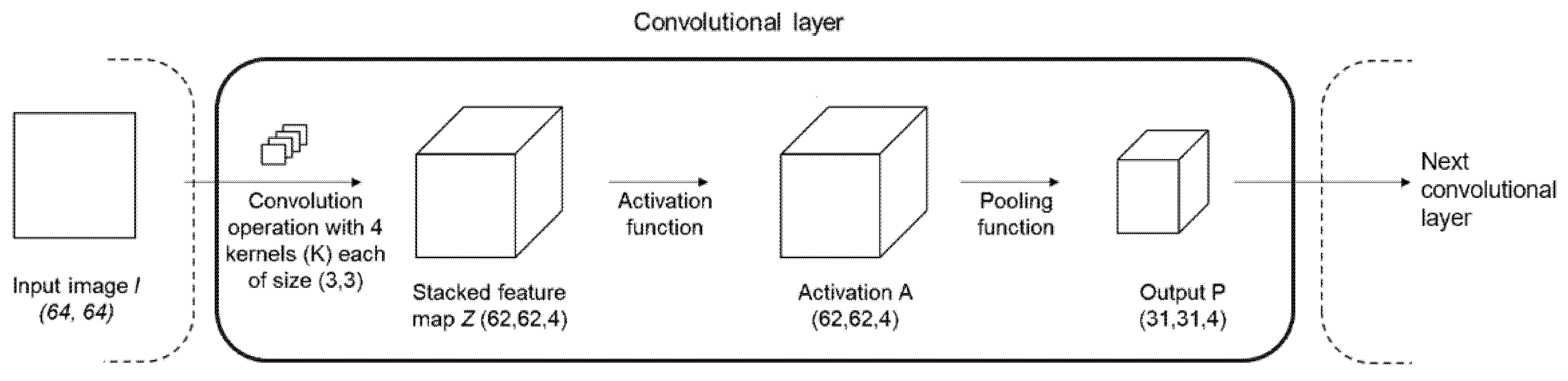
2.1. Convolutional Neural Network (CNN)
2.2. Dataset
2.3. Image Acquisition
2.4. Data Preprocessing
2.5. Architecture
2.6. Loss Functions
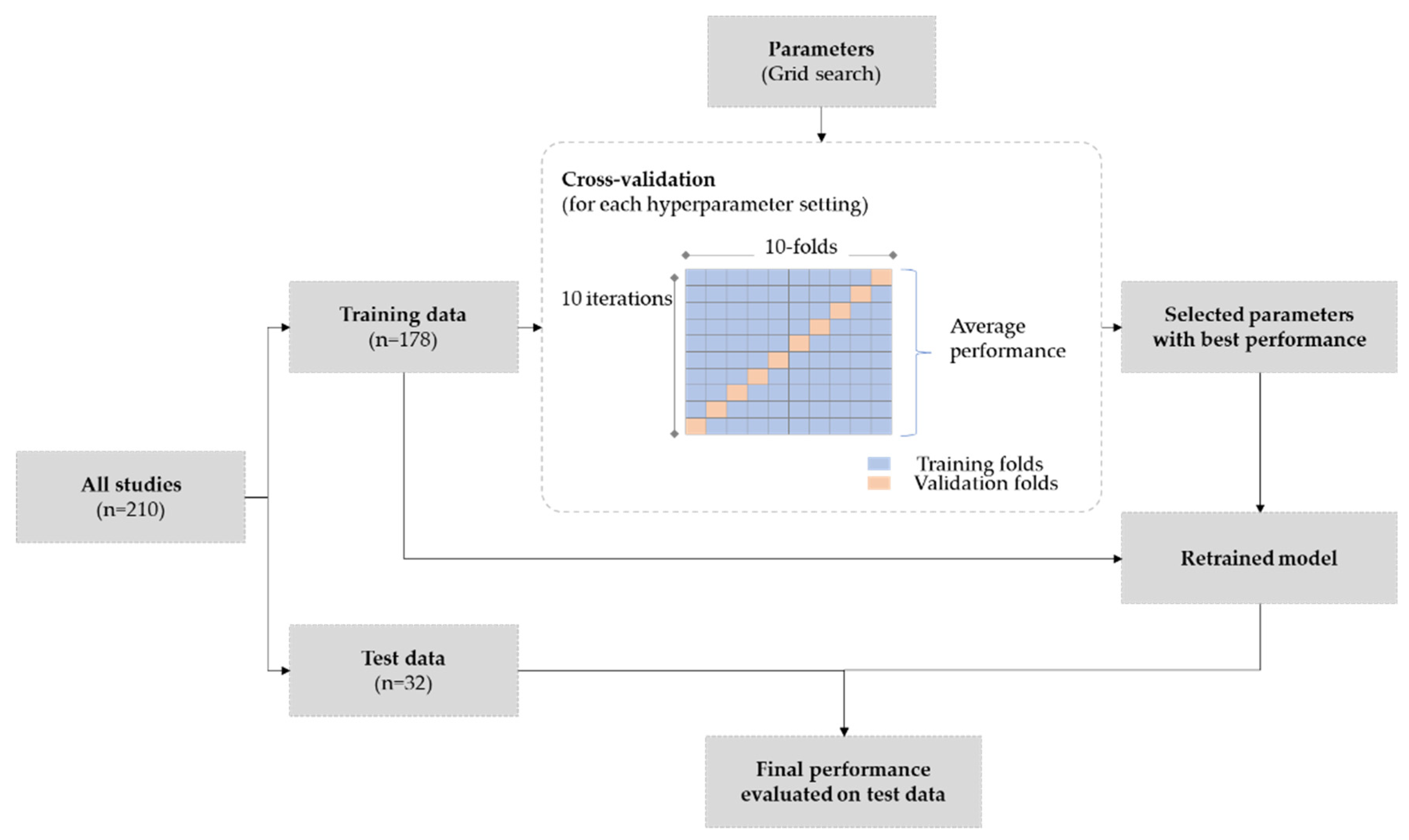
2.7. Training & Experiment Design
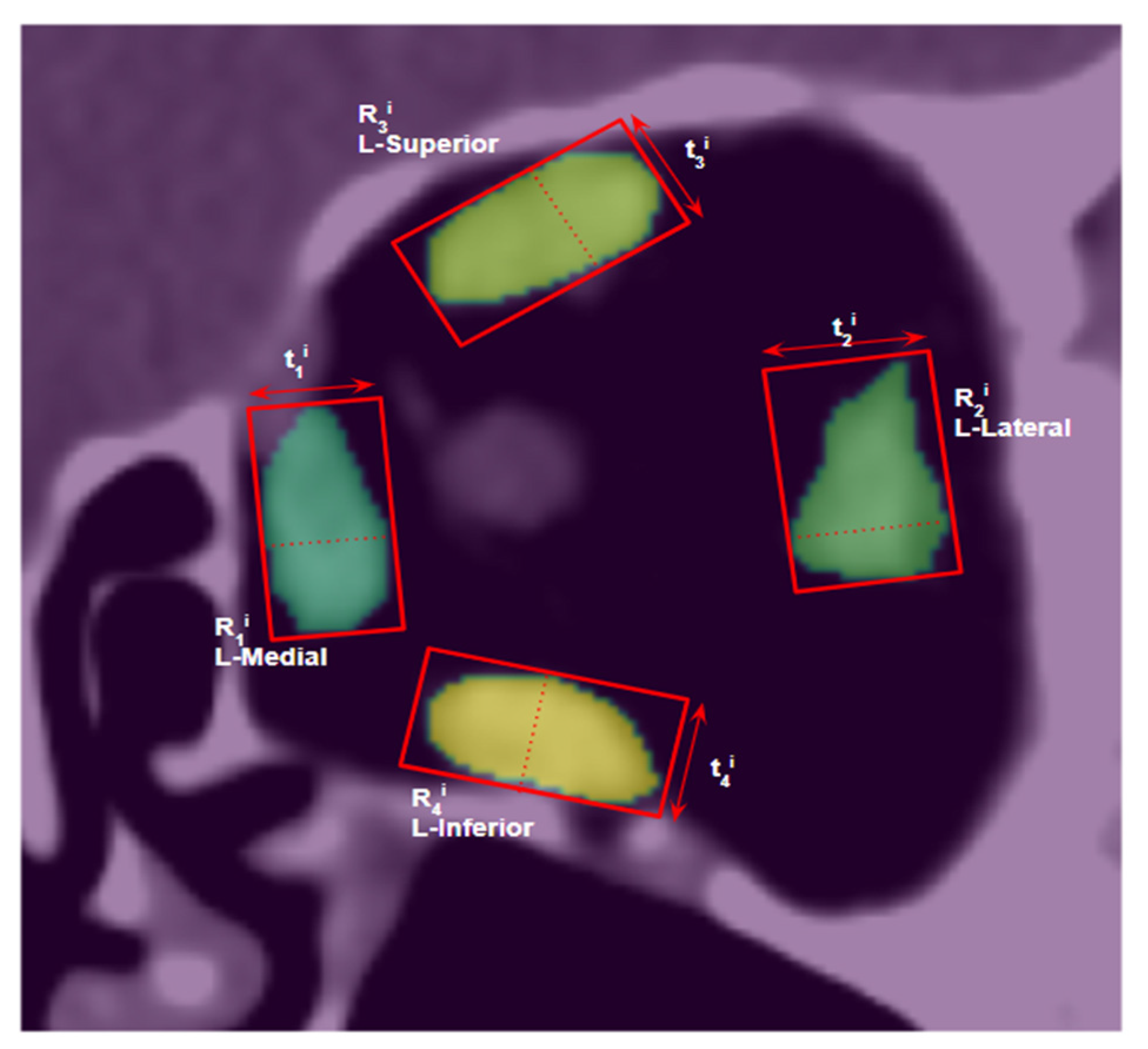
2.8. Muscle Size Measurement
2.9. Evaluation
3. Results
3.1. Quantitative Evaluation
3.1.1. Model Performance
3.1.2. Comparison of Muscle Size Measurements
3.1.3. Model Performance on Noisy Images
3.1.4. Performance Comparison with Traditional Segmentation Methods
3.2. Qualitative Evaluation
4. Discussion
5. Conclusions
Author Contributions
Funding
Institutional Review Board Statement
Informed Consent Statement
Data Availability Statement
Acknowledgments
Conflicts of Interest
References
- Szucs-Farkas, Z.; Toth, J.; Balazs, E.; Galuska, L.; Burman, K.D.; Karanyi, Z.; Leovey, A.; Nagy, E.V. Using morphologic parameters of extraocular muscles for diagnosis and follow-up of Graves’ ophthalmopathy: Diameters, areas, or volumes? AJR Am. J. Roentgenol. 2002, 179, 1005–1010. [Google Scholar] [CrossRef] [PubMed] [Green Version]
- Firbank, M.J.; Harrison, R.M.; Williams, E.D.; Coulthard, A. Measuring extraocular muscle volume using dynamic contours. Magn. Reson. Imaging 2001, 19, 257–265. [Google Scholar] [CrossRef]
- Lv, B.; Wu, T.; Lu, K.; Xie, Y. Automatic Segmentation of Extraocular Muscle Using Level Sets Methods with Shape Prior. IFMBE Proc. 2013, 39, 904–907. [Google Scholar] [CrossRef]
- Wei, Q.; Sueda, S.; Miller, J.M.; Demer, J.L.; Pai, D.K. Template-based reconstruction of human extraocular muscles from magnetic resonance images. In Proceedings of the 2009 IEEE International Symposium on Biomedical Imaging: From Nano to Macro, Boston, MA, USA, 28 June–1 July 2009; pp. 105–108. [Google Scholar] [CrossRef]
- Xing, Q.; Li, Y.; Wiggins, B.; Demer, J.; Wei, Q. Automatic Segmentation of Extraocular Muscles Using Superpixel and Normalized Cuts. Advances in Visual Computing; ISVC 2015. Lecture Notes in Computer Science; Springer: Cham, Switzerland, 2015; Volume 9474. [Google Scholar] [CrossRef]
- Ronneberger, O.; Fischer, P.; Brox, T. U-Net: Convolutional networks for biomedical image segmentation. In Medical Image Computing and Computer-Assisted Intervention (MICCAI); Navab, N., Hornegger, J., Wells, W.M., Frangi, A.F., Eds.; Springer: Cham, Switzerland, 2015; Volume 9351, pp. 234–241. [Google Scholar] [CrossRef] [Green Version]
- Milletari, F.; Navab, N.; Ahmadi, S. V-Net: Fully Convolutional Neural Networks for Volumetric Medical Image Segmentation. In Proceedings of the 2016 Fourth International Conference on 3D Vision (3DV), Stanford, CA, USA, 25–28 October 2016; pp. 565–571. [Google Scholar] [CrossRef] [Green Version]
- Jalali, Y.; Fateh, M.; Rezvani, M.; Abolghasemi, V.; Anisi, M.H. ResBCDU-Net: A Deep Learning Framework for Lung CT Image Segmentation. Sensors 2021, 21, 268. [Google Scholar] [CrossRef]
- Wang, T.; Xing, H.; Li, Y.; Wang, S.; Liu, L.; Li, F.; Jing, H. Deep learning-based automated segmentation of eight brain anatomical regions using head CT images in PET/CT. BMC Med. Imaging 2022, 22, 99. [Google Scholar] [CrossRef]
- Nikolov, S.; Blackwell, S.; Zverovitch, A.; Mendes, R.; Livne, M.; De Fauw, J.; Patel, Y.; Meyer, C.; Askham, H.; Romera-Paredes, B.; et al. Clinically Applicable Segmentation of Head and Neck Anatomy for Radiotherapy: Deep Learning Algorithm Development and Validation Study. J. Med. Internet Res. 2021, 23, e26151. [Google Scholar] [CrossRef]
- Kamnitsas, K.; Ledig, C.; Newcombe, V.F.; Simpson, J.P.; Kane, A.D.; Menon, D.K.; Rueckert, D.; Glocker, B. Efficient multi-scale 3D CNN with fully connected CRF for accurate brain lesion segmentation. Med. Image Anal. 2017, 36, 61–78. [Google Scholar] [CrossRef]
- Zhu, F.; Gao, Z.; Zhao, C.; Zhu, Z.; Tang, J.; Liu, Y.; Tang, S.; Jiang, C.; Li, X.; Zhao, M.; et al. Semantic segmentation using deep learning to extract total extraocular muscles and optic nerve from orbital computed tomography images. Optik 2021, 244, 167551. [Google Scholar] [CrossRef]
- Hanai, K.; Tabuchi, H.; Nagasato, D.; Tanabe, M.; Masumoto, H.; Nishio, S.; Nishio, N.; Nakamura, H.; Hashimoto, M. Automated Detection of Enlarged Extraocular Muscle In Graves’ Ophthalmopathy With Computed Tomography And Deep Neural Network. Res. Sq. 2022. [Google Scholar] [CrossRef]
- Ozgen, A.; Ariyurek, M. Normative Measurements of Orbital Structures Using CT. AJR Am. J. Roentgenol. 1998, 170, 1093–1096. [Google Scholar] [CrossRef]
- Xu, L.; Li, L.; Xie, C.; Guan, M.; Xue, Y. Thickness of Extraocular Muscle and Orbital Fat in MRI Predicts Response to Glucocorticoid Therapy in Graves’ Ophthalmopathy. Int. J. Endocrinol. 2017, 2017, 3196059. [Google Scholar] [CrossRef] [PubMed] [Green Version]
- Firbank, M.J.; Coulthard, A. Evaluation of a technique for estimation of extraocular muscle volume using 2D MRI. Br. J. Radiol. 2000, 73, 1282–1289. [Google Scholar] [CrossRef] [PubMed]
- Goodfellow, I.; Bengio, Y.; Courville, A. Deep Learning; MIT Press: Cambridge, MA, USA, 2016. [Google Scholar]
- Szeliski, R. Computer Vision: Algorithms and Applications; Springer Science & Business Media: Berlin/Heidelberg, Germany, 2010. [Google Scholar] [CrossRef]
- Geremia, E.; Menze, B.H.; Clatz, O.; Konukoglu, E.; Criminisi, A.; Ayache, N. Spatial decision forests for MS lesion segmentation in multi-channel MR images. In Medical Image Computing and Computer-Assisted Intervention—MICCAI; Springer: Berlin/Heidelberg, Germany, 2010; pp. 111–118. [Google Scholar] [CrossRef] [Green Version]
- Liu, X.; Song, L.; Liu, S.; Zhang, Y. A Review of Deep-Learning-Based Medical Image Segmentation Methods. Sustainability 2021, 13, 1224. [Google Scholar] [CrossRef]
- Long, J.; Shelhamer, E.; Darrell, T. Fully convolutional networks for semantic segmentation. In Proceedings of the IEEE Conference on Computer Vision and Pattern Recognition, Boston, MA, USA, 7–12 June 2015; pp. 3431–3440. [Google Scholar]
- Chen, L.; Papandreou, G.; Kokkinos, I.; Murphy, K.P.; Yuille, A.L. Semantic Image Segmentation with Deep Convolutional Nets and Fully Connected CRFs. arXiv 2015, arXiv:1412.7062. [Google Scholar]
- Chen, L.; Papandreou, G.; Kokkinos, I.; Murphy, K.; Yuille, A.L. DeepLab: Semantic Image Segmentation with Deep Convolutional Nets, Atrous Convolution, and Fully Connected CRFs. IEEE Trans. Pattern Anal. Mach. Intell. 2018, 40, 834–848. [Google Scholar] [CrossRef] [Green Version]
- Chen, L.; Papandreou, G.; Schroff, F.; Adam, H. Rethinking Atrous Convolution for Semantic Image Segmentation. arXiv 2017, arXiv:abs/1706.05587. [Google Scholar]
- Chen, L.C.; Zhu, Y.; Papandreou, G.; Schroff, F.; Adam, H. Encoder-decoder with atrous separable convolution for semantic image segmentation. In Proceedings of the European Conference on Computer Vision (ECCV), Munich, Germany, 8–14 September 2018; pp. 801–818. [Google Scholar]
- Krähenbühl, P.; Koltun, V. Efficient Inference in Fully Connected CRFs with Gaussian Edge Potentials. In Proceedings of the Advances in Neural Information Processing Systems, Granada, Spain, 12–15 December 2011. [Google Scholar]
- Badrinarayanan, V.; Kendall, A.; Cipolla, R. SegNet: A Deep Convolutional Encoder-Decoder Architecture for Image Segmentation. IEEE Trans. Pattern Anal. Mach. Intell. 2017, 39, 2481–2495. [Google Scholar] [CrossRef]
- Myronenko, A. 3D MRI brain tumor segmentation using autoencoder regularization. In Proceedings of the International MICCAI Brainlesion Workshop, Shenzhen, China, 17 October 2018; pp. 311–320. [Google Scholar]
- Nie, D.; Wang, L.; Adeli, E.; Lao, C.; Lin, W.; Shen, D. 3-D fully convolutional networks for multimodal isointense infant brain image segmentation. IEEE Trans. Cybern. 2019, 49, 1123–1136. [Google Scholar] [CrossRef]
- Wang, S.; Yi, L.; Chen, Q.; Meng, Z.; Dong, H.; He, Z. Edge-aware Fully Convolutional Network with CRF-RNN Layer for Hippocampus Segmentation. In Proceedings of the 2019 IEEE 8th Joint International Information Technology and Artificial Intelligence Conference (ITAIC), Chongqing, China, 24–26 May 2019; pp. 803–806. [Google Scholar]
- Edupuganti, V.G.; Chawla, A.; Amit, K. Automatic optic disk and cup segmentation of fundus images using deep learning. In Proceedings of the 25th IEEE International Conference on Image Processing (ICIP), Athens, Greece, 7–10 October 2018; pp. 2227–2231. [Google Scholar]
- Shankaranarayana, S.M.; Ram, K.; Mitra, K.; Sivaprakasam, M. Joint optic disc and cup segmentation using fully convolutional and adversarial networks. In Fetal, Infant and Ophthalmic Medical Image Analysis; Springer: Cham, Switzerland, 2017; pp. 168–176. [Google Scholar]
- Anthimopoulos, M.M.; Christodoulidis, S.; Ebner, L.; Geiser, T.; Christe, A.; Mougiakakou, S. Semantic Segmentation of Pathological Lung Tissue with Dilated Fully Convolutional Networks. IEEE J. Biomed. Health Inform. 2019, 23, 714–722. [Google Scholar] [CrossRef] [Green Version]
- Christ, P.F.; Ettlinger, F.; Grün, F.; Elshaera, M.E.A.; Lipkova, J.; Schlecht, S.; Ahmaddy, F.; Tatavarty, S.; Bickel, M.; Bilic, P.; et al. Automatic liver and tumor segmentation of CT and MRI volumes using cascaded fully convolutional neural networks. arXiv 2017, arXiv:1702.05970. [Google Scholar]
- Tran, P.V. A fully convolutional neural network for cardiac segmentation in short-axis MRI. arXiv 2016, arXiv:1604.00494. [Google Scholar]
- Çiçek, Ö.; Abdulkadir, A.; Lienkamp, S.S.; Brox, T.; Ronneberger, O. 3D U-Net: Learning dense volumetric segmentation from sparse annotation. In Proceedings of the International Conference on Medical Image Computing and Computer-Assisted Intervention, Athens, Greece, 17–21 October 2016; pp. 424–432. [Google Scholar]
- Oktay, O.; Schlemper, J.; Folgoc, L.L.; Lee, M.; Heinrich, M.; Misawa, K.; Mori, K.; Mcdonagh, S.; Hammerla, N.Y.; Kainz, B.; et al. Attention u-net: Learning where to look for the pancreas. arXiv 2018, arXiv:1804.03999. [Google Scholar]
- Zhang, Y.; Chung, A.C.S. Deep supervision with additional labels for retinal vessel segmentation task. In Proceedings of the International Conference on Medical Image Computing and Computer-Assisted Intervention, Granada, Spain, 16–20 September 2018; pp. 83–91. [Google Scholar]
- Novikov, A.A.; Lenis, D.; Major, D.; Uvka, J.H.; Wimmer, M.; Bühler, K. Fully convolutional architectures for multiclass segmentation in chest radiographs. IEEE Trans. Med. Imaging 2018, 37, 1865–1876. [Google Scholar] [CrossRef] [PubMed] [Green Version]
- Ye, C.; Wang, W.; Zhang, S.; Wang, K. Multi-depth fusion network for whole-heart CT image segmentation. IEEE Access 2019, 7, 23421–23429. [Google Scholar] [CrossRef]
- Luc, P.; Couprie, C.; Chintala, S.; Verbeek, J. Semantic segmentation using adversarial networks. arXiv 2016, arXiv:1611.08408. [Google Scholar]
- Moeskops, P.; Veta, M.; Lafarge, M.W.; Eppenhof, K.A.J.; Pluim, J.P.W. Adversarial training and dilated convolutions for brain MRI segmentation. In Deep Learning in Medical Image Analysis and Multimodal Learning for Clinical Decision Support; Springer: Cham, Switzerland, 2017; pp. 56–64. [Google Scholar]
- Son, J.; Park, S.J.; Jung, K.H. Retinal vessel segmentation in fundoscopic images with generative adversarial networks. arXiv 2017, arXiv:1706.09318. [Google Scholar]
- Han, Z.; Wei, B.; Mercado, A.; Leung, S.; Li, S. Spine-GAN: Semantic segmentation of multiple spinal structures. Med. Image Anal. 2018, 50, 23–35. [Google Scholar] [CrossRef]
- Fedorov, A.; Beichel, R.; Kalpathy-Cramer, J.; Finet, J.; Fillion-Robin, J.C.; Pujol, S.; Bauer, C.; Jennings, D.; Fennessy, F.; Sonka, M.; et al. 3D Slicer as an image computing platform for the Quantitative Imaging Network. Magn. Reson. Imaging 2012, 30, 1323–1341. [Google Scholar] [CrossRef] [Green Version]
- Frush, D.P.; Slack, C.C.; Hollingsworth, C.L.; Bisset, G.S.; Donnelly, L.F.; Hsieh, J.; Lavin-Wensell, T.; Mayo, J.R. Computer-simulated radiation dose reduction for abdominal multidetector CT of pediatric patients. AJR Am. J. Roentgenol. 2002, 179, 1107–1113. [Google Scholar] [CrossRef]
- Zeng, D.; Huang, J.; Bian, Z.; Niu, S.; Zhang, H.; Feng, Q.; Liang, Z.; Ma, J. A Simple Low-dose X-ray CT Simulation from High-dose Scan. IEEE Trans. Nucl. Sci. 2015, 62, 2226–2233. [Google Scholar] [CrossRef] [Green Version]
- Ma, J.; Chen, J.; Ng, M.; Huang, R.; Li, Y.; Li, C.; Yang, X.; Martel, A.L. Loss odyssey in medical image segmentation. Med. Image Anal. 2021, 71, 102035. [Google Scholar] [CrossRef] [PubMed]
- Dice, L.R. Measures of the Amount of Ecologic Association Between Species. Ecology 1945, 26, 297–302. [Google Scholar] [CrossRef]
- Rahman, M.A.; Wang, Y. Optimizing Intersection-Over-Union in Deep Neural Networks for Image Segmentation. Advances in Visual Computing; ISVC 2016. Lecture Notes in Computer Science; Springer: Cham, Switzerland, 2016; Volume 10072. [Google Scholar] [CrossRef]
- Abraham, N.; Khan, N.M. A Novel Focal Tversky Loss Function With Improved Attention U-Net for Lesion Segmentation. In Proceedings of the 2019 IEEE 16th International Symposium on Biomedical Imaging (ISBI 2019), Venice, Italy, 8–11 April 2019; pp. 683–687. [Google Scholar]
- Kervadec, H.; Bouchtiba, J.; Desrosiers, C.; Granger, E.; Dolz, J.; Ayed, I.B. Boundary loss for highly unbalanced segmentation. Med. Image Anal. 2021, 67, 101851. [Google Scholar] [CrossRef] [PubMed]
- Kingma, D.P.; Ba, J. Adam: A method for stochastic optimization. arXiv 2014, arXiv:1412.6980. [Google Scholar] [CrossRef]
- Srivastava, N.; Hinton, G.E.; Krizhevsky, A.; Sutskever, I.; Salakhutdinov, R. Dropout: A simple way to prevent neural networks from overfitting. J. Mach. Learn. Res. 2014, 15, 1929–1958. [Google Scholar]
- Glorot, X.; Bengio, Y. Understanding the difficulty of training deep feedforward neural networks. Proc. Thirteen. Int. Conf. Artif. Intell. Stat. Proc. Mach. Learn. Res. 2010, 9, 249–256. [Google Scholar]


| Train | Test | p-Value | |
|---|---|---|---|
| N | 178 | 32 | |
| Sex = M (%) | 53 (30%) | 9 (28%) | 1 |
| Age | 46.67 (17.49) | 50.97 (19.7) | 0.21 |
| Thickness—L-Medial Rectus | 4.87 (0.84) | 4.85 (0.7) | 0.9 |
| Thickness—L-Lateral Rectus | 5.5 (1.13) | 5.38 (1.18) | 0.58 |
| Thickness—L-Superior group | 4.79 (0.93) | 4.9 (0.77) | 0.53 |
| Thickness—L-Inferior Rectus | 5.23 (1.07) | 5.19 (1.02) | 0.84 |
| Thickness—R-Medial Rectus | 4.74 (0.66) | 4.66 (0.85) | 0.55 |
| Thickness—R-Lateral Rectus | 5.62 (1.41) | 5.87 (1.33) | 0.35 |
| Thickness—R-Superior group | 4.85 (1.04) | 4.99 (0.91) | 0.48 |
| Thickness—R-Inferior Rectus | 5.13 (1.08) | 4.97 (0.98) | 0.44 |
| Area—L-Medial Rectus | 38.93 (8.54) | 39.16 (6.55) | 0.89 |
| Area—L-Lateral Rectus | 46.03 (10.03) | 46.17 (12.05) | 0.89 |
| Area—L-Superior group | 38.29 (9.66) | 40.28 (8.04) | 0.27 |
| Area—L-Inferior Rectus | 41.57 (11.78) | 41.17 (9.35) | 0.86 |
| Area—R-Medial Rectus | 38.14 (6.88) | 38.56 (7.01) | 0.75 |
| Area—R-Lateral Rectus | 47.2 (14.29) | 49.81 (12.33) | 0.33 |
| Area—R-Superior group | 40.1 (13.79) | 41.39 (9.62) | 0.61 |
| Area—R-Inferior Rectus | 42.38 (14.24) | 41.14 (10.8) | 0.64 |
| Evaluation Metric | Muscle | Loss Function | ||||
|---|---|---|---|---|---|---|
| WCE | Dice | WCE + Dice | FTL | Dice + Boundary | ||
| Dice similarity coefficient (DSC) score | L-medial rectus | 0.90 ± 0.01 | 0.91 ± 0.03 | 0.93 ± 0.02 | 0.90 ± 0.05 | 0.94 ± 0.01 |
| L-lateral rectus | 0.90 ± 0.00 | 0.91 ± 0.04 | 0.91 ± 0.03 | 0.90 ± 0.05 | 0.93 ± 0.01 | |
| L-superior group | 0.84 ± 0.03 | 0.90 ± 0.03 | 0.91 ± 0.02 | 0.87 ± 0.06 | 0.87 ± 0.05 | |
| L-inferior rectus | 0.90 ± 0.02 | 0.92 ± 0.03 | 0.94 ± 0.02 | 0.90 ± 0.03 | 0.93 ± 0.02 | |
| R-Medial rectus | 0.90 ± 0.00 | 0.93 ± 0.02 | 0.94 ± 0.01 | 0.91 ± 0.02 | 0.93 ± 0.01 | |
| R-lateral rectus | 0.88 ± 0.01 | 0.91 ± 0.04 | 0.91 ± 0.04 | 0.88 ± 0.06 | 0.90 ± 0.05 | |
| R-superior group | 0.85 ± 0.01 | 0.89 ± 0.02 | 0.91 ± 0.02 | 0.87 ± 0.03 | 0.88 ± 0.03 | |
| R-inferior rectus | 0.91 ± 0.01 | 0.90 ± 0.04 | 0.92 ± 0.02 | 0.90 ± 0.05 | 0.92 ± 0.03 | |
| All | 0.89 ± 0.03 | 0.91 ± 0.03 | 0.92 ± 0.03 | 0.89 ± 0.05 | 0.91 ± 0.04 | |
| Jaccard (IOU) score | L-medial rectus | 0.81 ± 0.02 | 0.86 ± 0.04 | 0.88 ± 0.03 | 0.83 ± 0.07 | 0.89 ± 0.02 |
| L-lateral rectus | 0.83 ± 0.00 | 0.85 ± 0.05 | 0.86 ± 0.04 | 0.84 ± 0.06 | 0.87 ± 0.01 | |
| L-superior group | 0.73 ± 0.04 | 0.82 ± 0.04 | 0.85 ± 0.03 | 0.79 ± 0.07 | 0.80 ± 0.05 | |
| L-inferior rectus | 0.82 ± 0.03 | 0.86 ± 0.04 | 0.88 ± 0.03 | 0.83 ± 0.04 | 0.87 ± 0.04 | |
| R-medial rectus | 0.82 ± 0.00 | 0.87 ± 0.03 | 0.89 ± 0.01 | 0.84 ± 0.03 | 0.88 ± 0.02 | |
| R-lateral rectus | 0.79 ± 0.02 | 0.85 ± 0.05 | 0.85 ± 0.05 | 0.81 ± 0.07 | 0.84 ± 0.06 | |
| R-superior group | 0.75 ± 0.01 | 0.82 ± 0.02 | 0.84 ± 0.03 | 0.79 ± 0.03 | 0.80 ± 0.03 | |
| R-inferior rectus | 0.83 ± 0.02 | 0.84 ± 0.04 | 0.87 ± 0.03 | 0.83 ± 0.07 | 0.87 ± 0.04 | |
| All | 0.80 ± 0.04 | 0.85 ± 0.04 | 0.87 ± 0.04 | 0.82 ± 0.06 | 0.85 ± 0.05 | |
| Muscle | DSC Score | IOU Score |
|---|---|---|
| L-medial rectus | 0.94 ± 0.07 | 0.90 ± 0.09 |
| L-lateral rectus | 0.93 ± 0.09 | 0.88 ± 0.10 |
| L-superior group | 0.90 ± 0.12 | 0.83 ± 0.13 |
| L-inferior rectus | 0.94 ± 0.08 | 0.90 ± 0.08 |
| R-medial rectus | 0.92 ± 0.16 | 0.88 ± 0.17 |
| R-lateral rectus | 0.93 ± 0.04 | 0.88 ± 0.06 |
| R-superior group | 0.87 ± 0.14 | 0.80 ± 0.15 |
| R-inferior rectus | 0.93 ± 0.09 | 0.88 ± 0.11 |
| All | 0.92 ± 0.02 | 0.87 ± 0.03 |
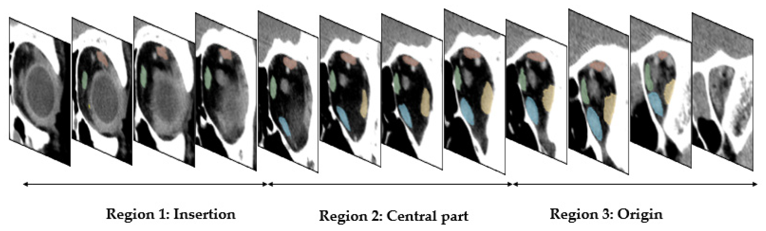
| Muscle | Region 1: Insertion | Region 2: Central Part | Region 3: Origin | |||
|---|---|---|---|---|---|---|
| L-medial rectus | 0.89 ± 0.13 | 0.82 ± 0.16 | 0.97 ± 0.01 | 0.94 ± 0.02 | 0.91 ± 0.10 | 0.85 ± 0.13 |
| L-lateral rectus | 0.88 ± 0.15 | 0.81 ± 0.15 | 0.95 ± 0.02 | 0.90 ± 0.03 | 0.94 ± 0.08 | 0.89 ± 0.09 |
| L-superior group | 0.79 ± 0.26 | 0.71 ± 0.25 | 0.92 ± 0.06 | 0.86 ± 0.07 | 0.92 ± 0.05 | 0.85 ± 0.08 |
| L-inferior rectus | 0.93 ± 0.04 | 0.88 ± 0.06 | 0.94 ± 0.07 | 0.89 ± 0.08 | 0.95 ± 0.02 | 0.90 ± 0.04 |
| R-medial rectus | 0.91 ± 0.16 | 0.85 ± 0.16 | 0.79 ± 0.34 | 0.75 ± 0.35 | 0.83 ± 0.25 | 0.77 ± 0.25 |
| R-lateral rectus | 0.77 ± 0.20 | 0.66 ± 0.21 | 0.93 ± 0.03 | 0.87 ± 0.05 | 0.94 ± 0.04 | 0.89 ± 0.06 |
| R-superior group | 0.78 ± 0.29 | 0.70 ± 0.28 | 0.91 ± 0.04 | 0.84 ± 0.06 | 0.89 ± 0.04 | 0.80 ± 0.07 |
| R-inferior rectus | 0.89 ± 0.16 | 0.83 ± 0.16 | 0.95 ± 0.07 | 0.90 ± 0.08 | 0.94 ± 0.03 | 0.88 ± 0.06 |
| All | 0.86 ± 0.20 | 0.78 ± 0.20 | 0.92 ± 0.14 | 0.87 ± 0.15 | 0.91 ± 0.11 | 0.86 ± 0.12 |
| Muscle | MAE Thickness (mm) | MAPE Thickness | MAE Area (mm2) | MAPE Area |
|---|---|---|---|---|
| L-medial rectus | 0.24 | 5% | 1.99 | 6% |
| L-lateral rectus | 0.35 | 7% | 6.53 | 14% |
| L-superior group | 0.37 | 8% | 3.15 | 8% |
| L-inferior rectus | 0.26 | 6% | 4.2 | 10% |
| R-medial rectus | 0.41 | 7% | 3.93 | 8% |
| R-lateral rectus | 0.46 | 9% | 3.85 | 10% |
| R-superior group | 0.33 | 7% | 4.09 | 10% |
| R-inferior rectus | 0.36 | 8% | 3.18 | 9% |
| All | 0.35 | 7% | 3.87 | 9% |
| Without Added Noise | With Added Noise (μ = 0, σ = 5) | With Added Noise (μ = 0, σ = 10) | |
|---|---|---|---|
| L-medial rectus | 0.94 ± 0.07 | 0.94 ± 0.08 | 0.93 ± 0.09 |
| L-lateral rectus | 0.93 ± 0.09 | 0.93 ± 0.07 | 0.92 ± 0.09 |
| L-superior group | 0.90 ± 0.12 | 0.89 ± 0.15 | 0.90 ± 0.13 |
| L-inferior rectus | 0.94 ± 0.08 | 0.94 ± 0.04 | 0.94 ± 0.09 |
| R-medial rectus | 0.92 ± 0.16 | 0.93 ± 0.10 | 0.92 ± 0.14 |
| R-lateral rectus | 0.93 ± 0.04 | 0.92 ± 0.08 | 0.92 ± 0.07 |
| R-superior group | 0.87 ± 0.14 | 0.86 ± 0.16 | 0.86 ± 0.17 |
| R-inferior rectus | 0.93 ± 0.09 | 0.93 ± 0.08 | 0.93 ± 0.07 |
| All | 0.92 ± 0.02 | 0.92 ± 0.12 | 0.92 ± 0.12 |
| Muscle | SU-Net | SV-Net | 2D Coronal U-Net |
|---|---|---|---|
| Medial rectus | 0.82 ± 2.83×10⁻⁵ | 0.84 ± 3.62 × 10⁻⁵ | 0.91 ± 0.12 |
| Lateral rectus | 0.80 ± 5.83 × 10⁻⁵ | 0.82 ± 3.56 × 10⁻⁵ | 0.89 ± 0.04 |
| Superior rectus | 0.73 ± 9.73 × 10⁻⁵ | 0.74 ± 7.84 × 10⁻⁵ | - |
| Superior muscle group | - | - | 0.84 ± 0.09 |
| Inferior rectus | 0.82 ± 2.83 × 10⁻⁵ | 0.84 ± 3.39 × 10⁻⁵ | 0.89 ± 0.06 |
| Optic nerve | 0.81 ± 1.77 × 10⁻⁴ | 0.82 ± 9.96 × 10⁻⁵ | - |
| Total | 0.80 ± 2.56 × 10⁻⁵ | 0.82 ± 3.22 × 10⁻⁵ | 0.88 ± 0.09 |
Publisher’s Note: MDPI stays neutral with regard to jurisdictional claims in published maps and institutional affiliations. |
© 2022 by the authors. Licensee MDPI, Basel, Switzerland. This article is an open access article distributed under the terms and conditions of the Creative Commons Attribution (CC BY) license (https://creativecommons.org/licenses/by/4.0/).
Share and Cite
Shanker, R.R.B.J.; Zhang, M.H.; Ginat, D.T. Semantic Segmentation of Extraocular Muscles on Computed Tomography Images Using Convolutional Neural Networks. Diagnostics 2022, 12, 1553. https://doi.org/10.3390/diagnostics12071553
Shanker RRBJ, Zhang MH, Ginat DT. Semantic Segmentation of Extraocular Muscles on Computed Tomography Images Using Convolutional Neural Networks. Diagnostics. 2022; 12(7):1553. https://doi.org/10.3390/diagnostics12071553
Chicago/Turabian StyleShanker, Ramkumar Rajabathar Babu Jai, Michael H. Zhang, and Daniel T. Ginat. 2022. "Semantic Segmentation of Extraocular Muscles on Computed Tomography Images Using Convolutional Neural Networks" Diagnostics 12, no. 7: 1553. https://doi.org/10.3390/diagnostics12071553
APA StyleShanker, R. R. B. J., Zhang, M. H., & Ginat, D. T. (2022). Semantic Segmentation of Extraocular Muscles on Computed Tomography Images Using Convolutional Neural Networks. Diagnostics, 12(7), 1553. https://doi.org/10.3390/diagnostics12071553