


Quantitative Assessment of Breast-Tumor Stiffness Using Shear-Wave Elastography Histograms

 ,
,  , and
, and 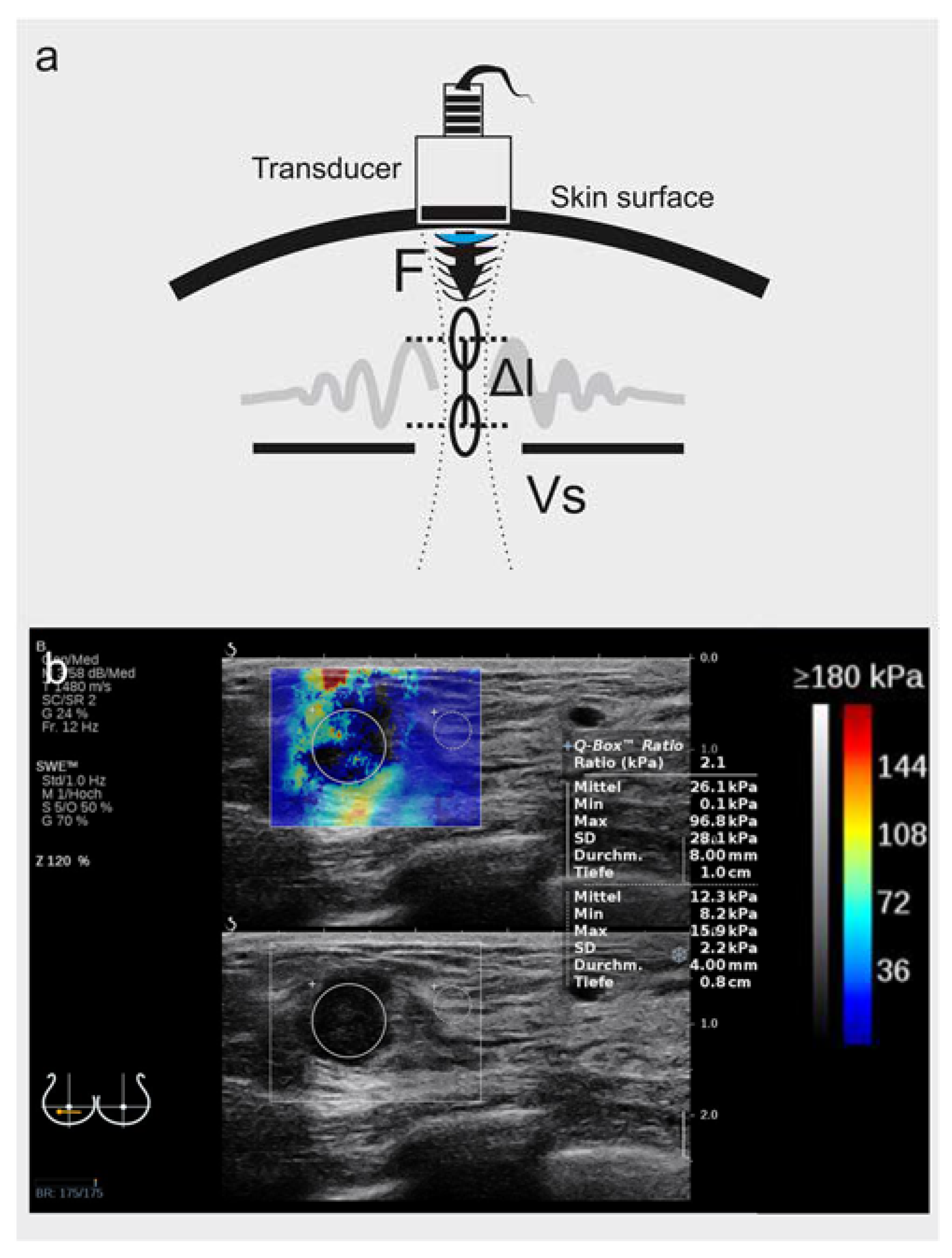
Abstract
1. Introduction
2. Materials and Methods
2.1. Patient Selection Criteria and Ground Truth
2.2. B-Mode and Shear-Wave Elastography Imaging
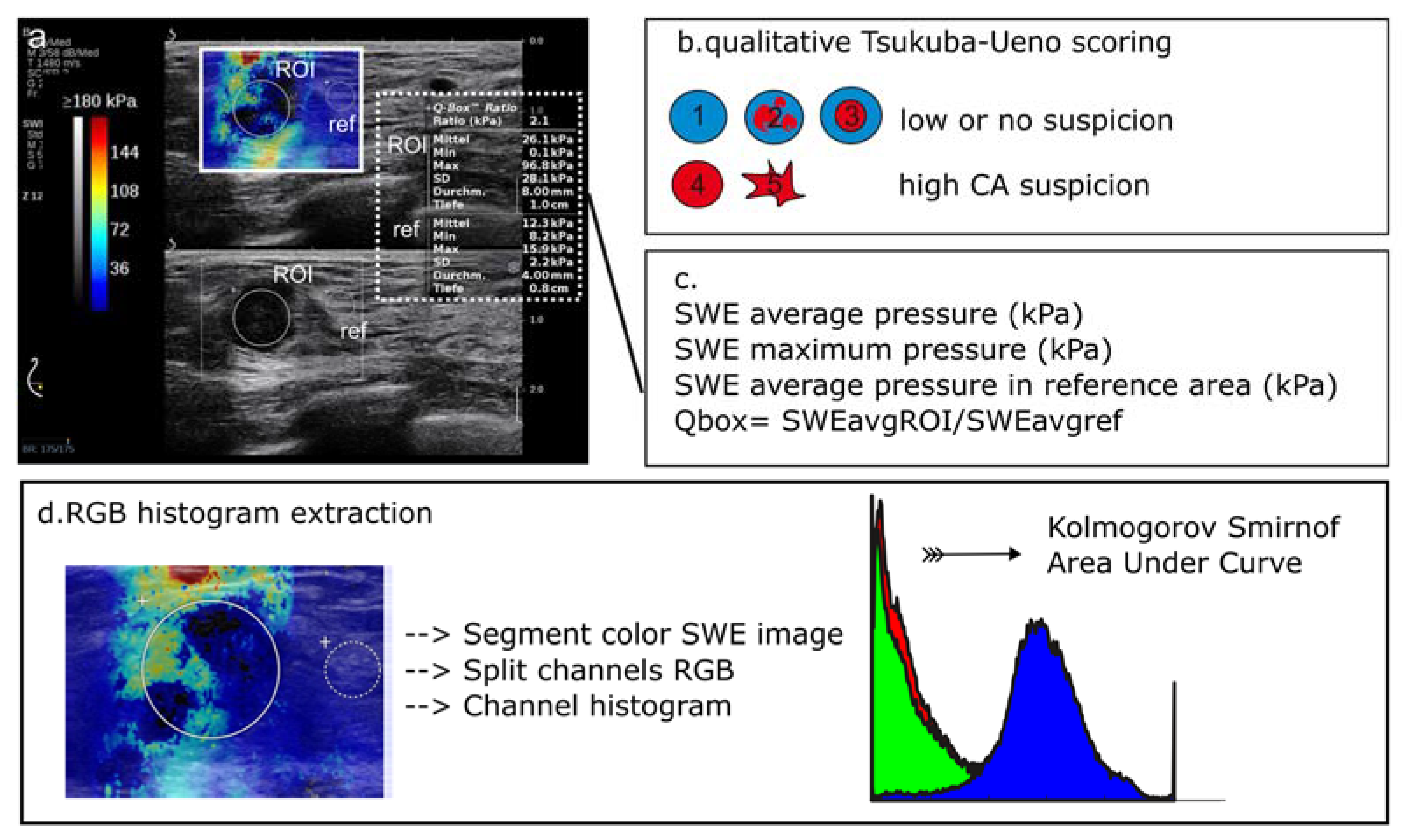
2.3. Image Analysis for Shear-Wave Elastography
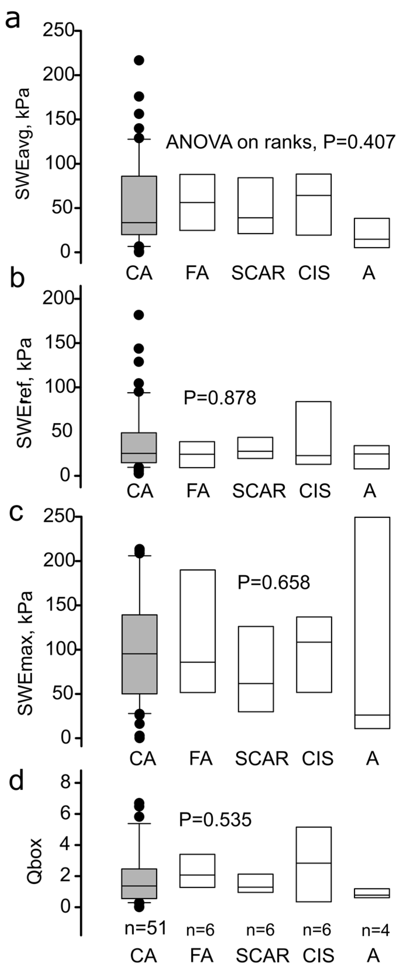
2.3.1. Local Average SWE Metrics
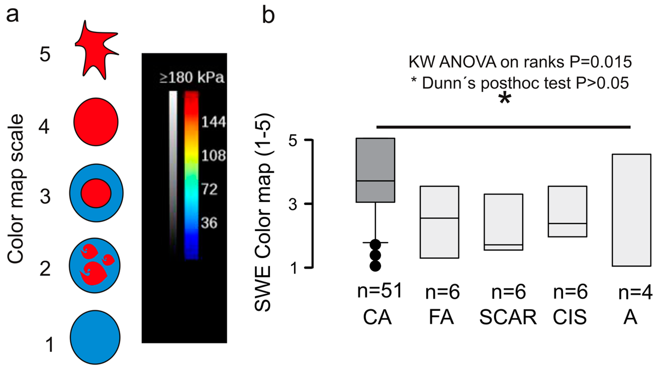
2.3.2. RGB Histogram
2.4. Statistics and Software
3. Result
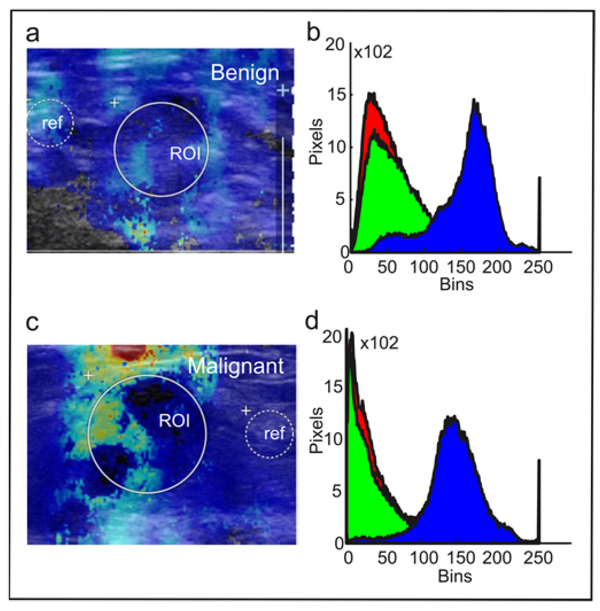
3.1. RGB Histograms Discriminate Malignant from Benign Tumors
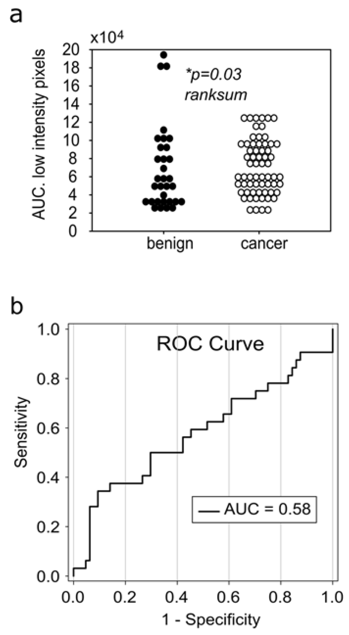
3.2. The Reduction of Soft-Tissue Components Is a Potential Biomarker for Breast Malignancy
3.3. Receiver Operating Curves for RGB Histograms
4. Discussion
4.1. Discriminative Value of the Local SWE Average, State of the Art
4.2. The Role of Anisotropy in Tumor Classification
4.3. Histogram SWE Analysis, Experience from Previous Studies, and the Role of Deep Learning
4.4. Effect of the ROI Size and Surrounding Tissue in SWE Interpretation
4.5. Study Weaknesses
5. Conclusions and Clinical Significance
Supplementary Materials
Author Contributions
Funding
Institutional Review Board Statement
Informed Consent Statement
Data Availability Statement
Conflicts of Interest
Abbreviations
| AI | Artificial intelligence |
| ANOVA | Analysis of variance |
| AUC | Area under curve |
| CA | Cancer |
| CIS | Cancer in situ |
| FA | Fibroadenoma |
| RGB | Red-green-blue |
| ROC | Receiver operating curve |
| ROI | Region of interest |
| SD | Standard deviation |
| SE | Strain elastography |
| Se | Sensitivity |
| Spe | Specificity |
| SWE | Shear-wave elastography |
| SWEavg | Average stiffness in kPa |
| SWEmax | Maximum stiffness in kPa |
| SWEref | Average stiffness of the reference region in kPa |
References
- Baker, E.L.; Lu, J.; Yu, D.; Bonnecaze, R.T.; Zaman, M.H. Zaman, Cancer Cell Stiffness: Integrated Roles of Three-Dimensional Matrix Stiffness and Transforming Potential. Biophys. J. 2010, 99, 2048–2057. [Google Scholar] [CrossRef] [PubMed]
- Gkretsi, V.; Stylianopoulos, T. Cell Adhesion and Matrix Stiffness: Coordinating Cancer Cell Invasion and Metastasis. Front. Oncol. 2018, 8, 145. [Google Scholar] [CrossRef] [PubMed]
- Dietrich, C.F.; Barr, R.G.; Farrokh, A.; Dighe, M.; Hocke, M.; Jenssen, C.; Dong, Y.; Saftoiu, A.; Havre, R.F. Strain Elastography—How to Do It? Ultrasound Int. Open. 2017, 3, E137–E149. [Google Scholar] [CrossRef] [PubMed]
- Sigrist, R.M.S.; Liau, J.; Kaffas, A.E.; Chammas, M.C.; Willmann, J.K. Ultrasound Elastography: Review of Techniques and Clinical Applications. Theranostics 2017, 7, 1303–1329. [Google Scholar] [CrossRef]
- Gennisson, J.-L.; Deffieux, T.; Fink, M.; Tanter, M. Ultrasound elastography: Principles and techniques. Diagn. Interv. Imaging. 2013, 94, 487–495. [Google Scholar] [CrossRef]
- Jeong, W.K.; Lim, H.K.; Lee, H.-K.; Jo, J.M.; Kim, Y. Principles and clinical application of ultrasound elastography for diffuse liver disease. Ultrasonography (Seoul Korea) 2014, 33, 149–160. [Google Scholar] [CrossRef]
- Nitta, N.; Yamakawa, M.; Hachiya, H.; Shiina, T. A review of physical and engineering factors potentially affecting shear wave elastography. J. Med. Ultrason. 2021, 48, 403–414. [Google Scholar] [CrossRef]
- Prado-Costa, R.; Rebelo, J.; Monteiro-Barroso, J.; Preto, A.S. Ultrasound elastography: Compression elastography and shear-wave elastography in the assessment of tendon injury. Insights Into Imaging 2018, 9, 791–814. [Google Scholar] [CrossRef]
- Barr, R.G.; Nakashima, K.; Amy, D.; Cosgrove, D.; Farrokh, A.; Schafer, F.; Bamber, J.C.; Castera, L.; Choi, B.I.; Chou, Y.-H.; et al. WFUMB guidelines and recommendations for clinical use of ultrasound elastography: Part 2: Breast. Ultrasound Med. Biol. 2015, 41, 1148–1160. [Google Scholar] [CrossRef]
- Ferraioli, G. Review of Liver Elastography Guidelines. J. Ultrasound Med. 2019, 38, 9–14. [Google Scholar] [CrossRef]
- Kim, J.R.; Suh, C.H.; Yoon, H.M.; Lee, J.S.; Cho, Y.A.; Jung, A.Y. The diagnostic performance of shear-wave elastography for liver fibrosis in children and adolescents: A systematic review and diagnostic meta-analysis. Eur. Radiol. 2018, 28, 1175–1186. [Google Scholar] [CrossRef] [PubMed]
- Pruijssen, J.T.; de Korte, C.L.; Voss, I.; Hansen, H.H.G. Vascular Shear Wave Elastography in Atherosclerotic Arteries: A Systematic Review. Ultrasound Med. Biol. 2020, 46, 2145–2163. [Google Scholar] [CrossRef] [PubMed]
- Grażyńska, A.; Kufel, J.; Dudek, A.; Cebula, M. Shear Wave and Strain Elastography in Crohn’s Disease—A Systematic Review. Diagn. Basel Switz. 2021, 11, 1609. [Google Scholar] [CrossRef] [PubMed]
- Swan, K.Z.; Nielsen, V.E.; Bonnema, S.J. Evaluation of thyroid nodules by shear wave elastography: A review of current knowledge. J. Endocrinol. Investig. 2021, 44, 2043–2056. [Google Scholar] [CrossRef] [PubMed]
- Moraes, P.H.M.; Takahashi, M.S.; Vanderlei, F.A.B.; Schelini, M.V.; Chacon, D.A.; Tavares, M.R.; Chammas, M.C. Multiparametric Ultrasound Evaluation of the Thyroid: Elastography as a Key Tool in the Risk Prediction of Undetermined Nodules (Bethesda III and IV)—Histopathological Correlation. Ultrasound Med. Biol. 2021, 47, 1219–1226. [Google Scholar] [CrossRef]
- Anbarasan, T.; Wei, C.; Bamber, J.C.; Barr, R.G.; Nabi, G. Characterisation of Prostate Lesions Using Transrectal Shear Wave Elastography (SWE) Ultrasound Imaging: A Systematic Review. Cancers 2021, 13, 122. [Google Scholar] [CrossRef]
- Bian, J.; Zhang, J.; Hou, X. Diagnostic accuracy of ultrasound shear wave elastography combined with superb microvascular imaging for breast tumors: A protocol for systematic review and meta-analysis. Medicine (Baltimore) 2021, 100, e26262. [Google Scholar] [CrossRef]
- Carlsen, J.; Ewertsen, C.; Sletting, S.; Vejborg, I.; Schäfer, F.K.W.; Cosgrove, D.; Nielsen, M.B. Ultrasound Elastography in Breast Cancer Diagnosis. Ultraschall Med. Stuttg. Ger. 2015, 36, 550–565. [Google Scholar] [CrossRef]
- Chang, J.M.; Won, J.-K.; Lee, K.-B.; Park, I.A.; Yi, A.; Moon, W.K. Comparison of shear-wave and strain ultrasound elastography in the differentiation of benign and malignant breast lesions. AJR Am. J. Roentgenol. 2013, 201, W347–W356. [Google Scholar] [CrossRef]
- Itoh, A.; Ueno, E.; Tohno, E.; Kamma, H.; Takahashi, H.; Shiina, T.; Yamakawa, M.; Matsumura, T. Breast disease: Clinical application of US elastography for diagnosis. Radiology 2006, 239, 341–350. [Google Scholar] [CrossRef]
- Xu, Y.-J.; Gong, H.-L.; Hu, B.; Hu, B. Role of “Stiff Rim” sign obtained by shear wave elastography in diagnosis and guiding therapy of breast cancer. Int. J. Med. Sci. 2021, 18, 3615–3623. [Google Scholar] [CrossRef] [PubMed]
- Zhou, J.; Zhan, W.; Chang, C.; Zhang, X.; Jia, Y.; Dong, Y.; Zhou, C.; Sun, J.; Grant, E.G. Breast lesions: Evaluation with shear wave elastography, with special emphasis on the “stiff rim” sign. Radiology 2014, 272, 63–72. [Google Scholar] [CrossRef] [PubMed]
- Cong, R.; Li, J.; Guo, S. A new qualitative pattern classification of shear wave elastograghy for solid breast mass evaluation. Eur. J. Radiol. 2017, 87, 111–119. [Google Scholar] [CrossRef]
- Gweon, H.M.; Youk, J.H.; Son, E.J.; Kim, J.-A. Visually assessed colour overlay features in shear-wave elastography for breast masses: Quantification and diagnostic performance. Eur. Radiol. 2013, 23, 658–663. [Google Scholar] [CrossRef] [PubMed]
- Park, J.; Woo, O.H.; Shin, H.S.; Cho, K.R.; Seo, B.K.; Kang, E.Y. Diagnostic performance and color overlay pattern in shear wave elastography (SWE) for palpable breast mass. Eur. J. Radiol. 2015, 84, 1943–1948. [Google Scholar] [CrossRef]
- Chen, Y.-L.; Gao, Y.; Chang, C.; Wang, F.; Zeng, W.; Chen, J.-J. Ultrasound shear wave elastography of breast lesions: Correlation of anisotropy with clinical and histopathological findings. Cancer Imaging Off. Publ. Int. Cancer Imaging Soc. 2018, 18, 11. [Google Scholar] [CrossRef]
- Zhang, Q.; Xiao, Y.; Chen, S.; Wang, C.; Zheng, H. Quantification of elastic heterogeneity using contourlet-based texture analysis in shear-wave elastography for breast tumor classification. Ultrasound Med. Biol. 2015, 41, 588–600. [Google Scholar] [CrossRef]
- Bove, S.; Comes, M.C.; Lorusso, V.; Cristofaro, C.; Didonna, V.; Gatta, G.; Giotta, F.; la Forgia, D.; Latorre, A.; Pastena, M.I.; et al. A ultrasound-based radiomic approach to predict the nodal status in clinically negative breast cancer patients. Sci. Rep. 2022, 12, 7914. [Google Scholar] [CrossRef]
- Au, F.W.F.; Ghai, S.; Moshonov, H.; Kahn, H.; Brennan, C.; Dua, H.; Crystal, P. Crystal, Diagnostic performance of quantitative shear wave elastography in the evaluation of solid breast masses: Determination of the most discriminatory parameter. AJR Am. J. Roentgenol. 2014, 203, W328–W336. [Google Scholar] [CrossRef]
- Yoon, J.H.; Ko, K.H.; Jung, H.K.; Lee, J.T. Qualitative pattern classification of shear wave elastography for breast masses: How it correlates to quantitative measurements. Eur. J. Radiol. 2013, 82, 2199–2204. [Google Scholar] [CrossRef]
- Yu, Y.; Xiao, Y.; Cheng, J.; Chiu, B. Breast lesion classification based on supersonic shear-wave elastography and automated lesion segmentation from B-mode ultrasound images. Comput. Biol. Med. 2018, 93, 31–46. [Google Scholar] [CrossRef] [PubMed]
- Pillai, A.; Voruganti, T.; Barr, R.; Langdon, J. Diagnostic Accuracy of Shear-Wave Elastography for Breast Lesion Characterization in Women: A Systematic Review and Meta-Analysis. J. Am. Coll. Radiol. 2022, 19, 625–634.e0. [Google Scholar] [CrossRef] [PubMed]
- Blank, M.A.B.; Antaki, J.F. Breast Lesion Elastography Region of Interest Selection and Quantitative Heterogeneity: A Systematic Review and Meta-Analysis. Ultrasound Med. Biol. 2017, 43, 387–397. [Google Scholar] [CrossRef]
- Carlsen, J.F.; Ewertsen, C.; Sletting, S.; Talman, M.L.; Vejborg, I.; Bachmann Nielsen, M. Bachmann Nielsen, Strain histograms are equal to strain ratios in predicting malignancy in breast tumours. PLoS ONE 2017, 12, e0186230. [Google Scholar] [CrossRef]
- Xue, S.-S.; Zhao, Q.-L.; Ruan, L.-T.; Wang, F.-Q.; Zhou, C.; Sheng, W. Comparative analysis of the quantitative parameter method and elasticity color mode method for real-time shear wave elastography in the diagnosis of benign and malignant solid breast lesions. Tumori J. 2022, 108, 578–585. [Google Scholar] [CrossRef] [PubMed]
- Cheng, M.-Q.; Xian, M.-F.; Tian, W.-S.; Li, M.-D.; Hu, H.-T.; Li, W.; Zhang, J.-C.; Huang, Y.; Xie, X.-Y.; Lu, M.-D.; et al. RGB Three-Channel SWE-Based Ultrasomics Model: Improving the Efficiency in Differentiating Focal Liver Lesions. Front. Oncol. 2021, 11, 3772. [Google Scholar] [CrossRef] [PubMed]
- Zhang, X.; Liang, M.; Yang, Z.; Zheng, C.; Wu, J.; Ou, B.; Li, H.; Wu, X.; Luo, B.; Shen, J. Deep Learning-Based Radiomics of B-Mode Ultrasonography and Shear-Wave Elastography: Improved Performance in Breast Mass Classification. Front. Oncol. 2020, 10, 1621. [Google Scholar] [CrossRef]
- Zhou, Y.; Xu, J.; Liu, Q.; Li, C.; Liu, Z.; Wang, M.; Zheng, H.; Wang, S. A Radiomics Approach With CNN for Shear-Wave Elastography Breast Tumor Classification. IEEE Trans. Biomed. Eng. 2018, 65, 1935–1942. [Google Scholar] [CrossRef]
- Jiang, M.; Li, C.-L.; Chen, R.-X.; Tang, S.-C.; Lv, W.-Z.; Luo, X.-M.; Chuan, Z.-R.; Jin, C.-Y.; Liao, J.-T.; Cui, X.-W.; et al. Management of breast lesions seen on US images: Dual-model radiomics including shear-wave elastography may match performance of expert radiologists. Eur. J. Radiol. 2021, 141, 109781. [Google Scholar] [CrossRef]
- van der Velden, B.H.M.; Kuijf, H.J.; Gilhuijs, K.G.A.; Viergever, M.A. Explainable artificial intelligence (XAI) in deep learning-based medical image analysis. Med. Image Anal. 2022, 79, 102470. [Google Scholar] [CrossRef]
- Moon, J.H.; Hwang, J.-Y.; Park, J.S.; Koh, S.H.; Park, S.-Y. Impact of region of interest (ROI) size on the diagnostic performance of shear wave elastography in differentiating solid breast lesions. Acta Radiol. Stockh. Swed. 2018, 59, 657–663. [Google Scholar] [CrossRef] [PubMed]
- Huang, Y.-S.; Takada, E.; Konno, S.; Huang, C.-S.; Kuo, M.-H.; Chang, R.-F. Computer-Aided tumor diagnosis in 3-D breast elastography. Comput. Methods Programs Biomed. 2018, 153, 201–209. [Google Scholar] [CrossRef] [PubMed]
- Lee, S.; Jung, Y.; Bae, Y. Clinical application of a color map pattern on shear-wave elastography for invasive breast cancer. Surg. Oncol. 2016, 25, 44–48. [Google Scholar] [CrossRef] [PubMed]


Publisher’s Note: MDPI stays neutral with regard to jurisdictional claims in published maps and institutional affiliations. |
© 2022 by the authors. Licensee MDPI, Basel, Switzerland. This article is an open access article distributed under the terms and conditions of the Creative Commons Attribution (CC BY) license (https://creativecommons.org/licenses/by/4.0/).
Share and Cite
Papageorgiou, I.; Valous, N.A.; Hadjidemetriou, S.; Teichgräber, U.; Malich, A. Quantitative Assessment of Breast-Tumor Stiffness Using Shear-Wave Elastography Histograms. Diagnostics 2022, 12, 3140. https://doi.org/10.3390/diagnostics12123140
Papageorgiou I, Valous NA, Hadjidemetriou S, Teichgräber U, Malich A. Quantitative Assessment of Breast-Tumor Stiffness Using Shear-Wave Elastography Histograms. Diagnostics. 2022; 12(12):3140. https://doi.org/10.3390/diagnostics12123140
Chicago/Turabian StylePapageorgiou, Ismini, Nektarios A. Valous, Stathis Hadjidemetriou, Ulf Teichgräber, and Ansgar Malich. 2022. "Quantitative Assessment of Breast-Tumor Stiffness Using Shear-Wave Elastography Histograms" Diagnostics 12, no. 12: 3140. https://doi.org/10.3390/diagnostics12123140
APA StylePapageorgiou, I., Valous, N. A., Hadjidemetriou, S., Teichgräber, U., & Malich, A. (2022). Quantitative Assessment of Breast-Tumor Stiffness Using Shear-Wave Elastography Histograms. Diagnostics, 12(12), 3140. https://doi.org/10.3390/diagnostics12123140