2. C and N Isotope Ratios in the Modern Earth Atmosphere
As an example of how isotope ratios vary among molecules in the present-day atmosphere, I will first consider carbon in CO
2 and CH
4. Ignoring anthropogenic input, the CO
2 mixing ratio is determined by the balance of CO
2 emitted by volcanism and the sequestration of CO
2 in marine carbonates, primarily by biological organisms. Rather than compute CO
2 I will focus on the geochemcial processes that alter its isotope composition. The δ
13C ratio of CO
2 is determined primarily by CO
2 exchange with the oceans. The massive reservoir of HCO
3− in the oceans and the high exchange flux between the atmosphere and oceanic mixed layer fix the C isotope ratios in the ocean. Neglecting CO
2 photolysis in the upper atmosphere, a process that is not important for tropospheric isotope ratios, δ
13C for CO
2 is −8.4 permil today and was about −6.5 permil in the pre-industrial atmosphere [
18]. The pre-industrial δ
13C value for CO
2 is close to the mantle value of −5 to −8‰ [
19]. Photosynthesis, respiration, and air-sea exchange all contribute to the fractionation of C isotopes. Fractionation during photosynthesis creates fixed C with δ
13C values 18 and 4‰ lower than those of atmospheric CO
2 for C
3 and C
4 plants, respectively [
20]. The predominance of C
3 plants (about 85%) yields a terrestrial bulk biosphere with δ
13C ~−22% relative to VPDB.
Expressing the δ
13C of atmospheric CO
2 in terms of its sources, we have
where
φ is the CO
2 flux due to either plant respiration or emissions associated with air-ocean exchange. The fluxes of C are
φplant resp = 60 Gt C yr
−1 and
φocean exch = 90 Gt C yr
−1, and the representative δ-values are −22‰ for plants and +2.5‰ for surface dissolved inorganic carbon (DIC). Air-sea exchange results in kinetic and equilibrium isotope enrichment in HCO
3− relative to atmospheric CO
2 of ~7–10‰ [
21]. From Equation (1), the above values yield δ
13C = −7.5‰ for the atmospheric CO
2. Anthropogenic CO
2 must also be included when computing δ
13C values for the modern atmosphere [
20].
To estimate the δ
13C value for CH
4 in the modern atmosphere, it is necessary to consider the production and loss processes. Methane is primarily a biogenic gas with a substantial anthropogenic contribution. The total source CH
4 flux to the atmosphere is
= 540 Tg CH
4 yr
−1, with 2/3 due to microbial activity (wetlands, rice paddies, animals, and termites) and 1/3 due to anthropogenic activity (biomass burning, landfills, coal mining, and natural gas) [
22]. The sink flux of CH
4 is almost entirely oxidation in the atmosphere via the reaction
with a rate constant
The rate constant
k2 has units of cm
3 molec
−1 s
−1 and is valid from 195–1234 K [
23].
Equating the sources and sinks yields
OH and, to a lesser extent, CH
4 have complicated vertical profiles, which I will approximate as following the barometric law. The vertical integral in Equation (4) may then be approximated as multiplication by the atmospheric scale height
where
k is the Boltzmann constant,
T is the atmospheric temperature,
m is the mean molecular mass, and
g is the acceleration of gravity. For the modern troposphere,
Ha = 8 km. Solving for the steady-state CH
4 concentration yields
Most of the CH
4 oxidation occurs in the troposphere. For a representative lower troposphere temperature of 280 K,
cm
3 s
−1. The CH
4 source flux is 540 Tg CH
4 yr
−1 circa 1990 [
22], which corresponds to
molec cm
−2 s
−1. For a maximum OH number density in the troposphere of ~1 × 10
6 cm
−3, the CH
4 number density is 3.9 × 10
13 cm
−3, corresponding to a surface mole fraction of 1.5 ppm. This compares well with the 1991 atmospheric value of 1.7 ppm [
24].
To compute the C isotope ratio for atmospheric CH
4, I rewrite Equation (6) for
13C-specific processes. Most CH
4 sources are either directly biogenic or involve the combustion of biogenic materials and will therefore produce a
13C-depleted CH
4 flux compared to oceanic carbon. Additionally, oxidation reaction 2 has a rate constant that varies with the isotope. For the
13C isotopologue Equation (6) becomes
The global bulk source flux of CH
4 has a δ
13C of ~−53‰ [
25]. This value is the weighted average of biogenic sources (wetlands, rice fields, and ruminants) with δ
13C ~−70 to −50‰ and thermogenic/pyrogenic sources (biomass burning) with δ
13C ~15‰ [
25]. There is a kinetic isotope effect in reaction 2 that causes slower oxidation of
13CH
4 by about 4‰ at 296 K [
26]. The resulting CH
4 isotopologue ratio is
From the definition of the geochemical δ-value for the C flux, δ
13C, the ratio of fluxes may be expressed as
In Equation (9), δ
13C has a fractional rather than permil value, δ
13C(
φ) + 1 = 0.9470, and VPDB is the Vienna Peedee Belemnite isotope standard with
13C/
12C = 0.011180 [
27]. For
= 1.0039 [
26], Equations (8) and (9) yield δ
13C(CH
4) = −49‰, which is in good agreement with the measured tropospheric value of −47‰ [
28]. There is additional isotope fractionation in the stratosphere due to the oxidation of CH
4 by O(
1D) and Cl [
29,
30], which I will neglect here. Aerobic methane oxidation by methanotrophs also produces a very large positive
13C enrichment in unoxidized CH
4; however, this does not significantly affect the δ
13C of the large reservoir of CH
4 in the modern atmosphere [
31].
In both ancient and modern Earth atmospheres, the primary nitrogen species is N
2. In the modern atmosphere, the next most abundant N-containing compounds are nitrogen oxides (N
2O, NO, NO
2, and HNO
3), whereas in the ancient Earth atmosphere, HCN and possibly NH
3 were important species. For Archean CH
4 ~1000 ppm, photochemical models predict HCN concentrations of ~100 ppm [
2]. NH
3 is rapidly lost by photolysis in early Earth atmosphere models unless a haze (probably hydrocarbon) is present to block near-UV radiation. In the modern Earth atmosphere, N isotope variability is predicted and observed in nitrogen oxide species due to photolysis and isotope exchange reactions. Rather than discussing this in detail here, I refer the reader to a paper by Michalski et al. [
32]. Both HCN and NH
3 are present in the atmosphere today, but at mixing ratios of ~200 ppt [
33] and ~1–10 ppb [
34], respectively. Nitrogen isotope measurements of NH
3 indicate two primary sources, agriculture and livestock and fossil fuel-related activities. Agriculture and livestock produce NH
3 with δ
15N ~−40 to −10‰ and fossil fuel sources produce NH
3 with δ
15N ~−20 to +10‰ [
34]. Marine values for NH
3 are ~+5 to +13‰. All δ
15N values are reported relative to an atmospheric N
2 standard.
3. Equilibrium C, N and S Isotope Ratios
Isotopic equilibrium is an important end-member for the isotope ratios in planetary atmospheres. For an equilibrium reaction involving isotope exchange among gas-phase species, the equilibrium constant can be defined in terms of the partition functions of the reactants and products. Following Richet et al. [
15], I write an isotope equilibrium reaction as
where X’ is an isotope of X, and n and m are integers. A fractionation factor α is defined as
where the ratio
R is
For relatively small delta-values (<100‰), the fractionation factor and δ’s are related by
where
. For n = m = 1, the fractionation factor becomes the equilibrium constant for the reaction. For more general cases, the fractionation factor may be expressed as [
15]
where ε is an ‘excess factor’ and K is the equilibrium constant for the reaction
. The formulation of the equilibrium constants and excess factors is in terms of the partition functions that are a function of the vibrational and rotational energy levels available to the primary and rare isotopologues, as determined from the Schrodinger equation. Richet et al. [
15] give a more detailed description of the excess factor ε.
To tabulate results it is convenient to define an additional fractionation factor β, which is the fractionation factor between AX
n and X and may be written as [
15]
The two fractionation factors are then related by
In terms of partition functions, β is given by
where m and m’ are the masses of the isotopes X and X’. The partition function Q has its usual form
which accounts for the population of translational, electronic, vibrational, and rotational states, including the effects of anharmonicity and rotational-vibrational coupling. The vibrational partition function is of particular importance because it accounts for most of the temperature dependence of equilibrium isotope fractionation.
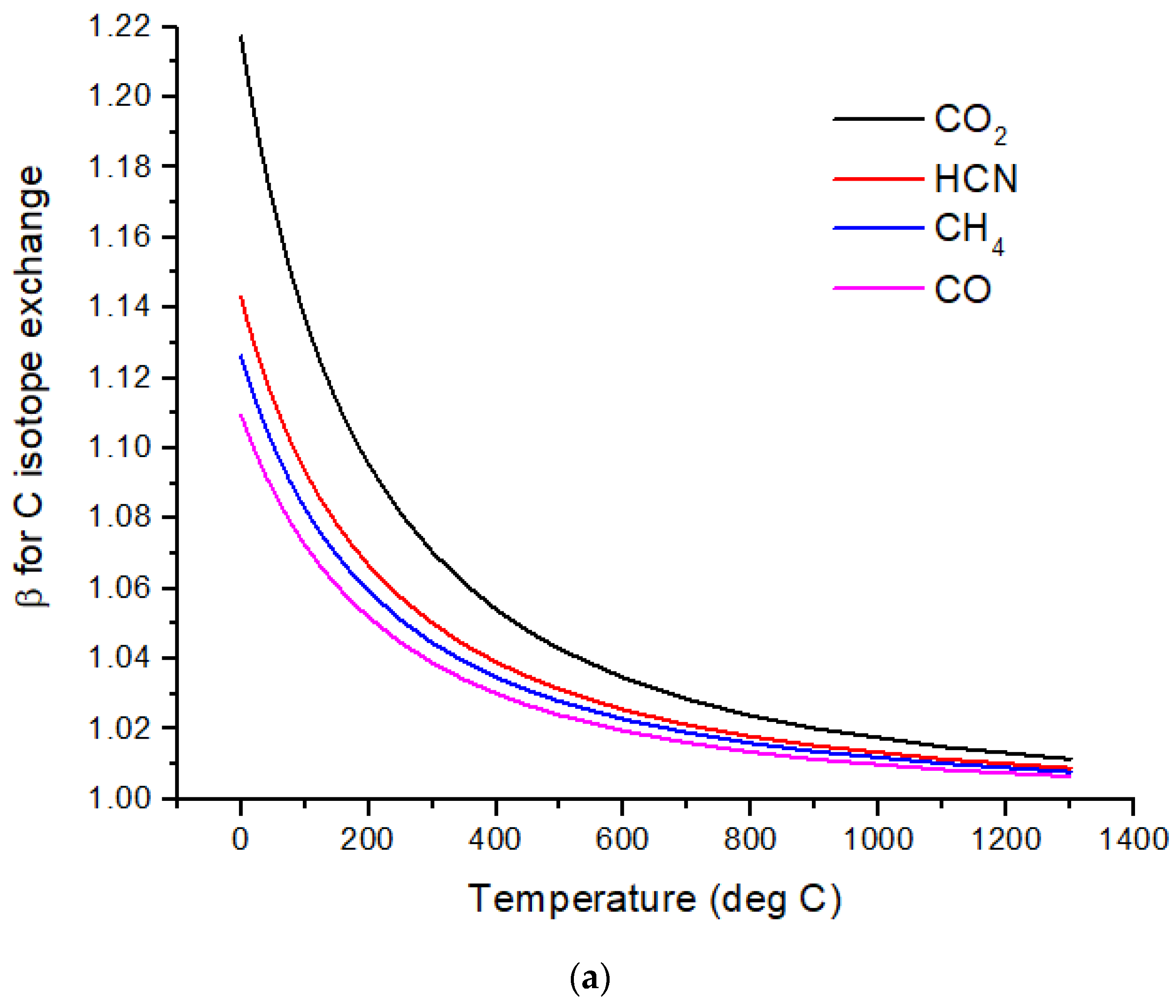
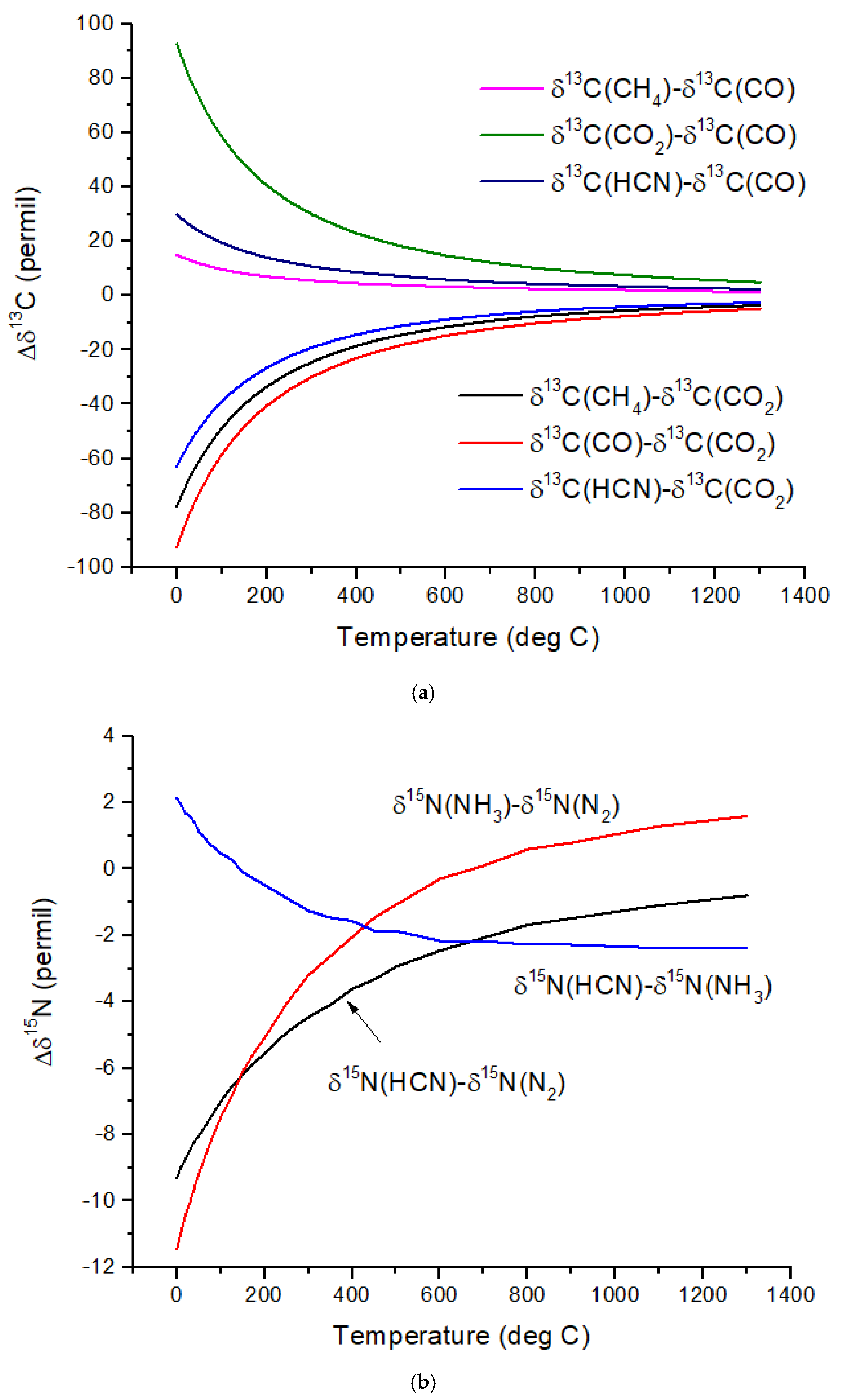
The computed β-factors for C exchange as a function of temperature for CO, CO
2, CH
4, and HCN are shown in
Figure 1a, and the β-factors for N exchange for N
2, NH
3, and HCN are shown in
Figure 1b. The difference in δ
13C values, Δδ
13C, for several pairs of molecules illustrates the expected range of C isotope ratios under conditions of isotopic chemical equilibrium (
Figure 2a). At temperatures above 700 °C, the magnitude of Δδ
13C < 15‰ and decreases with increasing temperature. For hot Jupiters, where CO and to a lesser extent, CO
2 [
35] are the primary carbon-bearing molecules, Δδ
13C is likely to be too small to detect. Isotope-selective photodissociation of CO (i.e., self-shielding) and/or CO
2 will produce non-equilibrium isotope ratios. For hot Jupiters, these effects are primarily in the upper atmosphere. CO self-shielding will produce
13C-depleted CO and
13C-enriched C atoms. If the
13C-rich C atoms are sequestered in a C-rich haze layer, a detectable depletion of
13C in CO may be detectable. If the
13C-rich C is ionized to C
+, rapid isotope exchange with CO will occur, erasing the self-shielding signature. Isotope fractionation due to CO
2 photolysis will occur at longer wavelengths and greater depths in the atmosphere. At greater depths in the atmosphere, C isotope exchange between CO and CO
2 will occur as a result of reactions with H and OH that efficiently inter-convert CO and CO
2.Cooler, rocky exoplanets (T < 500 K) are likely to have N
2 atmospheres with CO
2 or CH
4 as the primary C-bearing molecules [
36]. For temperatures below 400 °C, the magnitude of Δδ
13C > 20‰ relative to CO
2 and increases with decreasing temperature. This well-known equilibrium isotope effect arises from the preference of the heavier isotopes for the higher bond strength compound. For CH
4 in the most common habitable temperature range of 0 to ~50°C, Δδ
13C ~−60 to −80‰ relative to CO
2 at equilibrium. For gases to reach isotopic equilibrium at low temperatures, a catalyst must be present. Life may play the role of a catalyst, although biochemical reactions are generally dominated by kinetic isotope effects.
Nitrogen isotopes do not show as large a range of equilibrium isotope fractionation as the C isotopes (
Figure 2b). At hot Jupiter temperatures, Δδ
15N of only a few permil is predicted for HCN and NH
3 relative to N
2. Even at habitable temperatures, where N
2 is plausibly the primary atmospheric gas (for an Earth-sized planet), Δδ
15N for HCN relative to NH
3 is only ~2‰. These are both astronomically observable molecules, but remotely measuring such a small difference in δ-values is difficult due to the large uncertainties expected for isotope ratio measurements. A small Δδ
15N is consistent with the magnitude of the fractionation that occurs during N
2 fixation by nitrogenase. Measurements by [
37] of δ
15N of biomass produced by diazotrophic growth of several bacterial strains yielded ~−1 to −3‰ relative to air N
2 for traditional bacteria using the most common Mo-Fe nitrogenase. Bacteria using either V-Fe or pure Fe nitrogenase show larger fractionation of −3 to −7‰, but this is still quite small compared to biogenic C isotope fractionation.
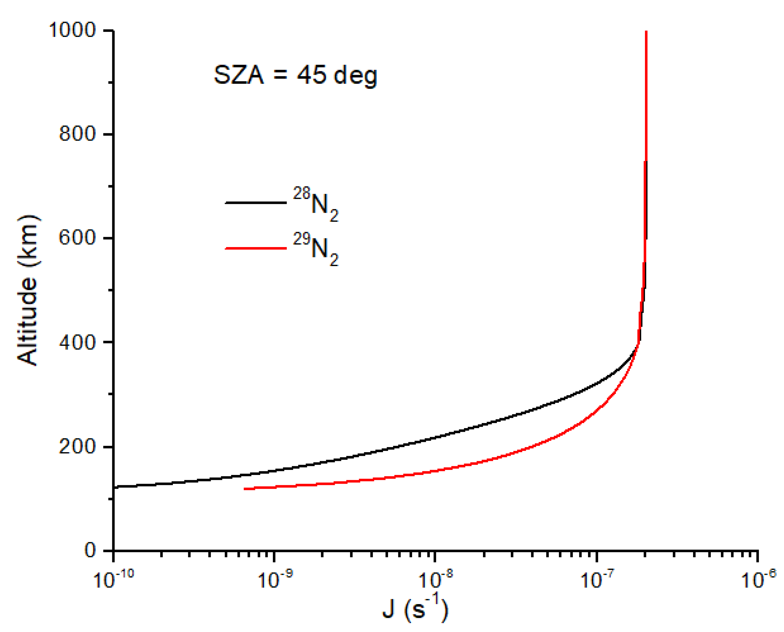
Sulfur isotopes exhibit equilibrium fractionation intermediate between the C and N isotopes (
Figure 2c). Motivated by the photochemical models of Tsai et al. [
37] for WASP-39b, SO
2, H
2S, and S
2 are considered. Other high-temperature S-species include OCS and CS. Of possible relevance to cooler rocky planets, SO
3 and CS
2 δ
34S values are also computed. I have not considered biological fractionation of S isotopes. With an atmospheric temperature of ~900 °C, WASP-39b will have a Δδ
34S ~3‰ for SO
2 relative to H
2S. However, photochemical self-shielding is likely to substantially modify these values, as discussed in the following section.
4. Photochemical Signatures of C, N and S Isotopes
Any assessment of biosignatures in isotope ratios must consider the possibility of photochemically generated signatures. Photochemistry drives atmospheric chemistry away from the thermodynamic equilibrium. If the UV photon flux, atmospheric temperature, and pressure are sufficiently stable, a steady-state photochemical composition will be reached. I consider here how photochemistry can alter the C, N, and S isotope ratios in planetary atmospheres. This is most applicable to terrestrial-type exoplanets, but may have relevance to warm Neptunes and the lower temperature range of hot Jupiters. It is not my intent to exhaustively cover this topic but rather to consider a few specific cases in a qualitative or semi-quantitative manner.
For high-temperature exoplanets, C and N will be present in the IR-detectable region of the atmosphere as primarily CO and N
2. These two diatomic molecules are isoelectronic with the ground states of X
1Σ
+ and X
1Σ
g+, respectively. Both molecules undergo photodissociation in the far-ultraviolet (FUV) region, from 91 to 108 nm for CO and from 91 to 100 nm for N
2 molecules. They are also photodissociated and photoionized at wavelengths <91 nm; however, for H
2-rich environments, the onset of H ionization at 91 nm absorbs most FUV photons, as would be expected for warm Neptunes and hot Jupiters. Both CO and N
2 undergo predissociation, which means that the absorption of a sufficiently energetic FUV photon creates a bound electronically excited state that then either relaxes by fluorescence or crosses to an unbound dissociating state, resulting in atomic products. Again, for both CO and N
2, the bound excited states have relatively long lifetimes (e.g., ~10 psec to 1 nsec), resulting in narrow transition line widths (~0.5 to 0.005 cm
−1). Isotope substitution in these molecules, for example,
13CO and
29N
2, yields an absorption spectrum very similar to the main isotopologues (
12CO and
28N
2) but offset by several to several 10’s of cm
−1. This means that the photodissociation of a column of either CO or N
2 will result in a process termed self-shielding, in which the most abundant isotopologue (
12CO or
28N
2) will become optically thick and cease to dissociate, while the rare isotopologue (
13CO or
29N
2) will continue to undergo photodissociation. The result is a massive enrichment of the rare isotopes of the dissociation products, i.e.,
13C,
15N, or
17O and
18O when considering self-shielding by N
2 or CO, together with a depletion of the rare isotopes in the parent molecules. These isotope effects occur downstream of the region where the primary isotopologues become optically thick in the FUV. Self-shielding is a specific case of isotope-selective photodissociation in which isotope substitution induces changes in the absorption spectrum of a molecule due to changes in the coupling of electronic states. There are numerous examples of molecular clouds, protoplanetary disks [
9,
38,
39], and planetary atmospheres [
14,
40].
I first consider N isotope fractionation due to N
2 self-shielding in the early Earth atmosphere. Photodissociation of N
2 and CH
4 likely produces substantial quantities of HCN [
41,
42], and the self-shielding of N
2 could produce a large
15N enrichment in HCN. As demonstrated by Oro [
43], HCN is an essential ingredient in the prebiotic formation of adenine. To assess this possibility, I use model results from [
42] for the early Earth (0–100 km) combined with an estimate of the downward flux of
28N
2 and
29N
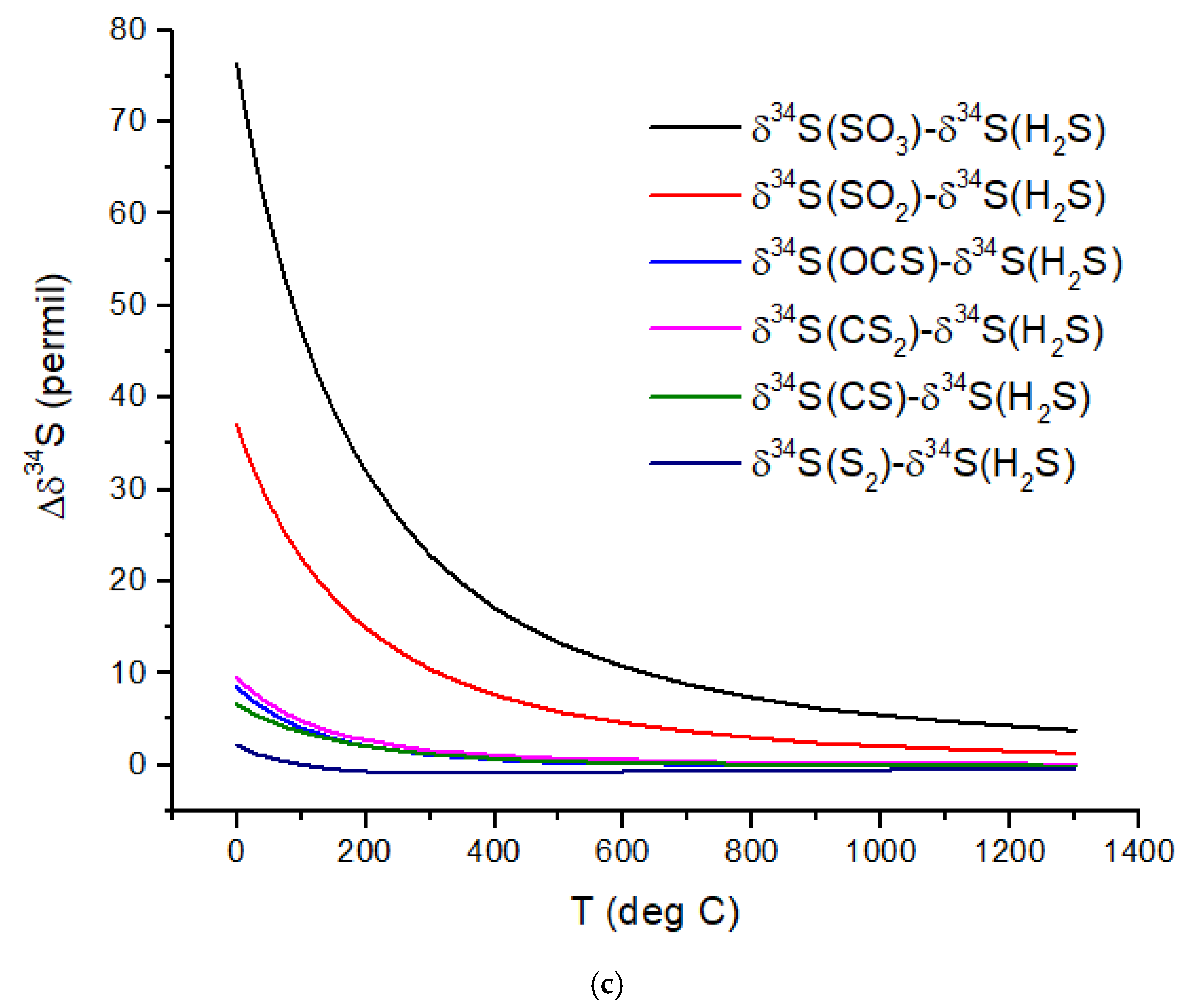
2 from a model of Earth’s upper atmosphere (120–1000 km) (Lyons and Bondoc, in prep). Self-shielding of N
2 occurs primarily at altitudes of 150–300 km. Rather than use the high-resolution cross sections for N
2, I use shielding functions as described in [
38] for CO. Assuming a 45° solar zenith angle and a pure N
2 atmosphere, shielding functions have been determined for self-shielding by
28N
2 and
29N
2, and for mutual shielding by
28N
2 and
29N
2 (on
29N
2 and
28N
2, respectively) [
39]. The photodissociation rate coefficients for
28N
2 and
29N
2 are written as
where Θ
ss and Θ
ms are the self-shielding and mutual-shielding functions,
N is the column density of
28N
2 or
29N
2 from the top of the atmosphere to altitude
z, and
J0 is the N
2 dissociation rate at the top of the atmosphere. Equations (19) and (20) only account for self-shielding from 91 to 100 nm. Although N
2 dissociates down to 80 nm, line broadening makes the self-shielding effect less significant. For the modern atmosphere,
J0 ~2 × 10
−7 s
−1, and for the early Earth atmosphere, it is ~10
3 times higher [
42]. The shielding functions for N
2 are not given here (they are lengthy polynomial expressions) but will be described elsewhere. The photodissociation rate coefficients for
28N
2 and
29N
2 illustrate the self-shielding effect (
Figure 3). At a given altitude between 350 and 120 km,
J29 >
J28 due to self-shielding by
28N
2. The shielding functions in Equations (19) and (20) capture the effects of line saturation in
28N
2 without having to integrate the high-resolution cross sections over wavelength. The decrease in the photolysis rate coefficient for
28N
2 is nearly a factor of 10 at maximal self-shielding altitudes (
Figure 3), yielding
15N enrichment in N atoms of ~1000 permil. In addition to a much higher solar EUV flux, the solar wind particle flux was also much higher, with implications for atmospheric erosion for small, weakly magnetized planets such as Mars [
44], a scenario I will not consider here.
Line broadening will diminish the self-shielding effect. For planetary atmospheres both Doppler and pressure broadening need to be considered. The Doppler linewidth is given by
For the modern Earth thermosphere, the thermospheric temperature is ~1000 K, and the thermal gas velocity (most probable speed) is
vth = 7.7 × 10
4 cm s
−1. At a wavelength of 100 nm, the Doppler linewidth is Δν
D = 0.26 cm
−1. This linewidth is much smaller than the typical spacing between the rotational lines for N
2 and CO and does not impact self-shielding. Pressure broadening derives from the decoherence time due to molecular collisions, and is given by
where σ
c ~3 × 10
−15 cm
2 is the molecular collision cross-section, and
n is the atmospheric number density. At low pressures (<1 microbar), where self-shielding occurs for N
2 in Earth’s atmosphere (
Figure 3), Δν
p ~10
−8 cm
−1, which is negligible.
Photolysis of N
2 produces ground state and excited state atoms in approximately an equal mixture as
N(
2D) decays to N(
4S) with a radiative lifetime of 6.1 × 10
4 s (17 h). It undergoes quenching to N(
4S) by collisions with N
2 and CO on timescales of ~60 s at 100 km in the model from [
42]. N(
2D) can also react with species such as H
2 via the reaction
The model of Tian et al. [
42] has an H
2 mixing ratio of 2 × 10
−3 at 100 km, which implies a loss timescale for N(
2D) by reaction 22 of ~1400 s for a thermosphere temperature of 180 K. All of these timescales are much shorter than the model eddy transport timescale at 100 km of ~3 × 10
5 s. The recombination of N atoms via
acts to reverse the effects of N
2 self-shielding.
A maximum downward flux of
14N and
15N at altitude
z can be estimated by ignoring N loss due to N + NH recombination, which yields
For the modern Earth upper atmosphere model used here,
φ14 = 7.45 × 10
8 cm
−2 s
−1 and
φ15 = 1.76 × 10
7 cm
−2 s
−1 at 120 km. Zahnle [
41] estimates a download N flux of ~1 × 10
10 cm
−2 s
−1 for wavelengths from 79.6 to 91.2 nm. Relative to the modern Earth atmosphere N
2 with
15N/
14N = 1/272.0, the N atom downward flux due to 91–100 nm photons has δ
15N(
φN) = 5400‰. Making the end-member assumption of no self-shielding for 80–91 nm photons, the overall (80–100 nm) δ
15N(
φN) = 370‰. The true value will be between 370 and 5400‰.
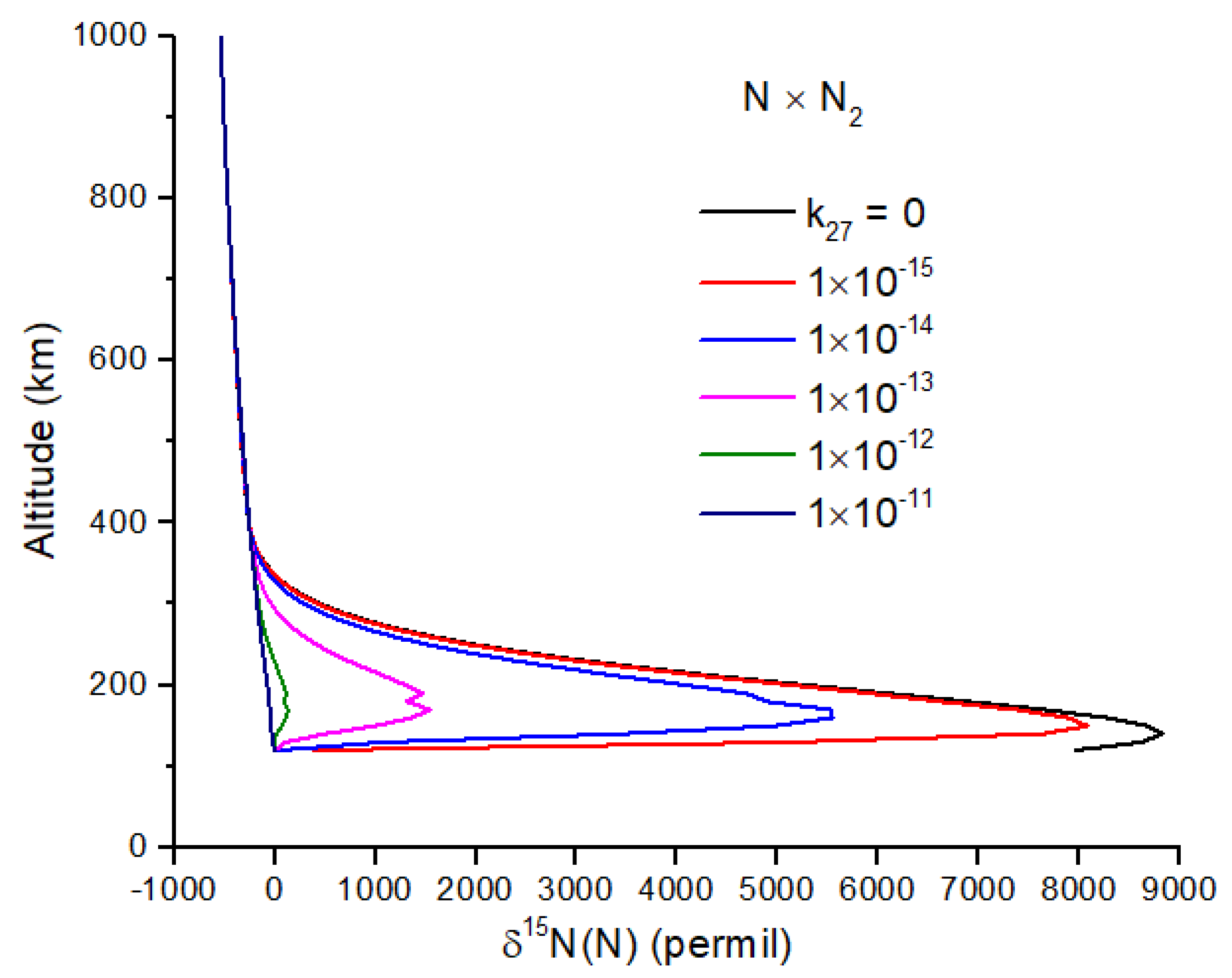
Exchange reactions can also be very important and may include the reactions
For both reactions, the intermediate N
3 is a doublet, and therefore, reaction 27 is spin-forbidden. From the work of [
45], I infer a rate constant of
, which makes reaction 27 negligibly slow at temperatures < 1000 K. If this is not the case, and reaction 27 is important, it will greatly reduce the δ
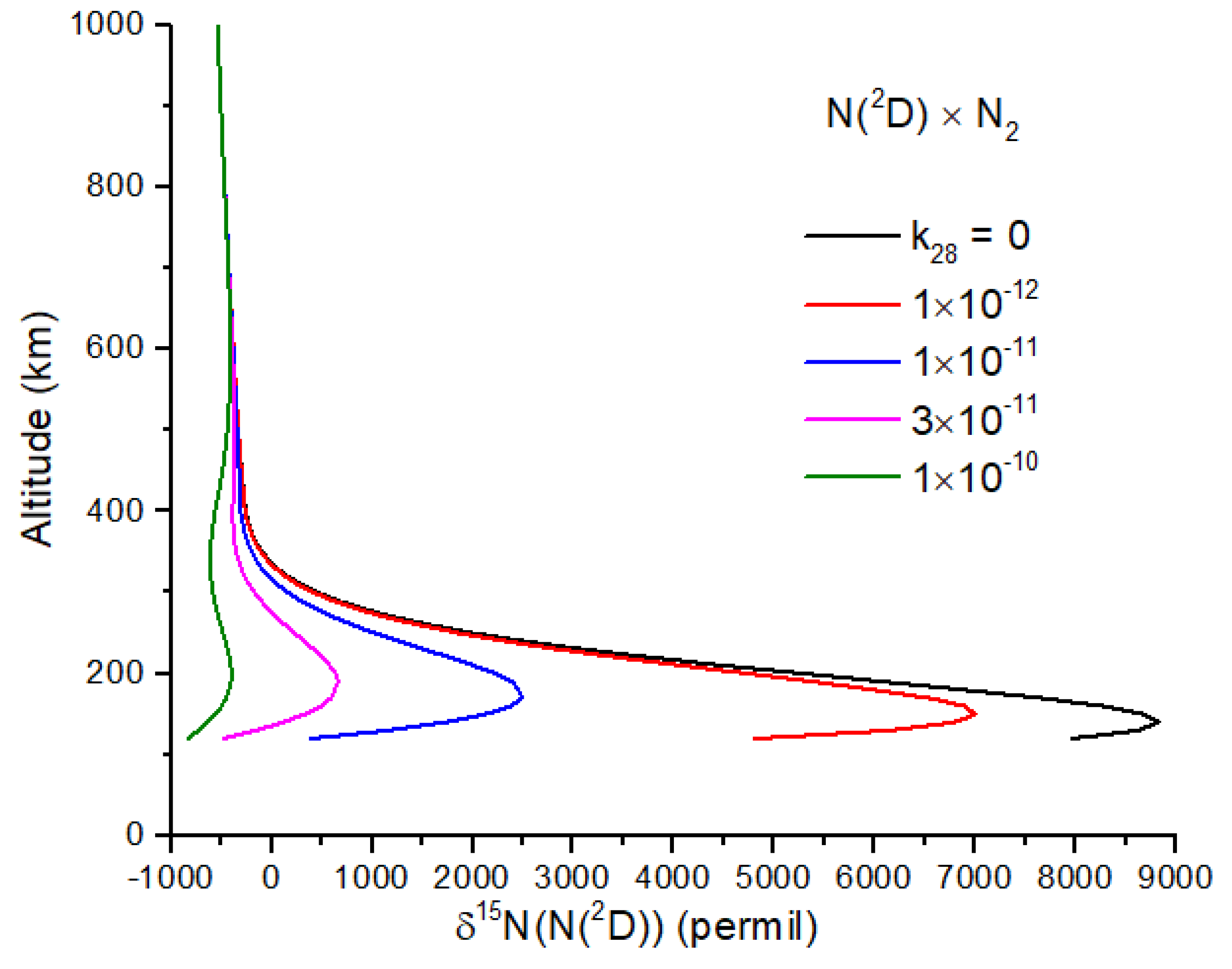
15N enrichment of N atoms (
Figure 4). Reaction 28 is spin-allowed but does not appear to have a measured rate coefficient. At 100 km, the timescale for the loss of
15N(
2D) by reaction 28 is comparable to the timescale for loss by quenching by N
2 for
k28 ~2 × 10
−14 cm
−3 s
−1, a plausible value for a spin-allowed reaction. Further work on reaction 28 is needed, as it too can reduce the N atom δ
15N enrichment (
Figure 5).
HCN is produced by two pathways [
41,
42]
Both of these pathways, which peak at ~70 km in the Tian et al. model [
42], will impart a large
15N enrichment to HCN, specifically δ
15N(HCN) ~370–5400‰ from the results for
φN above. N
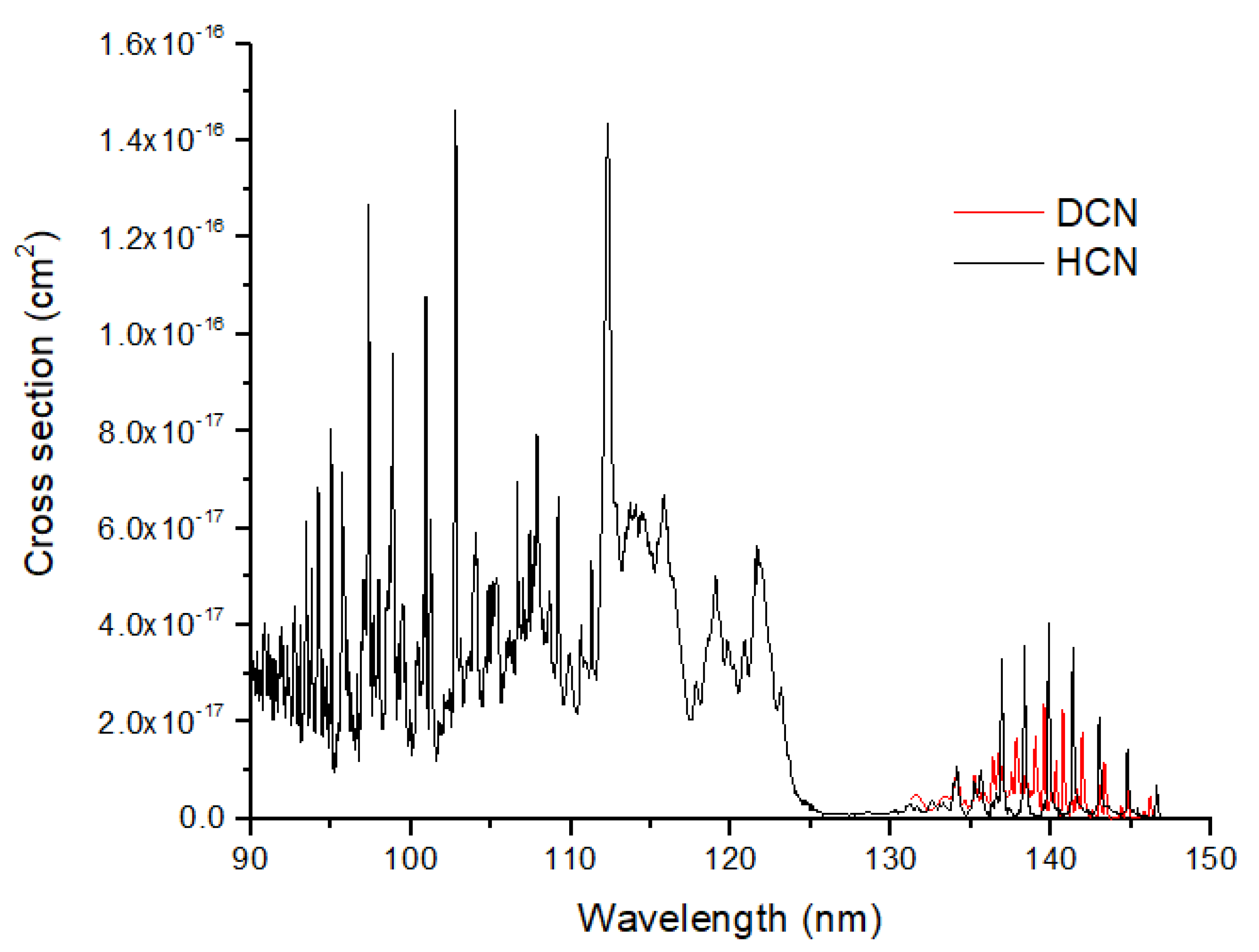
2 self-shielding occurs at considerably higher altitudes (~120–350 km) than does HCN formation. The loss of HCN occurs primarily by photolysis at Ly α (121.6 nm) to make products H + CN. The UV absorption cross sections for HCN show significant structure both near Ly α and in a vibrational progression from 130–150 nm (
Figure 6). The photolysis of HCN is likely to modify the isotope ratios in HCN, as suggested by the large vibrational peak shifts between HCN and DCN. If HCN is optically thick, its
15N enrichment from formation would be reduced. In summary, a significant isotopic photosignature of HCN is a strong possibility for terrestrial-type exoplanets. Because this signature would be enriched in
15N, it should be distinct from any biogenic HCN in the atmosphere. Finally, I note that there is some evidence for
15N enriched Archean organic sediments (e.g., +15‰, ref. [
46]), but these data are from metamorphosed sediments that likely preferentially lost
14N during burial and heating.
Carbon isotopes are also affected by photolysis reactions. The spin-forbidden photolysis of CO
2
was predicted [
47] and experimentally demonstrated [
48] to produce CO with a large depletion of
13C. The large fractionation arises from a small redshift in the absorption spectrum at longer wavelengths for the
13CO
2 isotopologue. The shift occurs in a region of the spectrum that is rapidly decreasing in absorption strength with wavelength, which enhances the effects of the spectral shift. This is also a region of the spectrum populated by hot bands (bands with a lower level vibrational quantum number
v > 0), which makes the isotope fractionation strongly temperature-dependent. There is evidence for this process occurring in the present-day atmosphere of Mars from occultation measurements of CO by the ExoMars spacecraft at Mars, which show that CO has a δ
13C of ~−250 to −150‰ [
49,
50], consistent with CO
2 photolysis as the primary source of CO gas in the Martian atmosphere and consistent with photochemical models [
40].
In Earth’s atmosphere today, CO has a concentration of ~100 ppb and is produced from biomass burning, CH
4 oxidation, and as a byproduct of anthropogenic combustion reactions. ACE-FTS solar occultation measurements of CO in the Earth’s mesosphere reveal isotopically depleted CO at altitudes of ~50–80 km with δ
13C ~−160‰ [
51]. This isotope signature exhibits seasonal and transport-related variations in the mesosphere and upper stratosphere but not in the lower stratosphere and troposphere.
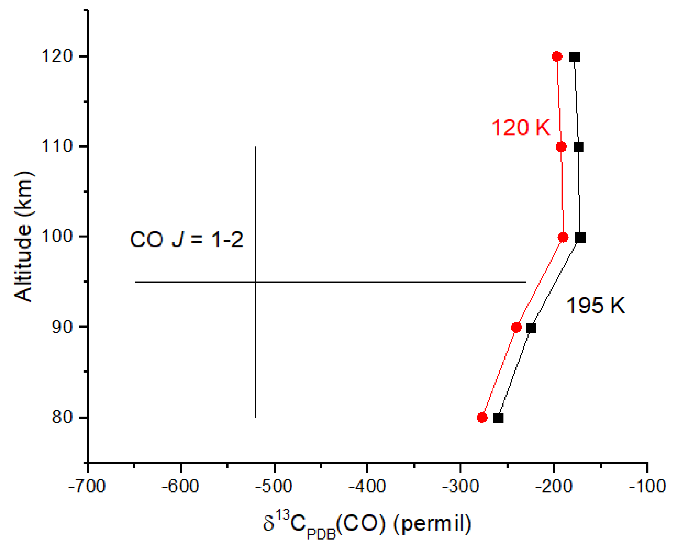
Venus provides another example of a very low δ
13C value for CO in the upper atmosphere. Observations of the
J = 1 → 2 transition for
12CO and
13CO at 230 and 220 GHz in the 80–110 km region of the atmosphere revealed
12CO/
13CO = 185 ± 69 [
52]. Converting this ratio to δ-values relative to the PDB standard yields δ
13C(CO) =
‰. The high end of this range (−230‰) is comparable to those observed on Earth and Mars. I calculated the photodissociation rate coefficients for
12CO
2 and
13CO
2 using equations analogous to Equations (19) and (20) and the ab initio cross sections of [
47] (rather than shielding functions) together with CO
2 number densities from [
53]. Although the measurement uncertainties are large, the
13C depletion in CO is certainly due, at least in part, to reaction 31 (
Figure 7). Ueno et al. [
48] suggest that the cross sections in [
47] overestimate C isotope fractionation by 30%, suggesting that the computed δ
13C values may be too small in magnitude to account for the observations. CO is optically thick up to ~110 km in the Venus mesosphere; therefore, it is possible that
12CO self-shielding at wavelengths <108 nm contributes to the
13C depletion in CO. CO
2 would shield CO at these wavelengths; therefore, CO self-shielding should be diminished. Venus provides an excellent example of a photochemical-derived isotope signature that we can expect in other rocky planets with CO
2 atmospheres.
Of more relevance here is the early Earth atmosphere with a high CO
2 partial pressure and a correspondingly high CO abundance. For the early Earth, ref. [
41] predicts a CO mixing ratio of 2 × 10
−5 at the ground and 1 × 10
−3 at 100 km. The primary source of CO is the photolysis of CO
2 by reaction 31 and at higher altitudes by spin-allowed photolysis of CO
2 at wavelengths <167 nm (which does not cause large isotope fractionation). As CO
2 photolysis is the primary source of CO, a large negative δ
13C signature is expected to be present in the middle atmosphere. The reaction
, a primary loss pathway for CO, will act to decrease the
13C enrichment in CO. The net result is a low δ
13C value (~−100 to −200‰) for CO in the middle atmosphere, which may eventually be detectable in analogous rocky exoplanets using cross-correlation techniques.
I next briefly consider C isotope fractionation due to CO self-shielding in the early Earth atmosphere and in an H2-rich exoplanet atmosphere. CO will be optically thick and, therefore, undergo self-shielding at a lower altitude than N2 because of its lower abundance. Because both molecules have long-lived predissociation states, the mutual shielding of N2 on CO will occur but will not significantly diminish the self-shielding in CO. I therefore expect large 13C and 17O and 18O enrichments in product C and O atoms. The fates of C and O atoms differ. C is likely to react with OH to reform CO via C + OH → CO + H, which would act to reverse the effects of CO self-shielding. If an organic haze is present, 13C-enriched C could be sequestered in the haze, leaving measurable 13C-depleted CO in the atmosphere. Isotopically enriched O atoms are likely to eventually form H2O, although the initiating reaction, O + H2 → OH + H, is strongly temperature-dependent. Exchange reactions between O and O2 and OH and H2O will diminish the self-shielding signature in O isotopes, but a positive δ17O and δ18O in atmospheric H2O is possible, although it is likely to be diluted by H2O already in the atmosphere.
I next consider CO self-shielding in a warm Neptune/hot Jupiter. At very high temperatures, isotopically enriched O will rapidly form OH and H
2O, and the reaction OH + CO → CO
2 + H and the reverse reaction will act to erase the self-shielding signature in O-containing species. In addition, the exchange reaction
which has an activation energy of 6.9 kcal mole
−1 (activation temperature of 3470 K), will also reduce the self-shielding signature. The fate of the
13C-enriched C atoms is less clear. C may react with H
2 to form CH
2 in the 3-body reaction
where M is a 3rd-body molecule (H
2 most likely). The rate constant is 6.9 × 10
−32 cm
6 s
−1 at 300 K [
54], and is likely somewhat slower at higher temperatures. This reaction is too slow at CO self-shielding altitudes, which are likely to be ~microbars of total pressure. Radiative recombination,
, is likely a faster pathway with a typical rate constant of ~1 × 10
−12 cm
3 s
−1, and thus a loss timescale for C of ~1 s. The formation of
3CH
2 would lead to CO reformation via reactions such as
, or more indirectly by
followed by the reaction of CH with O to form CO. Reformation of CO by any of these reactions will decrease the magnitude of the self-shielding signature in C. Another possible mechanism for erasing a CO self-shielding signature is the exchange of C with CO via
This reaction should proceed through a C
2O intermediate with a triplet ground state, which is spin-allowed. I did not find a 2-body exchange rate coefficient for reaction 33; however, there is a measured 3-body rate coefficient for C
2O formation of 6.31 × 10
−32 cm
6 s
−1 [
55].
If C produced from CO photolysis under self-shielding conditions avoids recombination to CO, one possible fate for it would be to form a haze layer, either by contributing to an existing organic haze layer or by forming a solid carbon haze layer at high altitudes via the reaction (s). Depending on the temperature, C particles can condense as either amorphous carbon or graphite. The haze particles would be 13C-enriched, and the CO would be 13C-depleted at altitudes in the vicinity of the CO self-shielding. The latter may be detectable at infrared wavelengths, as a low 13C/12C ratio.
Finally, I briefly consider the sulfur isotopes in hot Jupiters. The detection of photochemically produced SO
2 in the hot Jupiter WASP-39b [
37] provides the prospect of measuring the exoplanet
32S/
34S isotope ratio modified by UV self-shielding. Self-shielding in SO
2 has been investigated as a mechanism for explaining Archean S isotope signatures in sedimentary rocks [
56,
57]. SO
2 undergoes predissociation in the C-X band from about 180–220 nm and has an absorption spectrum with resolved lines in a vibronic progression. Sulfur isotope substitution creates a redshift in this spectrum, which generates a large isotope enrichment of the less abundant stable isotopes (
34S,
33S, and
36S) in the dissociation product SO. Although this mechanism does not explain the early Earth rock record, it has been verified experimentally [
58]. The key requirement is an optically thick column of SO
2.
For WASP-39b, the peak mixing ratio for SO
2 is ~5 × 10
−5 at ~0.1 mbar on the morning terminator and ~2 × 10
−5 at ~0.03 mbar on the evening terminator [
37]. For a scale height of 890 km, these correspond to vertical column densities of 2.9 × 10
18 cm
−2 and 3.9 × 10
17 cm
−2 in the morning and evening, respectively. The peak cross-section for SO
2 near 200 nm is ~3 × 10
−17 cm
2 at room temperature and ~2 × 10
−17 cm
2 at ~1000 K. (It should be noted that the absorption lines are narrow; therefore, accurate UV cross sections require high-resolution laboratory measurements). Peak vertical optical depths are ~58 and 7.8, morning and evening. The tangential optical depths along the terminators are ~25 times the vertical optical depths. Thus, at the peak SO
2 mixing ratios, SO
2 is strongly optically thick under all conditions. Self-shielding by
32SO
2 will produce a large enrichment in
34SO during photolysis
where
x = 32 or 34 (and also 33 and 36, but these are much less abundant). Self-shielding by
32SO
2 means that
J34 >>
J32, so the instantaneous number density of
34SO will be highly enriched compared to the standard isotope ratios. (The sulfur isotope standard is a meteorite mineral, the Canyon Diablo troilite or CDT). Models [
56] and measurements [
57,
58] suggest δ
34S ~100 to 200‰ enrichments in SO. The steady-state enrichment of
34SO and the corresponding depletion of
34SO
2 depend on subsequent and concurrent reactions. SO and SO
2 are produced by oxidation reactions with OH, which is produced by the photolysis of H
2O [
37]. Although photolysis is the primary loss process for SO
2 in WASP-39b, the continual reformation of SO and SO
2 will act to reduce the self-shielding signature. Additionally, S exchange with SO,
may also reduce the self-shielding enrichment of
34SO unless SO photolysis is the primary source of S atoms. Detailed photochemical modeling is required to address these issues.
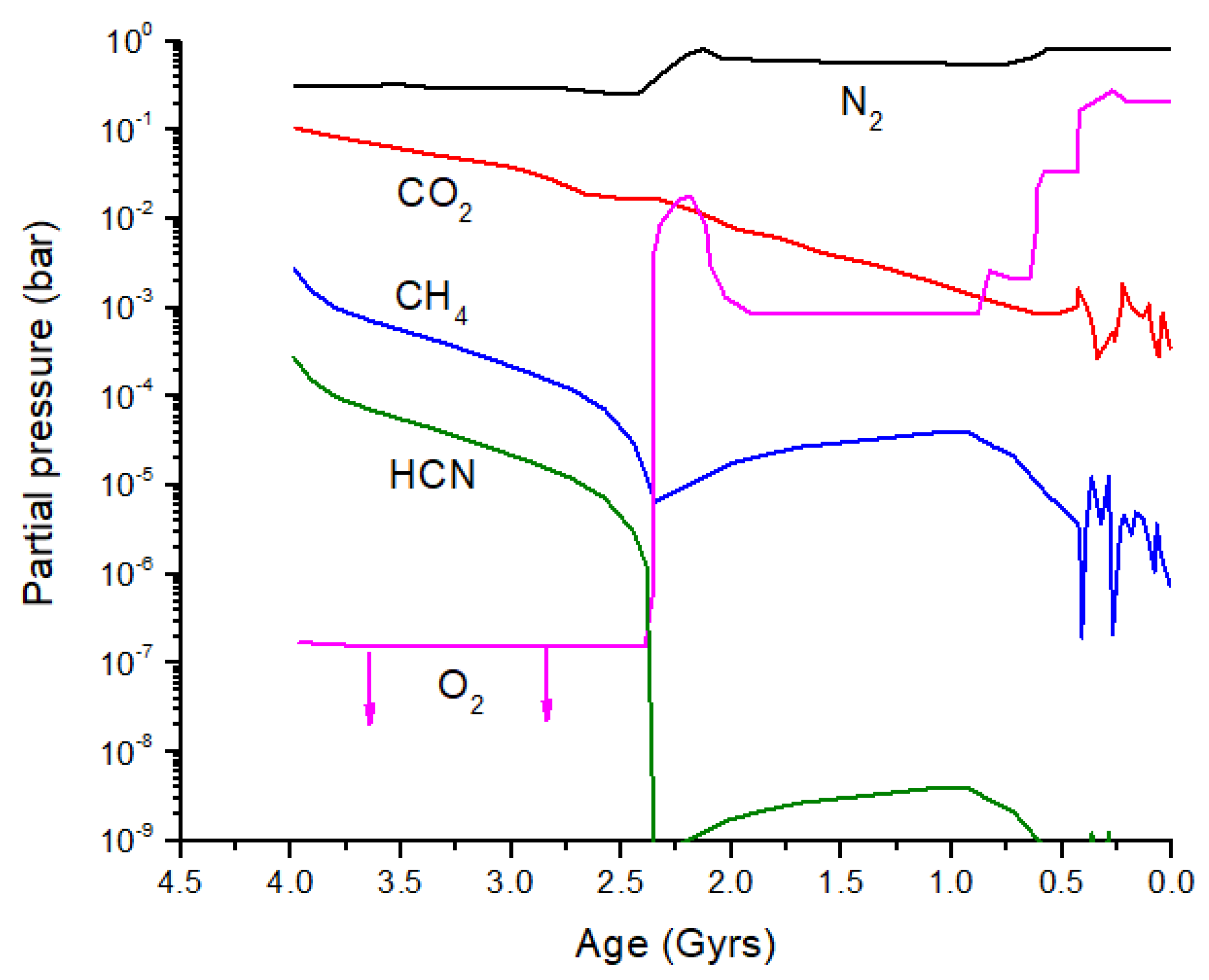
5. Evolution of C and N Isotopes in Earth’s Early Atmosphere
From the discussion above, it is clear that significant isotope fractionation is possible in exoplanet atmospheres. Is it possible to see biosignatures against this backdrop of equilibrium and photo-induced isotope fractionation, and what might this have looked like in early Earth? Catling and Zahnle [
2] produced an evolution diagram of the composition of Earth’s atmosphere over the past 4 billion years (
Figure 8). I have added HCN to this diagram by scaling HCN relative to CH
4 before and after the atmospheric Great Oxidation Event (GOE): 10
−1 prior to the GOE and 10
−4 after the GOE. More accurate HCN evolution calculations can be performed. Prior to the GOE, the primary loss process for HCN is photolysis; after the GOE, loss by OH dominates, although the rate of this loss reaction will vary depending on the O
3 partial pressure.
Catling and Zahnle [
2] assumed a gradual onset of methanogenesis at ~4.0 Gyr and a gradual onset of photosynthesis at ~3.0 Gyr. Thus, in their model, the high CH
4 partial pressure (2000 ppm) at 4.0 Gyrs may be mostly biogenic. Prior to the onset of methanogenesis, but after the short-lived massive impact-generated reduced atmospheres, CH
4 is primarily thermogenic and/or derived from geothermal and hydrothermal reactions. Thermogenic refers to CH
4 produced by the high-temperature decomposition of buried organic compounds. Today and during the Phanerozoic, most buried organics are biogenic in origin; therefore, the δ
13C values for atmospheric CH
4 are relatively low at ~−20 to −50‰ (
Figure 9) [
59]. Prior to 4.0 Gyrs, most buried organics were either derived from the original delivery of chondritic materials or from the burial of material produced by the UV processing of impact-reduced atmospheres. Bulk insoluble organic matter (IOM) in carbonaceous chondrites has δ
13C ~−35 to −10‰ and in ordinary chondrites has δ
13C ~−24 to −10‰ [
60], coincidentally similar to the range for C
3 and C
4 plants. It is therefore likely that thermogenic CH
4 produced from 4.4 to 4.0 Gyr would have a similar range of δ
13C values to what we see today (
Figure 9).
Geothermal and hydrothermal CH
4 differ from thermogenic CH
4 in that the former is derived from inorganic reactions in the Earth’s crust. The general form of the reaction responsible for the geothermal/hydrothermal production of CH
4, known as the Sabatier reaction, is
[
61]. Serpentinization, which generates H
2 in the crust via a redox reaction between Fe(II) and H
2O, also falls into this category of reactions. I will not assess the possible flux of CH
4 prior to methanogenesis, but I will assume that the flux of CH
4 available from crustal sources was sufficient to maintain a substantial CH
4 partial pressure.
Following Catling and Zahnle [
2], I assume that methanogenesis becomes the dominant CH
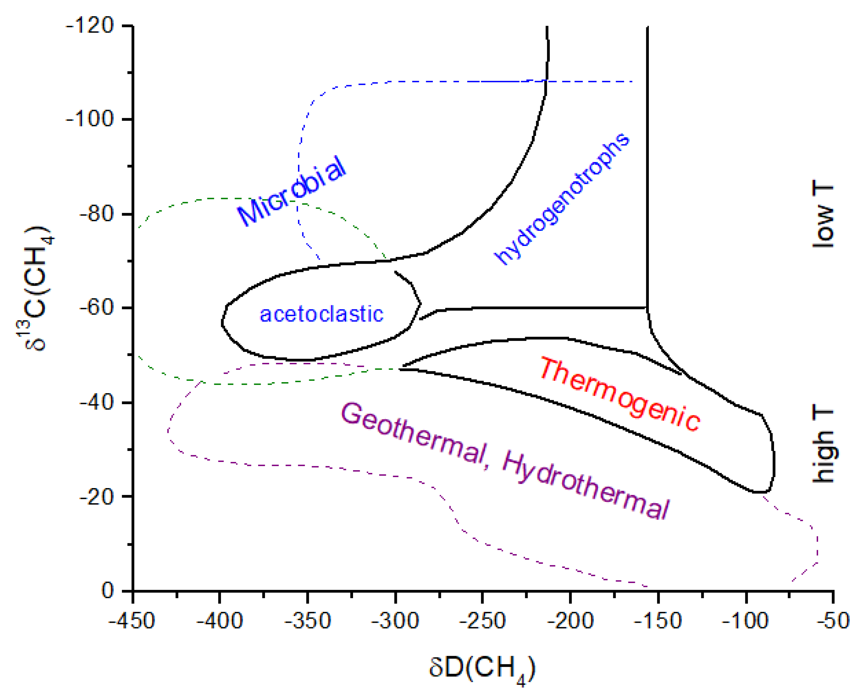
4 source by ~4.0 Gyr. If hydrogenotrophic methanogenesis is the primary initial methanogenic process (
Figure 9), then substantial
13C depletion is likely to be present in atmospheric CH
4 (
Figure 10). If acetoclastic methanogenesis was the primary source of CH
4, then atmospheric CH
4 would have been less strongly fractionated. Carbon isotope analysis of organics in ancient rocks yields a mean of δ
13C ~−30‰ with a large variation [
62] (
Figure 10). If hydrogenotrophic methanogenesis was the predominant source of CH
4 in the ancient atmosphere, then the organics in rocks have δ
13C values decoupled from atmospheric CH
4. Anaerobic methane oxidation by methanotrophs, which is known to produce extremely light δ
13C in lipids (<−100‰) and leave correpsondingly
13C-enriched CH
4, could also modify the CH
4 δ
13C history, as shown in
Figure 10. In the modern atmosphere, anaerobic methanotrophy does not significantly alter δ
13C for atmospheric CH
4 (see
Section 2). For the early Earth, it has been argued that anaerobic methanotrophs can explain Tumbiana Formation organics with δ
13C ~−60‰ at 2.8 Gyr ago [
63] (not shown in
Figure 10). This event could have produced atmospheric CH
4 with δ
13C values of >>−50‰. Given the above considerations, the evolution of methanogenesis and δ
13C for atmospheric CH
4 in
Figure 10 must be treated as an approximation of the actual values.
The reservoir of dissolved inorganic carbon (DIC) in the oceans today is ~38,000 Pg C, vastly larger than the sum of atmosphere, land plants, and soil C, which is ~2800 Pg C [
22]. Even for a slightly more acidic early ocean, C would be present primarily as HCO
3− and CO
32−, and I assume that δ
13C of early DIC is approximately the same as modern DIC. I make this assumption because air-sea exchange is the primary source of equilibrium fractionation between atmospheric CO
2 and DIC [
21]. Photosynthesis in surface waters creates additional
13C enrichment in DIC and yields δ
13C(DIC) ~+1 to + 3‰ [
64]. The majority of carbonates in sedimentary rocks are believed to be biogenic, and the δ
13C of carbonates has generally been fairly close to 0‰ over the past 3.5 Gyrs, with occasional deviations of ±10‰ [
65]. I will further assume that abiotic carbonate formation on the prebiotic Earth did not strongly affect the C isotope ratios in atmospheric CO
2, while CO
2 mostly tracked marine carbonate formation over the past 3.5 Gyrs with a roughly constant fractionation due to air-sea exchange.
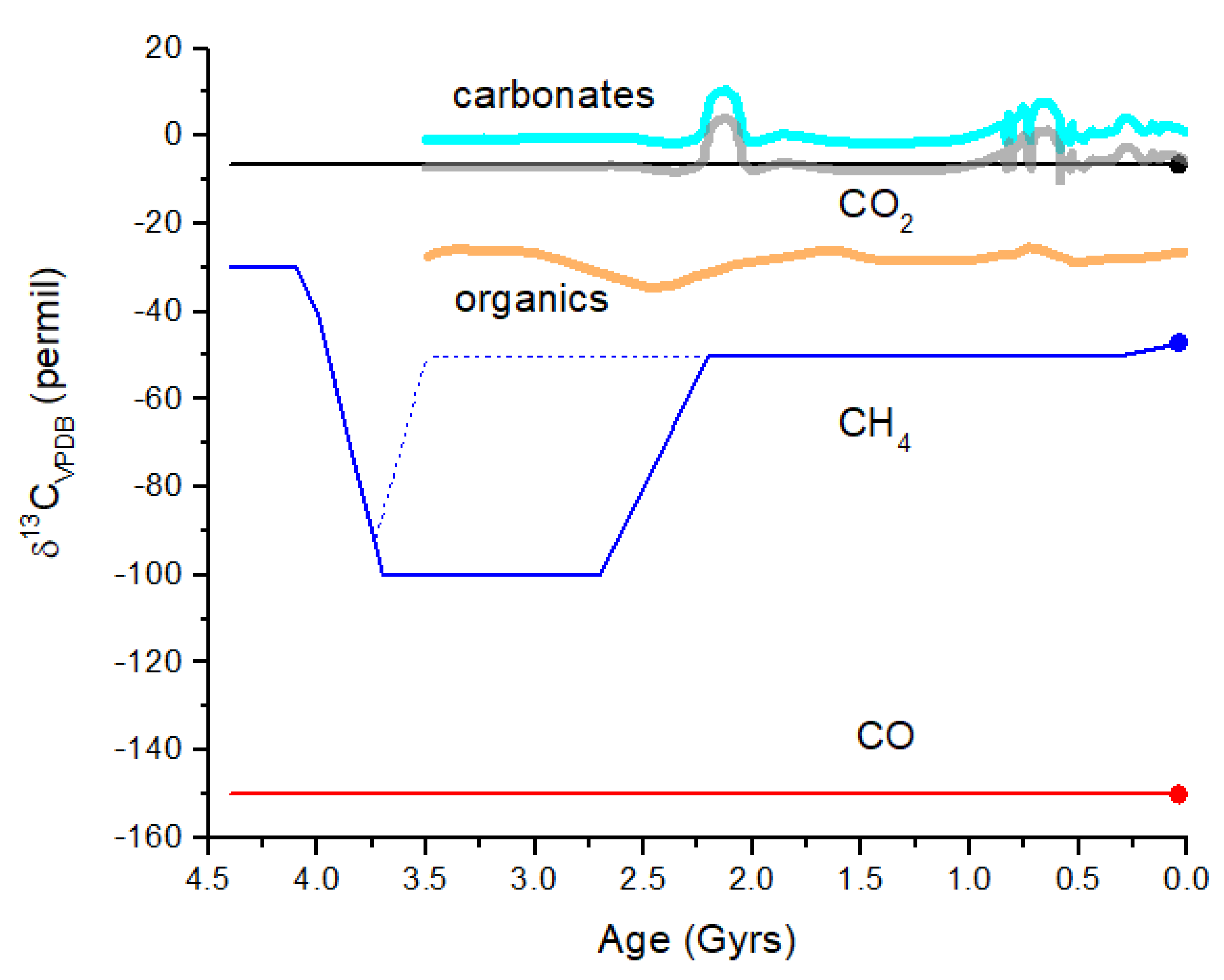
Figure 10 illustrates the evolution of δ
13C for CO
2 over the past 4.4 Gyrs, with the constant value of −6.5‰ [
64] prior to 3.5 Gyr ago supplanted by the curve (thick gray line) that tracks the carbonates. The CO curve represents the minimum δ
13C expected due to CO
2 photolysis. This minimum occurs at a high altitude in the mesosphere or even the lower thermosphere for a high
pCO
2 case. In the lower atmosphere, the δ
13C of CO is closer to that of CO
2.
Figure 10.
Schematic representation of δ
13C evolution in the Earth’s atmosphere. In the simplest scenario, CO
2 is derived from volcanism and has δ
13C ~−6.5‰ as for mantle C. CO
2 undergoes gas exchange with the surface ocean throughout Earth history since 4.4 Gyr ago (black line). More likely, CO
2 tracked the carbonates. The carbonates curve (thick cyan line) is a smoothed version of measurements of δ
13C for marine carbonates over the past 3.5 Gyr [
65]. The curve illustrates the approximate range of variation seen in marine carbonates, which would likely be present in atmospheric CO
2. Atmospheric CO
2 will track carbonates but will be displaced by about −6.5‰ (thick gray curve). The CO curve illustrates the effect of isotope fractionation during CO
2 photolysis in the upper atmosphere. Although δ
13C for CO is constant over time, the CO mixing ratio decreases by many orders of magnitude from ~10
−3 at 4 Gyr to ~10
−10 today. The CH
4 curve (blue line) illustrates abiogenic sources prior to 4.0 Gyr ago, followed by hydrogenotrophic methanogenesis for the next ~1.5 Gyr, and then CH
4 with modern δ
13C values after the GOE at 2.4 Gyr ago. The mean δ
13C for organics recorded from rocks (thick orange line) [
62] does not exhibit highly negative δ
13C, indicating that either the rock record does not entirely correlate with atmospheric CH
4 or that methanogenesis was not a major biochemical process (dotted blue line). The δ
13C difference between CO
2 and abiogenic CH
4 is ~25‰ versus ~95‰ between CO
2 and hydrogenotrophic methanogen CH
4. This comparison of CO
2 and CH
4 may represent a viable biosignature in a given terrestrial exoplanet atmosphere.
![Life 15 00398 g010]()
From
Figure 10, the maximum difference in δ
13C for atmospheric CH
4 and CO
2 is Δδ
13C = δ
13C(CH
4) − δ
13C(CO
2) ~−95‰ during an era when hydrogenotrophic methanogenesis was dominant. In the modern atmosphere, this difference is about −40‰, and in the prebiotic atmosphere, this difference may have been ~−25 to −30‰. For Earth-like exoplanets (i.e., rocky planets with oceans), the value of Δδ
13C may serve as a biosignature, assuming similar microbial evolution. Δδ
13C is an entirely internal measure, meaning that a comparison with the δ
13C of the parent star or other objects in the planetary system is not necessary. The feasibility of measuring Δδ
13C in an exoplanet atmosphere is considered in the following section.
6. Spectral Signatures of Isotopic Gases
Here, I briefly consider the HITRAN line intensities [
66] for the relevant isotopologues discussed above to illustrate the magnitude of the isotope-induced band shifts. A complete analysis of the detectability of the isotope ratios discussed above should include isotopologue cross sections, line broadening, and detection in a noisy spectrum [
4,
67], which will be discussed elsewhere.
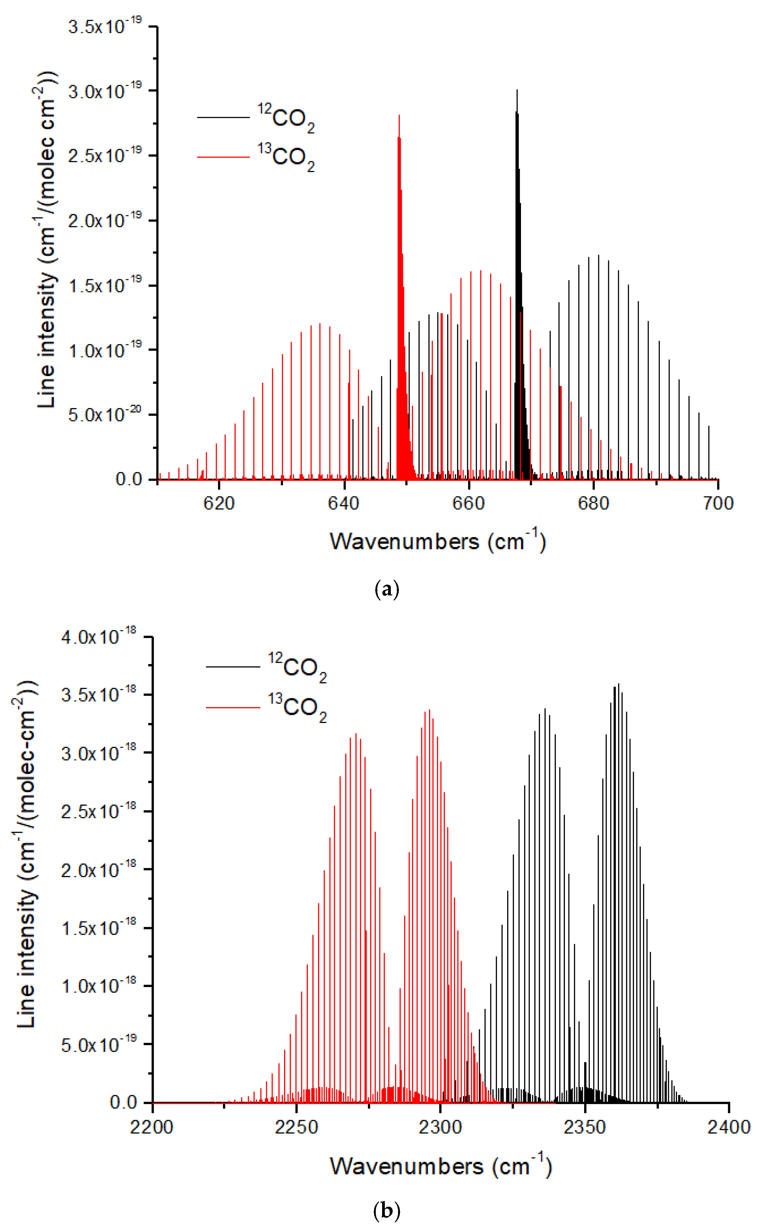
The ν
2 and ν
3 bands of CO
2 show redshifts of 19 cm
−1 and 70 cm
−1, respectively, for the
13CO
2 isotopologue (
Figure 11). These large redshifts reflect the large displacement of the C atom in the bending and asymmetric stretch modes of CO
2. As discussed in [
16], the large band shifts in CO
2 make isotopologue ratio measurements possible in exoplanet atmospheres with large atmospheric scale heights using JWST MIRI or NIRSpec at medium spectral resolution (
R ~1000–3000). The CO molecule [
66] also exhibits large isotopic band shifts of ~50 cm
−1 and ~95 cm
−1 for the fundamental (4.7 microns) and first overtone (2.35 microns). CO is especially useful for measuring isotope ratios in hot Jupiters [
6] and brown dwarfs [
7], and is essential for determining the C isotope ratio of the solar photosphere [
13]. In addition, CO is the molecule of choice for measuring the C and O isotope ratios in exoplanet parent stars.
Figure 11.
(
a) Normalized line intensities at 296 K for the ν
2 band (bending mode) of
12CO
2 and
13CO
2. The redshift of the
13CO
2 spectrum is ~19 cm
−1. (
b) For the CO
2 ν
3 band (asymmetric stretch) the redshift is larger at ~70 cm
−1. For both figures, the
13CO
2 line intensity has been normalized by the
13C fraction (0.011057) given in HITRAN. Data were obtained from HITRANonline [
66].
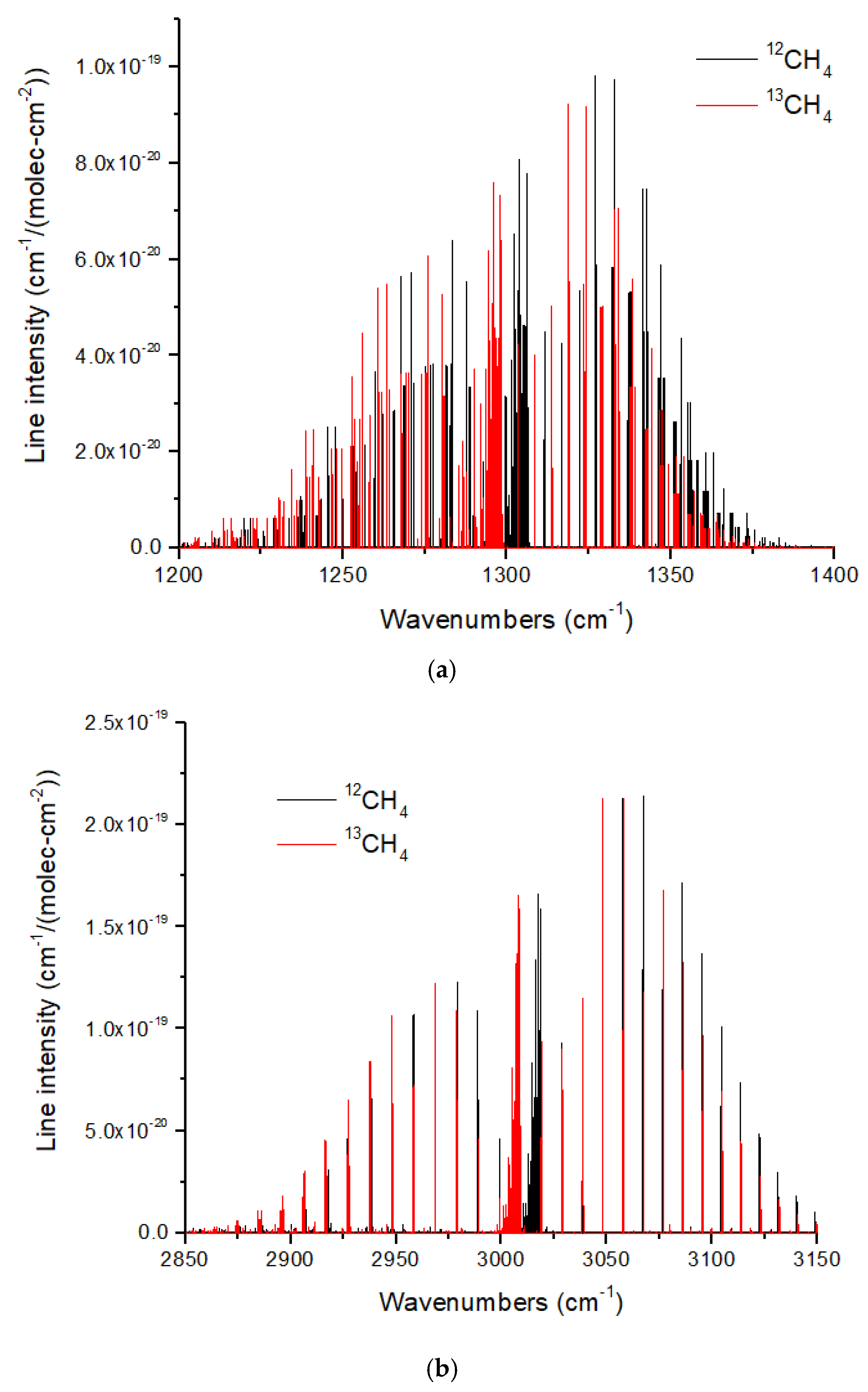
The ν
3 (3.3 microns) and ν
4 (7.7 microns) bands of CH
4 also show redshifts upon
13C substitution. However, these redshifts are ~8–10 cm
−1 (
Figure 12), which are smaller than those for CO and CO
2. In addition, there is an occasional overlap in the ν
4 band. This means that some
13CH
4 lines will be masked by lines from the ~100 times more abundant
12CH
4. This problem is more acute for the ν
3 band, for which there is a coincidental overlap of the P and R branch lines adjacent to the Q-branch, such that pressure broadening will cause increased line overlap and masking of
13CH
4. The Q branches of both bands are a complex cluster of lines with a typical line spacing of ~0.05–0.10 cm
−1. Resolving these lines would require a high spectral resolution of
R ~30,000–60,000, far beyond the JWST capability. Resolving the Q-branch envelopes is easier, requiring a minimum
R ~160 and 380 for ν
4 and ν
3, respectively.
As discussed above, HCN photochemically produced in a N
2-CO
2-CH
4 atmosphere, as proposed for the Archean Earth, is expected to have a massive
15N enrichment (δ
15N ~300 to several 1000‰) due to N
2 self-shielding at wavelengths <100 nm. HCN is a linear molecule with a C-H stretch mode (ν
1), a doubly degenerate bending mode (ν
2), and a C-N stretch mode (ν
3). Only the ν
3 mode has substantial N displacement, but it is a very weak band. The much stronger ν
1 and ν
2 bands have substantial C displacement but only slight N displacement (
Figure 13a). The result is a very small ν
2 band shift of ~1–1.5 cm
−1 for HC
15N, causing overlap between the Q branches (
Figure 13b). To resolve these Q branches requires a minimum resolution of
R ~700, and to resolve individual lines requires
R ~3500–7000. Hydrogen isocyanide, HNC, with a central N atom, will exhibit larger band shifts for H
15NC, although it is generally less abundant than HCN.
As a final spectroscopic example, I consider
32SO
2 and
34SO
2. The SO
2 ν
3 band at 1360 cm
−1 is strong and exhibits a band shift of 18 cm
−1 (
Figure 14a). The spectrum is densely populated with transitions, which means that the line overlap from
32SO
2 may shield some of the
34SO
2 lines. Line overlap is an important consideration when retrieving the isotope ratios. Significant line overlap by the more abundant isotopologue will create an artificially low abundance for the rare isotopes in this case,
34SO
2. This could give the impression of a stronger self-shielding signature in SO
2 than is actually present. The typical spacing between the lines can be assessed from
Figure 14b. The line spacing for a given isotopologue for ν
3 is ~0.03 to 0.2 cm
−1, which requires a spectral resolution of
R ~6700–45,000.
Model calculations by Tsai et al. [
37] suggest that SO may also be observable in WASP-39b or similar atmospheres. HITRAN does not have line intensity data for
34SO, but estimating the fundamental vibrational frequency from the
32SO fundamental gives
where μ is the reduced mass of each isotopologue. For ν
32 ~1125 cm
−1, ν
34 ~1114 cm
−1 for a red shift of 11 cm
−1. Reaction 34 will result in a significant enhancement of
34SO, which, together with the less dense SO spectrum, suggests that it may be easier to obtain a S isotope ratio from SO than from SO
2.


