

Abiotic and Herbivory Combined Stress in Tomato: Additive, Synergic and Antagonistic Effects and Within-Plant Phenotypic Plasticity


 ,
, 
 and
and 
Abstract
1. Introduction
2. Materials and Methods
2.1. Experimental Procedure and Plant Material
2.2. Tomato Growth Conditions
2.3. Insect Rearing
2.4. Abiotic Stress and Herbivory Treatment
- (1)
- two hydroponic units were renewed with the optimal nutrient solution (CTR group);
- (2)
- two hydroponic units were renewed with the nutrient solution with N deficiency and PEG (ABIO group);
- (3)
- two hydroponic units received the optimal nutrient solution but the plants were infested with Tuta larvae to induce the biotic stress (BIO group);
- (4)
- two hydroponic units maintained the same nutrient solution with N deficiency and PEG and, in addition, the plants were infested by Tuta larvae (COMB group).
2.5. First Experimental: Synergic, Antagonistic and Additive Effects
2.5.1. Tomato Samplings and Measurements
2.5.2. Gas Exchange Measurements
2.5.3. Morphological Measurements
2.5.4. VOCs Analysis
2.5.5. Statistical Analysis
Morpho-Physiological Data
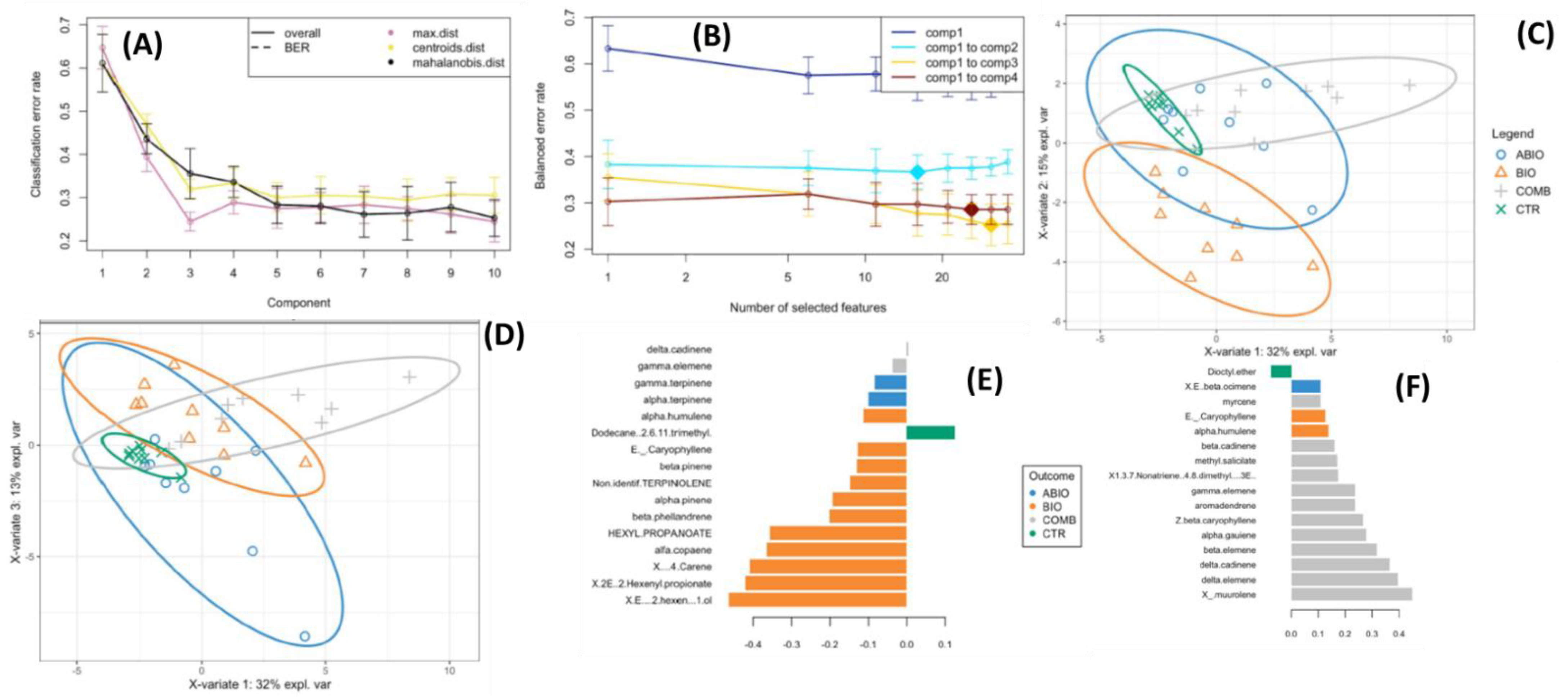
VOCs Data
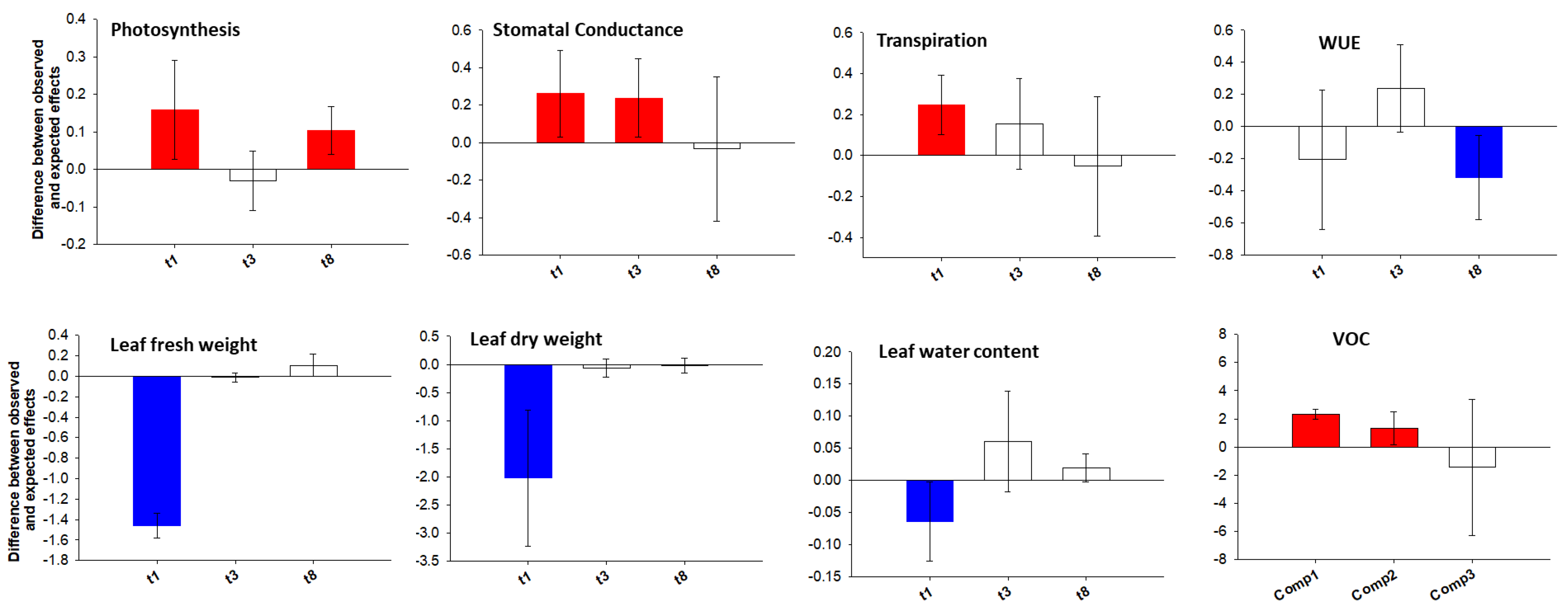
Calculation of Additive, Synergistic or Antagonistic Effects in Combined Stress
2.6. Second Experiment: Within-Plant Phenotypic Plasticity
2.6.1. Tomato Samplings and Measurements
2.6.2. Statistics
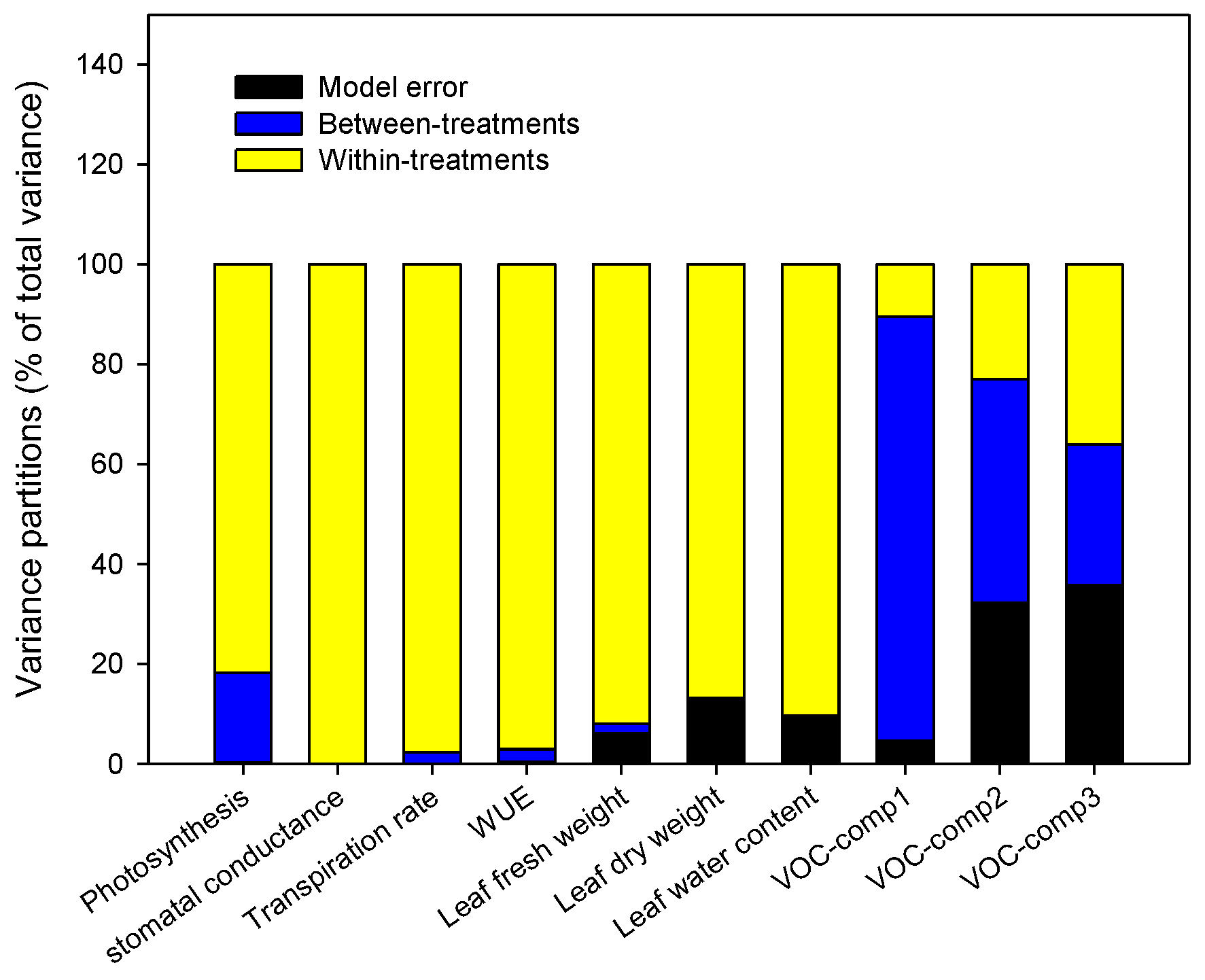
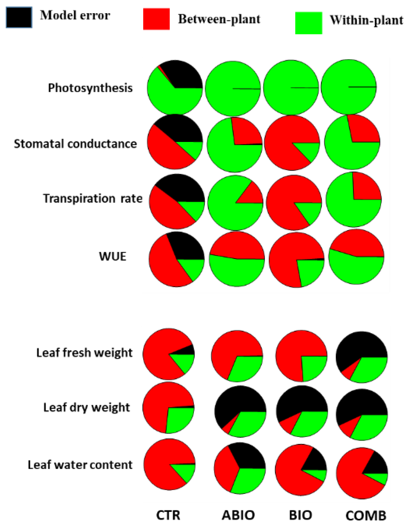
Within-Plant Variance of the Morpho-Physiological Traits
Morpho-Physiological Data
3. Results and Discussion
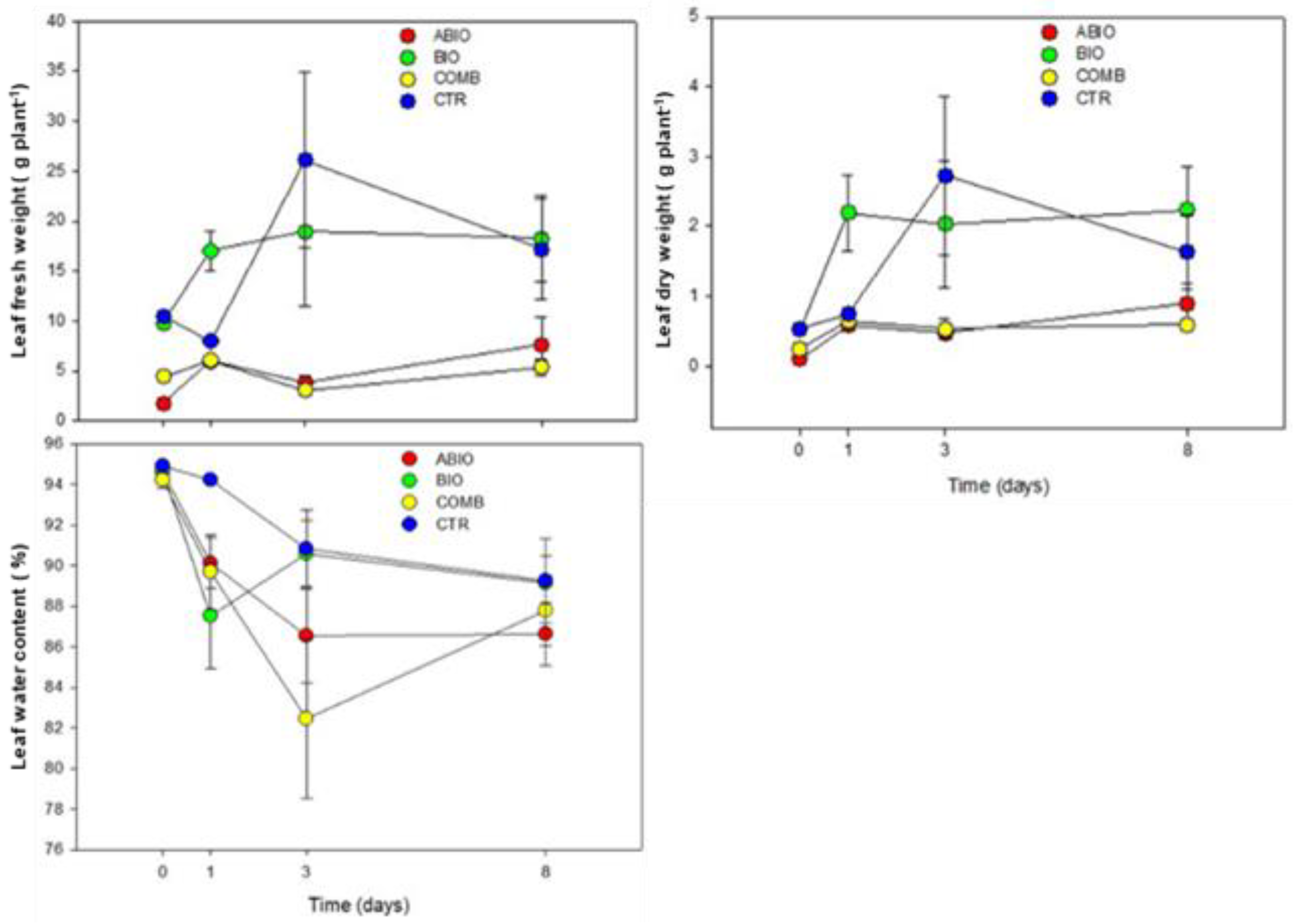
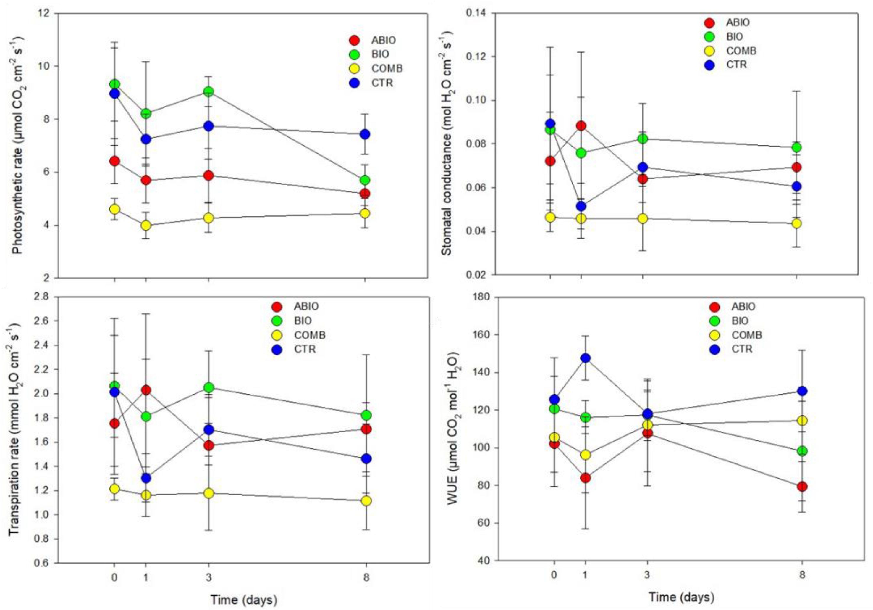
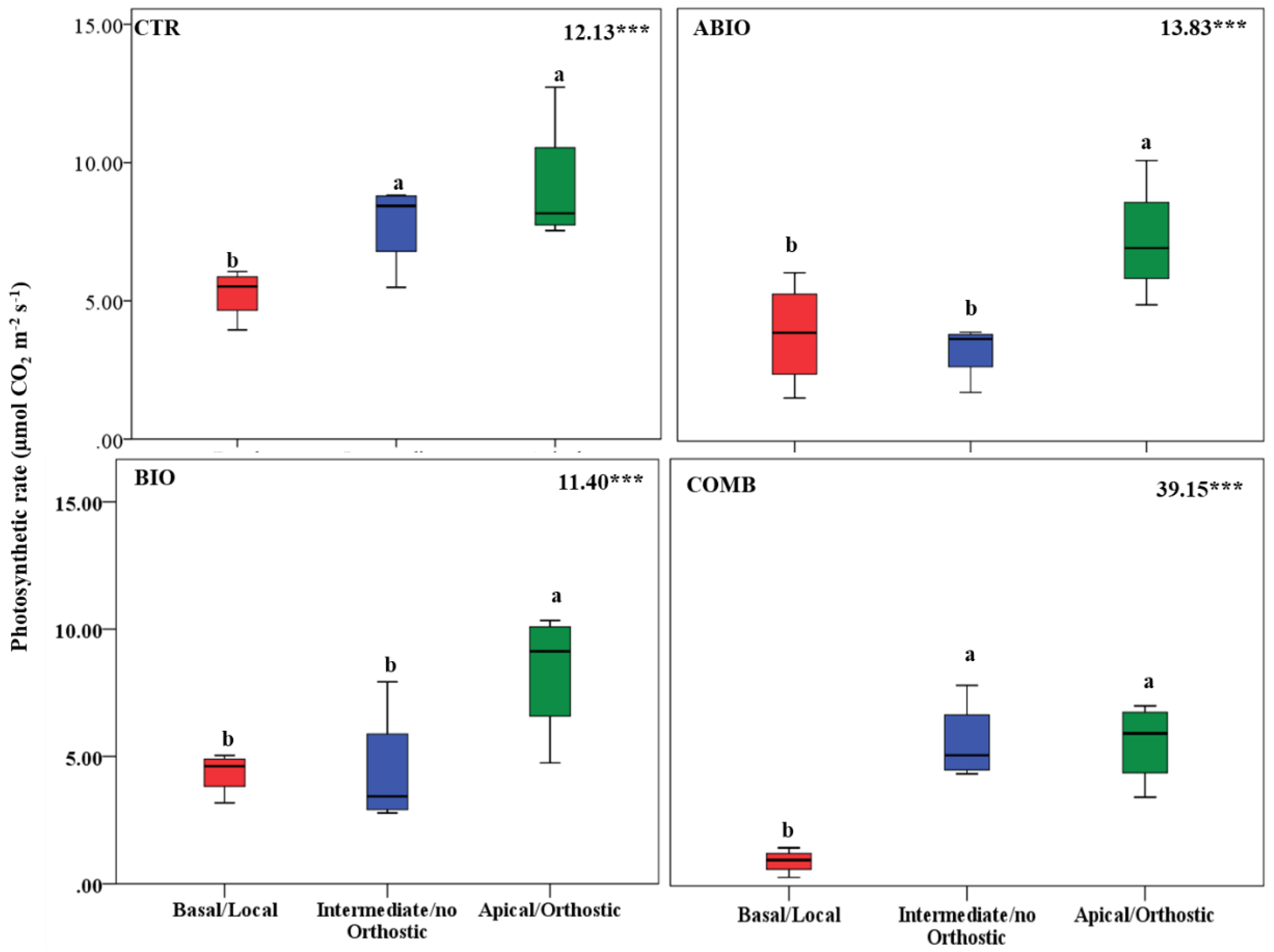
3.1. Are the Morpho-Physiological Responses to Individual Stresses Different from the Combined Ones? Are Additive, Synergistic or Antagonistic Effects in the Combined Stress?
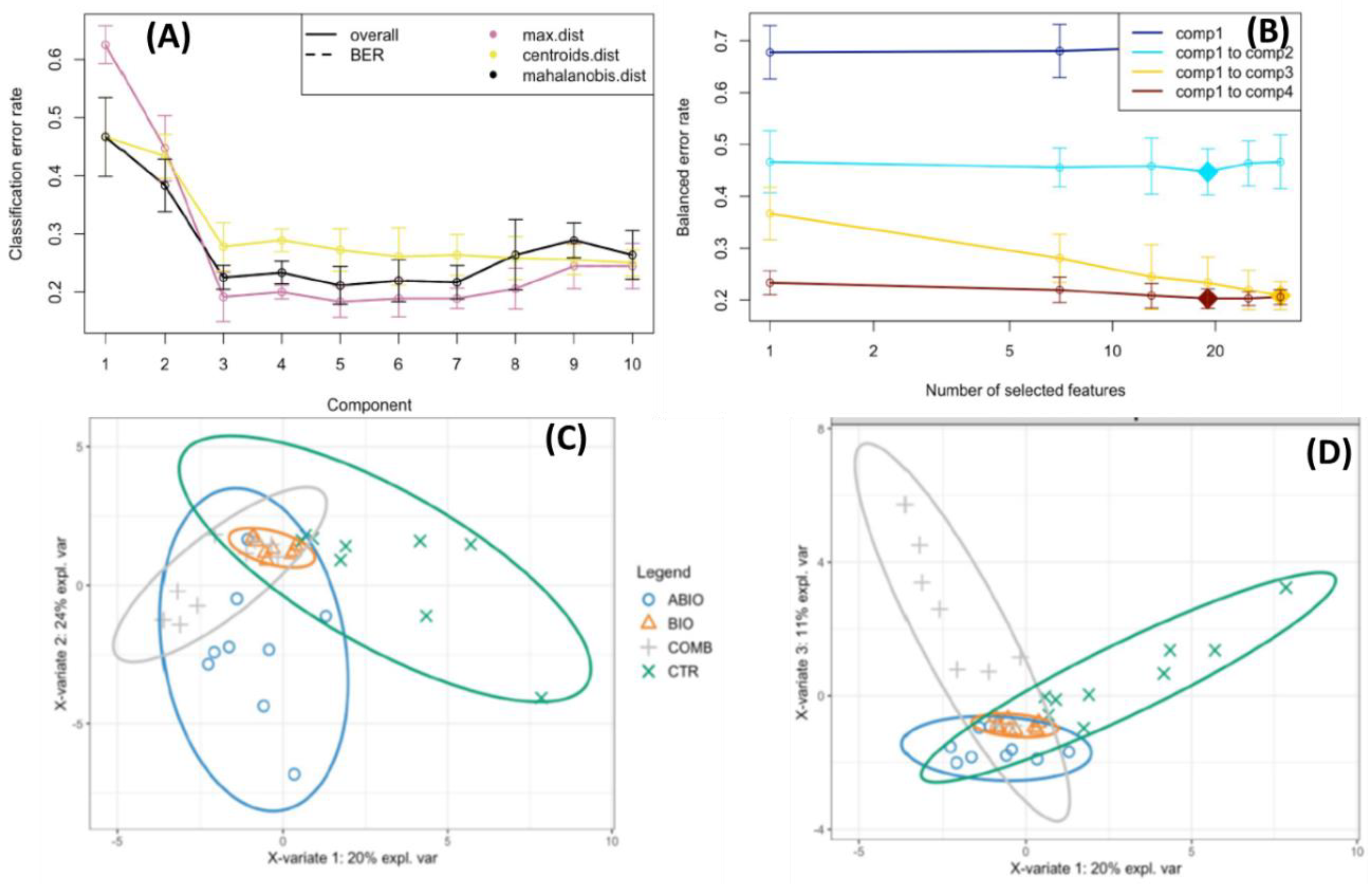
3.2. Are Additive, Synergistic or Antagonistic Effects in the Combined Stress?
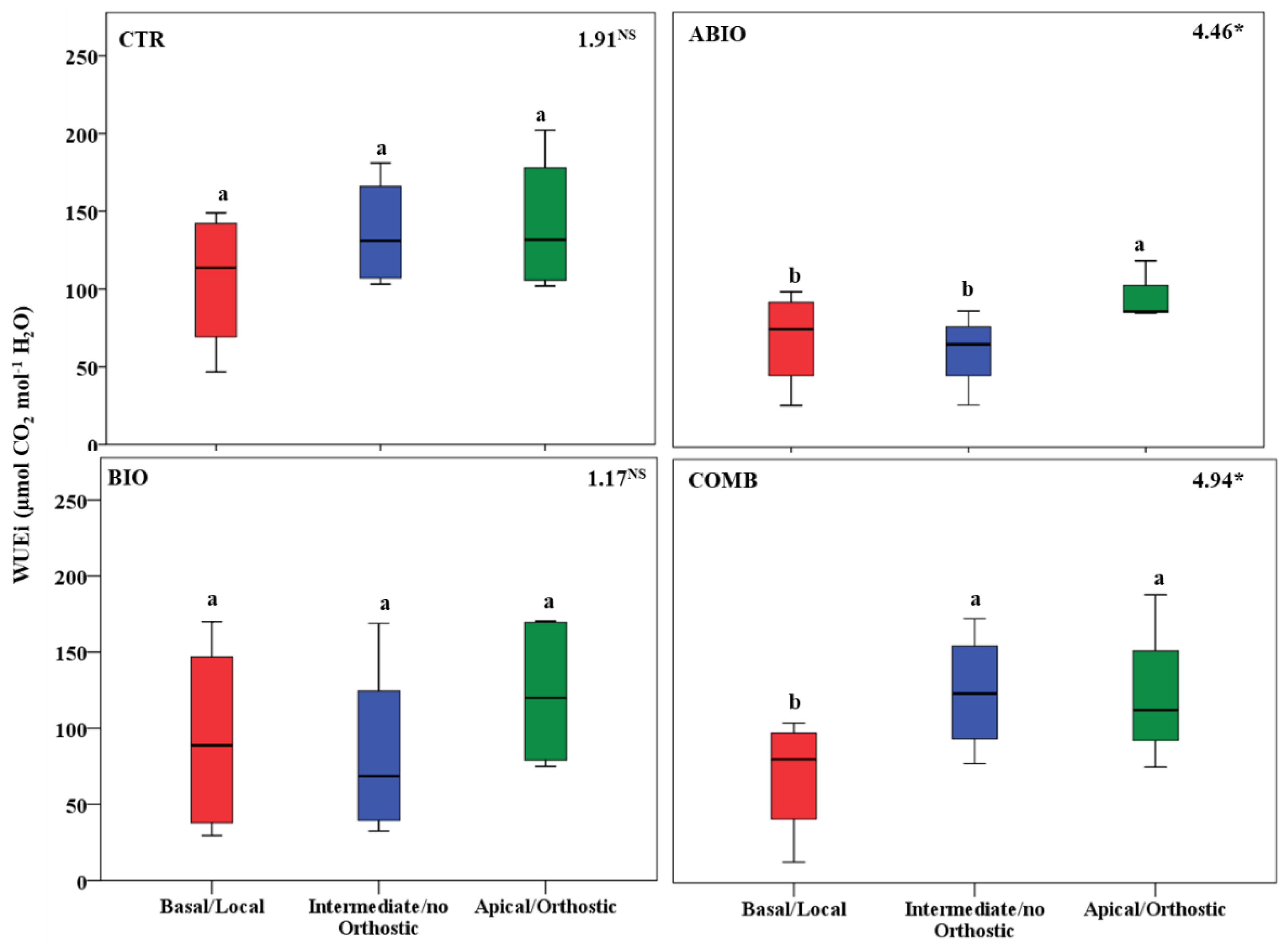
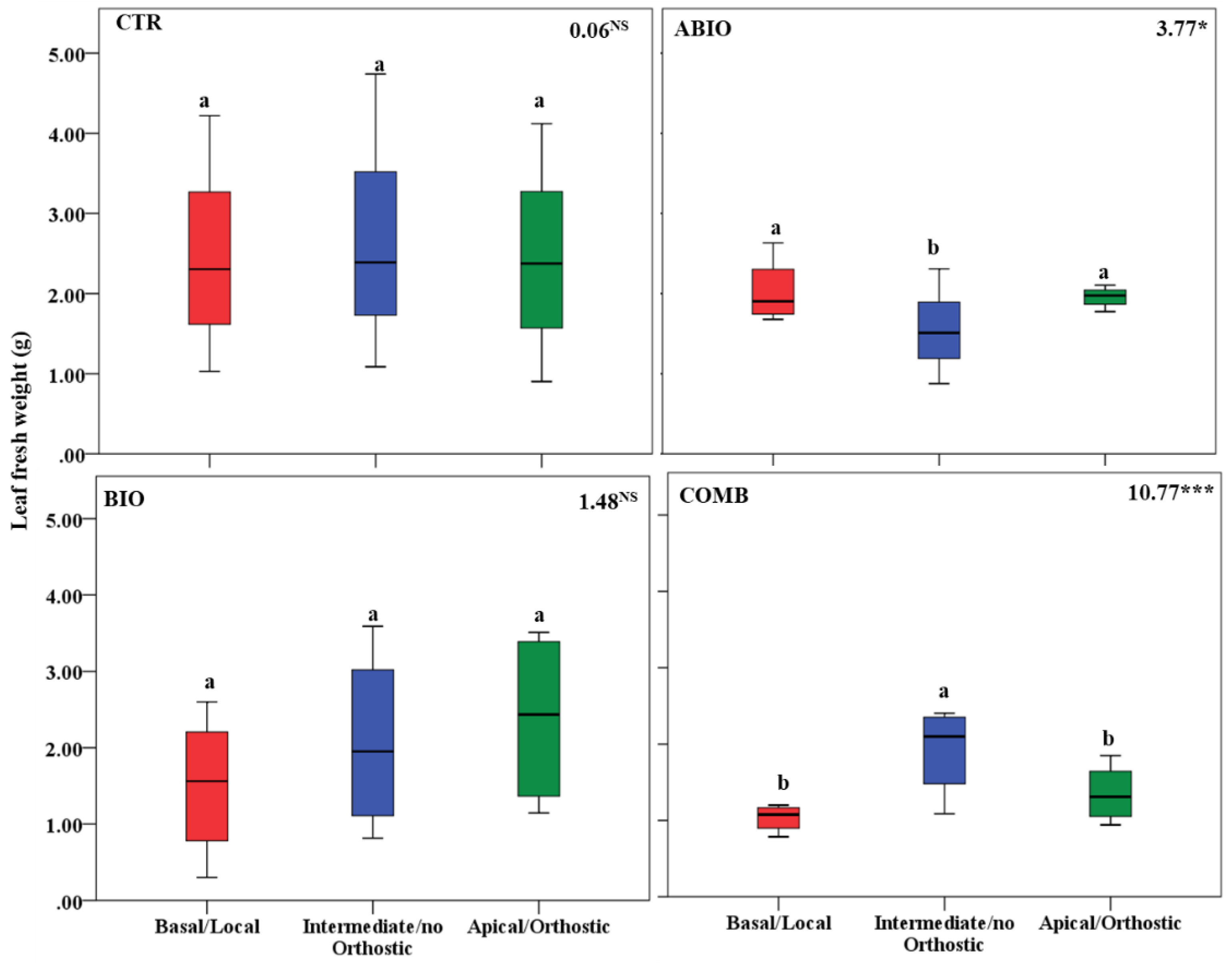
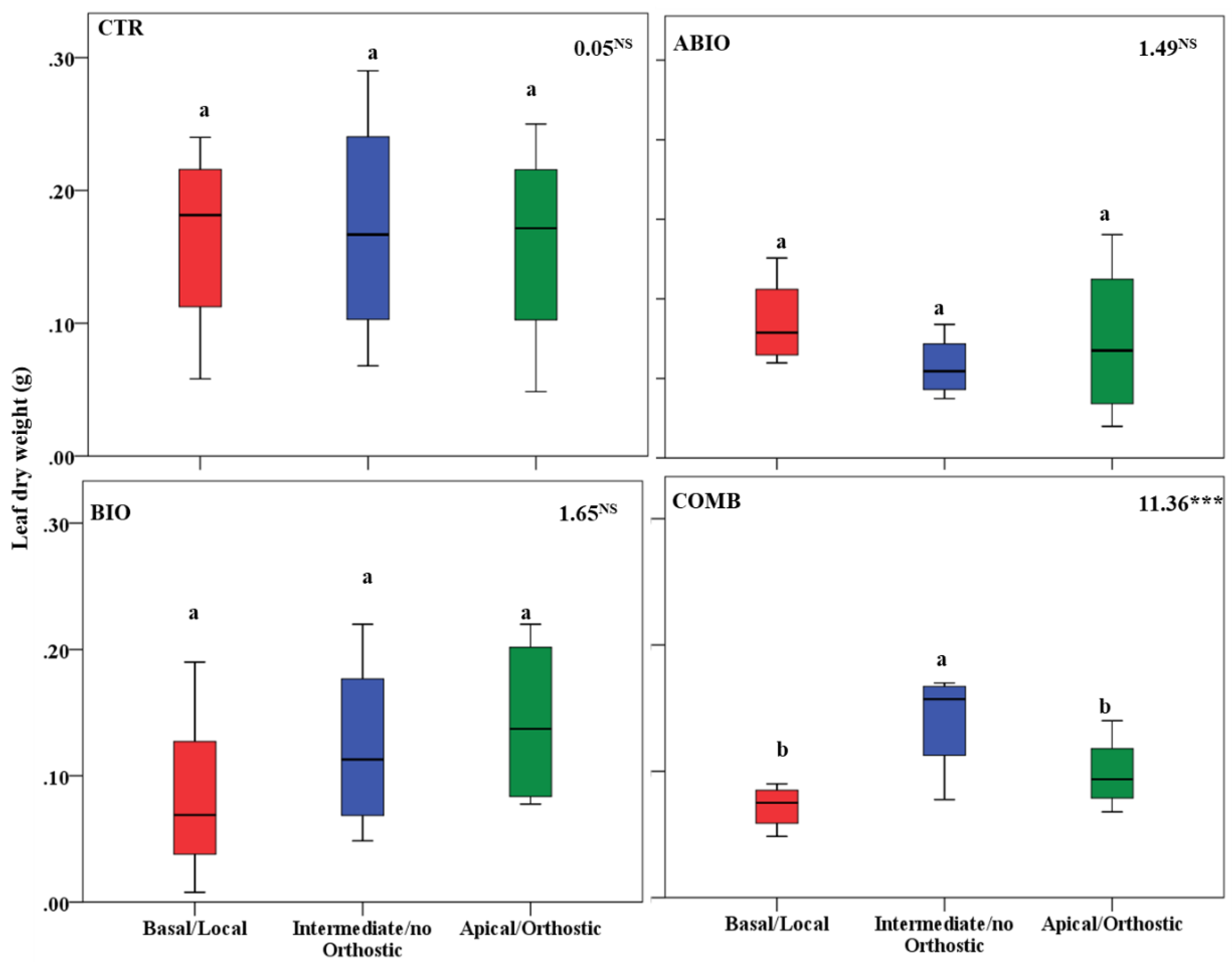
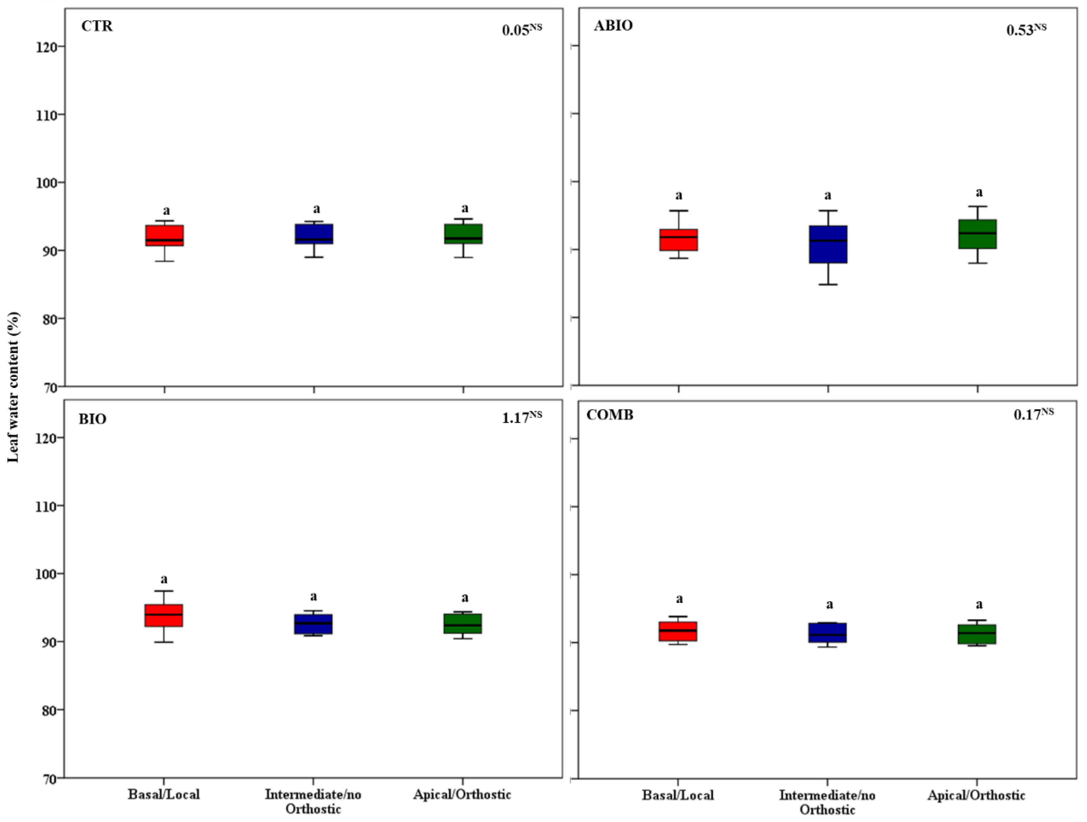
3.3. Do the Tomato Responses to the Single and Combined Stress Occur at Between- or Within-Plant Levels?
4. Conclusions and Future Directions
Supplementary Materials
Author Contributions
Funding
Institutional Review Board Statement
Informed Consent Statement
Data Availability Statement
Acknowledgments
Conflicts of Interest
References
- Heil, M.; Bostock, R.M. Induced systemic resistance (ISR) against pathogens in the context of induced plant defences. Ann. Bot. 2002, 89, 503–512. [Google Scholar] [CrossRef] [PubMed]
- He, M.; He, C.Q.; Ding, N.Z. Abiotic stresses: General defenses of land plants and chances for engineering multistress tolerance. Front. Plant Sci. 2018, 9, 1771. [Google Scholar] [CrossRef]
- Maron, J.L.; Cron, E. Herbivory: Effects on plant abundance, distribution and population growth. Proc. R. Soc. B 2006, 273, 2575–2584. [Google Scholar] [CrossRef]
- Mordecai, E.A. Pathogen impacts on plant communities: Unifying theory, concepts, and empirical work. Ecol. Monogr. 2011, 81, 429–441. [Google Scholar] [CrossRef]
- Pandey, P.; Irulappan, V.; Bagavathiannan, M.V.; Senthil-Kumar, M. Impact of combined abiotic and biotic stresses on plant growth and avenues for crop improvement by exploiting physio-morphological traits. Front. Plant Sci. 2017, 8, 537. [Google Scholar] [CrossRef]
- Vescio, R.; Abenavoli, M.R.; Sorgonà, A. Single and combined abiotic stress in maize root morphology. Plants 2021, 10, 5. [Google Scholar] [CrossRef]
- Vescio, R.; Malacrinò, A.; Bennett, A.E.; Sorgonà, A. Single and combined abiotic stressors affect maize rhizosphere bacterial microbiota. Rhizosphere 2021, 17, 100318. [Google Scholar] [CrossRef]
- Tiziani, R.; Miras-Moreno, B.; Malacrinò, A.; Vescio, R.; Lucini, L.; Mimmo, T.; Cesco, S.; Sorgonà, A. Drought, heat, and their combination impact the root exudation patterns and rhizosphere microbiome in maize roots. Environ. Exp. Bot. 2022, 203, 105071. [Google Scholar] [CrossRef]
- Havko, N.E.; Das, M.R.; McClain, A.M.; Kapali, G.; Sharkey, T.D.; Howe, G.A. Insect herbivory antagonizes leaf cooling responses to elevated temperature in tomato. Proc. Nat. Acad. Sci. USA 2020, 117, 2211–2217. [Google Scholar] [CrossRef]
- Catola, S.; Centritto, M.; Cascone, P.; Ranieri, A.; Loreto, F.; Calamai, L.; Balestrini, R.; Guerrieri, E. Effects of single or combined water deficit and aphid attack on tomato volatile organic compound (VOC) emission and plant-plant communication. Environ. Exp. Bot. 2018, 153, 54–62. [Google Scholar] [CrossRef]
- Copolovici, L.; Kännaste, A.; Remmel, T.; Niinemets, Ü. Volatile organic compound emissions from Alnus glutinosa under interacting drought and herbivory stresses. Environ. Exp. Bot. 2014, 100, 55–63. [Google Scholar] [CrossRef] [PubMed]
- Bansal, S.; Hallsby, G.; Löfvenius, M.O.; Nilsson, M.C. Synergistic, additive and antagonistic impacts of drought and herbivory on Pinus sylvestris: Leaf, tissue and whole-plant responses and recovery. Tree Physiol. 2013, 33, 451–463. [Google Scholar] [CrossRef] [PubMed]
- Mason, C.J.; Villari, C.; Keefover-Ring, K.; Jagemann, S.; Zhu, J.; Bonello, P.; Raffa, K.F. Spatial and temporal components of induced plant responses in the context of herbivore life history and impact on host. Funct. Ecol. 2017, 31, 2034–2050. [Google Scholar] [CrossRef]
- Orians, C.M. Herbivores, vascular pathways, and systemic induction: Facts and artifacts. J. Chem. Ecol. 2005, 31, 2231–2242. [Google Scholar] [CrossRef] [PubMed]
- Park, S.W.; Kaimoyo, E.; Kumar, D.; Mosher, S.; Klessig, D.F. Methyl salicylate is a critical mobile signal for plant systemic acquired resistance. Science 2007, 318, 113–116. [Google Scholar] [CrossRef] [PubMed]
- Slot, M.; Krause, G.H.; Krause, B.; Hernández, G.G.; Winter, K. Photosynthetic heat tolerance of shade and sun leaves of three tropical tree species. Photosynth. Res. 2019, 141, 119–130. [Google Scholar] [CrossRef]
- Rubio, G.; Sorgonà, A.; Lynch, J.P. Spatial mapping of phosphorus influx in bean root systems using digital autoradiography. J. Exp. Bot. 2004, 55, 2269–2280. [Google Scholar] [CrossRef]
- Sorgonà, A.; Abenavoli, M.R.; Gringeri, P.G.; Cacco, G. Comparing morphological plasticity of root orders in slow- and fast-growing citrus rootstocks supplied with different nitrate levels. Ann. Bot. 2007, 100, 1287–1296. [Google Scholar] [CrossRef]
- Boege and Marquis Facing herbivory as you grow up: The ontogeny of resistance in plants. Trends Ecol. Evol. 2005, 20, 441–444. [CrossRef]
- Holeski, L.M. Within and between generation phenotypic plasticity in trichome density of Mimulus guttatus. J. Evol. Biol. 2007, 20, 2092–2100. [Google Scholar] [CrossRef]
- Kollist, H.; Zandalinas, S.I.; Sengupta, S.; Nuhkat, M.; Kangasjärvi, J.; Mittler, R. Rapid responses to abiotic stress: Priming the landscape for the signal transduction network. Trends Plant Sci. 2019, 24, 25–37. [Google Scholar] [CrossRef] [PubMed]
- Hidalgo, J.; Rubio de Casas, R.; Muñoz, M.A. Environmental unpredictability and inbreeding depression select for mixed dispersal syndromes. BMC Evol. Biol. 2016, 16, 71. [Google Scholar] [CrossRef] [PubMed]
- Wetzel, W.C.; Meek, M.H. Physical defenses and herbivory vary more within plants than among plants in the tropical understory shrub Piper polytrichum. Botany 2019, 97, 113–121. [Google Scholar] [CrossRef]
- Herrera, C.M.; Medrano, M.; Bazaga, P. Continuous within plant variation as a source of intraspecific functional diversity: Patterns, magnitude, and genetic correlates of leaf variability in Helleborus foetidus (Ranunculaceae). Am. J. Bot. 2015, 102, 225–232. [Google Scholar] [CrossRef] [PubMed]
- Desneux, N.; Luna, M.G.; Guillemaud, T.; Urbaneja, A. The invasive South American tomato pinworm, Tuta absoluta, continues to spread in Afro-Eurasia and beyond—The new threat to tomato world production. J. Pest Sci. 2011, 84, 403–408. [Google Scholar] [CrossRef]
- Han, P.; Lavoir, A.V.; Le Bot, J.; Amiens-Desneux, E.; Desneux, N. Nitrogen and water availability to tomato plants triggers bottom-up effects on the leafminer Tuta absoluta. Sci. Rep. 2014, 4, 4455. [Google Scholar] [CrossRef]
- Larbat, R.; Adamowicz, S.; Robin, C.; Han, P.; Desneux, N.; Le Bot, J. Interrelated responses of tomato plants and the leaf miner Tuta absoluta to nitrogen supply. Plant Biol. 2016, 18, 495–504. [Google Scholar] [CrossRef]
- Ahmed, I.M.; Dai, H.; Zheng, W.; Cao, F.; Zhang, G.; Sun, D.; Wu, F. Genotypic differences in physiological characteristics in the tolerance to drought and salinity combined stress between Tibetan wild and cultivated barley. Plant Physiol. Biochem. 2013, 63, 49–60. [Google Scholar] [CrossRef]
- Schädler, M.; Jung, G.; Auge, H.; Brandl, R. Palatability, decomposition and insect herbivory: Patterns in a successional old-field plant community. Oikos 2003, 103, 121–132. [Google Scholar] [CrossRef]
- Flexas, J.; Carriquí, M.; Nadal, M. Gas exchange and hydraulics during drought in crops: Who drives whom? J. Exp. Bot. 2018, 69, 3791–3795. [Google Scholar] [CrossRef]
- Schwarz, D.; Kläring, H.P.; van Iersel, M.W.; Ingram, K.T. Growth and Photosynthetic response of tomato to nutrient solution concentration at two light levels. J. Am. Soc. Hort. Sci. 2002, 127, 984–990. [Google Scholar] [CrossRef]
- Kerchev, P.I.; Fenton, B.; Foyer, C.H.; Hancock, R.D. Plant responses to insect herbivory: Interactions between photosynthesis, reactive oxygen species and hormonal signalling pathways. Plant Cell Environ. 2012, 35, 441–453. [Google Scholar] [CrossRef] [PubMed]
- Holopainen, J.K.; Gershenzon, J. Multiple stress factors and the emission of plant VOCs. Trends Plant Sci. 2010, 15, 176–184. [Google Scholar] [CrossRef] [PubMed]
- IPCC. Climate Change and Land: An IPCC Special Report on Climate Change, Desertification, Land Degradation, Sustainable Land Management, Food Security, and Greenhouse Gas Fluxes in Terrestrial Ecosystems; IPCC: Geneva, Switzerland, 2019. [Google Scholar]
- Seibt, U.; Rajabi, A.; Griffiths, H.; Berry, J.A. Carbon isotopes and water use efficiency: Sense and sensitivity. Oecologia 2008, 155, 441–454. [Google Scholar] [CrossRef]
- Jin, X.; Shi, C.; Yu, C.Y.; Yamada, T.; Sacks, E.J. Determination of leaf water content by visible and near-infrared spectrometry and multivariate calibration in Miscanthus. Front. Plant Sci. 2017, 8, 721. [Google Scholar] [CrossRef] [PubMed]
- Van den Dool, H.; Kratz, P.D. A generalization of the retention index system including linear temperature programmed gas-liquid partition chromatography. J. Chromatogr. 1963, 11, 463–471. [Google Scholar] [CrossRef]
- R Core Team. R: A Language and Environment for Statistical Computing; R Foundation for Statistical Computing: Vienna, Austria, 2020; Available online: https://www.R-project.org/ (accessed on 3 June 2020).
- Rohart, F.; Gautier, B.; Singh, A.; Lê Cao, K.A. mixOmics: An R package for ‘omics feature selection and multiple data integration. PLoS Comput. Biol. 2017, 13, e1005752. [Google Scholar] [CrossRef]
- Darling, E.S.; McClanahan, T.R.; Côté, I.M. Combined effects of two stressors on Kenyan coral reefs are additive or antagonistic, not synergistic. Conserv. Lett. 2010, 3, 122–130. [Google Scholar] [CrossRef]
- Orians, C.M.; Pomerleau, J.; Ricco, R. Vascular architecture generates fine scale variation in the systemic induction of proteinase inhibitors in tomato. J. Chem. Ecol. 2000, 26, 471–485. [Google Scholar] [CrossRef]
- Zywiec, M.; Delibes, M.; Fedriani, J.M. Microgeographical, interindividual, and intra-individual variation in the flower characters of Iberian pear Pyrus bourgaeana (Rosaceae). Oecologia 2012, 169, 713–722. [Google Scholar] [CrossRef]
- Liang, G.; Liu, J.; Zhang, J.; Guo, J. Effects of drought stress on photosynthetic and physiological parameters of tomato. J. Am. Soc. Hort. Sci. 2020, 145, 12–17. [Google Scholar] [CrossRef]
- García, A.L.; Marcelis, L.; Garcia-Sanchez, F.; Nicolas, N.; Martínez, V. Moderate water stress affects tomato leaf water relations in dependence on the nitrogen supply. Biol. Plant. 2007, 51, 707–712. [Google Scholar] [CrossRef]
- Tamburino, R.; Vitale, M.; Ruggiero, A.; Sassi, M.; Sannino, L.; Arena, S.; Grillo, S. Chloroplast proteome response to drought stress and recovery in tomato (Solanum lycopersicum L.). BMC Plant Biol. 2017, 17, 40. [Google Scholar] [CrossRef] [PubMed]
- Grinnan, R.; Carter, T.E.; Johnson, M.T.J. The effects of drought and herbivory on plant–herbivore interactions across 16 soybean genotypes in a field experiment. Ecol. Entomol. 2013, 38, 290–302. [Google Scholar] [CrossRef]
- Zangerl, A.R.; Hamilton, J.G.; Miller, T.J.; Crofts, A.R.; Oxborough, K.; Berenbaum, M.R.; DeLucia, E.H. Impact of folivory on photosynthesis is greater than the sum of its holes. Proc. Nat. Acad. Sci. USA 2002, 99, 1088–1091. [Google Scholar] [CrossRef]
- Thomson, V.P.; Cunningham, S.A.; Ball, M.C.; Nicotra, A.B. Compensation for herbivory by Cucumis sativus through increased photosynthetic capacity and efficiency. Oecologia 2003, 134, 167–175. [Google Scholar] [CrossRef]
- Aldea, M.; Hamilton, J.G.; Resti, J.P.; Zangerl, A.R.; Berenbaum, M.R.; Delucia, E.H. Indirect effects of insect herbivory on leafgas exchange in soybean. Plant Cell Environ. 2005, 28, 402–411. [Google Scholar] [CrossRef]
- Coqueret, V.; Le Bot, J.; Larbat, R.; Desneux, N.; Robin, C.; Adamowicz, S. Nitrogen nutrition of tomato plant alters leafminer dietary intake dynamics. J. Insect Physiol. 2017, 99, 130–138. [Google Scholar] [CrossRef]
- Nguyen, D.; Poeschl, Y.; Lortzing, T.; Hoogveld, R.; Gogol-Döring, A.; Cristescu, S.M.; Steppuhn, A.; Mariani, C.; Rieu, I.; van Dam, N.M. Interactive responses of Solanum dulcamara to drought and insect feeding are herbivore species-specific. Int. J. Mol. Sci. 2018, 19, 3845. [Google Scholar] [CrossRef]
- Mou, P.; Jones, R.H.; Tan, Z.; Bao, Z.; Chen, H. Morphological and physiological plasticity of plant roots when nutrients are both spatially and temporally heterogeneous. Plant Soil 2013, 364, 373–384. [Google Scholar] [CrossRef]
- Puglielli, G.; Catoni, R.; Spoletini, A.; Varone, L.; Gratani, L. Short-term physiological plasticity: Trade-off between drought and recovery responses in three Mediterranean Cistus species. Ecol. Evol. 2017, 7, 10880–10889. [Google Scholar] [CrossRef]
- Wagner, M.R.; Mitchell-Olds, T. Plasticity of plant defense and its evolutionary implications in wild populations of Boechera stricta. Evolution 2018, 72, 1034–1049. [Google Scholar] [CrossRef] [PubMed]
- Foti, V.; Araniti, F.; Manti, F.; Alicandri, E.; Giuffrè, A.M.; Bonsignore, C.P.; Castiglione, E.; Sorgonà, A.; Covino, S.; Paolacci, A.R.; et al. Profiling volatile terpenoids from Calabrian Pine stands infested by the Pine processionary Moth. Plants 2020, 9, 1362. [Google Scholar] [CrossRef] [PubMed]
- Loreto, F.; Schnitzler, P. Abiotic stresses and induced BVOCs. Trends Plant Sci. 2010, 15, 154–166. [Google Scholar] [CrossRef] [PubMed]
- Tholl, D. Biosynthesis and biological functions of terpenoids in plants. In Biotechnology of Isoprenoids; Springer: Cham, Switzerland, 2015; Volume 148, pp. 63–106. [Google Scholar]
- Silva, D.B.; Weldegergis, B.T.; Van Loon, J.J.; Bueno, V.H. Qualitative and quantitative differences in herbivore-induced plant volatile blends from tomato plants infested by either Tuta absoluta or Bemisia tabaci. J. Chem. Ecol. 2017, 43, 53–65. [Google Scholar] [CrossRef] [PubMed]
- Deglow, E.; Borden, J. Green leaf volatiles disrupt and enhance response to aggregation pheromones by the ambrosia beetle, Gnathotrichus sulcatus (Coleoptera: Scolytidae). Can. J. For. Res. 2011, 28, 1697–1705. [Google Scholar] [CrossRef]
- Ruther, J. Retention index database for identification of general green leaf volatiles in plants by coupled capillary gas chromatography−mass spectrometry. J. Chromatogr. 2000, 890, 313–319. [Google Scholar] [CrossRef]
- Rodriguez-Saona, C.; Parra, L.; Quiroz, A.; Isaacs, R. Variation in highbush blueberry floral volatile profiles as a function of pollination status, cultivar, time of day and flower part: Implications for flower visitation by bees. Ann. Bot. 2011, 107, 1377–1390. [Google Scholar] [CrossRef]
- Muhammad, H.; Zamri, Z.; Ismanizan, I. Green leaf volatiles: Biosynthesis, biological functions and their applications in biotechnology. Plant Biotechnol. J. 2015, 13, 727–739. [Google Scholar]
- Mayo-Hernández, J.; Ramírez-Chávez, E.; Molina-Torres, J.; Guillén-Cisneros, M.L.; Rodríguez-Herrera, R.; Hernández-Castillo, F.; Flores-Olivas, A.; Valenzuela Soto, J.H. Effects of Bactericera cockerelli herbivory on volatile emissions of three varieties of Solanum lycopersicum. Plants 2019, 8, 509. [Google Scholar] [CrossRef]
- López, Y.I.Á.; Martínez-Gallardo, N.A.; Ramírez-Romero, R.; López, M.G.; Sánchez-Hernández, C.; Délano-Frier, J.P. Cross-kingdom effects of plant plant signaling via volatile organic compounds emitted by tomato (Solanum lycopersicum) plants infested by the greenhouse whitefly (Trialeurodes vaporariorum). J. Chem. Ecol. 2012, 38, 1376–1386. [Google Scholar] [CrossRef]
- Islam, M.N.; Hasanuzzaman, A.T.M.; Zhang, Z.F.; Zhang, Y.; Liu, T.X. High level of nitrogen makes tomato plants releasing less volatiles and attracting more Bemisia tabaci (Hemiptera: Aleyrodidae). Front. Plant Sci. 2017, 8, 466. [Google Scholar] [CrossRef] [PubMed]
- Giunti, G.; Benelli, G.; Conte, G.; Mele, M.; Caruso, G.; Gucci, R.; Flamini, G.; Canale, A. VOCs-mediated location of olive fly larvae by the braconid parasitoid Psyttalia concolor: A multivariate comparison among VOC bouquets from three olive cultivars. BioMed Res. Int. 2016, 2016, 7827615. [Google Scholar] [CrossRef] [PubMed]
- Mahdavi, A.; Moradi, P.; Mastinu, A. Variation in terpene profiles of Thymus vulgaris in water deficit stress response. Molecules 2020, 25, 1091. [Google Scholar] [CrossRef] [PubMed]
- Tan, X.P.; Liang, W.Q.; Liu, C.J.; Luo, P.; Heinstein, P.; Chen, X.Y. Expression pattern of (+)-delta-cadinene synthase genes and biosynthesis of sesquiterpene aldehydes in plants of Gossypium arboreum L. Planta 2000, 210, 644–651. [Google Scholar] [CrossRef]
- Errard, A.; Ulrichs, C.; Kühne, S.; Mewis, I.; Drungowski, M.; Schreiner, M.; Baldermann, S. Single- versus multiple-pest infestation affects differently the biochemistry of tomato (Solanum lycopersicum ‘Ailsa Craig’). J. Agric. Food Chem. 2015, 63, 10103–10111. [Google Scholar] [CrossRef] [PubMed]
- Weldegergis, B.T.; Zhu, F.; Poelman, E.H.; Dicke, M. Drought stress affects plant metabolites and herbivore preference but not host location by its parasitoids. Oecologia 2015, 177, 701–713. [Google Scholar] [CrossRef]
- Takahashi, F.; Kuromori, T.; Urano, K.; Yamaguchi-Shinozaki, K.; Shinozaki, K. Drought stress responses and resistance in plants: From cellular responses to long-distance intercellular communication. Front. Plant Sci. 2020, 11, 556972. [Google Scholar] [CrossRef]
- Nguyen, D.; Rieu, I.; Mariani, C.; van Dam, N.M. How plants handle multiple stresses: Hormonal interactions underlying responses to abiotic stress and insect herbivory. Plant Mol. Biol. 2016, 91, 727–740. [Google Scholar] [CrossRef] [PubMed]
- Yang, J.; Duan, G.; Li, C.; Liu, L.; Han, G.; Zhang, Y.; Wang, C. The crosstalks between jasmonic acid and other plant hormone signaling highlight the involvement of Jasmonic Acid as a core component inplant response to biotic and abiotic stresses. Front. Plant Sci. 2019, 10, 1349. [Google Scholar] [CrossRef]
- Hossain, M.A.; Munemasa, S.; Uraji, M.; Nakamura, Y.; Mori Izumi, C.; Murata, Y. Involvement of endogenous abscisic acid in Methyl Jasmonate-induced stomatal closure in Arabidopsis. Plant Physiol. 2011, 156, 430–438. [Google Scholar] [CrossRef]
- Atkinson, N.J.; Lilley, C.J.; Urwin, P.E. Identification of genes involved in the response of Arabidopsis to simultaneous biotic and abiotic stresses. Plant Physiol. 2013, 162, 2028–2041. [Google Scholar] [CrossRef] [PubMed]
- Prasch, C.M.; Sonnewald, U. Simultaneous application of heat, drought, and virus to Arabidopsis plants reveals significant shifts in signaling networks. Plant Physiol. 2013, 162, 1849–1866. [Google Scholar] [CrossRef] [PubMed]
- Coolen, S.; Proietti, S.; Hickman, R.; Davila Olivas, N.H.; Huang, P.P.; Van Verk, M.C.; Van Pelt, J.A.; Wittenberg, A.H.; De Vos, M.; Prins, M.; et al. Transcriptome dynamics of Arabidopsis during sequential biotic and abiotic stresses. Plant J. 2016, 86, 249–267. [Google Scholar] [CrossRef]
- Nabity, P.D.; Zavala, J.A.; DeLucia, E.H. Indirect suppression of photosynthesis on individual leaves by arthropod herbivory. Ann. Bot. 2009, 103, 655–663. [Google Scholar] [CrossRef] [PubMed]
- Schmidt, L.; Schurr, U.; Röse, U.S.R. Local and systemic effects of two herbivores with different feeding mechanisms on primary metabolism of cotton leaves. Plant Cell Environ. 2009, 32, 893–903. [Google Scholar] [CrossRef] [PubMed]
- Chaves, M.M.; Flexas, J.; Pinheiro, C. Photosynthesis under drought and salt stress: Regulation mechanisms from whole plant to cell. Ann. Bot. 2009, 103, 551–560. [Google Scholar] [CrossRef] [PubMed]
- Shin, R.; Berg, R.H.; Schachtman, D.P. Reactive oxygen species and root hairs in Arabidopsis root response to nitrogen, phosphorus and potassium deficiency. Plant Cell Physiol. 2005, 46, 1350–1357. [Google Scholar] [CrossRef]
- Arimura, G.I.; Ozawa, R.; Maffei, M.E. Recent advances in plant early signaling in response to herbivory. Int. J. Mol. Sci. 2011, 12, 3723–3739. [Google Scholar] [CrossRef]
- Thompson, G.A.; Goggin, F.L. Transcriptomics and functional genomics of plant defence induction by phloem-feeding insects. J. Exp. Bot. 2006, 57, 755–766. [Google Scholar] [CrossRef]
- Elger, A.; Willby, N.J. Leaf dry matter content as an integrative expression of plant palatability: The case of freshwater macrophytes. Funct. Ecol. 2003, 17, 58–65. [Google Scholar] [CrossRef]
- Grime, J.P.; Cornelissen, J.H.C.; Thompson, K.; Hodgson, J.G. Evidence of a causal connection between antiherbivore defence and the decomposition rate of leaves. Oikos 1996, 77, 489–494. [Google Scholar] [CrossRef]
- Herrera, C.M. Multiplicity in Unity: Plant Subindividual Variation and Interactions with Animals; University of Chicago Press: Chicago, IL, USA, 2009. [Google Scholar]
- Herrera, C.M. The ecology of subindividual variability in plants: Patterns, processes, and prospects. Web Ecol. 2017, 17, 51–64. [Google Scholar] [CrossRef]
- Osada, N.; Yasumura, Y.; Ishida, A. Leaf nitrogen distribution in relation to crown architecture in the tall canopy species, Fagus crenata. Oecologia 2014, 175, 1093–1106. [Google Scholar] [CrossRef]
- Meldau, S.; Erb, M.; Baldwin, I.T. Defence on demand: Mechanisms behind optimal defence patterns. Ann. Bot. 2012, 110, 1503–1514. [Google Scholar] [CrossRef] [PubMed]
- Devireddy, A.R.; Zandalinas, S.I.; Gómez-Cadenas, A.; Blumwald, E.; Mittler, R. Coordinating the overall stomatal response of plants: Rapid leaf-to-leaf communication during light stress. Sci. Signal. 2018, 11, 518. [Google Scholar] [CrossRef]
- Girón-Calva, P.S.; Li, T.; Koski, T.M.; Klemola, T.; Laaksonen, T.; Huttunen, L.; Blande, J.D. A role for volatiles in intra- and inter-plant interactions in birch. J. Chem. Ecol. 2014, 40, 1203–1211. [Google Scholar] [CrossRef]
- Meier, I.C.; Leuschner, C. Genotypic variation and phenotypic plasticity in the drought response of fine roots of European beech. Tree Physiol. 2008, 28, 297–309. [Google Scholar] [CrossRef]
- Rodriguez-Saona, C.R.; Rodriguez-Saona, L.E.; Frost, C.J. Herbivore induced volatiles in the perennial shrub, Vaccinium corymbosum, and their role in inter-branch signaling. J. Chem. Ecol. 2009, 35, 163–175. [Google Scholar] [CrossRef] [PubMed]
- Schurr, U.; Walter, A.; Rascher, U. Functional dynamics of plant growth and photosynthesis–from steady-state to dynamics–from homogeneity to heterogeneity. Plant Cell Environ. 2006, 29, 340–352. [Google Scholar] [CrossRef]
- Berens, M.L.; Wolinska, K.W.; Spaepen, S.; Ziegler, J.; Nobori, T.; Nair, A.; Krüler, V.; Winkelmüller, T.M.; Wang, Y.; Mine, A.; et al. Balancing trade-offs between biotic and abiotic stress responses through leaf age-dependent variation in stress hormone cross-talk. Proc. Nat. Acad. Sci. USA 2019, 116, 2364–2373. [Google Scholar] [CrossRef] [PubMed]


| Parameters | Statistics | Time (Ti) | ||||
|---|---|---|---|---|---|---|
| Treatments (Tr) | t0 | t1 | t3 | t8 | ||
| Leaf fresh weight | Tr 10.92 *** | ABIO | a | a | b | b |
| Ti 1.40 NS | BIO | a | a | a | a | |
| Bl 6.08 * | COMB | a | a | b | b | |
| TrxTi 1.06 NS | CTR | a | a | a | a | |
| Leaf dry weight | Tr 8.87 *** | ABIO | a | a | b | b |
| Ti 2.91 * | BIO | a | a | a | a | |
| BI 17.17 *** | COMB | a | a | b | b | |
| TrxTi 1.26 NS | CTR | a | a | a | ab | |
| Leaf water content | Tr 3.16 * | ABIO | a | ab | ab | a |
| Ti 12.01 *** | BIO | a | b | a | a | |
| BI 52.15 *** | COMB | a | b | b | a | |
| TrxTi 1.50 NS | CTR | a | a | a | a | |
| Parameters | Statistics | Time (Ti) | ||||
|---|---|---|---|---|---|---|
| Treatments (Tr) | t0 | t1 | t3 | t8 | ||
| Photosynthetic rate | Tr 17.60 *** | ABIO | a | b | bc | ab |
| Ti 2.73 NS | BIO | a | a | a | ab | |
| BI 20.74 *** | COMB | a | b | c | b | |
| TrxTi 0.76 NS | CTR | a | ab | ab | a | |
| Stomatal conductance | Tr 5.38 ** | ABIO | a | a | ab | a |
| Ti 0.60 NS | BIO | a | a | a | a | |
| BI 61.82 *** | COMB | a | b | b | a | |
| TrxTi 0.57 NS | CTR | a | ab | ab | a | |
| Transpiration rate | Tr 6.94 ** | ABIO | a | a | ab | ab |
| Ti 0.79 NS | BIO | a | a | a | a | |
| BI 55.73 *** | COMB | a | a | b | b | |
| TrxTi 1.13 NS | CTR | a | a | ab | ab | |
| iWUE | Tr 6.23 ** | ABIO | a | b | a | b |
| Ti 0.47 NS | BIO | a | b | a | b | |
| BI 136.54 *** | COMB | a | b | a | ab | |
| TrxTi 1.52 NS | CTR | a | a | a | a | |
Publisher’s Note: MDPI stays neutral with regard to jurisdictional claims in published maps and institutional affiliations. |
© 2022 by the authors. Licensee MDPI, Basel, Switzerland. This article is an open access article distributed under the terms and conditions of the Creative Commons Attribution (CC BY) license (https://creativecommons.org/licenses/by/4.0/).
Share and Cite
Vescio, R.; Caridi, R.; Laudani, F.; Palmeri, V.; Zappalà, L.; Badiani, M.; Sorgonà, A. Abiotic and Herbivory Combined Stress in Tomato: Additive, Synergic and Antagonistic Effects and Within-Plant Phenotypic Plasticity. Life 2022, 12, 1804. https://doi.org/10.3390/life12111804
Vescio R, Caridi R, Laudani F, Palmeri V, Zappalà L, Badiani M, Sorgonà A. Abiotic and Herbivory Combined Stress in Tomato: Additive, Synergic and Antagonistic Effects and Within-Plant Phenotypic Plasticity. Life. 2022; 12(11):1804. https://doi.org/10.3390/life12111804
Chicago/Turabian StyleVescio, Rosa, Roberta Caridi, Francesca Laudani, Vincenzo Palmeri, Lucia Zappalà, Maurizio Badiani, and Agostino Sorgonà. 2022. "Abiotic and Herbivory Combined Stress in Tomato: Additive, Synergic and Antagonistic Effects and Within-Plant Phenotypic Plasticity" Life 12, no. 11: 1804. https://doi.org/10.3390/life12111804
APA StyleVescio, R., Caridi, R., Laudani, F., Palmeri, V., Zappalà, L., Badiani, M., & Sorgonà, A. (2022). Abiotic and Herbivory Combined Stress in Tomato: Additive, Synergic and Antagonistic Effects and Within-Plant Phenotypic Plasticity. Life, 12(11), 1804. https://doi.org/10.3390/life12111804