1. Introduction
The modular joint with flexible Harmonic Drive (HD) is commonly used in collaborative robots due to its lightweight, high gear reduction ratio, and high power density [
1]. However, its inherent resonance is easy to induce vibration if the command velocity changes abruptly, seriously affecting the system stability [
2]. Moreover, due to the inaccurate dynamic models and impeded external disturbances, the accuracy of velocity control seriously degrades. Therefore, when the velocity servo signal varies quickly, it is essential to suppress the residual vibration on the modular joint and ensure its robustness in the presence of model uncertainties and external disturbances.
Up to now, various methods have been proposed for vibration suppression in modular joints [
3]. Among the active vibration suppression methods, they can be roughly divided into trajectory planning and controller designing methods. Trajectory planning includes online and offline planning. The online planning designs an optimal trajectory to minimize vibrations, but significant computational resources are required [
4]. On the contrary, offline planning enjoys less computational intensity, but it is generally applicable to repetitive motion. In addition, it is hard to apply to the scenarios that interact with the unknown environment [
5,
6,
7,
8]. The controller designing methods can be further divided into open-loop control methods and closed-loop control methods. The input shaping is an open-loop control method [
9]. The key idea is to obtain the control input signal based on the reference command and vibrations. Then it modifies the input signal after taking the physical and vibrational properties of the modular joint into account to reduce vibrations. However, it has trouble withstanding system modeling error, which is sensitive to model uncertainties [
10,
11,
12]. The closed-loop control methods have been credited in various applications as powerful tools to suppress vibrations, such as fuzzy logic and neural networks. The fuzzy logic controller is usually used to optimize the controller parameters to achieve vibration suppression. However, it is often hard to design parameters as it requires expert knowledge about the controlled system [
13,
14,
15]. The neural network method is a fast approach for designing controllers without any prior knowledge about system dynamics. It uses advanced information about the input and output data relationships to compensate for the joint’s nonlinearities, indirectly reducing the link side vibrations. Nevertheless, it is time-consuming and computationally complex. Furthermore, limited data information may lead to bad control performance [
16,
17,
18].
In addition, there are other popular closed-loop control methods due to their good robust performance to model uncertainties and external disturbances. The quantitative feedback theory is based on the Nichols diagram in frequency domain to analyze systems’ closed-loop performance and design the robust controller subsequently. It is robust to model uncertainties but requires heavy computations [
19,
20,
21]. The Disturbance Observer (DOB) based method is robust to exotic disturbances. In this method, the model uncertainties are considered as disturbances, leading to poor tracking performance. Moreover, to reduce the bound of the robustness and improve the performance, the nominal model in DOB should be as accurate as possible [
22,
23,
24]. The Active Disturbance Rejection Control (ADRC) requires little information about the physical plant. In the framework of ADRC, the Extended State Observer (ESO) is generally regarded as a fundamental part, which is used to estimate all measurements relating to system states and lumped disturbances [
25]. However, the parameters tuning, especially the bandwidth of the ESO, are intricate and time-consuming [
26,
27].
In addition to the methods discussed above, there are some methods based on the idea of rigid-body velocity. The Self-Resonance Cancellation (SRC) method is a rigid-body velocity strategy to counteract the system resonance and anti-resonance to reduce vibrations [
28]. It directly obtains the equivalent rigid-body velocity by the weighted sum of the modular joint’s motor and load inertias without considering the closed-loop dynamics. So, it is sensitive to model uncertainties. An Equivalent Rigid-Body Observer (ERBO) method is also used to damp vibrations in [
29]. Its observer acquires the equivalent rigid-body velocity, where the nominal model only includes the rigid-body dynamics without considering the flexible dynamics. The gain of its observer is affected by the resonant frequency, which increases the difficulty of gain tuning. Under the premise of system stability, the gain has to be small, resulting in the limited bandwidth of the observer and poor robustness to model uncertainties and external disturbances. In addition, it only works on the residual vibration while it has no effects on the torque ripple because of its phase adjuster, which reduces the velocity tracking accuracy during uniform motion.
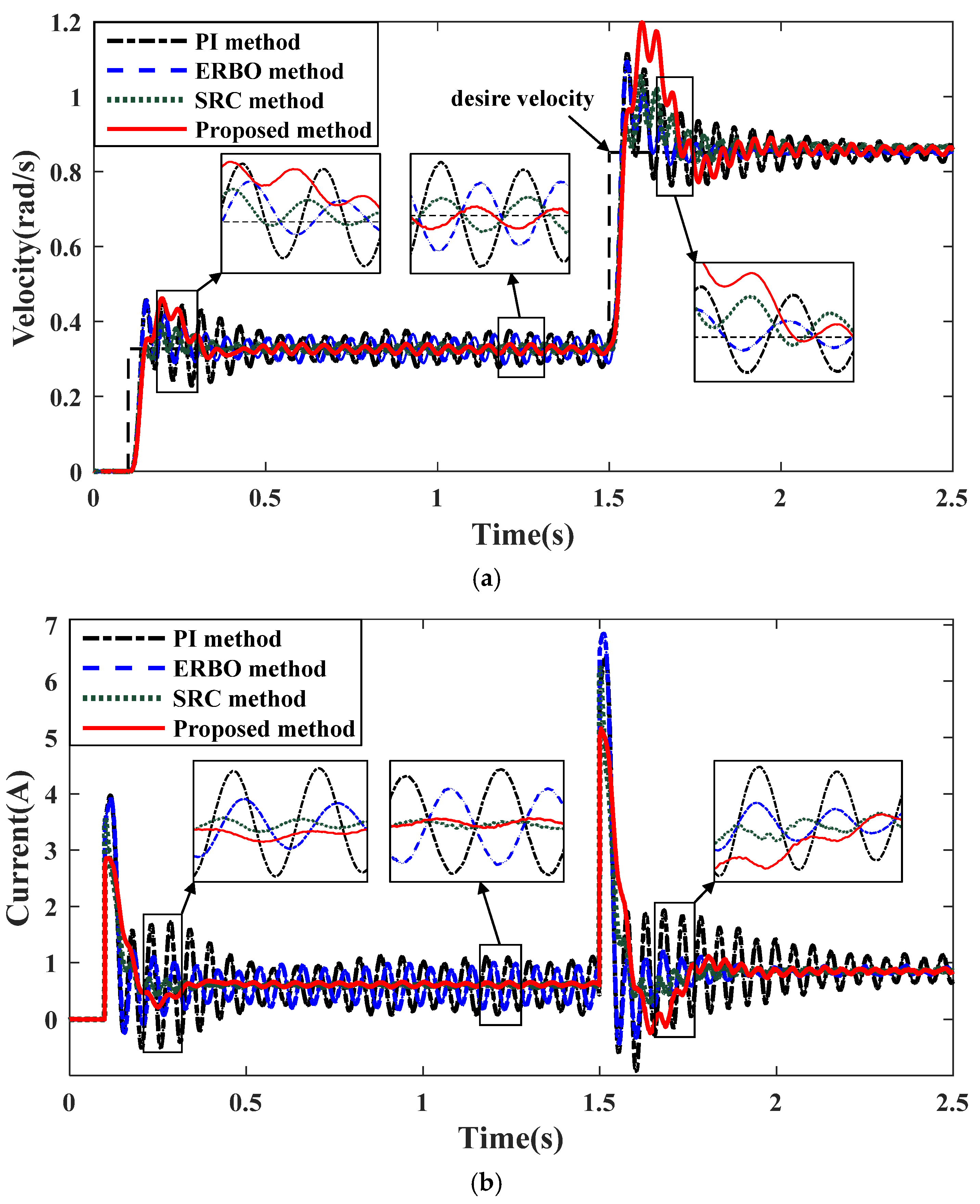
This paper proposes a velocity control method to reduce the sensitivity to model uncertainties and external disturbances near the system resonant frequency, improving the robust stability and velocity tracking accuracy. The proposed method mainly includes a rigid-body state observer and an adjustable damper. The rigid-body state observer is designed the order of its nominal model as similar to the actual physical plant as possible, which lets the gain of this observer be pushed higher. Thereby, the high gain increases the bandwidth of the observer and improves the observation accuracy of the equivalent rigid-body velocity. Notably, the high gain can attenuate the adverse influences of the model uncertainties and exotic disturbances near the resonant frequency. In addition, when the feedback gain of the adjustable damper is tuned to a unique value, the proposed method can be equivalent to the SRC method but be more robust and stable. Ultimately, an adjustable damper combined with the high gain rigid-body state observer adds system damping to simultaneously reduce the residual vibration during acceleration/deceleration and torque ripple during low-speed uniform motion. In order to validate the advantages of this method, the experiments are compared with a PI method and two other rigid-body velocity methods, such as the ERBO method and the SRC method.
The contributions of this paper are:
1. The designed rigid-body state observer can compensate for model uncertainties, such as modeling errors and unmodeled system damping.
2. The designed rigid-body state observer combined with the adjustable damper can improve the robustness to model uncertainties and external disturbances.
3. The proposed method can simultaneously suppress the residual vibration induced by the system resonant frequency during acceleration/deceleration and torque ripple caused by the HD during low-speed uniform motion.
This paper is organized as follows. The modular joint is described and modelled in
Section 2. The controller is designed in
Section 3. The system identification, controller parameters analysis and robust stability analysis are arranged in
Section 4. Next, the experiments and results are discussed in
Section 5. Finally,
Section 6 concludes this paper.
2. System Description and Dynamic Modeling
The modular joint integrates electronics and mechanical components, including a Permanent Magnet Synchronous Motor (PMSM), HD, shaft, bearings, dual encoders (motor-side encoder and link-side encoder), torque sensor, and other components, as shown in
Figure 1.
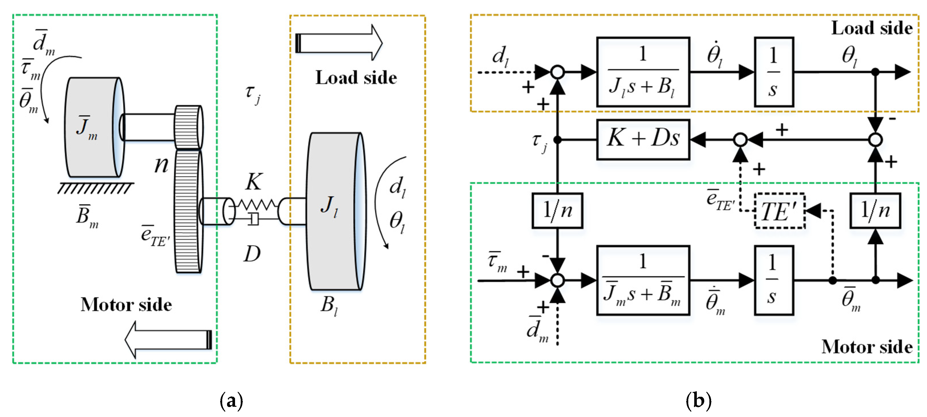
According to
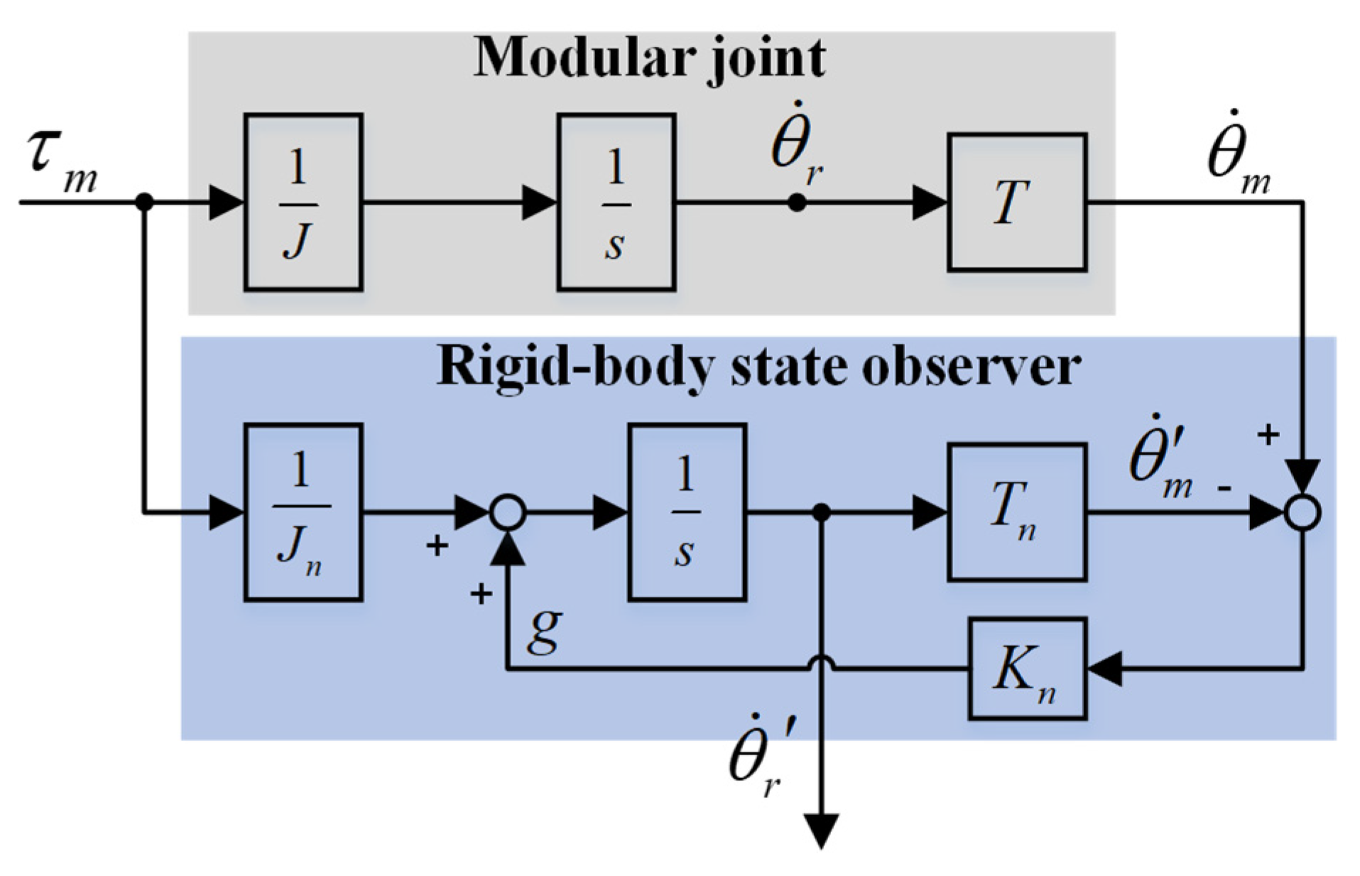
Figure 1, a two-inertia model is employed to describe the physical behavior in
Figure 2a. The mathematical model diagram of the two-inertia model is shown in
Figure 2b. Wherein,
,
,
,
,
,
, and
n are the motor inertia, load inertia, motor viscous damping, load viscous damping, motor position, load position, and reduction ratio of the HD, respectively.
,
indicate the input torque and joint torque. The drive chain (includes torque sensor and HD) is modelled as a linear spring
K and viscous damper
D. Furthermore,
is the motor-side external disturbances, such as the modeling errors, nonlinear frictions, and unmodeled system damping.
dl is the link-side external disturbances, such as the imprecise load inertia and unmodeled nonlinear environmental damping.
is the transmission error of the HD, whose dominant frequency is twice related to the motor velocity [
30].
In general, the dynamic equations of the modular joint are expressed as a two-inertia model, as shown in the following [
31]:
The parameters
,
,
,
,
,
are defined as
,
,
,
,
,
. Therefore, the dynamic equations can be simplified to (2).
Moreover, to further simplify the modular joint’s model, the external disturbances and the transmission error of HD are temporarily omitted. Consequently, the transfer function from input torque
to motor velocity
and link velocity
in Laplace domain are given in (3) and (4), respectively.
where
.
3. Controller Design
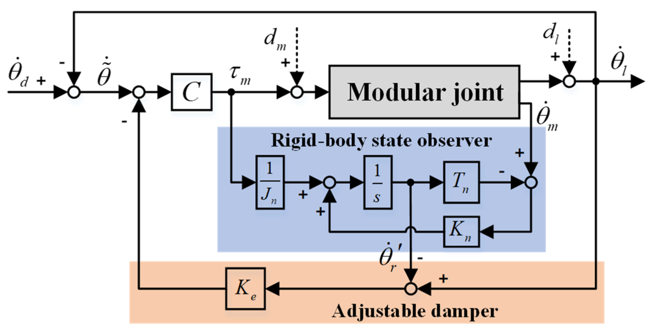
In order to suppress the residual vibration during acceleration/deceleration and torque ripple during low-speed uniform motion, a robust velocity control method is proposed in this paper. The method mainly includes a rigid-body state observer, an adjustable damper, and a controller
C, as shown in
Figure 3. The error between link velocity and rigid-body velocity is additionally fed back beside the link velocity feedback. The motor and link velocity can be acquired from the motor-side and link-side encoders of the modular joint, which is estimated by the differentiation of the motor position and link position. The rigid-body velocity is a nominal velocity of the modular joint, which can be derived from (3) and (4) as
. However, in a two-inertia system, the rigid-body velocity cannot be measured directly by sensors. Therefore, how to acquire the rigid-body velocity is the fundamental issue that needs to be first considered.
A rigid-body state observer is designed to obtain the equivalent rigid-body velocity. Then, based on the designed observer, an adjustable damper feeds back the error between link velocity and the observed equivalent rigid-body velocity to a controller C.
3.1. Rigid-Body State Observer Design
In earlier works, the modular joint system is described as a simplified two-inertia model in (2).
Figure 4 shows the rigid-body state observer, where the nominal model
Jn is the sum of motor inertia and load inertia, expressed as
Jn =
Jm +
Jl. Firstly, we assume that there is no error between the physical model
J and the nominal model
Jn, so
J =
Jn.
The closed-loop feedback value
g of this observer, marked in
Figure 4, can be expressed as:
The transfer function
R from the actual rigid-body velocity
to the observed rigid-body velocity
is given as:
The nominal model Tn is designed as Tn = T in the rigid-body state observer. In this case, the closed-loop feedback value g in (5) becomes g = 0, which means the gain Kn can be infinite theoretically. Similarly, the observed rigid-body velocity always equals the actual rigid-body velocity as R = 1 with any gain Kn in (6). Under the premise of system stability and R = 1, the model uncertainties and external disturbances can be effectively cancelled with a sufficiently high gain Kn.
In order to avoid the identification of
Tn,
Tn is designed to be unity in [
29], where the nominal model of its observer only contains the rigid-body dynamics. In this observer, the closed-loop feedback value
g in (5) becomes:
The transfer function
R in (6) becomes:
From (7), the gain Kn is affected by the resonant frequency, which leads to difficulty in Kn tuning. Particularly, the system may become unstable during high acceleration and deceleration. Thus, the gain Kn has to be small enough to ensure the system stability, which unfortunately causes the poor robustness to model uncertainties and exotic disturbances. In addition, the observed rigid-body velocity in (8) is also influenced by the resonant frequency, which reduces the observation accuracy of the equivalent rigid-body velocity. This further weakens the vibration suppression performance in the outer loop.
Considering the robust stability of the system to model uncertainties and exotic disturbances, the nominal model
Tn is designed as:
Actually, there are unavoidable model uncertainties on the physical plants regarding
J and
T. The rigid-body state observer based on
norm optimization can strictly guarantee robust stability to the model uncertainties [
23]. Suppose that the model uncertainties can be treated as a multiplicative perturbation in (10), where the perturbation
and
are assumed to be stable. So,
J and
T are represented as:
The rigid-body state observer is robust stable if:
where
and
represent the maximum of singular value.
However, the rigid-body state observer is only a part of the overall control system. Robust stability to model uncertainties should be considered with the outer loop. To comprehensively analyze the model uncertainties, define
as the total model perturbation, expressed as:
The transfer function from the output of the total model perturbation
to its input is:
Suppose
is bounded by the upper limit function
as:
Then, satisfaction of the following condition guarantees the robust stability of the whole closed-loop system:
3.2. Adjustable Damper Design
During the adjustable damper design, some assumptions are prepared for simplifying the analysis of the closed-loop performance of the controller. The physical plants
J and
T are assumed to equal the nominal models
Jn and
Tn without model uncertainties, shown as (16).
Under these assumptions, the observed velocity
in the rigid-body state observer is equal to the actual velocity
, directly calculated in (17) without the control parameter
Kn.
Therefore, with the assumptions in (16), the adjustable damper can be designed separately without considering the control parameter
Kn. Define the velocity error
between the desire velocity
and link velocity
as
, marked in
Figure 3. Thus, the open-loop transfer function from
to
is given as:
The closed-loop transfer function from
to
is given as:
Compared (19) with (18), the closed-loop transfer function adds a damping term–KeCs to the modular joint system. As the gain Ke is negative, the system damping is increased. When the modular joint moves during acceleration and deceleration, the added damping term can suppress the residual vibration. Meanwhile, the increased system damping also can eliminate the torque ripple during the low-speed uniform motion to advance the velocity tracking accuracy.
In addition, the modular joint also experiences external disturbances, including motor-side exotic disturbances
dm and link-side exotic disturbances
dl, as shown in
Figure 3.
The sensitivity function
DM from
dm to
is:
where
,
,
,
.
The sensitivity function
DL from
dl to
is:
where
,
,
,
.
These external disturbances unavoidably degrade the velocity control accuracy, especially when the tracking velocity changes sharply. Therefore, the robustness to external disturbances near the resonant frequency should be considered.
4. Controller Analysis
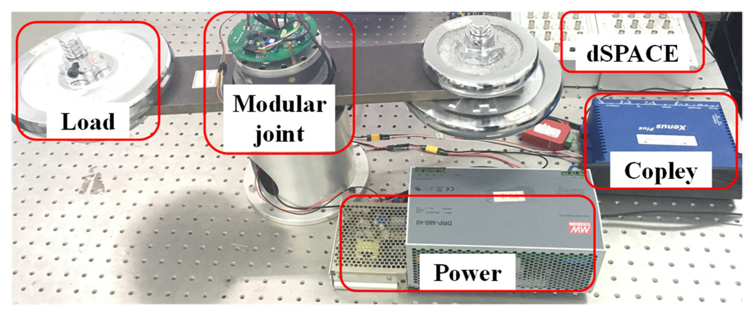
To analyze the proposed controller’s robustness performance and velocity tracking accuracy, the dynamic parameters of the controlled object—modular joint need to be identified first. The modular joint installed some loads is publicized in
Figure 5. The installed loads compose the modular joint’s load inertia.
4.1. System Identification
The experimental platform includes a modular joint, a 24 V power, a Copley driver, a dSPACE real-time control system, several loads, and a MATLAB data processing system, as shown in
Figure 5.
The sampling frequency is set as 1 kHz. The gear ratio n of HD is 160. The torque constant of motor is 0.17 N·m/A. The input saturation current is set to be 10 A. The maximum allowable desire velocity is 1.64 rad/s. The motor velocity and link velocity are obtained by the differentiation of the motor position and link position, which are measured by the motor-side encoder and link-side encoder, respectively.
A swept sine signal from 0.5 Hz to 60 Hz with a load inertia
Jl = 2.26 kg
·m
2 is applied to identify the modular joint’s open-loop dynamic characteristics. According to system identification results, the modular joint’s frequency responses from input torque to motor velocity and link velocity are displayed in
Figure 6a,b, respectively.
The blue dash-dot lines are the results of the system identification experiments. The red thick solid lines are fitted frequency responses of the established two-inertia model. Whereas, the actual modular joint’s dynamic model is subjected to several nonlinear and time-varying factors, such as the nonlinear frictions and viscous damping effects in the motor-side and transmission part, and the varying efficiency of the HD (60–75% depending on ratio, velocity, and lubricant). In particular, the stiffness and damping of the HD are related to the motion velocity. Therefore, the established two-inertia model cannot accurately fit the experimental results, especially the phase [
32]. However, the system’s anti-resonant frequency and resonant frequency can be well fitted at 19 Hz and 21.8 Hz, proving that the two-inertia model can reflect the joint’s dynamic characteristics. The dynamic parameters of the modular joint can be identified in
Table 1.
4.2. Controller Parameters Analysis
To meet the rapid response of the modular joint, it is necessary first to ensure the velocity response performance. Based on the Integral of Squared Error (ISE) criterion [
33], the controller
C is designed as a proportional and integral controller, tuned as
Kp = 160 and
Ki = 1200.
Since the rigid-body state observer and the adjustable damper are designed separately, the control parameter
Kn of the observer and
Ke of the adjustable damper can also be designed separately. As the rigid-body state observer is shown in
Figure 4, the transfer function from motor velocity
to the observed velocity
can be expressed in (22).
With the identified modular joint’s dynamic parameters listed in
Table 1, the bode plots from motor velocity to the observed velocity are obtained under the different control parameter
Kn in
Figure 7. With the gain
Kn increasing from 100 to 1000, the bandwidth of the rigid-body state observer increases.
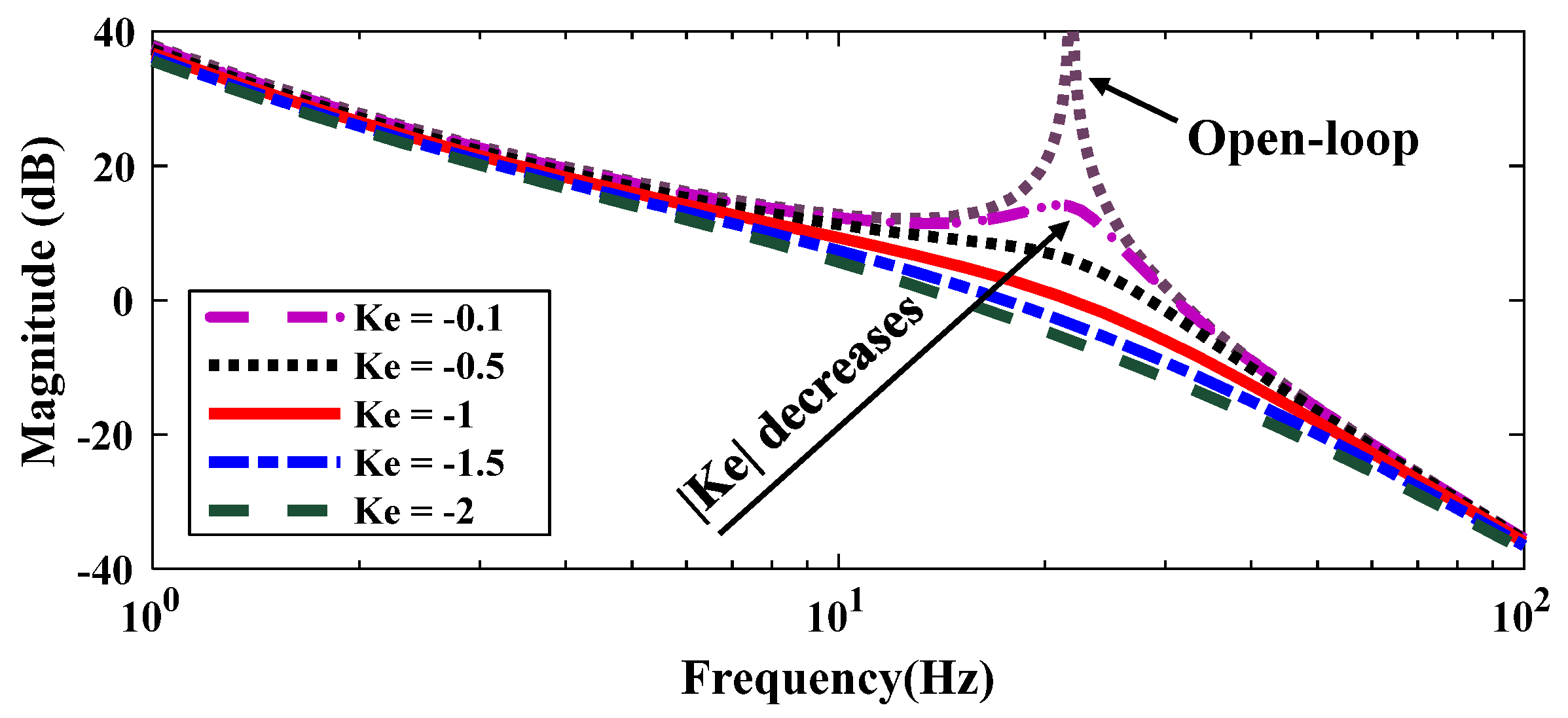
In addition, as the value of the control parameter
Ke changes, the open-loop and closed-loop frequency responses from velocity error
to link velocity
are shown in
Figure 8. With the absolute value of the gain
Ke increasing, the vibration magnitude at resonant frequency decreases accordingly. When the added damping is too small, such as
Ke = −0.1, the vibrations cannot be suppressed effectively because of the limited damping added. When the added damping is too large, such as
Ke = −2, the system response slows down, meanwhile low-frequency uncertainty increases.
The most conservative condition to ensure the controlled system is stable with little vibration is to let the amplitude ratio of the closed-loop frequency response in (19) be 0 dB at the resonant frequency, as expressed in (23).
The theoretical value of
Ke from (23) can be calculated as −1. Considering the model uncertainties and nonlinear damping effects, the parameter
Ke needs to be adjusted in a small range around −1 in actual experiments. Most importantly, in order to meet the robust stability condition of the whole closed-loop system as designed in (15), the controller’s parameters of the proposed method are designed in
Table 2.
4.3. Robust Stability Analysis
Further to analyze the robust performance of the rigid-body state observer, the model perturbations of Jn and of Tn are separately considered. In this paper, the model uncertainties mainly refer to the modeling errors, unmodeled system damping, system identification errors, even the imprecise motor and load inertia.
is the transfer function from the output of the model perturbation
to its input.
is the transfer function from the output of the model perturbation
to its input. With the proposed method, the transfer function
and
can be expressed as (24) and (25), respectively.
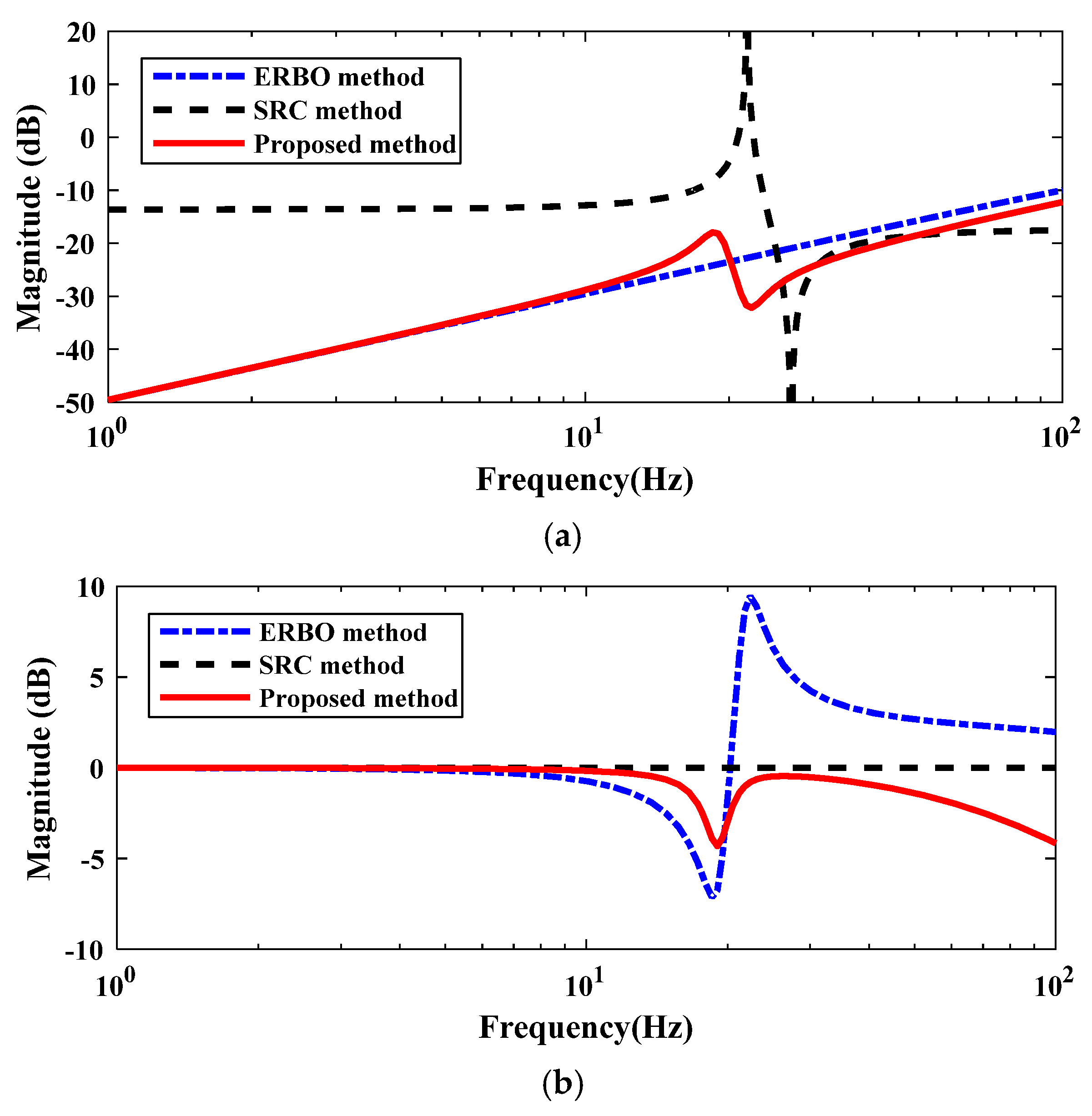
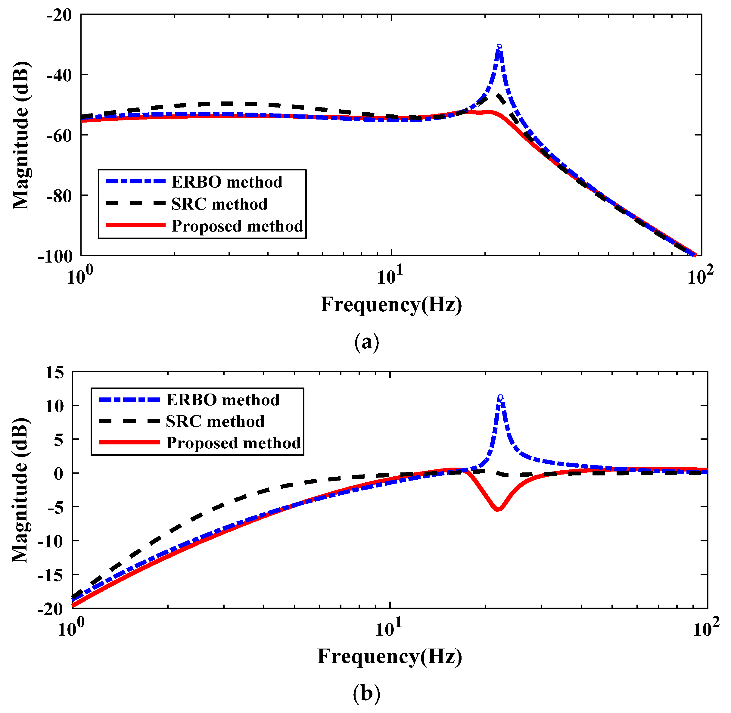
For a fair comparison, optimal controller parameters are employed in the ERBO method, SRC method, and the proposed method, respectively. The bode plots of the transfer function
and
with these three methods are compared in
Figure 9a,b, respectively.
From
Figure 9a, the SRC method is susceptible to the model uncertainties of
Jn, especially at the low-frequency band and anti-resonant frequency. Compared with the ERBO method, the proposed method reduces the sensitivity to the model uncertainties near the resonant frequency, increasing system robustness. Although it improves the sensitivity near anti-resonant frequency, the characteristic of anti-resonance makes the system unresponsive, which means this introduced shortcoming is not that serious.
From
Figure 9b, the ERBO method is susceptible to the model uncertainties of
Tn, especially near the resonant frequency and high frequency. The SRC method is derived from the model
Jn in an open-loop, which is little related to the model uncertainties of
Tn. Compared with the ERBO and SRC methods, the proposed method significantly reduces the sensitivity to model uncertainties near the resonant frequency and high frequency.
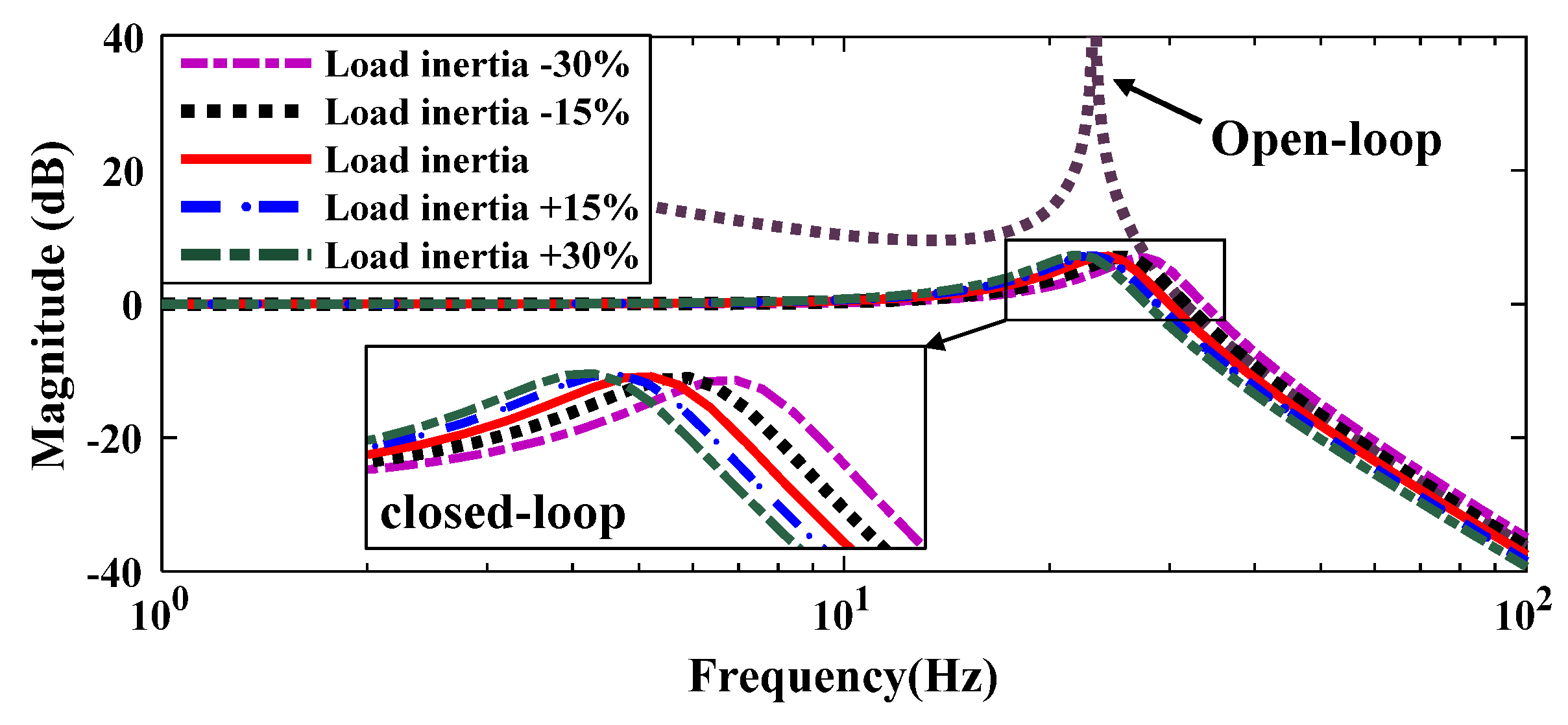
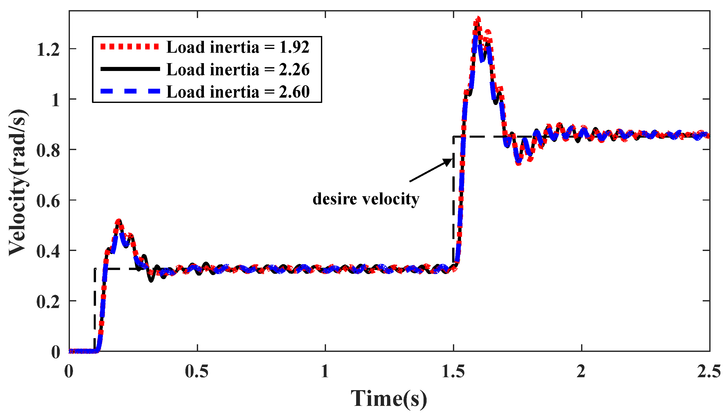
In addition, robust performance to model uncertainties can be verified with a specific physical indicator. Under the premise of ensuring that the dynamic parameters in
Table 1 and controller parameters in
Table 2 remain unchanged, the total model perturbation
is simulated by changing the load inertia. The closed-loop transfer function from desire velocity
to link velocity
is expressed in (26).
As the load inertia changes within
Jl ± 30%, the frequency response of the closed-loop transfer function in (26) is shown in
Figure 10.
Compared to the open-loop frequency response, the oscillation magnitude of closed-loop near resonant frequency can be damped effectively. With the load inertia increasing, the system resonant frequency decreases accordingly. It is obvious that the closed-loop system is robust and stable to the load inertia changing.
What’s more, the modular joint is also influenced by the motor-side and link-side external disturbances. In order to analyze the robustness to external disturbances of the proposed method,
Figure 11a,b, respectively, show bode plots of the sensitivity functions
DM and
DL, expressed in (20) and (21). The ERBO method and SRC method are also compared and discussed following.
In particular, according to the feedback signals, when the feedback gain Ke of the adjustable damper is tuned to −1, the proposed method can be equivalent to the SRC method. Fortunately, the proposed method contains a closed-loop rigid-body state observer and an adjustable damper, which ensures the system robust stability performance. Justifiably, from the bode plots of these three methods, the SRC method behaves with the worst robustness on the low-frequency domain. The ERBO method behaves with the worst robustness near the resonant frequency. Compared with the SRC method and ERBO method, the proposed method is the most robust to the external disturbances, especially near the resonant frequency, which means its ability to work against exotic disturbances during high acceleration and deceleration is stronger than the other two methods.


