1. Introduction
Currently, there are many computer modeling problems that require reduction to the class of optimal control problems (OCP) to automate the process of finding a solution, as well as to reduce the complexity of calculations. The most common tool for solving such problems is numerical methods, including the apparatus of artificial neural networks (ANN). The advantage of ANN is the ability to construct a solution in the form of a functional dependence with high accuracy [
1,
2]. At the same time, the use of other numerical optimization methods requires the subsequent interpolation of the discrete solution, which, in turn, imposes an additional error. In addition, the efficiency of using the neural network approach for solving the OCP is expressed in the possibility of obtaining a solution not only satisfying the necessary optimality conditions, but also smoothness conditions.
In the study [
3], A. Nazemi and R. Karami presented the main stages of solving OCP with mixed constraints. Based on the optimal Karush–Kuhn–Tucker conditions, the authors constructed a function for calculating the error and formulated a nonlinear optimization problem, in which neural network approximations are defined for the state function, control, and Lagrange multipliers. For the obtained scheme of dynamic optimization of the weight coefficients of the neural network solution, the analysis of stability and convergence is carried out.
The most relevant application of the neural network approach is in cases where the solution of optimal control problems does not have an analytical solution [
4] or the type of analytical solution cannot be determined directly [
5,
6]. In addition, the approach under study does not require the search for the optimal ratio of the step size along the axes under consideration, in contrast to finite-dimensional methods [
7].
In the study [
8], the authors T. Kmet and M. Kmetova considered the use of ANN for solving an OCP with a free end time and constraints on control and phase trajectory. Note that the construction of the corresponding nonlinear programming problem was carried out on the basis of neural network control using adaptive criticism. The proposed approach demonstrated the effectiveness in the field of optimal management of photosynthetic production and confirmed the relevance of the introduction of an adaptive critical system approach.
The authors of the study [
9], F. Kheyrinataj and A. Nazemi, presented a numerical method for solving the OCP with fractional delay, which implements nonlinear polynomial expansions in a neural network with an adaptive structure. The developed neural network approach has demonstrated its effectiveness in many specific examples.
The presented neural network solutions, as well as other modifications of the ANN for solving the OCP [
10,
11,
12], can be combined and the main advantage can be highlighted—the presentation of the problem solution as continuous over the entire domain of definition, while the rest of the numerical methods allow you to find values directly at discrete points and require interpolation to calculate the values between them [
13]. In addition, with an increase in the number of partitions of the original domain of definition [
14] and the dimension of the problem [
15], as a rule, the computational complexity does not increase significantly.
In this paper, we consider the computational features of the neural network approach to solving optimal control problems using various methods of evolutionary optimization. This paper describes the structure of a neural network solution that satisfies the Kreinovich theorem and corresponds to a hole-layer perceptron, and also presents a general scheme for optimizing its parameters. This area of research is relevant, since the use of evolutionary algorithms in many applied areas [
16,
17,
18,
19] has made it possible to increase the efficiency of finding optimal values even in the case of analyzing functions that have many local optima or do not have a clear global optimum.
Note that the evolutionary algorithms not only allow us to obtain well-interpreted results, but also quite simply combine with other methods [
20,
21,
22]. At the same time, these algorithms do not provide a strict finding of the optimal solution in a finite time and require adjustment of the parameters of the models used [
23,
24,
25]. Thus, evolutionary algorithms are heuristic, that is, the accuracy and rigor of the solution do not prevail over the feasibility. In this regard, the use of this type of optimization methods in solving applied problems requires a more detailed analysis.
In this regard, this study is aimed at studying the computational features of the neural network approach to solving optimal control problems with mixed constraints using evolutionary optimization algorithms: the genetic algorithm, the gravitational search algorithm, and the basic particle swarm algorithm. Thus, this paper is devoted to the study of the neural network approach to solving optimal control problems and optimizing the structure of the functional representation by evolutionary algorithms in order to analyze their efficiency and convergence rate. This paper contains examples of optimal control problems that have an analytical solution and allow us to evaluate the convergence of the algorithms under study.
The rest of the paper is organized as follows:
Section 2 describes a formal mathematical formulation of the optimal control problem with mixed constraints.
Section 3 presents a neural network model for approximating the optimal control problem, as well as a description of the studied evolutionary algorithms for optimizing the neural network solution. In
Section 4, the practical implementation of the presented algorithms is presented and the results are evaluated.
2. Necessary Optimality Conditions for OCP with Mixed Constraints
Consider the general formulation of the optimal control problem corresponding to the Bolza problem with mixed constraints. Let us introduce function , which describes the development of a certain system. Function is called a state variable (or trajectory) satisfying the continuity condition.
Note that for the system at the initial moment of time the state is known:
We will assume that the further dynamics of the system depends on some particular choice (or strategy) at each moment of time and this strategy is given by function . A fixed set in is called a control set, and function is called a control function.
Based on the fact that
determines the development of the system, the dynamics of the state variable will take the form:
where
and function
belongs to the space of continuously differentiable functions
.
We say that a piecewise continuous function is an admissible control for (1)–(2) if there is a unique solution to this ordinary differential equation, defined on , and solution is called the trajectory corresponding to control .
In addition, for each system, control constraints can be described in one way or another. Within the framework of this study, it is assumed that there are mixed constraints for the system, simultaneously linking control and a state variable:
Let function describe variable costs (or operating costs, variable payments, etc.). Let the values of be fixed.
Consider the set
of admissible controls and define the quality criterion
as follows:
which describes the variable costs over the entire time interval and the trajectory constraints at the end of the time interval. Suppose that functions
and
also belong to the space of continuously differentiable functions, i.e.,
and
.
The optimal control problem (1)–(4) is a Bolza problem with mixed constraints, a free right end of the trajectory, and a fixed end time.
One of the most effective approaches to solving problems in optimal control theory is the Lagrange multiplier method. This method consists in reducing the original OCP to the solution of the problem of minimizing the corresponding Lagrange function:
where
.
Then, based on the necessary optimality conditions, it can be argued that the optimal control
, the corresponding trajectory
, and the Lagrange multipliers must satisfy [
3]:
The dynamics of the state variable;
Conditions of stationarity with respect to
and
, respectively:
Additional non-rigidity conditions;
Transversality conditions;
To simplify the solution of this system, we write down constraints (6)–(8) in an equivalent form. To do this, we introduce the concept of an NCP function that satisfies the nonlinear complementarity problem (NCP):
To do this, we introduce the concept of the perturbed NCP-function of the Fischer–Burmeister:
Using the perturbed NCP-function
, we transform conditions (6)–(8) into equality-type constraints in the form:
Thus, the initial OCP is reduced to the problem of nonlinear optimization (6)–(8), (12)–(13), (16), which must be solved by means of neural networks. Consider the process of building a neural network model that approximates the solution to a nonlinear optimization problem.
3. Building a Neural Network Structure for Solving OCP
We represent the functional approximation as a sum of two parts based on two facts. The first term contains no tunable parameters and satisfies the initial or boundary conditions. The second term uses one output direct neural network with adjustable parameters and input signals.
It should be noted that in the second case, the weighting coefficients are adjusted, taking into account the minimization problem and are constructed so as not to contribute to the initial or boundary conditions. Based on these facts and using the neural networks, functional approximations of solutions for the phase trajectory, Lagrange multipliers and control for the system (6)–(8), (12), (13), and (16) can be defined as follows:
where functions
have a structure:
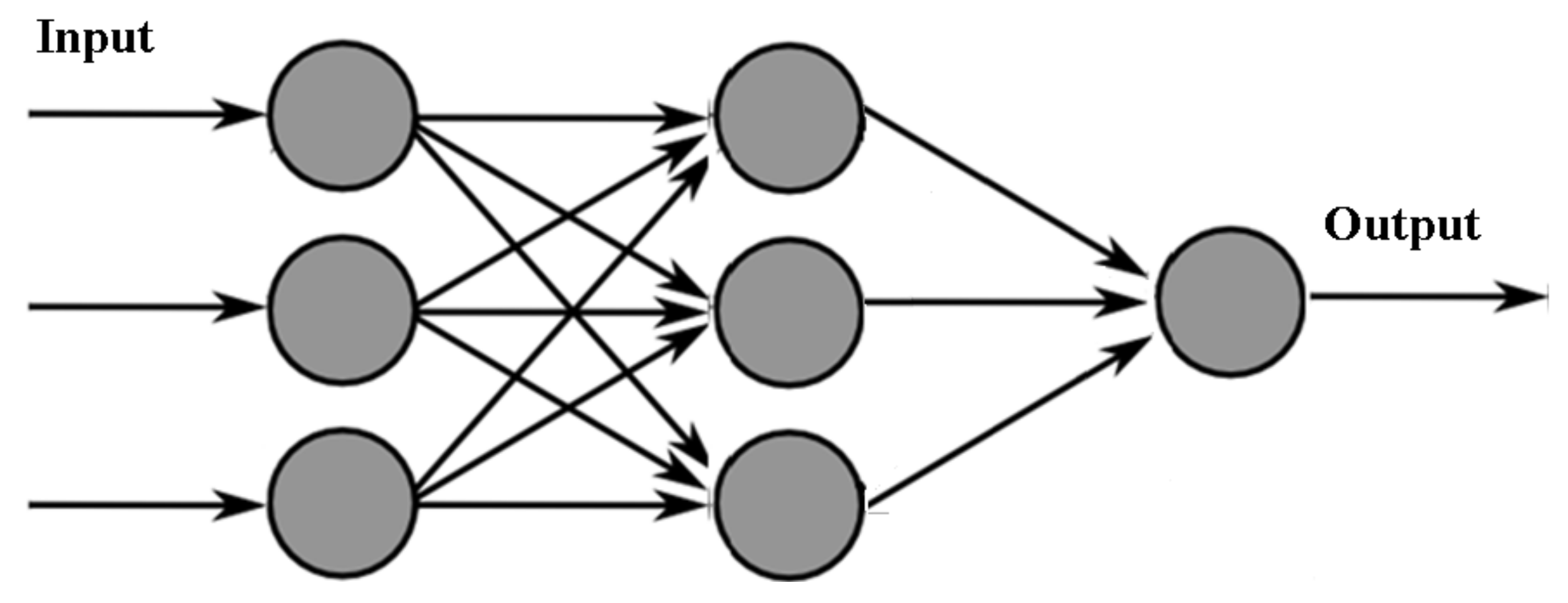
The described structure (18) corresponds to a neural network with a single hidden layer. The input signals
, passing through the neurons of the network and multiplying by their weight coefficients
, eventually form a single weighted feature
. The weighted trait
is further transformed using the activation function (some nonlinear converter) and forms the ANN output for the neuron on the next layer
(
Figure 1). At the output layer, the values of the neurons are multiplied by the weight coefficients of the next layer
, and the response (the output of the ANN) is considered to be the resulting weighted sum.
Thus, the function
has the form:
where
is the number of neurons on the input layer,
is the number of neurons on the next layer.
The task is to select the optimal parameters of the ANN in such a way that the approximated function (17) satisfies the system (6)–(8), (16) with some error. The parameters of the ANN are the number of neurons in the input and output layers, their weight coefficients, and the activation function used.
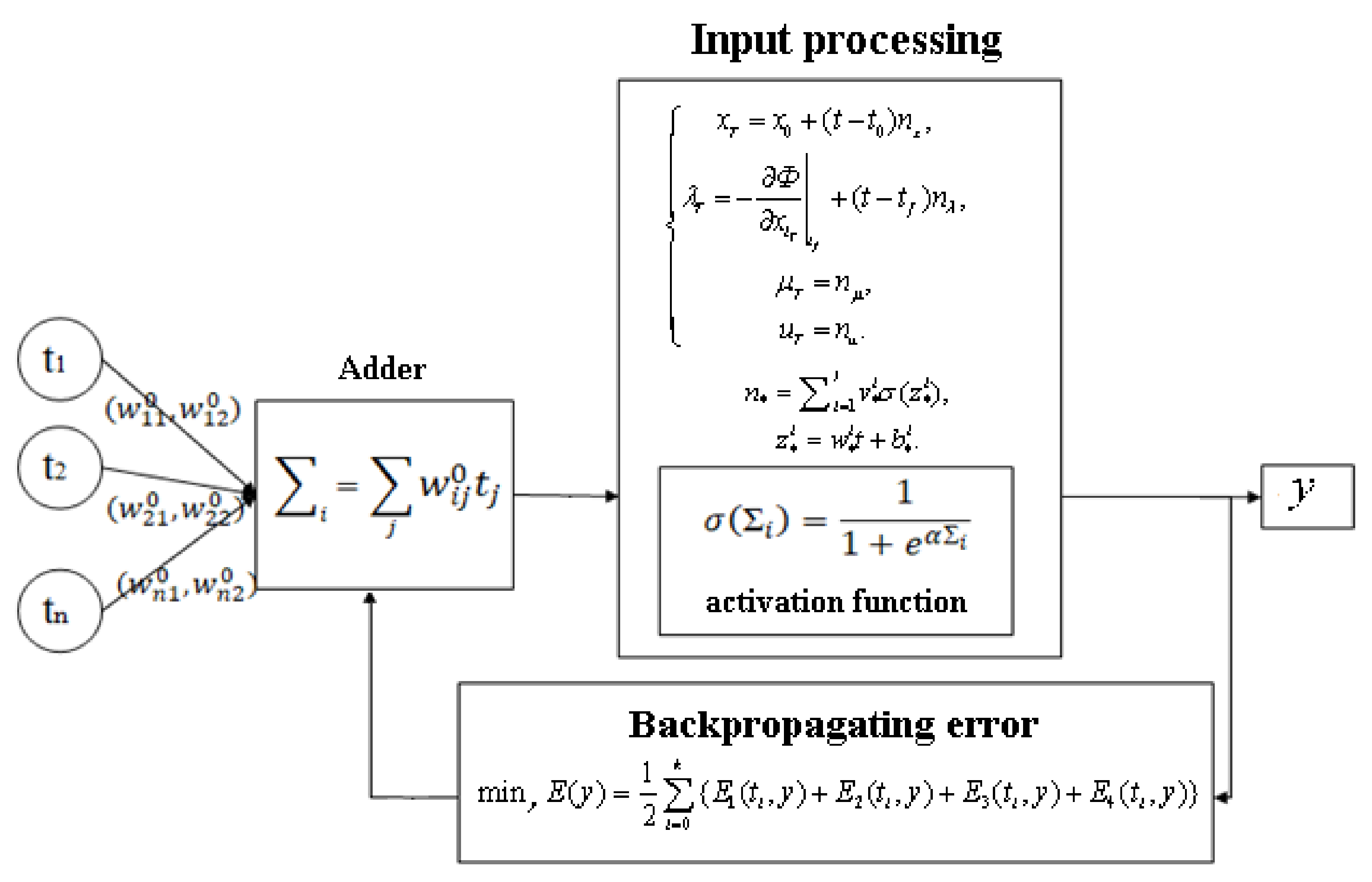
The selection of the optimal weight coefficients of the ANN can be carried out using the algorithm of back propagation of the error, for which it is necessary to create an appropriate optimization problem.
We represent the system of Equations (6)–(8), (16) as an optimization problem: we divide the time interval
into
equal parts by points
, then, based on the least squares method, we have the following formulation of the problem:
where
and
The finite-dimensional optimization problems (19) and (20) makes it possible to use various solution methods and select weight coefficients with a given accuracy for constructing a neural network approximation.
Thus, the ANN weighting coefficients are updated by optimizing the error function (19) by the error backpropagation algorithm, which can be schematically represented according to
Figure 2.
3.1. General Optimization Scheme for A Neural Network Solution
Figure 2 shows a flowchart of a neural network solution (NNS) optimization process, and its specific steps are presented in Algorithm 1.
| Algorithm 1 Optimization of a NNS |
| | Input: NNS,, |
| | Output: |
| 1 | ; |
| 2 | ; |
| 3 | ; |
| 4 | update weight coefficients ; |
| 5 | ; |
| 6 | if orthen
go to step 7;
else and go to step 4; |
| 7 | Return. |
Thus, the efficiency of the neural network solution search depends on the algorithm used to update and optimize the weight coefficients. This study analyzes the accuracy and convergence rate of a neural network approach with various evolutionary optimization algorithms: a genetic algorithm, a population gravity search algorithm, and a basic particle swarm algorithm. The constructed neural network approximations by various optimization methods are compared with the gradient descent algorithm.
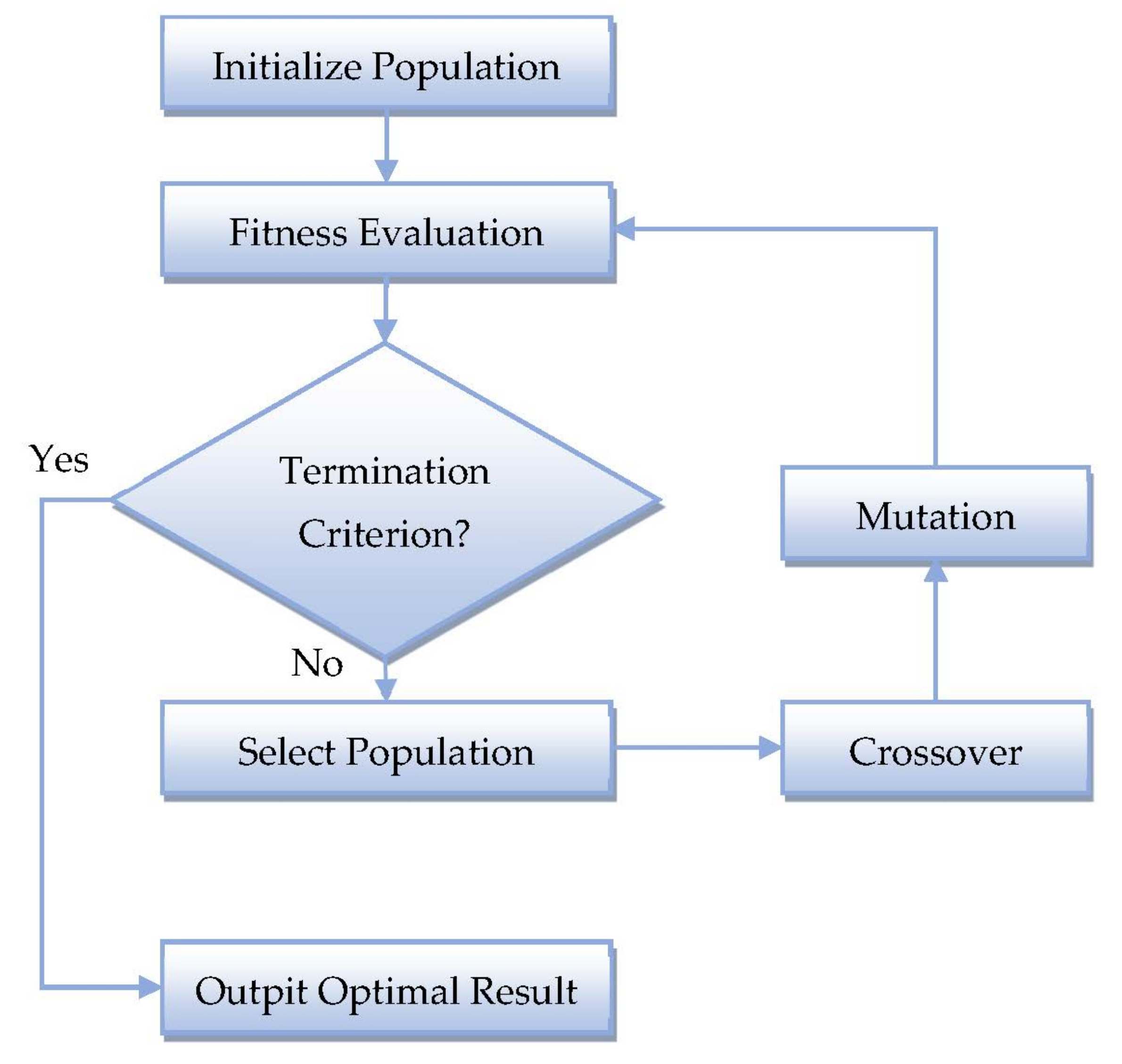
3.2. Genetic Optimization Algorithm
Genetic algorithms search for the solution space of a function using simulated evolution, i.e., the survival of the most complex strategy. At the same time, the fittest individuals of any population tend to reproduce and survive until the next generation, thereby improving subsequent generations. However, lower individuals may accidentally survive and also reproduce.
Research has shown that genetic algorithms solve linear and nonlinear problems by exploring all areas of the state space and exponentially exploiting promising areas through mutations, crossovers, and selection operations applied to individuals in a population. A more complete discussion of genetic algorithms, including extensions and related topics, is presented in [
26].
The genetic algorithm used in this study is shown in
Figure 3.
To apply this algorithm, we define a population of size S as a set of different weights of the neural network approximation.
The fitness function for each set of ANN weights is the minimized error function (19) and (20), which ensures the fulfillment of the necessary optimality conditions.
The optimal set of ANN weighting parameters is such that the error of the approximation function is equal to the given computational accuracy.
The mutation operation is performed as a change in some weight by a random set of values.
The crossing of one set of weight coefficients with another is determined using one-point crossing over.
Selection (selection of the best individuals in the population) is carried out by preserving a certain percentage of the best individuals in the new generation.
The optimization process will go on until the specified computation error is reached.
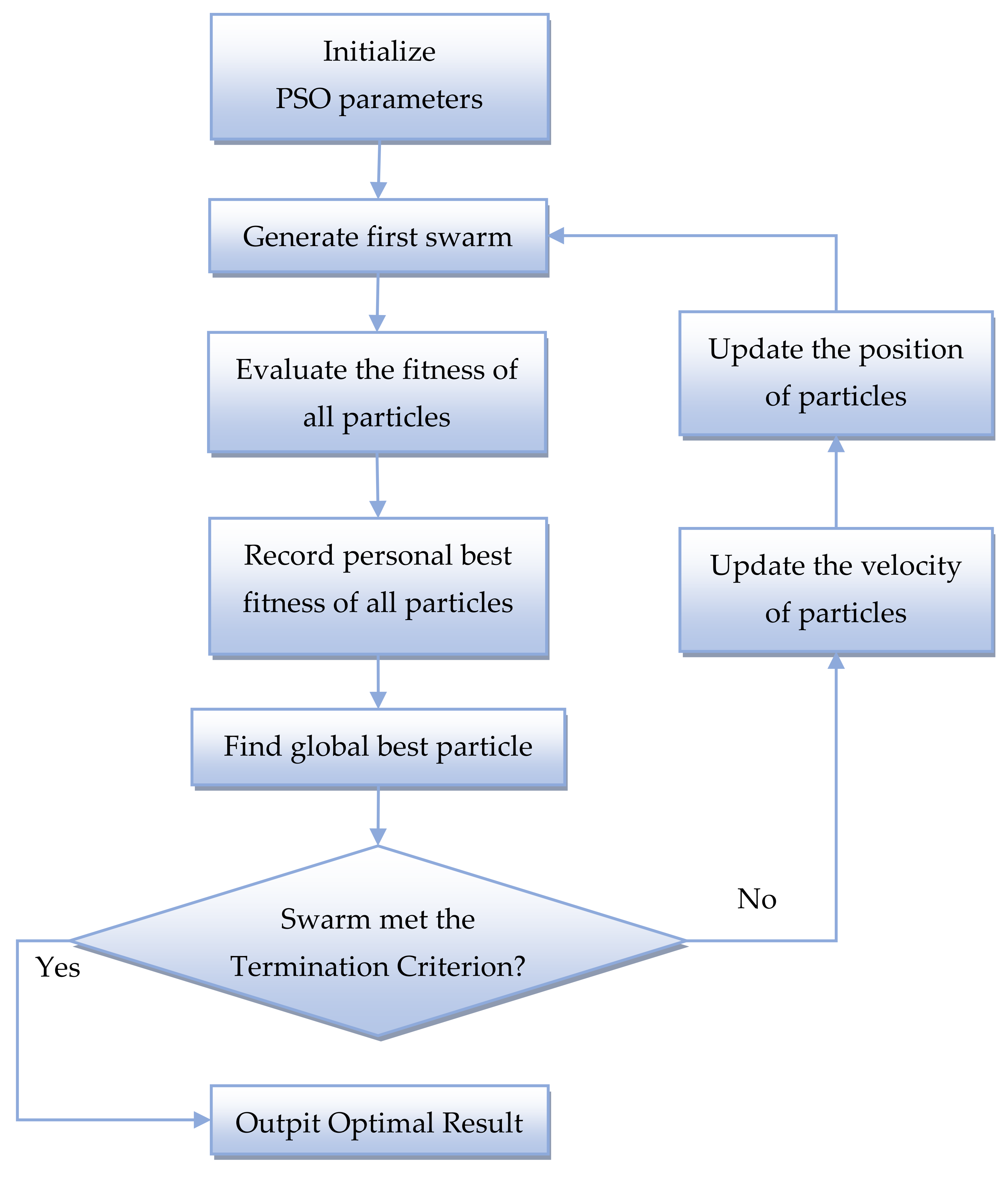
3.3. Basic Particle Swarm Algorithm
The main idea of the particle swarm algorithm [
27,
28] is to move the population of possible solutions in the direction of the best found position of the particles (solution). This algorithm belongs to the class of multi-agent methods.
| Algorithm 2 Basic Particle Swarm Algorithm |
| | Input: |
| | Output: |
| 1 | ; |
| 2 | ; |
| 3 | if then
to step 13;
else and to step 3; |
| 4 | ; |
| 5 | ; |
| 6 | ; |
| 7 | ; |
| 8 | ; |
| 9 | if then
adjust ; |
| 10 | ; |
| 11 | ; |
| 12 | if then
and go to step 4;
else go to step 3; |
| 13 | Return. |
At the initial moment of time, the particles are located chaotically throughout the space and contain a randomly specified velocity vector. For each particle located at a certain point, the value of the fitness function is determined and compared with its best location, as well as the best location relative to the entire population.
At each iteration, the direction and value of the particle velocity is corrected, relying on the approach to the best point among a given number of neighbors, as well as on the approach to the global optimum point. The proposed method is aimed at the fact that after a finite number of iterations, a larger number of particles will be located near the most optimal point. The particle swarm algorithm is shown in the flowchart in
Figure 4, and its specific steps are shown in Algorithm 2.
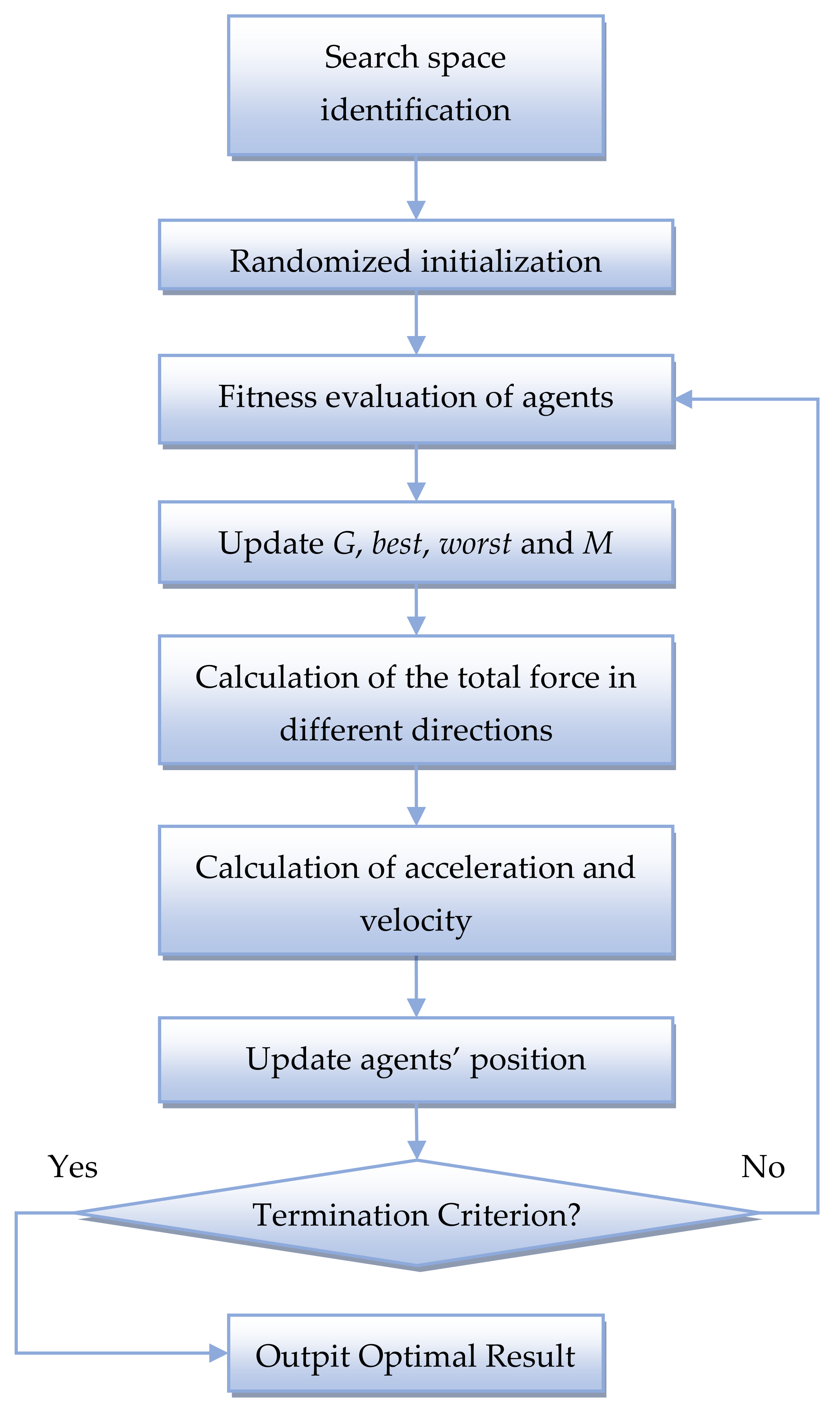
3.4. Gravitational Search Algorithm
Similarly to the previous method, the gravitational search algorithm [
29,
30] moves the population of possible solutions; however, the direction of movement is set based on the relationship of particles according to the principles of the laws of gravity and mass interaction.
The gravitational search algorithm (
Figure 5) uses two laws:
The law of gravitation: each particle attracts others and the force of attraction between two particles is directly proportional to the product of their masses and inversely proportional to the distance between them. Note that, unlike the Universal Law of Gravitation, the square of the distance is not used, which provides the numerical algorithm with more efficient results.
Law of motion: the current speed of any particle is equal to the sum of the part of the speed at the previous moment of time and the change in speed, which is equal to the force with which the system acts on the particle, divided by the inertial mass of the particle.
The gravity search algorithm is presented in Algorithm 3.
| Algorithm3 Gravitational Search Algorithm |
| | Input: is small constant |
| | Output: |
| 1 | are random variables uniformly distributed from zero to one; |
| 2 | for i = 1:N do
;
end |
| 3 | update the gravitational constant, best and worst particles, and masses
for
end |
| 4 | |
| 5 |
end
end |
| 6 |
end |
| 7 |
end |
| 8 | |
| 9 | if then
go to step 10;
else go to step 2; |
| 10 | Return. |
All the optimization algorithms proposed in this study have various advantages and disadvantages presented in
Table 1. Due to the fact that the investigated optimal control problem has been transformed into an equivalent problem of nonlinear optimization of a function of many variables, it is impossible to unambiguously identify the most efficient of the algorithms based on theoretical assumptions.
4. Computational Experiments
Earlier in our research, we showed that the application of the neural network approach to solving optimal control problems demonstrates good results for the OCP with the Lagrange function linear with respect to the control. An analysis of the application of various optimization algorithms for neural networks for solving linear OCPs showed that the evolutionary optimization algorithm uses the least number of iterations to achieve a given accuracy.
Within the framework of this study, we will consider the class of quadratic optimal control problems and analyze the behavior of the considered optimization methods in this case. In addition, within the framework of this study, an example of the OCP for which algorithms are stuck at a local optimum of the considered algorithms falling into the local extremum of the optimized function is given, for linear OCPs.
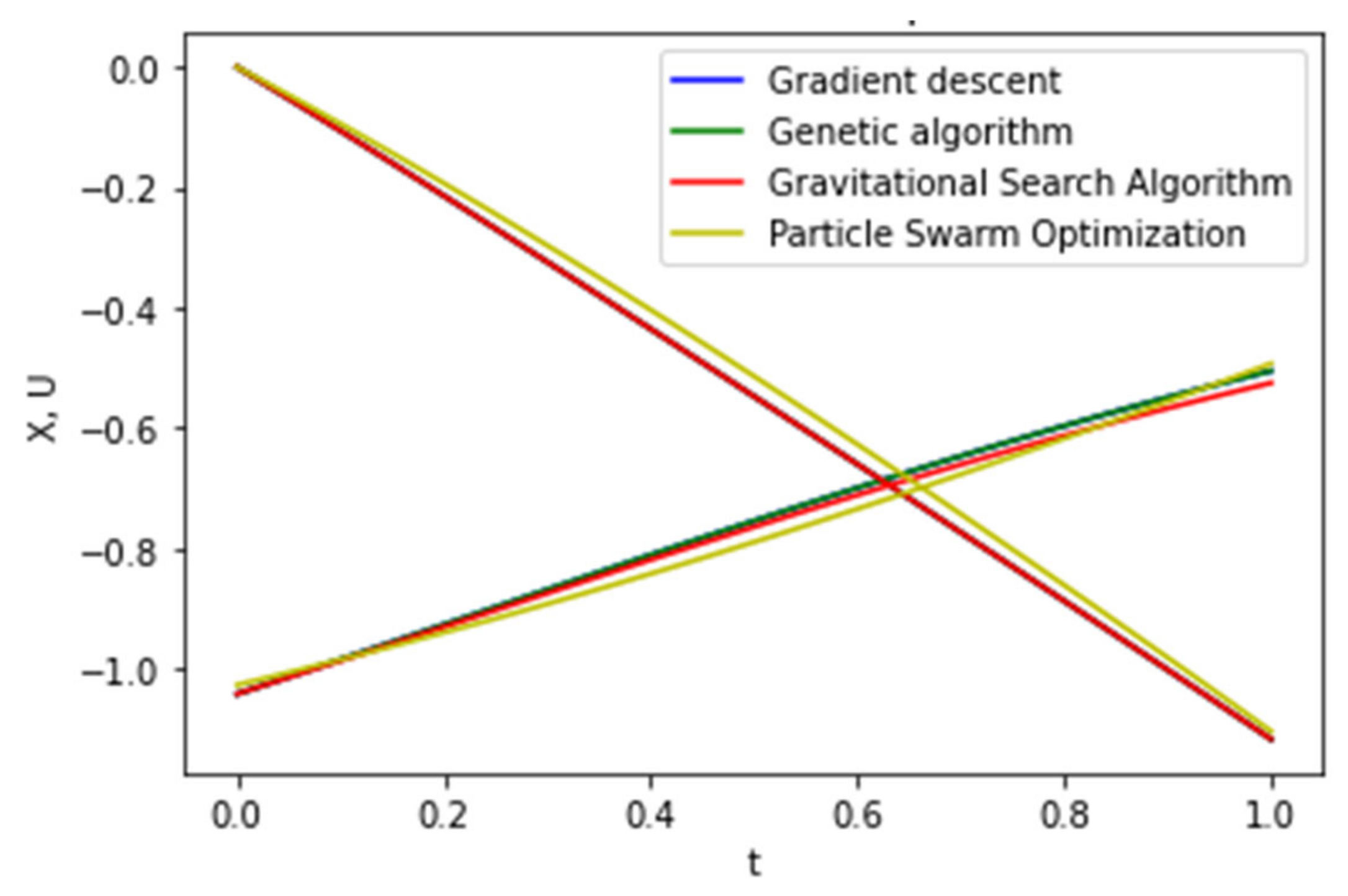
Example 1. The Quadratic OCP.Consider a particular OCP with a quadratic functional with respect to a control of the form:
Let us compose the Lagrange function corresponding to problem (21):
The corresponding optimization problem (21) has the form:
where
and
We define functional approximations of the neural network taking into account the boundary conditions in the form:
Let us compare the results of the neural network approach of finding a solution to the OCP using various methods for optimizing weight coefficients. The initial data for the implementation of the algorithms are presented in
Table 2.
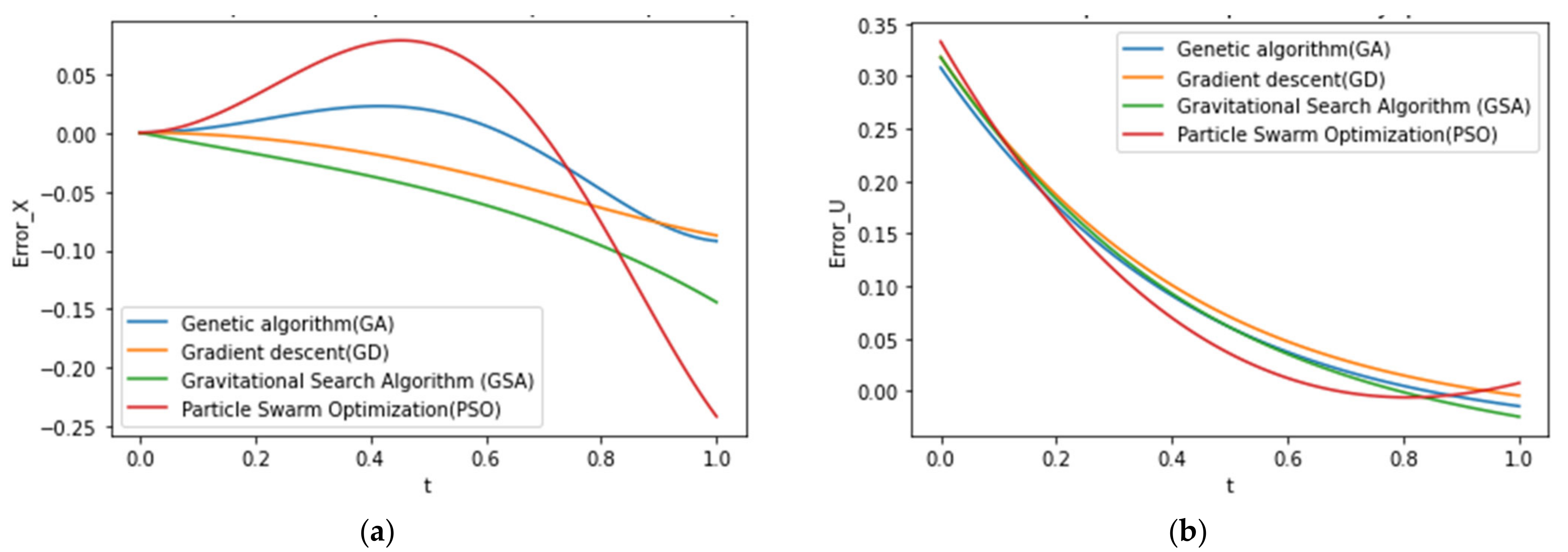
Figure 6 shows neural network solutions to the optimal control problem (21).
Figure 7 shows graphs of errors (deviations of functional approximations from the analytical solution) over the entire time interval along the phase trajectory and control, respectively. The calculated errors of the target functional of the neural network approximation, as well as the values of the additive error of the optimal pair are presented in
Table 3.
The results of the study showed that to achieve a given accuracy, the gradient descent algorithm requires the largest number of iterations , but this method allows achieving better accuracy for the phase trajectory and functional.
The genetic algorithm () has the lowest convergence time among the considered methods for solving OCP (21). In this case, the accuracy of the solution differs from the gradient algorithm in the second order.
The results of the evolutionary gravity search algorithm showed comparable results in terms of accuracy, but the number of iterations required to achieve it is greater than the genetic algorithm. The basic particle swarm algorithm did not get the specified accuracy () and hit the local optimum for the number of iterations .
Note that the view of the deviation graphs of the neural network approximation for various optimization methods confirms that the gradient descent algorithm and the genetic algorithm showed better calculation accuracy. The least accurate functional approximation of the phase trajectory is constructed using the particle swarm algorithm and has an average deviation of the phase trajectory . These function values are the best result of the approximation model approximation (25) obtained experimentally for the PSO method. The results obtained can be explained by the disadvantage of the PSO algorithm in the absence of procedures for exiting local optima, as well as the complexity of selecting the algorithm parameters.
Thus, for a given OCP, multi-agent methods require less iteration for convergence; however, the particle swarm algorithm did not achieve the specified computational accuracy and fell into a local optimum.
In addition, the multi-agent gravity search and particle swarm methods show the longest execution time for iteration, but the overall convergence rate of the algorithms is less than the gradient descent algorithm. The genetic algorithm showed the highest rate of convergence in terms of the total execution time of the algorithm (see
Table 4).
Thus, for quadratic optimal control problems, as well as for linear ones, the genetic optimization algorithm showed the fastest rate of convergence relative to the total execution time of the algorithm. However, for linear optimal control problems, the number of iterations required to achieve the specified accuracy was approximately 2 times less.
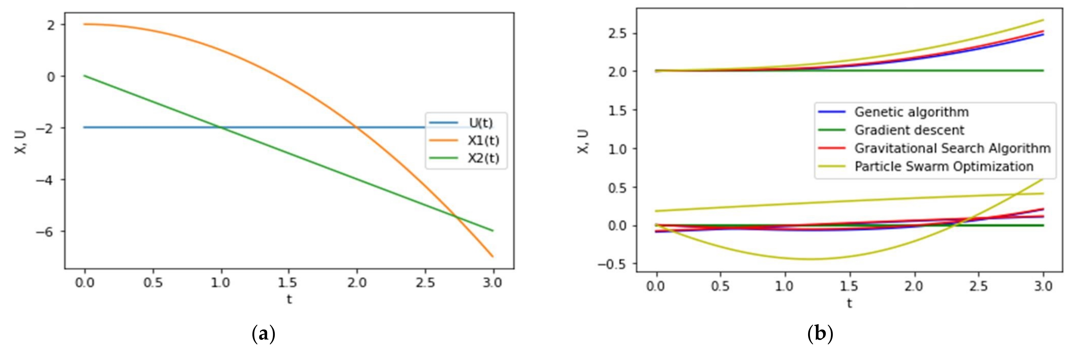
Example 2. Stuck algorithms at the local optimum.
In order to check how an increase in the dimension of the optimal control problem affects the convergence and accuracy of the resulting solution, we investigate the following problem. Consider a two-dimensional problem with respect to the trajectory of optimal control with mixed constraints of the form:
The corresponding optimization problem (26) has the form:
where
and
Figure 8 shows neural network solutions obtained using various optimization methods. The calculated values of the additive error of the optimal pair of neural network approximation are presented in
Table 5.
An increase in the dimensionality in this OCP along the phase trajectory and conjugate variables led to the fact that the considered evolutionary algorithms, as well as the gradient descent algorithm, fell into the local optimum of the minimized function.
5. Conclusions and Future Work
An analysis of the application of various optimization algorithms for neural network solution of optimal control problems showed that evolutionary function optimization algorithms use the least number of iterations to achieve a given accuracy, but finding the exact global minimum is difficult and requires significant computing resources;
Multi-agent methods of gravity search and swarm of particles show the longest execution time for iteration. For quadratic optimal control problems, as well as for linear ones, the genetic optimization algorithm showed the fastest rate of convergence relative to the total execution time of the algorithm. However, for linear optimal control problems, the number of iterations required to achieve the specified accuracy was approximately two times less.
Among evolutionary algorithms, the basic algorithm for optimizing a swarm of particles turned out to be less resistant to hitting a local optimum. The results obtained can be explained by the disadvantage of the PSO algorithm in the absence of procedures for exiting local optima, as well as by the complexity of the selection of the algorithm parameters. In addition, the algorithm of gravitational search and swarm of particles, when implemented, requires lengthy computations of iteration due to the need to recalculate many parameters.
Following from this research, it is planned to study a wider range of multi-agent optimization methods and genetic algorithms, their various modifications, and also to apply the results obtained in the framework of solving applied problems in various scientific fields.


