Abstract
Robots have poor adaptive ability in terms of formation control and obstacle avoidance control in unknown complex environments. To address this problem, in this paper, we propose a new motion planning method based on flocking control and reinforcement learning. It uses flocking control to implement a multi-robot orderly motion. To avoid the trap of potential fields faced during flocking control, the flocking control is optimized, and the strategy of wall-following behavior control is designed. In this paper, reinforcement learning is adopted to implement the robotic behavioral decision and to enhance the analytical and predictive abilities of the robot during motion planning in an unknown environment. A visual simulation platform is developed in this paper, on which researchers can test algorithms for multi-robot motion control, such as obstacle avoidance control, formation control, path planning and reinforcement learning strategy. As shown by the simulation experiments, the motion planning method presented in this paper can enhance the abilities of multi-robot systems to self-learn and self-adapt under a fully unknown environment with complex obstacles.
1. Introduction
A mobile robot is a complex system which must integrate different aspects of environmental perception, motion planning, dynamic decision-making, behavior control and execution. Mobile robots have been widely applied to the management of industrial and agricultural applications, space and ocean exploration, environment monitoring, disaster relief, and national defense. Multi-robot systems consist of multiple individual robots which collaborate to accomplish complex tasks which may be impossible for a single robot to complete. The contemporary study of multi-robot systems has revealed several engineering and technological issues. Research of multi-robot formation control is one of the key techniques in multi-robot cooperation and coordination. Robots are required to form or change specific shapes of formation in some specific application tasks, such as cooperative exploration, obstacle avoidance and transportation planning. Many scholars have studied the formation control of multi-mobile robots, and the main contents of formation control can be summarized as formation generation, formation stability, formation switching, system obstacle avoidance and formation adaptive [1,2,3,4,5,6]. Obstacle avoidance control is another key technique due to the difficulty that each robot in the system needs to securely bypass the various obstacles to reach their destination or goal node [7,8]. Mobile robots have many applications in logistics, including warehousing and delivery, where both machine learning and operations research techniques are applied [9,10]. There are two types of motion planning: (i) global path planning using fully known environmental information; and (ii) local motion planning using fully unknown or partially unknown environmental information. Many effective solutions have been presented to address the obstacle avoidance problem under known environmental conditions. Commonly proposed solutions are the artificial potential field, grid method, visibility graph method and free-space method. Compared with the fully known environment, it is more difficult for robots to avoid obstacles under a fully unknown environment or an environment with complex obstacles. We study the optimal method of formation control and obstacle avoidance control in an unknown multi-obstacle environment for multiple mobile robots.
However, in a multi-robot flocking motion system, it is easy to lead to a potential field “trap”. This can occur if the number of robots and the obstacle intensity degree increases, or the obstacle motion environment is complex. If the robots obtain all information of the environment, they can use motion planning to avoid the areas where the potential field “trap” may occur. However, the motion planning of a robot, at any time, totally depends on the given overall environmental information. If the environment changes, this information must be collected by all the robots, requiring an extremely large volume of communication between the robots. In view of tackling a dynamic multi-obstacle environment, a robot must quickly solve the “trap” problem, with little local environmental information. Therefore, in this paper, we study how to increase the decision control to make the robot use appropriate obstacle avoidance behavior when facing complex obstacles. For example, during motion in a concave shaped environment with obstacles, depending on only two behaviors, obstacle avoidance and moving toward the target may not be optimal. It may lead to oscillation or dead-loop of the robot, or even motion stopping, which may make the robot enter a deadlock state, preventing the robot from reaching the target.
In this paper, it is determined that a robot needs to generate a series of behaviors before reaching the target. Its basic behaviors include running toward the target, obstacle avoidance, collision avoidance, and wall-following motion. It is very important to select the appropriate behavior in the light of the environment. Merely relying on the designer’s experience and knowledge may make it hard for the multi-robot system to adapt to complex and uncertain environments. In order to make the capabilities of the robot’s behavior selection flexible and effective, the robot must have specific abilities to recognize, judge, compare, and self-adjust while interacting with the environment. Therefore, a learning mechanism is introduced to enable motion planning for robots in this paper. Reinforcement learning, an important type of machine learning, can be used to build an interactive relationship between the robot and the complex and dynamic environment.
The application area of our work is a logistics robot. The working environment of a robot may be complicated with multiple obstacles; hence, the robot needs the ability to effectively avoid all the obstacles. Multiple robots need to work together to realize the formation control. The working environment may comprise narrow passages, and the robots are supposed to possess the ability to promptly change their formation. Logistics robots often work in a fixed environment; hence, they must have the potential to explore and memorize the working environment and adopt the optimal strategy. After learning, the robots must become familiar with the routes and plan the next move quickly and effectively.
Our research focuses on the following three aspects:
(1) An advanced multi-robot motion planning system based on flocking control and reinforcement learning is proposed in this paper. This flocking control makes the robot produce the behavior of running to the target, avoiding the obstacle, and formation control. Reinforcement learning enables the robots to learn the environment and select appropriate behaviors and actions for the flocking movement;
(2) The robot can only obtain the local environmental information in the dynamic environment. Nonetheless, it needs to quickly solve the problem where the traditional cluster control falls into the potential field “trap”. To address this issue, this paper presents the optimization algorithm of flocking motion. A hybrid algorithm based on flocking control and reinforcement learning is designed, which can reduce trial and error, thereby improving the learning efficiency in the exploration stage;
(3) The proposed algorithm is simulated and experimented, taking several aspects into consideration. Obstacle-avoidance and formation control effects of the flocking control optimization algorithm proposed in the paper are preliminarily tested in the MATLAB simulation environment. A visual simulation platform has been developed to test the proposed algorithm, which can not only observe the movement of the robots, but also observe the motion planning strategy based on the reinforcement learning and the output value of control quantity of each behavior based on flocking control in real time. The data visualization of process control can thus be realized. Eventually, the proposed algorithm has been transplanted to robot operating system (ROS)-based wheeled robotic vehicles for further experiments.
The paper is organized as follows: related work is introduced in Section 2. In the third section, a block diagram of a multi-robot motion planning system based on flocking control and reinforcement learning is presented, along with the design of the optimization algorithm of flocking control in obstacle avoidance and formation control of robots. In the fourth section, the functional modules of multi-robot motion planning based on reinforcement learning algorithms are designed. The fifth section represents the simulation and experimental results. The conclusion is mentioned in Section 6.
2. Related Work
Among the various motion coordination algorithms, the flocking control mode is a new coordination approach which has been widely accepted and applied to the theoretical study of multi-agent systems. Using this concept of potential field, flocking can unify individual behaviors for formation keeping, running towards a target, and obstacle and collision avoidance, making the process of motion coordination closer to that in the natural world. The accurate quantization of the potential field makes flocking measurable, thus making it possible to calculate a topological formation configuration which can be used to study the stability of flocking. Han [11] explained the three basic rules of flocking behavior: (i) separability; (ii) cohesiveness; and (iii) permutation. All the individual members of a flock can be expressed as agents. Zhao [12] proposed a flocking model based on the velocity matching rule. Yazdani [13] proved that flocking control could achieve a high control effect for multi-robot formation management and path tracking. Hung [14] studied the formation control of a leader-based multi-agent flocking motion. Kumar [15] used the Boid flocking algorithm to generate group position movements. Raj J.A. [16] proposed a set of nonlinear continuous control laws via the Lyapunov-based control scheme for collision, obstacle, and swarm avoidances. Additionally, a leader–follower strategy is utilized to allow the flock to split and rejoin when approaching obstacles. Kumar S. [17] proposed a hybrid approach of intelligent water drop and genetic algorithm technique and executed it in order to obtain global optimal path by replacing local optimal points. Many studies have proved the effectiveness and advantages of flocking control for multi-robot formation, coordination control, and obstacle avoidance control [18,19,20].
Reinforcement learning is a kind of machine learning where an agent maps aspects such as the environmental state and the behavior, to take action to obtain the maximum accumulated reinforcement signals (reward) from the environment. Complicated tasks require robots to possess an ability to self-learn, which is essential to control strategy. This can be used to make the robot realize the automatic mapping between unsupervised information observation and action performance, to save time and cost. There already exist some learning techniques to help a robot self-learn. Reinforcement learning is an important machine learning method. It has been gradually developed ever since Minsky firstly proposed the term “reinforcement learning”. So far, the existing algorithms include the TD(λ) algorithm [21], the Q-Learning, the Sarsa algorithm [22], and the Actor–Chile algorithm [23], among others. Reinforcement learning has been generalized and applied to the field of robotics, such as navigation [24], trajectory tracking [25,26], path planning [27], balance control [28,29], decision-making [30].
These works have proved the effectiveness of flocking control for multi-robot coordination control and the advantages of reinforcement learning for the automatic mapping between unsupervised information observation and action performance. The focus of this paper is on the exploration of a new motion planning method based on flocking control and reinforcement learning in unknown complex environments. To avoid the trap of potential field faced during traditional flocking control, flocking control is optimized. We add reinforcement learning to the behavior-based robot technology. Reinforcement learning enhances a robot’s analytical and predictive ability to select appropriate actions to perform flocking motion.
3. Multi-Robot Motion Planning System Structure
In this paper, flocking control is adopted to ensure that all robots avoid collisions and move together towards a target. Reinforcement learning is used to enhance the robots’ ability to analyze, predict, and select appropriate actions to perform flocking motion. The proposed system combines reinforcement learning in discrete space and flocking control in continuous spaces. This generates an effective combination of high-level behaviors (discrete state and action) and low-level behaviors (continuous state and behavior). As shown in Figure 1, the control system structure includes two main parts: (i) the reinforcement learning module for behavioral strategies; and (ii) the flocking control module for motion planning.
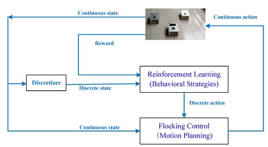
Figure 1.
Multi-robot motion planning system based on flocking control and reinforcement learning.
The system combines behavior-based robot technology and flocking control, to facilitate the mobile robots with an overall behavior to achieve the target. It is important to select the appropriate behavior in light of the environment, and therefore, there is a need to use adaptive machine learning algorithms to make the decisions. Therefore, as shown in Figure 2, the system control structure includes the sensing module, the behavior module, the reinforcement module, the selection module and the execution module.
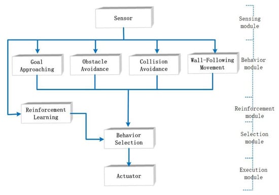
Figure 2.
The control structure of behavior-based robots.
As shown in Figure 3, multi-robot flocking motion includes the principles of moving towards the target point, collision avoidance, obstacle avoidance, and formation control. In this work, we study the optimization design of the flocking motion to further improve the environmental self-adaptability for multiple mobile robots.
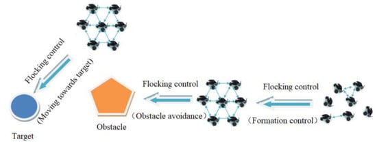
Figure 3.
Multi-robot flocking motion control.
3.1. Multi-Robot Flocking Motion Control
The definition of flocking was presented as [31]:
(1) Separability: each member avoids collisions;
(2) Cohesiveness: each member converges towards an average position;
(3) Permutation: each member moves together in the same direction.
In a flock containing n agents, the dynamics equation of the agent is:
where is the position vector of the agent i, is the velocity vector of the agent i, and is the accelerated velocity vector of the agent i (control input), where is the control vector to balance the velocity between the agents, and is the control vector to control the distance between the agents.
Flocking motion can be of two types: (i) non-leader-based flocking motion; and (ii) leader-based flocking motion. Compared with non-leader-based flocking motion, leader-based flocking motion can create order in the behavior of the entire flock. In this paper, we study the leader-based flocking motion. To control the behavior of the entire flock, we only need to control the behavior or tracks of the leader. Apart from the leader, all the other agents are called followers. Controlling the motion of the leader simplifies the multi-agent control into the control of the motion of a single robot.
The artificial potential field function is a non-negative, differentiable unbounded function to represent the distance , , and satisfies the following conditions:
- (1)
- When ;
- (2)
- When distance reaches a certain value, reaches its minimum value.
3.2. Leader-Follower Flocking Control Design
When a leader is introduced into the flocking motion, other members will follow the leader to perform the same motion—to create order in the whole flock. In the leader-based flocking control, due to the division of the agents into a leader and followers, the flocking control law needs to be designed accordingly to complete the motion control and perform the obstacle avoidance control.
In a flock, when there is a leader, the velocity vectors of all the follower agents of this flock will gradually approach the velocity vector of the leader.
Let the leader run at a velocity of . Then, in the relative coordinate, taking the leader as the reference point, the position vector of a follower relative to the leader can be expressed as ; its velocity vector can be expressed as ; and the distance between the follower and any agent can be expressed as , and .
Then, the total artificial potential field function of a follower can be written as:
where Nl is the adjacent set of the leader.
By further deduction, for the leader, its control law is:
The motion of a robot in an environment is regarded as being under an artificial force field. An obstacle produces a force of repulsion for the robot, while the target point produces a force of attraction to the robot. The resultant force of the attraction and the repulsion is taken as the accelerating force of the robot which can be used to control the motion of the robot. It is generally used for obstacle avoidance control.
The frequently-used attraction function is:
where is the attraction coefficient, and refers to the distance of the object’s present state and the target.
According to the derivative of the attraction field, the attraction can be written as:
However, this attraction function suffers from some defects, because it may lead to collisions with obstacles. In order to avoid colliding with an obstacle due to the large force of attraction caused by being far from the target point, the attraction function is revised as:
According to a derivative of the attraction field, the attraction can be written as:
where refers to the distance between the robot’s present state and the target, and provides a threshold and sets a limit to the distance between the target and the object.
The traditional repulsive function can be written as:
where is the coefficient of repulsion, and refers to the distance between the robot’s present state and the obstacle.
According to a derivative of the repulsion field, the repulsion is:
After adding the effects of the distance between the target and object, and performing some optimization, the corresponding repulsive function becomes:
According to a derivative of the repulsion field, the repulsion is:
where
In this paper, the designed controller for tending towards the target produces an attraction according to Equation (8), and the obstacle avoidance controller produces the repulsion according to Equation (12).
The potential field energy of the interaction among the multiple robots in the system is called the internal potential energy . The potential field energy of the interaction between a single robot with the external environment is called the external potential energy . This includes the repulsion potential energy from the obstacle and the attraction potential energy from the target.
For , we have:
where is the adjustment coefficient of the potential field with , and is the construction coefficient with .
For , we have:
In Equations (20) and (21), is the distance between the robot and the obstacle. For , we have:
In Equations (19) and (20), is the distance between the robot and the target.
When performing obstacle avoidance control in the non-leader-based multi-robot scenario, ; while when performing obstacle avoidance control in the leader-based multi-robot scenario, .
Followers are regarded as obstacles. The repulsion potential field of obstacles is directly applied to keep a considerable distance between robots and effectively prevent collisions. According to different network topology structures that need to be formed in the formation task, such as line, triangular, diamond, the follower has to constantly correct its position relative to the leader. The force analysis diagram is shown in Figure 4.
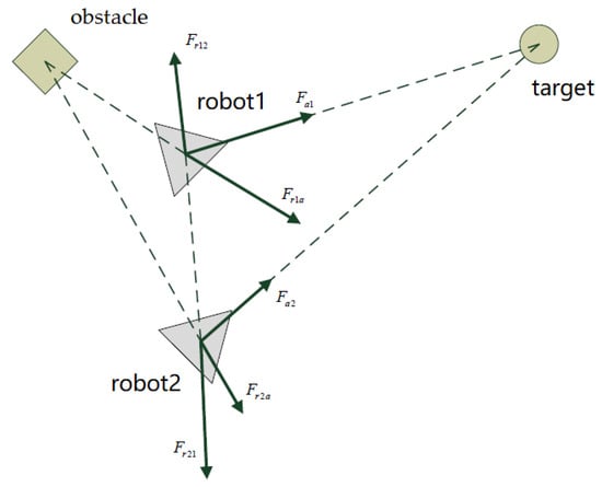
Figure 4.
The force analysis diagram.
In each time period, the direction of motion and next step size of a robot should be calculated, which then obtains the total direction and step size, so as to obtain the position of the robot after the end of the cycle.
3.3. Formation Change
Multi-robot swarms are vulnerable to disturbances that prevent them from maintaining their formation, which can cause followers to lose their leader and the formation to be completely destroyed. In order to better cope with the actual application of emergency, the flocking control algorithm needs to be further optimized. If the leader suddenly receives a huge repulsion from both sides of the forward direction, or if one of the robots in the crowd receives a huge repulsion from one direction or another, the formation (such as diamond formation) needs to be transformed into a kind of safer formation (such as line formation). When the robots are completely out of the dangerous environment, they will return to their original formation.
Formation changing algorithms consist of a sensor module and the execution module, as below:
Step 1: The robots keep a formation and move toward the target based on flocking control designed;
Step 2: The system judges whether the condition of formation change is satisfied according to the distance between each robot and the nearest obstacle. For example, when the repulsion force on both sides of the forward direction of the leader robot exceeds the threshold, it indicates a narrow obstacle ahead, then robots need to change formation;
Step 3: When the condition of formation change is satisfied, robots change into line formation;
Step 4: The robots move forward in line formation until each robot reaches a safe distance from the obstacle;
Step 5: The robots change into the original formation.
3.4. Wall-Following Motion Control
Under some complex environments with obstacles such as concave shape obstacles, the potential field can easily fall into a locally optimal solution or an oscillation point. If the system merely relies on the behaviors of obstacle avoidance and running towards the target, the robot may not reach the target point. After introducing the wall-following motion, even though the robot only knows the local environmental information, it can quickly solve the local tiny problems to reach the target point.
The manifestation of the behavior of wall-following motion is the act of actually moving along the edge of the obstacle. The “wall surface” generally means the outline of an object, which is detected by the laser beam produced by the laser range finder carried in the front of the robot. As shown in Figure 5, judging the trend of the wall is performed using the average filtering method.
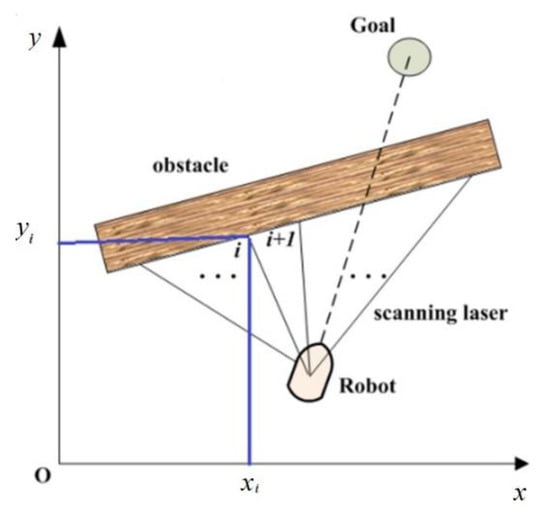
Figure 5.
Multi-robot flocking motion control.
In Figure 5, the coordinate of the wall surface point scanned by the laser is , and the angle formed by the vector lines between the laser point i and i+1 is:
For the trend of the wall surface, (N ≥ 2) is the number of the laser points reflected back. When N = 1, the robot maintains the same direction and continues moving. When N ≥ 2 and the included angle between the direction of the wall and robot is greater than 90°, the robot will turn back and conduct wall-following motion in the opposite direction.
The algorithm has the following five steps:
Step 1: Estimate the condition of the wall-following behavior.
During the process of using the potential field to perform obstacle avoidance motion, the robots enter into a potential field “trap” and then into a deadlock state. At this moment, the robots will produce a certain oscillation and may even stop moving. When checking if the robots are in a deadlock state, the system estimates that the current state satisfies the condition of the wall-following behavior.
Step 2: Flocking-ordered motion turning into wall-following motion.
When the leader robot’s current state satisfies the condition of the wall-following behavior, it breaks away from the flocking ordered motion, and enters into the state of the wall-following motion.
Step 3: Wall-following motion.
When the leader enters into the state of wall-following motion, it will determine the direction of the wall surface according to the modeling method of the “wall surface”. The robots change into line formation. The leader moves at a constant velocity along the direction of the wall surface and the followers follow it. They check the distance between the wall surface obstacle and the leader. When there is a force of repulsion between the wall surface obstacle and the leader robot, the robot will maintain a safe distance from the wall surface, while wall-following. Similar to the obstacle avoidance controller, the wall-following controller also exerts a force on the robot to make it move.
Step 4: Estimate the end condition of the wall-following behavior.
When the leader robot conducts wall-following motion, it will continuously estimate the disappearing condition of the wall surface. If it satisfies either of the two disappearing conditions, the robots will change into the flocking ordered motion. The conditions to estimate the end of wall-following motion are: (i) in the process of obstacle avoidance, when a substantive robot cannot detect any obstacle in the detectable range, the wall-following behavior ends; (ii) when the angle between the repulsion direction of the wall surface against a robot and the attraction direction of target point against the substantive robot is an acute angle, although the robot can still check out the obstacle, it will leave the wall surface and move towards the target point. This is because both the attraction of the target point and the repulsion from the walls force the physical robot to move toward the target point.
Step 5: Wall-following motion changing into flocking ordered motion.
Once the wall-following motion ends, the robot will join back into the multi-robot system to perform flocking ordered motion. In this process, when the robot enters back into the flock, the algorithm is switched to collision avoidance control, and the robot will keep a safe distance from other robots.
4. Reinforcement Learning Algorithm for Behavior-Based Robots
The behavior-based multi-robot system gains the local environment information in real time and performs the actions of moving towards the target, avoiding obstacles, and performing wall-following motion to complete the motion planning. In this paper, reinforcement learning is added into the multi-robot flocking motion, to improve the robot’s analytical and predictive abilities to select appropriate behaviors to perform flocking motion. Reinforcement learning has the advantage of being independent from the environment model and leads to a highly robust system. This helps to add the behavior-based robot technology into flocking control to make the robot generate behaviors.
Reinforcement learning is used to solve the problems of how to make agents use learning strategies to maximize rewards during interaction with the environment.
In Figure 6, the agent is the subject of learning and decision making. Environment refers to the external world recognized by the agent and interacts with the agent. The reward is information indicates whether an agent has performed good or bad behavior. In this paper, reinforcement learning is applied to robot motion planning, as shown in Figure 7.
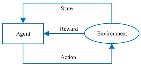
Figure 6.
Construction of reinforcement learning.
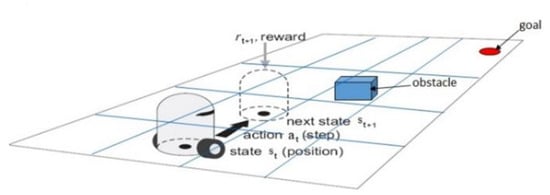
Figure 7.
Robot motion planning based on reinforcement learning.
The external environment merely provides limited local information; therefore, a reinforcement learning-based system must rely on its own experiences to learn, and then improve its motion plan. In this paper, the Q-learning algorithm is adopted.
The value function of reinforcement learning is:
where is called the accumulated returns of conversion obtained from the initial state s using the strategy .
During each iteration of learning, the agent needs not only to consider the state but also the action. Q function is obtained as:
where is the selected action at time from the action set . The purpose of the system is to maximize the total bonus value, so is used to replace the in the equation, and a new equation is obtained as:
At time , the agent chooses an action according to the current state, and then updates the new Q value by the following equation:
where is the selected action at state .
Q-learning converges under the following convergence conditions [32,33]:
- (1)
- Environment is the Markov process;
- (2)
- Lookup is used to represent the Q function;
- (3)
- Each state–action pair can be repeated in the experiments unlimited times;
- (4)
- The right selection of learning rate is required.
When the given bounded reinforcement signal is and the learning rate is
and , then is convergent to the optimal with learning rate .
Motion control based on the Q-learning algorithm includes a reinforcement module and an action selection module. The role of the reinforcement module is to provide a reinforcement signal for the action selection module. The flowchart of the reinforcement module is:
The reinforcement signal returned by the reinforcement module is of two types: one is used to compare the distance between the robot and the target at the current time with what it was at a previous time; another is used to compare the distance between the robot and obstacle with what it was at a previous time, and fusing these two kinds of signals.
For the comparison of the distance between the robot and the target at the current time what it was at a previous time, the following bonus-penalty is used:
For the comparison of the distance between the robot and obstacle at the current time and what it was at a previous time, the following bonus-penalty is used:
To explore all the possible actions, at the initial stage, the Boltzmann distribution is used to perform the random selection of actions. According to the Boltzmann distribution, the probability of an action being selected is:
In Equation (29), T is the virtual problem, and with an increase in T, the randomness of the selection becomes stronger.
As the learning progresses, the Q value will tend towards the desired value, and hence it is not appropriate to use a randomness algorithm to select actions. Therefore, at this time, the corresponding action of the maximum Q value at the current state is chosen according to a greedy strategy.
The action selection module is designed and implemented by combining the learning time, the Boltzmann distribution, and the greedy strategy.
With the increase in the learning time, the corresponding probability value and the time to adopt the greedy strategy will also increase. Greedy strategy selects the motion with a maximum Q value of the corresponding action based on the input state, and returns the index number of the Q value array for this action in the corresponding state.
The reinforcement learning algorithm for behavior-based robots is as below:
Step 1: Obtain the robot’s current state;
Step 2: Obtain a random value;
Step 3: Select actions based on the random values using Boltzmann distributions or greedy strategies;
Step 4: Execute this action;
Step 5: Obtain a new state;
Step 6: Input the new state into the reinforcement module to obtain the reinforcement signal;
Step 7: Update the Q value according to the reinforcement signal and Equation (26).
5. Simulation
The algorithm proposed in this paper was simulated in MATLAB, and a visual simulation platform for multi-robot motion planning was also developed to verify the designed algorithms more intuitively.
5.1. MATLAB Simulation
We used MATLAB to simulate the obstacle avoidance control and formation transformation algorithm proposed in this paper for multiple robots in a complex obstacle environment. We also designed a simulation interface, which can be customized by the user to set up obstacle environment and robot settings.
We designed a simulation interface for multi-robot formation control in MATLAB, as shown in Figure 8a. The user can customize the obstacle scene and robot settings. Simulation results show that the pilot robot and the following robot form a diamond formation and move towards the target position. If the robots detect obstacles with a narrow passage, then they change formation and form a straight line. After moving through the barrier, the robots change formation back to a diamond formation again. When the robots reach the target point, they turn into a line formation.
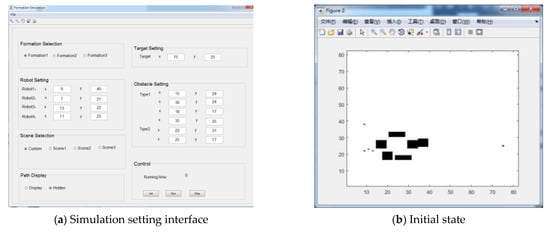
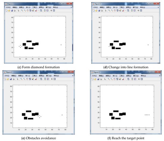
Figure 8.
Motion control in complex obstacles.
5.2. Design and Experiments of the Visual Simulation Platform
In this paper, a visual simulation platform for multi-robot motion planning has been developed to verify the proposed algorithms. Users can freely set robots and obstacles in the simulation platform. There are not only static obstacles but also dynamic moving objects with unpredictable behaviors. The traditional motion planning approaches are often designed based on static, known maps, and while facing emergency situations, the robot is vulnerable to bump into an obstacle, which leads to a high damage rate of the robots, causing unnecessary economic losses. The three-dimensional simulation platform has intuitive advantages than a traditional two-dimensional plane. The simulation scenario is closer to the real environment, exhibiting the overall motion planning situations, which makes data three-dimensional and comprehensive.
We utilized the Visual Studio Community software and Unity3D engine to develop the simulation system. The simulation platform is divided into three modules: the interface module, the algorithm module, and the robot module.
The functions of the simulation system are generally divided into eight aspects. These are scene modeling, robot setup, formation control, obstacle avoidance control, learning training, path planning, switching windows, and system options.
- (1)
- Scene modeling: The users can simulate the real environment to establish a virtual environment. They can set up the obstacles, change the locations of obstacles, add or delete obstacles, and freely set up the scenes. They can also configure irregular movements for obstacles in the scene and set up a dynamic obstacle environment;
- (2)
- Robot settings: Users can set the position of robots and the number of robots;
- (3)
- Formation control: The system can perform visualized simulations towards the formation control algorithm designed by the user. The modes of formation control can be divided into those with Leader control and those without Leader control;
- (4)
- Obstacle avoidance control: The system can perform visualized simulations on the algorithm of obstacle avoidance control designed by the user. All the paths that the robots have been running through in the scene can be viewed in real time;
- (5)
- Learning training: The system can perform visualized simulations towards the reinforcement learning algorithm designed by the user. The user can observe the data in the learning process and the running state of robots in real-time. The system stores and reads the data obtained from the training;
- (6)
- Path planning: The system can perform visualized simulations towards the path planning algorithm designed by the users. The robots in the scene perform movement according to the path generated by the algorithm of path planning. The user can observe the movement path of robots;
- (7)
- Switch of the visual window: The user can freely switch the display between data in Q-tables and the current movement scenes of a robot;
- (8)
- System options: The user can configure the simulations and operations through the system options.
The visualized simulation platform interface of multi-robot movement planning is depicted in Figure 9. The right visual window is the real-time tracking of movement situations on robots. The upper-left window of the interface is a three-dimensional visual window of the entire scene. The middle-left window is the setting and control buttons which allow users to configure the simulations. The bottom-left window can view the data of the Q table. We can check the real-time data of the Q-learning process, including the robot status and the three control output values (goal approaching force, obstacle avoidance force, along wall force). The Q-table finally records the best behavior corresponding to each state.
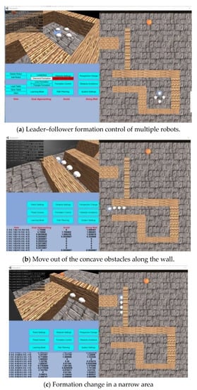
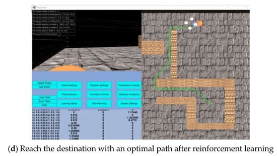
Figure 9.
The visual simulation platform interface of multi-robot motion planning in a complex obstacle environment.
To verify the algorithm designed in this paper, we first set up the obstacle scene and the robots, and then perform verifications via the visualized simulations on the designed algorithm. Figure 9b,c, as seen below, indicate that after the learning training, the robots under the designed control algorithm can perform very well in avoiding obstacles and changing formation when passing through the narrow obstacles. They can also move out of the concave obstacles through their movements along the wall. For a dynamically unknown environment, the motion control enables the robot to effectively avoid obstacles. For a static environment which has been learned, reinforcement learning enables the motion planning of a robot to acquire an optimal path.
5.3. Simulation Analysis
The visual simulation platform is considered a convenient method to set up virtual scenes for actual scenes and to visually observe the control situation of each state, which is considered conducive for the optimization of the proposed control algorithm and simulation comparison.
5.3.1. Simulation Analysis of Obstacle Avoidance and Formation Control Based on Flocking Control
Some important parameters as shown in Table 1, such as the attraction coefficient ε in Equations (5) and (6), the coefficient of repulsion η in Equation (9), and the adjustment coefficient of the potential field A in Equation (15) of the flocking control algorithm affecting the control effect. The hyperparameter ε is a gain coefficient for the attraction field and attraction force (the negative gradient of the attraction field). The hyperparameter η is a gain coefficient for the repulsion field and repulsion force (the negative gradient of the repulsion field). The hyperparameter A is a gain coefficient of the internal potential field energy of the interaction among the multiple robots.

Table 1.
Descriptions of flocking control hyperparameters
We debug these parameters by simulation as discussed below.
- (a)
- Set η = 0.2~0.6, ε = 1, η/ε = 0.2~0.6, A = 1~2,
For both static and dynamic obstacles, the robot can avoid obstacles. The robot cannot remain steady during formation. The formation changes very slowly when it encounters obstacles.
- (b)
- Set η = 0.7~1, ε = 1, η/ε = 0.7~1, A = 3~4,
The robot can avoid the static obstacles, but it cannot react quickly to the dynamic obstacles that appear suddenly. The formation can be basically maintained when there are no obstacles, but it cannot be changed in time when there are obstacles.
- (c)
- Set η = 1~1.5, ε = 1, η/ε = 1~1.5, A = 4~6,
The robot can avoid both static and dynamic obstacles, maintain the formation stably when there are no obstacles, and change the formation in time when there are obstacles.
- (d)
- Set η = 1.5~2, ε = 1, η/ε = 1.5~2, A = 7~9,
For static and dynamic obstacles, the robot can avoid obstacles and move to a relatively longer distance, with a slightly longer avoidance path. The formation can be basically maintained, but it is a little unsteady. Sometimes, the robot deviates from the formation position. When robots encounter obstacles, the formation transformation is not considered ideal, and they often deviate from the team.
By using the simulation platform to simulate various situations, it is found that η/ε displays a significant influence on the obstacle avoidance effect of the robot. When η/ε is less than 1, the robot cannot achieve effective obstacle avoidance. When η/ε is greater than 1, the robot can basically avoid obstacles. However, with an increase in the value of η/ε, the robot can avoid obstacles quite early, and the avoidance path can become longer. The obstacle avoidance effect of η/ε shows better control between 1.0 and 1.5. The adjustment coefficient of the potential field A shows certain influence on the reaction speed of the formation control when the formation changes. The potential field A shows a good formation control effect between 4 and 6. We study the influence of these hyperparameters on the control, which is helpful for us to quickly adjust hyperparameters according to the actual application to achieve a better control effect.
5.3.2. Simulation Comparison between Traditional Flocking Control and Flocking Control with the Wall-Following Strategy in a Complex Obstacle Environment
The potential field “trap” commonly occurs when a concave-shaped obstacle is used. The avoiding obstacles and those moving toward the target cause the robot to oscillate or loop, or even stop its movement and enter the deadlock state so that the robot cannot move out of the dead zone, as shown in Figure 10a. The obstacle avoidance control strategy is designed based on wall-following behavior and generates the control force for moving the robot along the boundary of the obstacle and getting out of the trap, as shown in Figure 10b. The optimized obstacle avoidance control algorithm can enhance the robot’s adaptive ability in a complex obstacle environment.
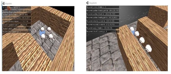
Figure 10.
Simulation comparison of the obstacle avoidance control under a concave-shape obstacle environment.
5.3.3. Simulation Comparison between Reinforcement Learning and Hybrid Algorithm in an Unknown Dynamic Environment
Some path planning methods need global information. In an unknown environment, these methods are not applicable. The reinforcement learning method is considered helpful in exploring the environment by using a random strategy. However, random attempts take more time in exploring many unnecessary states, which thus reduce the learning efficiency. Therefore, we need to pay attention to both exploration and the exploitation of strategy.
Therefore, the proposed hybrid algorithm in this paper introduces the potential field of flocking control in the reinforcement learning training stage, and the robot becomes attracted to the target to reduce the number of trials. The flocking control has no memory and learning ability, whereas reinforcement learning can remember the control of each state experienced and can continuously learn to choose the optimal control.
In order to compare the performance of the traditional reinforcement learning and the hybrid algorithm, we designed a complex obstacle environment on the simulation platform and added moving obstacles. The convergence simulation of the training process of the two algorithms is shown in Figure 11.
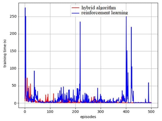
Figure 11.
Simulation comparison of the training process in an unknown dynamic environment.
The goal of the traditional reinforcement learning method is to obtain an optimal strategy, which is to maximize the cumulative reward obtained by the robot action sequence. This suggests that the action with the largest value function must be selected in each state. However, at the early stage of training, the value function could not reach the optimal state, so the action selected by maximizing the Q value was not optimal. Hence, there must be a certain probability to randomly select actions to explore the optimal strategy. The -greedy action selection strategy has been adopted here to explore the optimal strategy and avoid falling into the local optimal solution, wherein the actions are randomly selected in the action space for exploration by probability , and the optimal action under the current knowledge is selected by probability 1− . The abnormal disturbance observed in Figure 11 is due to the bad strategy caused by the randomly selected actions. When the robot is exploring with probability, the training time is very long due to the bad strategy, and the curve exhibits fluctuation disturbance. Reinforcement learning exploration is accompanied by randomness; therefore, it is not a smooth downward curve as in normal supervised learning. The system curve tends to fluctuate frequently.
As shown in Figure 11, in the training stage, the hybrid algorithm with flocking control can reduce the trial and error and improve the learning efficiency in the exploration stage as compared to the traditional reinforcement learning. Moving obstacles make the training of reinforcement learning not converge well, and there can be significant fluctuation. The hybrid algorithm can converge faster and is more stable, which significantly reduces the training time.
For reinforcement learning, the discounting factor γ and the learning rate α in Equation (26) are considered important parameters, as shown in Table 2. The parameter γ denotes the degree of emphasis put on future rewards. After simulation debugging, we found that when γ = 0.1–0.5, irrespective of the learning rate, the algorithm could not be successfully trained, and the training time was very long. When γ > 0.5, algorithm training accelerated. After testing, we set γ = 0.9 and ensured that the training was relatively fast, but it did not lead to non-convergent variance. The greater the learning rate α, the less the effect of the previous training, and the Q table will be updated in the best possible way with each update so that the convergence speed will be faster. After debugging, we set α = 0.9–1, and it required fewer trained episodes to correctly update the Q table and find the best policy.
Table 2.
Descriptions of reinforcement learning hyperparameters.
A display interface is designed on the visualization platform for behavior-based robots as shown Figure 12. The “Learning Mode” button can show the potential field forces, e.g., state, goal avoidance force, obstacle avoidance force, and along the wall force, of the robot in the training phase. The robot can first explore the unknown environment and save the data in the Q table of reinforcement learning. If robots move in the same environment in the future, they can directly avoid obstacles and approach the target very quickly because they have acquired and learned the best motion planning decision. When encountering a concave obstacle, the behavior along the wall can be recorded by reinforcement learning, avoiding the repeating exploration path, and calculating the control force.
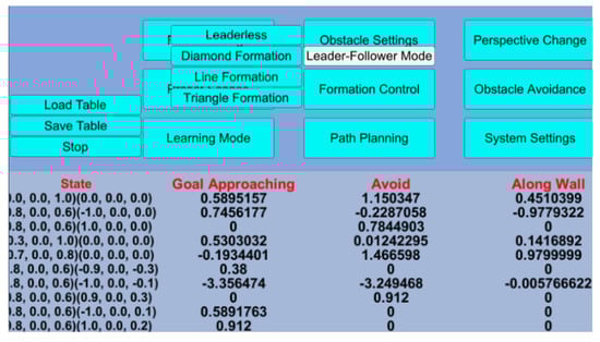
Figure 12.
A display interface designed on the visualization platform for behavior-based robots.
In summary, we have compared the performance of the traditional flocking control, optimized flocking control with the wall-following strategy, traditional reinforcement learning and the hybrid algorithm-based optimized flocking control and reinforcement learning for multi-robot motion planning in a complex obstacle environment. The simulation result shows that the hybrid algorithm is better than others. The performance comparison of algorithms is shown in Table 3.
Table 3.
Performance comparison of algorithms.
6. Mobile Robot Experiments
In this section, three mobile robot HITM-based robot operating systems (ROSs) are utilized to validate the stability, convergence, and robustness of the algorithm. Based on the proposed algorithm, different kinds of experiments are conducted.
We transplanted the control algorithm written in Python code on the visual simulation platform to the ROS system of the mobile robot, and firstly tested in the ROS simulation as shown in Figure 13.
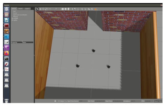
Figure 13.
Robot operating system (ROS) simulation for multi-robot motion planning.
In the experiments, the robot followed the stabilized formation. The effective communication range was estimated to be 500 m. The mobile robot HITM as composed of many modules, such as an on-board upper computer, laser radar, and RF modules. The upper computer as the ROS host conducted information interactions with the ROS slave on the client PC by routing and networking through wireless Wi-Fi signals. The main control panel could also interact with the client embedded development board by using the RF module in the form of 2.4G wireless communication.
ROS is a distributed software framework in which nodes can run on different computing platforms and communicate by using topics and services. In the multi-machine system, ROS Master can be set to run on a machine car, and other machines can contact the ROS Master by SSH as a slave. In our experiment, three mobile robots were used to test the proposed control algorithm. We carried out the distributed multi-machine communication design for the three mobile robots.
Figure 14 shows that the mobile robots formed a triangular formation and moved toward the target. When the robots encountered a narrow obstacle channel, they changed their formation into a line formation in order to pass through the obstacle. The proposed control algorithm exhibited good control effects.
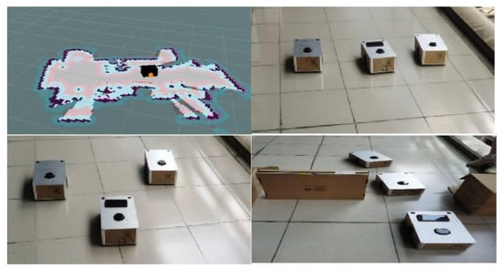
Figure 14.
Motion planning experiments.
7. Conclusions
In this paper, we proposed a kind of novel multi-robot motion planning method based on flocking control and reinforcement learning. Flocking control is adopted to ensure that all robots avoid collisions, control formation, and move together towards a target. Reinforcement learning is used to enhance the robots’ ability to analyze, predict, and select appropriate actions to perform flocking motion.
Under a complex multi-obstacle environment, the problem of oscillation or dead-loop may occur in a multi-robot flocking motion system. Moreover, multi-robot swarms are vulnerable to disturbances that prevent them from maintaining their formation. In this paper, we study how to increase the decision control to make the robot use the appropriate obstacle avoidance behavior when facing complex obstacles. We proposed the optimal design of flocking control. Simulation results show that robots can quickly solve the “trap” problems by wall-following motion and formation change, with little local environmental information.
Robots need to generate a series of behaviors before reaching the target. In order to make the capabilities of the robot’s behavior selection flexible and effective, we added reinforcement learning to the behavior-based robot technology. We design the Q-learning algorithm for multi-robot motion planning in this paper. Simulation results showed that the Q-table records the best behavior corresponding to each state. After learning, the robots directly go straight to the target with optimal motion planning.
Moreover, we developed a visual simulation platform for multi-robot motion planning to verify the proposed algorithms. The interface is intuitive, and vivid robot movements are very convenient for researchers to debug.
Author Contributions
Conceptualization, M.W. and B.Z.; methodology, M.W.; software, M.W. and Q.W.; validation, M.W.;writing—original draft preparation, M.W.; writing—review and editing, B.Z.; visualization, Q.W. All authors have read and agreed to the published version of the manuscript.
Funding
This research was funded by the Natural Science Foundation of Guangdong Province China, grant number 2018A030313868.
Institutional Review Board Statement
Not applicable.
Informed Consent Statement
Not applicable.
Data Availability Statement
The data presented in this study are available on request from the corresponding author.
Conflicts of Interest
The authors declare no conflict of interest.
References
- Dong, C.Y.; Zhang, W.Q.; Wang, Q. Time-varying anti-disturbance formation control for high-order non-linear multi-agent systems with switching directed topologies. IET Contr. Theory Appl. 2020, 14, 271–282. [Google Scholar] [CrossRef]
- Tsai, C.C.; Yu, C.C.; Wu, C.W. Adaptive distributed BLS-FONTSM formation control for uncertain networking heterogeneous omnidirectional mobile multirobots. J. Chin. Inst. Eng. 2020, 43, 171–185. [Google Scholar] [CrossRef]
- Yu, H.J.; Shi, P.; Lim, C.C. Formation control for multi-robot systems with collision avoidance. Int. J. Control. 2019, 92, 2223–2234. [Google Scholar] [CrossRef]
- Qian, D.W.; Zhang, G.G.; Chen, G.R.; Wang, J.; Wu, Y. Coordinated Formation Design of Multi-Robot Systems via an Adaptive-Gain Super-Twisting Sliding Mode Method. Appl. Sci. 2019, 9, 4315. [Google Scholar] [CrossRef]
- Yang, N.N.; Li, J.M. Distributed iterative learning coordination control for leader-follower uncertain non-linear multi-agent systems with input saturation. IET Contr. Theory Appl. 2019, 13, 2252–2260. [Google Scholar] [CrossRef]
- Wee, S.G.; Dai, Y.; Kang, T.H.; Lee, S.G. Variable formation control of multiple robots via VRc and formation switching to accommodate large heading changes by leader robot. Adv. Mech. Eng. 2019, 11, 1–12. [Google Scholar] [CrossRef]
- Ahmad, M. Alshorman, Omar Alshorman.Fuzzy-Based Fault-Tolerant Control for Omnidirectional Mobile Robot. Machines 2020, 8, 55. [Google Scholar]
- Mronga, D.; Knobloch, T. A constraint-based approach for human-robot collision avoidance. Adv. Robot. 2020, 34, 265–281. [Google Scholar] [CrossRef]
- Hyeoksoo, L.; Jongpil, J. Mobile Robot Path Optimization Technique Based on Reinforcement Learning Algorithm in Warehouse Environment. Appl. Sci. 2021, 11, 1209. [Google Scholar]
- Baniasadi, P.; Foumani, M.; SmithMiles, K. A transformation technique for the clustered generalized traveling salesman problem with applications to logistics. Eur. J. Oper. Res. 2020, 285, 444–457. [Google Scholar] [CrossRef]
- Han, T.T.; Ge, S.S. Styled-Velocity Flocking of Autonomous Vehicles: A Systematic Design. IEEE Trans. Autom. Control. 2015, 60, 2015–2030. [Google Scholar] [CrossRef]
- Zhao, X.W.; Hu, B.; Guan, Z.H.; Chen, C.Y. Multi-flocking of networked non-holonomic mobile robots with proximity graphs. IET Contr. Theory Appl. 2016, 10, 2093–2099. [Google Scholar] [CrossRef]
- Yazdani, S.; Haeri, M. Flocking of multi-agent systems with multiple second-order uncoupled linear dynamics and virtual leader. IET Contr. Theory Appl. 2016, 10, 853–860. [Google Scholar] [CrossRef]
- Hung, S.M.; Givigi, S.N. A Q-Learning Approach to Flocking with UAVs in a Stochastic Environment. IEEE T. Cybern. 2017, 47, 186–197. [Google Scholar] [CrossRef] [PubMed]
- Kumar, V.; Bergmann, N.W.; Ahmad, I.; Jurdalk, R.; Kusy, B. Cluster-based Position Tracking of Mobile Sensors. In Proceedings of the 2016 IEEE Conference on Wireless Sensors (ICWiSE), Langkawi, Malaysia, 10–12 October 2016; pp. 7–14. [Google Scholar]
- Raj, J.; Raghuwaiya, K.; Sharma, B.; Vanualailai, J. Motion Control of a Flock of 1-Trailer Robots with Swarm Avoidance. Robotica 2021, 1–26. [Google Scholar] [CrossRef]
- Kumar, S.; Parhi, D.; Pandey, K.; Muni, M. Hybrid IWD-GA: An Approach for Path Optimization and Control of Multiple Mobile Robot in Obscure Static and Dynamic Environments. Robotica 2021, 1–28. [Google Scholar] [CrossRef]
- Zheng, H.H.; Panerati, J.; Beltrame, G. An Adversarial Approach to Private Flocking in Mobile Robot Teams. IEEE Rob. Autom. Lett. 2020, 5, 1009–1016. [Google Scholar] [CrossRef]
- Jing, G.S.; Wang, L. Multiagent Flocking With Angle-Based Formation Shape Control. IEEE Trans. Autom. Control. 2020, 65, 817–823. [Google Scholar] [CrossRef]
- Binh, N.T.; Dai, P.D.; Quang, N.H.; Ty, N.T.; Hung, N.M. Flocking control for two-dimensional multiple agents with limited communication ranges. Int. J. Control. 2020. [Google Scholar] [CrossRef]
- Costa, L.V.O.; Aya, C.C.J. Monte Carlo. TD(λ)-methods for the optimal control of discrete-time Markovian jump linear systems. Automatica 2002, 38, 217–225. [Google Scholar] [CrossRef]
- Wang, Y.H.; Li, T.H.S.; Lin, C.J. Backward Q-learning: The combination of Sarsa algorithm and Q-learning. Eng. Appl. Artif. Intell. 2013, 26, 2184–2193. [Google Scholar] [CrossRef]
- Di Castro, D.; Meir, R. A Convergent Online Single Time Scale Actor Critic Algorithm. J. Mach. Learn. Res. 2010, 11, 367410. [Google Scholar]
- Lachekhab, F.; Tadjine, M.; Kesraoui, M. Experimental evaluation of new navigator of mobile robot using fuzzy Q-learning. Int. J. Eng. Syst. Modell. Simul. 2019, 11, 50–59. [Google Scholar]
- Farinaz, A.; Derhami, V.; Fatemeh, J. A new framework for mobile robot trajectory tracking using depth data and learning algorithms. J. Intell. Fuzzy Syst. 2018, 34, 3969–3982. [Google Scholar]
- Wen, S.H.; Hu, X.H. Q-learning trajectory planning based on Takagi-Sugeno fuzzy parallel distributed compensation structure of humanoid manipulator. Int. J. Adv. Robot. Syst. 2019, 16. [Google Scholar] [CrossRef]
- Bae, H.; Kim, G. Multi-Robot Path Planning Method Using Reinforcement Learning. Appl. Sci. 2019, 9, 3057. [Google Scholar] [CrossRef]
- Rahman, M.; Rashid, S.; Hossain, M. Implementation of Q learning and deep Q network for controlling a self balancing robot model. Rob. Biomim. 2018, 5, 1–8. [Google Scholar]
- Xi, A.; Mudiyanselage, T.; Tao, D. Balance Control of a Biped Robot on a Rotating Platform Based on Efficient Reinforcement Learning. IEEE CAA J. Autom. Sin. 2019, 6, 938–951. [Google Scholar] [CrossRef]
- Shi, H.; Lin, Z.Q.; Zhang, S. An adaptive decision-making method with fuzzy Bayesian reinforcement learning for robot soccer. Inf. Sci. 2018, 436, 268–281. [Google Scholar] [CrossRef]
- Saulnier, K.; Saldana, D.; Prorok, A. Resilient Flocking for Mobile Robot Teams. IEEE Rob. Autom. Lett. 2017, 2, 1039–1046. [Google Scholar] [CrossRef]
- Jang, B.; Kim, M.; Harerimana, G. Q-Learning Algorithms: A Comprehensive Classification and Applications. IEEE Access 2019, 7, 653–667. [Google Scholar] [CrossRef]
- Low, E.; Ong, P.; Cheah, K. Solving the optimal path planning of a mobile robot using improved Q-learning. Robot. Auton. Syst. 2019, 115, 143–161. [Google Scholar] [CrossRef]


Publisher’s Note: MDPI stays neutral with regard to jurisdictional claims in published maps and institutional affiliations. |
© 2021 by the authors. Licensee MDPI, Basel, Switzerland. This article is an open access article distributed under the terms and conditions of the Creative Commons Attribution (CC BY) license (http://creativecommons.org/licenses/by/4.0/).