Article

Probabilistic Condition Monitoring of Azimuth Thrusters Based on Acceleration Measurements

1
Control Engineering, Environmental and Chemical Engineering, University of Oulu, P.O. Box 4300, 90014 Oulu, Finland
2
Kongsberg Maritime Finland Oy, P.O. Box 220, 26101 Rauma, Finland
*
Author to whom correspondence should be addressed.
Machines 2021, 9(2), 39; https://doi.org/10.3390/machines9020039
Submission received: 23 December 2020 / Revised: 5 February 2021 / Accepted: 8 February 2021 / Published: 10 February 2021

Abstract

:
Drill ships and offshore rigs use azimuth thrusters for propulsion, maneuvering and steering, attitude control and dynamic positioning activities. The versatile operating modes and the challenging marine environment create demand for flexible and practical condition monitoring solutions onboard. This study introduces a condition monitoring algorithm using acceleration and shaft speed data to detect anomalies that give information on the defects in the driveline components of the thrusters. Statistical features of vibration are predicted with linear regression models and the residuals are then monitored relative to multivariate normal distributions. The method includes an automated shaft speed selection approach that identifies the normal distributed operational areas from the training data based on the residuals. During monitoring, the squared Mahalanobis distance to the identified distributions is calculated in the defined shaft speed ranges, providing information on the thruster condition. The performance of the method was validated based on data from two operating thrusters and compared with reference classifiers. The results suggest that the method could detect changes in the condition of the thrusters during online monitoring. Moreover, it had high accuracy in the bearing condition related binary classification tests. In conclusion, the algorithm has practical properties that exhibit suitability for online application.

1. Introduction

Azimuth thrusters are used for propulsion systems and dynamic positioning (DP) of offshore platforms and vessels. In a drill ship, the thrusters are used to maintain the ship position by counteracting environmental forces, such as wind, waves and current, but also for propulsion in transit from site to site. The environmental forces, the impacts with external objects like ice blocks, propeller operation, the pulsation from prime movers and accessory systems together inflict complex vibrations and stress to the system [1]. Over the long haul, the stress caused by the harsh environment may lead to fatigue, fracture and tribological issues in the system [2,3]. This inflicts damage to gears and bearings, but also other types of issues, such as propeller failures emerge [4].
The measurement technology for the condition monitoring (CM) of the azimuth thrusters must be economically viable, maintenance-free and reliable due to the closed and inaccessible construction. Therefore, the driveline components, such as the rolling element bearings and gears, are commonly monitored with the well-established indirect methods, such as piezoelectric accelerometers or oil condition and wear debris sensors [5].
Although the vibration responses of propulsion shafts are studied regularly based on laboratory experiments and simulations [1,6], the literature on the practical condition monitoring of azimuth thrusters is rare [2,3]. At the same time, the CM methods for wind turbines, which also experience excessive loads and system oscillations, are studied extensively [7], and the technology could provide useful benchmarks for the thruster monitoring as well.
It is still an industry standard to have a human in the loop when analyzing acceleration sensor data from the noisy marine environment. The common cloud-based approach is limited by the slow data transfer over an offshore satellite network, whereas the fully algorithmic approach enables the analysis on the edge, i.e., locally onboard the offshore vessel. On the edge, the size of the data set can be much larger, enabling the use of data-hungry methods. However, it is possible that the future generations of wireless technologies provide more efficient solutions to data transfer.
Currently, a large part of CM approaches that strive for some level of automation utilize the machine learning methodology, such as the classification approach [8,9]. The research in this field is commonly realized with idealized laboratory experiments, where high accuracies can be reached, as was inferred in [9]. There, the models are typically trained with data from a limited number of operational states, and then tested with samples from the same states. On the contrary, industrial machines may operate in a multitude of operational states rather than a few exclusively. The entire operating area may be so wide that the data used for model training include only a part of the operational states that are possible in practice. New data collected from an operating azimuth thruster, for example, may represent a new operational state influenced by various factors, such as the varying shaft speed and steering angle in the thruster, changing vessel speed and other external factors. This variation is a challenge to the models trained with incomplete information on the actual operation of the system. A model fitted accurately based on few scattered operational states may not correctly recognize new samples which are different from the training samples [10]. Furthermore, the relatively low incidence of faults in industrial machines hinders the proper training of classifiers for the practical applications [11,12].
The condition monitoring of azimuth thrusters could be done based on anomaly detection algorithms [3,12,13] that require training data from the typical operation of the system in a condition without failures. The anomaly detection based on squared Mahalanobis distance [14] particularly has gained a broad interest in condition monitoring [13,15] including wind turbine monitoring applications [16,17]. The major motivation for its use originates from the simplicity and computational efficiency, but on the other hand, it has been reported that the lack of normal distribution in training data, correlated input features, inappropriate threshold limits and environmental variability are some major challenging issues and limitations for the practical application of this method [18,19]. Evidently, this generates specific challenges to the selection of input data for the method which is the major issue highlighted in this research study.
The main contribution of this study is the introduction of the probabilistic condition monitoring algorithm for azimuth thrusters with a semi-automated identification procedure. The data selection challenges discussed above are managed by proposing new solutions to the data processing sequence. Firstly, the disturbed samples are rejected in a data quality control based on monitoring specific characteristics of the acquired acceleration signals. Secondly, the normal distributed data for the squared Mahalanobis distance are ensured by a sample selection procedure that includes a check for normal distribution during model identification. There, the shaft speed values in varying ranges are used in linear regression models to predict the values of vibration features and the residuals are then checked in the hypothesis tests. Thirdly, the multicollinearity in the training data is checked, which makes the identification procedure semi-automated, because the user must replace the correlated features.
The online monitoring process in the algorithm is demonstrated based on real data from two azimuth thrusters in an operating drill ship. Both data sets included a period with an undamaged condition followed by evolving defects. The squared Mahalanobis distance is monitored based on single values and their moving median providing information on the thruster condition. Moreover, the selection of threshold limits is studied based on classification tests and the monitoring performance is compared with several classifiers in a binary classification task.
The remainder of the paper is organized as follows. The first part of Section 2 introduces the azimuth thrusters, measurements, monitored components and the data. The second part introduces the condition monitoring algorithm and the third part describes the procedure used for the performance analysis in the classification tests. Section 3 demonstrates the application of the method, compares its diagnostic performance with the classifiers, and discusses the findings and future directions. Finally, Section 4 concludes the study.

2. Materials and Methods

2.1. Azimuth Thruster

Figure 1 shows an illustration of the azimuth thruster and its main parts. The thruster rotates itself 360 degrees around its vertical axis, which provides flexibility and thrust in every direction for the system. The thruster model type in this study is UUC 455 manufactured by Kongsberg Maritime Finland Oy. These heavy-duty L-drive azimuth thrusters are specifically designed for the dynamic positioning operation on offshore rigs and drill ships. They have Maximum Continuous Rating (MCR) 5.2–5.5 MW, input speed up to 720–750 rpm and propeller diameter 4.1 m. An ensemble of several thrusters (six typically) is usually mounted underneath a vessel, such as a drill ship.

2.1.1. Measurements

Piezoelectric accelerometers (stud-mounted, 0.5–8000 Hz frequency response with ±3 dB deviation) were used to measure vibration on different positions in the thrusters, but only the data from the “pinion shaft gear end” position are considered here. The data were collected into separate samples, where the length of times series was fixed to 4096 points. The sampling rate in data acquisition varied based on the rotational speed of the shaft, and here it was typically 1.5 or 3 kHz, resulting in a varying running time in the separate samples. The rotational speed was taken from the beginning of the time series recording by using an inductive sensor, and in this study, it is assumed that the speed was then constant during the rest of the recording. The data were transferred to a data store typically once a day or more frequently during the alarm situations detected by the monitoring system onboard.

2.1.2. Monitored Components

As was mentioned in Section 1, the commonly damaged components include bearings and gears. In this study, the monitoring is focused on the pinion shaft support bearing and the gear system consisting of pinion and wheel gears, which are located near the selected sensor, as presented in Figure 1. In order to identify the response from different components in the multicomponent system, it is important to identify the frequency components in the signals. The mathematical relationships between the kinematic properties of rotating components and frequency content are well documented, in bearings, for example in [20]. The frequencies of interest in this study are therefore summarized in Table 1 and they include:
  • Ball Pass Frequency, Inner race (BPFI),
  • Ball Pass Frequency, Outer race (BPFO),
  • Ball (roller) Spin Frequency (BSF),
  • Fundamental Train Frequency–cage speed (FTF), and
  • Gear Mesh Frequency (GMF).

2.1.3. Data Selection

The data sets in this study come from two thrusters that are named as thruster 1 and thruster 2. The data set of thruster 1 is collected from a 515-day period, whereas the data set of thruster 2 covers 466 days. ISO certified vibration analysts from the manufacturer analyzed the data sets and labeled the condition of the thrusters in monitoring reports covering different periods of operation. In addition, both thrusters were videoscope inspected, verifying damage in the components. The thrusters had inner race defect in the monitored bearing and the pinion and wheel gears had visible wear on contact surfaces. The data from the operation labeled as fault-free were used to train the algorithm. The identification data of thruster 1 consisted of a 150-day period with 207 samples. For thruster 2, a 101-day period with 162 samples was selected.

2.2. Condition Monitoring Algorithm

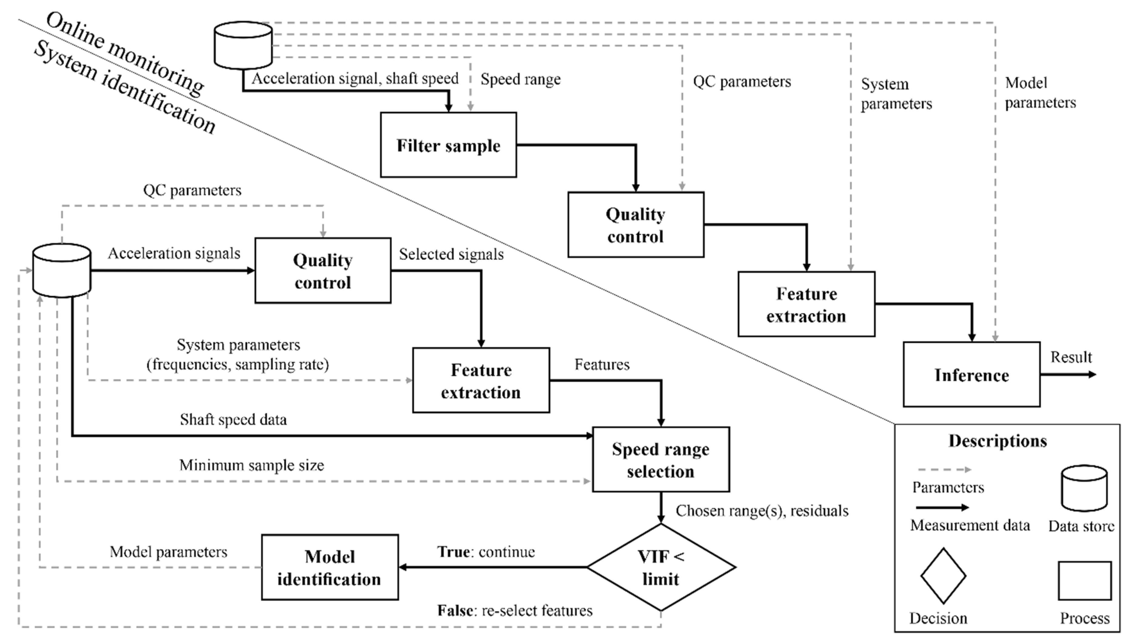
The algorithm consists of separate identification and monitoring procedures, which are illustrated in the flowcharts in Figure 2. The algorithm uses acceleration signals from selected measurement positions with the associated sampling rate and rotational speed of the shaft. The parameters used by the algorithm include user-defined and system-specific parameters and parameters identified from the training data. The parameters are summarized in Table 2 and explored more in the following sections.
Section 2.2.1, Section 2.2.2, Section 2.2.3, Section 2.2.4, Section 2.2.5, Section 2.2.6 and Section 2.2.7 clarify the different processing stages of the algorithm. Section 2.2.1 introduces the quality control of acceleration signals. The challenges of feature selection and the choices made in this study are discussed in Section 2.2.2. Section 2.2.3 focuses on the residual calculation based on the linear regression models. Section 2.2.4 introduces the method for the selection of shaft speed based on the checks of normal distribution by using the automated procedure. Section 2.2.5 introduces the multicollinearity check, which is shown in Figure 2 as the only decision block in the system identification part. The probabilistic model whose parameters are identified in the model identification process is discussed in Section 2.2.6. Finally, the probabilistic monitoring with squared Mahalanobis distance in the inference process is presented in Section 2.2.7. The inference process estimates if the system is operating in the expected condition or in a changed condition, based on the model defined in the identification stage.

2.2.1. Data Quality Control

In data quality control, the acceleration signals are discarded if their quality is inappropriate for automated condition monitoring. The signals may become adversely affected by the movements of the vessel, by the maneuvering of the thruster or by other disturbances in the measurement system. The disturbed signals are not accepted in condition monitoring and must be identified based on automated procedures. On the other hand, the rejection of useful signals should be avoided.
Therefore, a sample is rejected due to the following reasons:
  • The range of moving average of the acceleration signal is greater than a predefined limit.
  • The acceleration values are constant.
  • The absolute mean of the acceleration signal is greater than a predefined limit.
In this study, the range limit for the moving average was set 0.5 × 9.81 m/s2 (or 0.5 g) in the moving windows of 100 data points. The window size should be relatively large to avoid the rejection of signals with large impulses inflicted by defects. The limit for the absolute mean was set 2 g but a lower limit could be preferable in the practical application with a lot of data. In the signal processing stages that follow quality control, the mean must be subtracted from the accepted signals in order to obtain commensurable values in feature extraction.
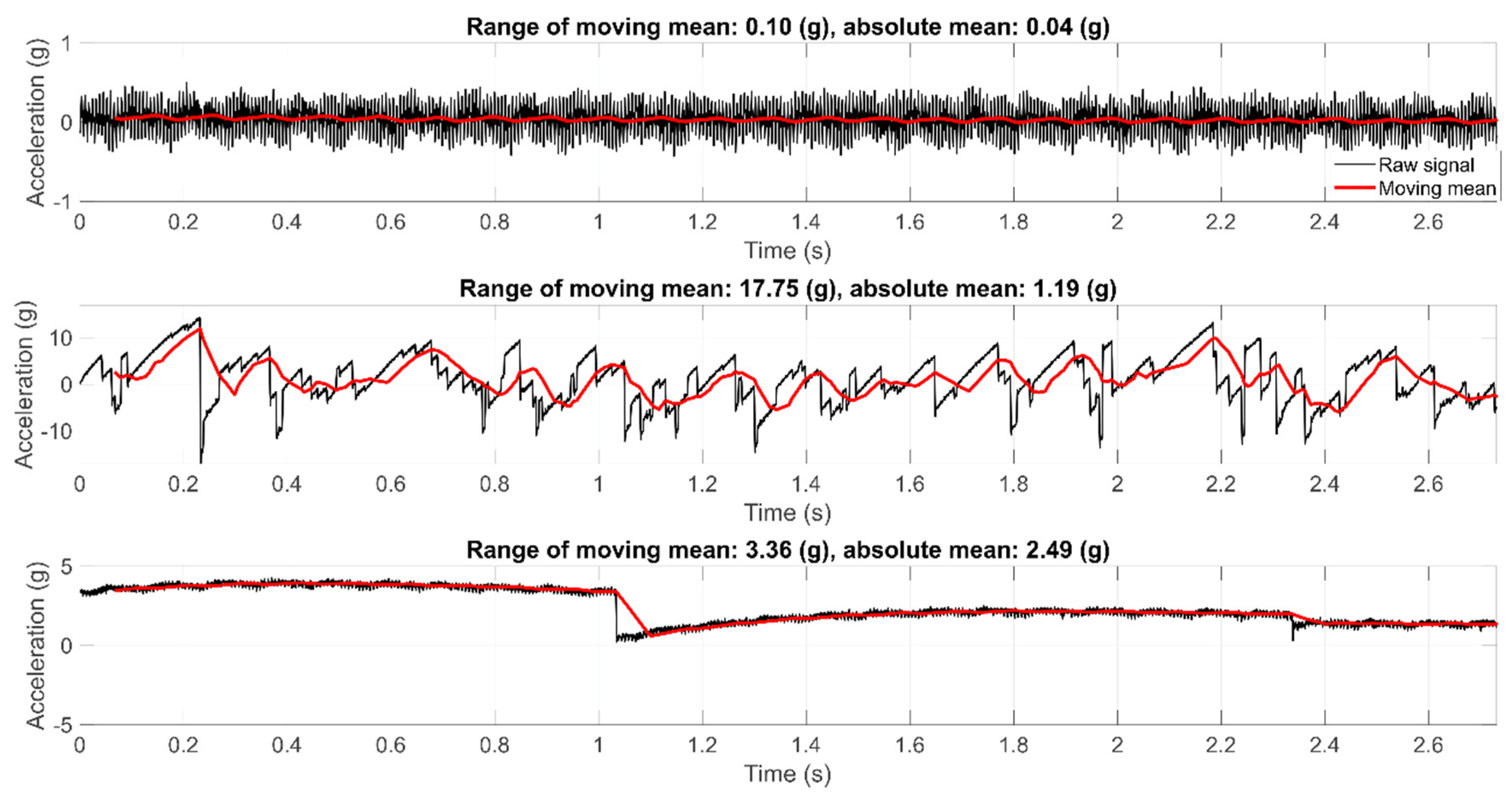
Figure 3 provides a demonstration of the quality control for three signals. The signal shown on top was accepted based on all checks, whereas the signal in the middle was rejected based on the range of moving average. The signal on the bottom was rejected based on the range of moving average and absolute mean checks.

2.2.2. Feature Extraction

The number of feature extraction methods proposed for the bearing diagnosis [21,22], gear diagnosis [23] and other condition monitoring applications [24] is immense. The methods are traditionally based on the time domain, frequency domain or time-frequency domain processing [25], and more recently the techniques of feature learning [9,26] and cyclostationary analysis [27,28] have become popular in the scientific community. The frequency domain methods are useful in the identification of the symptoms that appear as regular impulses in the signals. On the other hand, the practical applications may have irregular symptoms [29], which may be revealed only in the time domain analysis. Furthermore, the time-frequency domain methods could be useful in the acceleration and deceleration stages of the operation [30].
The features should have the capability to indicate the symptoms of defects individually or together. The symptoms can sometimes be enhanced with various signal processing techniques [21,31] and the features that reveal changes together could be selected based on some search algorithm [32] that optimizes the prediction accuracy. However, the computationally optimized signal processing parameters [33] and features [34] are prone to become case-dependent to the data sets analyzed, and then, the selections may not be useful for other data sets. In practical applications, the new data may reflect new symptoms which are not known by the models trained [10,35].
The effects of the features on the selected model must be considered as well. For example, features that correlate strongly with other selected features may bring uncertainty to parameter estimation [36,37]. Such feature correlations are sometimes reduced based on dimensionality reduction techniques, such as Principal Component Analysis [13,15], but the use of unnecessary features in the original input domain magnifies the uncertainty of inference. Moreover, many of the features are sensitive not only to damage but also to environmental and operational variations [19]. The separation of changes caused by defects from other changes requires consideration.
Therefore, the use of expert information in the selection of input data for a condition monitoring algorithm is essential. A good practice is to first select the features which famously have the diagnostic relevance, and secondly, to use additional tests which confirm their suitability to the selected modeling method (see Section 2.2.4 and Section 2.2.5). In this study, the monitoring was restricted to momentarily fixed rotational speed, i.e., the rotational speed changes but is constant during the recording of one sample. Therefore, only the time domain and frequency domain methods were considered. Based on the success in previous practical applications [24], the generalized norms, their ratios and other statistical features could provide an efficient solution to the feature extraction in time domain. Therefore, the generalized norm [38], also named as lp norm
ǁ x ( α ) ǁ p = ( 1 N i = 1 N | x i ( α ) | p ) 1 p ,
was applied in this study. The real number α is the order of derivative, x is displacement, N is the number of data points, and the real number p is the order of norm. Only the acceleration signals (α = 2) were considered in this study. In addition, the kurtosis, given by
K u r t o s i s = 1 N i = 1 N ( x i ( α ) μ σ ) 4 ,
was selected. The parameter μ is the mean and σ is the standard deviation. The kurtosis is a shape indicator for the distribution of the signal and it is sometimes used in the detection of defect-related impulses in the signal [24]. On the other hand, the generalized norm is sensitive to both the signal amplitude changes and to shock-like effects [38]. An additional characteristic of interest is the ratio between the shock-like effects and the general amplitude level, such as the ratio between a high-order norm and a low-order norm. Therefore, three features were selected for the time domain model and they are presented in Table 3 as features no. 1–3.
The frequency domain information in the acceleration signal is influenced by the operation of various components in the thruster. Therefore, it is useful to focus on the amplitude changes of specific frequencies in order to identify the responses of specific rotating components from the overall vibration. However, the selection of the frequencies for a predictive algorithm is challenging, because it is not known beforehand which components reveal the changes inflicted by defects.
The defects in rolling element bearings are often diagnosed based on the harmonics of defect frequencies and their sidebands [31]. Then again, the damage in gears is often diagnosed based on the gear rotating frequency, the meshing frequency and their harmonics, and sidebands [23]. Such frequency components could be monitored individually or together. In this study, several components were monitored together by computing a quantile value from them. The quantile selection is further reasoned in Section 2.2.3 because it influences the distribution of data samples, and therefore, the model performance.
The envelope spectrum is commonly used in the bearing diagnosis conducted by an expert [39]. However, the automated selection of an appropriate frequency band for demodulation is complicated [33,40], and therefore, the amplitude spectrum was used in this study instead. The computational bearing frequencies (see Table 1) exhibit some uncertainty due to the measurement precision, skidding and variations in the rotational speed. Therefore, each frequency component in this study was selected from the range [f(1 − ε), f(1 + ε)]. The parameter f is the computational frequency of the monitored component and ε is the error, which is set ε = 0.01. The component with the maximum amplitude was chosen to represent the component of interest from this range.
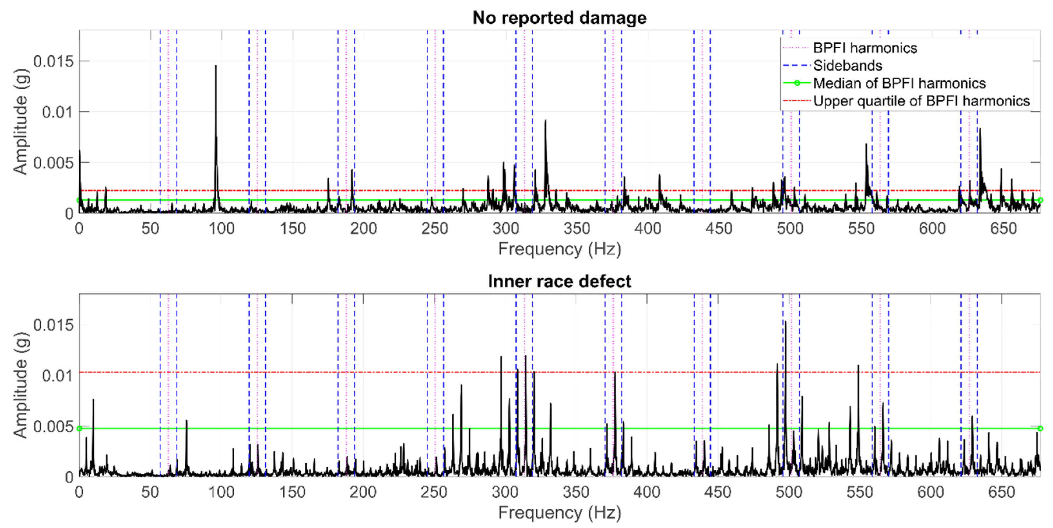
The selected features for bearing monitoring are shown in Table 3 as features no. 4–8 and the features for gear monitoring are shown as features no. 9–11. Figure 4 shows amplitude spectra from a case with no reported damage and a case with inner race defect in the bearing in thruster 1. The 1–10 BPFI harmonics and the closest sidebands are marked there separately. The median (feature no. 4) and upper quartile of the amplitudes of BPFI harmonics are marked there as well. These graphs illustrate that the feature values increased in the case of damage. The change is seen the most clearly in the fifth and higher harmonics of BPFI and sideband components in this case.
Similarly, Figure 5 shows amplitude spectra from the cases with no reported damage and wear on the gear surfaces in thruster 2. The 1–4 GMF harmonics and sidebands are marked together with the median (feature no. 9) and upper quartile computed from their amplitudes. The graphs indicate that the amplitudes of GMF harmonics and sidebands increased in the case of damage.
In automated condition monitoring, an individual frequency component may have small significance, because the fault symptoms become manifested differently when the operational state of the machine changes. Therefore, the features computed based on several frequency components could contain more diagnostic information than separate components individually. Finally, the presented features may not be optimal for the studied data sets and their optimization goes beyond the scope of this study.

2.2.3. Residual Calculation

The use of residuals of linear regression improves the applicability of the proposed method in varying shaft speeds because the strong correlation between the shaft speed and feature values is removed. This is demonstrated in Table 4 with correlation coefficients [37] calculated from the data of thruster 1. The residuals ( r i ) of linear regression can be defined by
r i = y i ( β 0 + β 1 x i ) ,
where y i is the calculated feature value, and β 0 and β 1 are the intercept and the regression coefficient of the linear regression model, identified using the least squares fitting. The predictor x i is the shaft speed and i is the sample number. The residual calculation is done in the “speed range selection” and “inference” processes in the flowcharts shown in Figure 2.
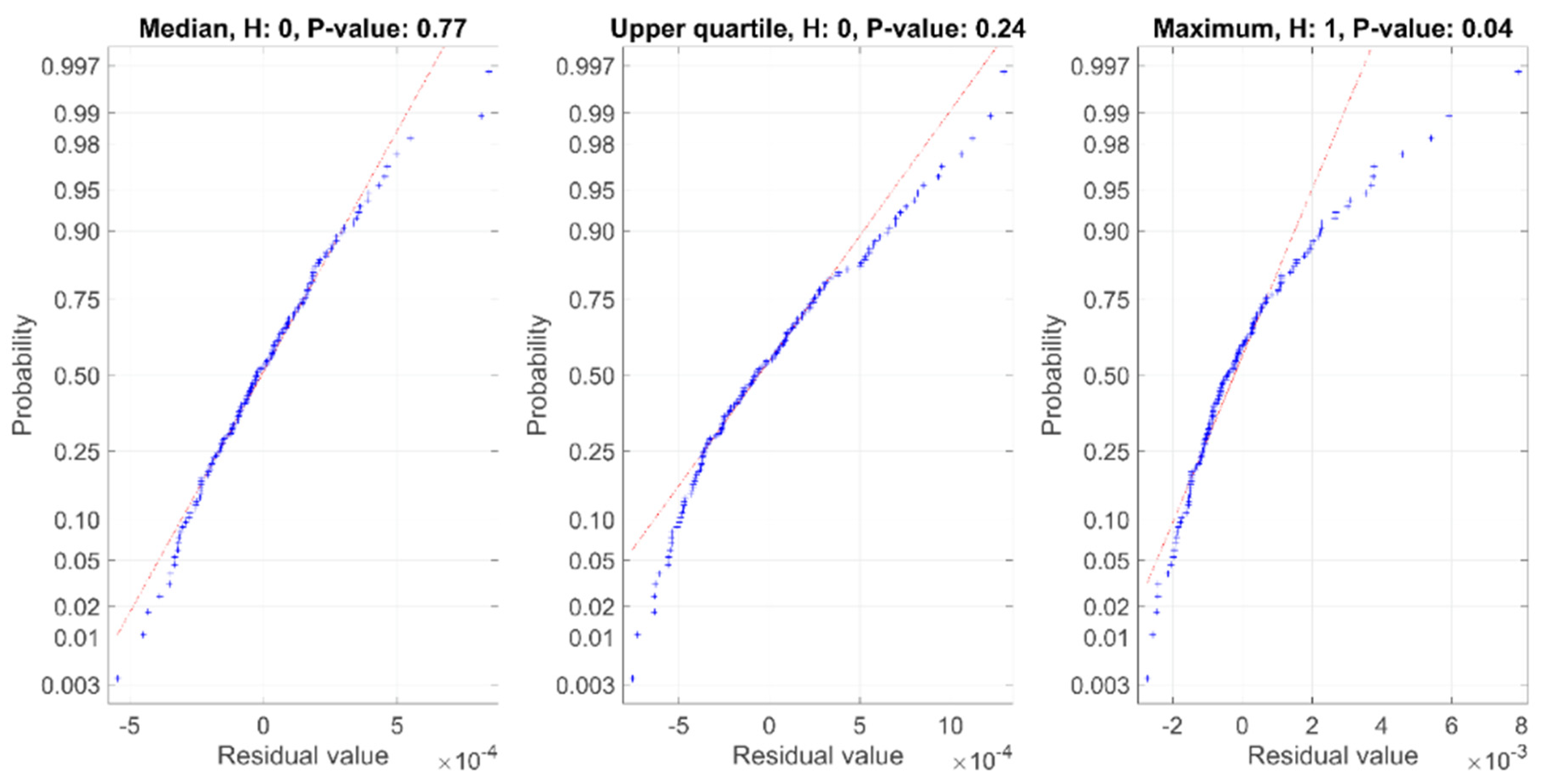
As was mentioned in Section 2.2.2, the nature of the selected feature has a significant impact on the distribution of its residual when the linear model is applied. Figure 6 demonstrates the effect of selected quantile on the distribution of data when different quantiles were calculated from 1–10 BPFI harmonics. The graphs show that the tails of the distribution moved further away from the line indicating normal distribution when high quantiles such as upper quartile or maximum were used. Additionally, the p-values of Kolmogorov-Smirnov test [41] decreased when the higher quantiles were used.
In this study, the median was selected as the quantile for the features computed from the amplitude spectrum (features no. 4–11) because the associated residual sometimes follows the normal distribution better than the residuals associated with the higher quantiles. However, this is not a general rule, and therefore, the check for normal distribution is included in the selection of the operational area, which is introduced in the following section.
The application of non-linear models for regression is beyond the scope of this study. Such models could improve the fit of the model, but there is a risk that the identified model becomes complicated and overfitted reducing its robustness in later use. The training of non-linear models would benefit from large data sets, which are often unavailable.

2.2.4. Shaft Speed Selection

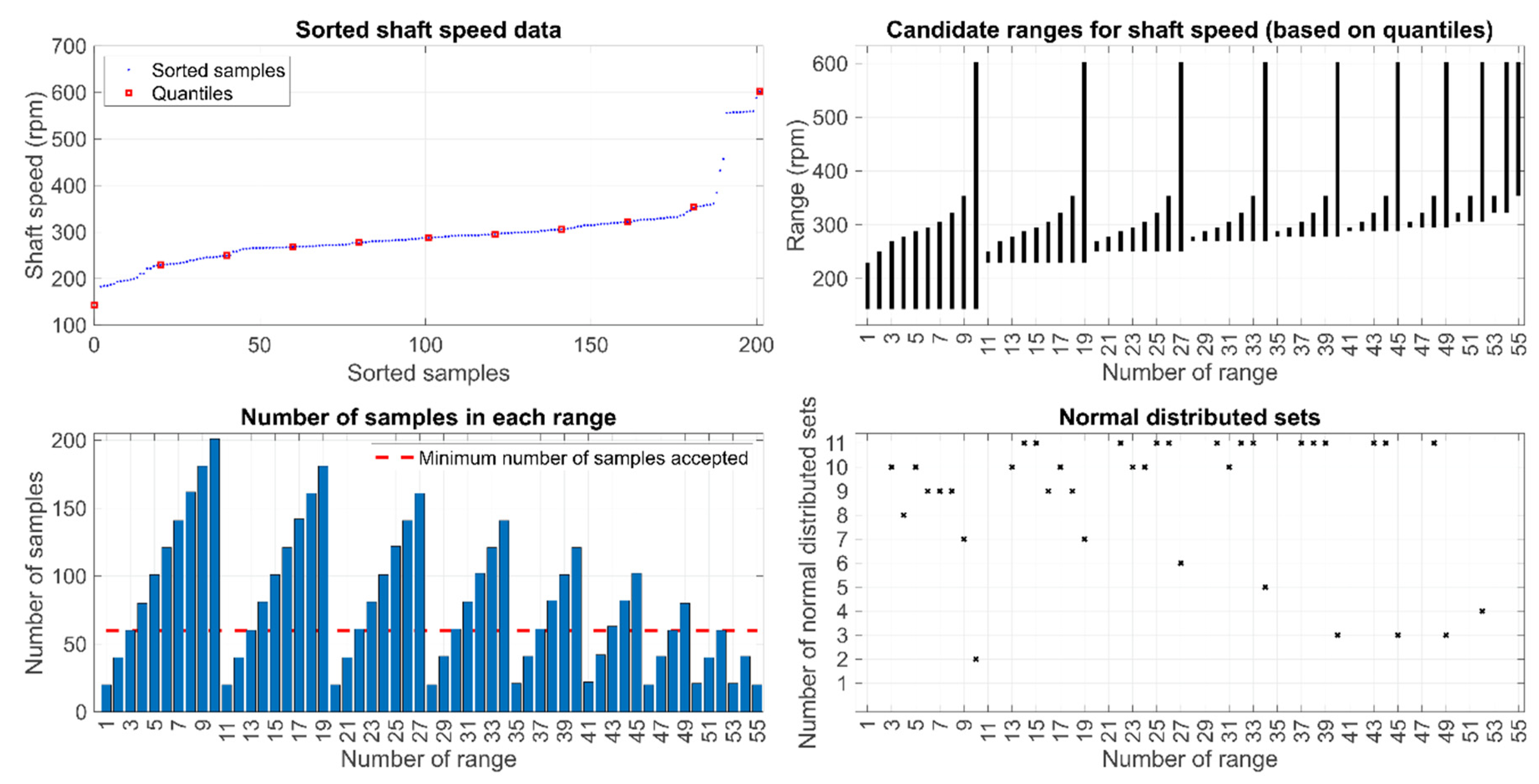
To select the appropriate shaft speed ranges for condition monitoring, statistical tests for normal distribution are included in the identification stage in the algorithm. Firstly, the samples in training data are sorted in the order of magnitude based on the shaft speed. Then, specific quantiles are computed from them which is illustrated in the upper left plot in Figure 7. In this study, the quantiles were the deciles and the zeroth quantile (minimum).
The samples are categorized in separate ranges based on the quantiles with the goal to analyze the data set in separate ranges with varying sizes. The ranges are illustrated in the upper right plot in Figure 7 where 55 separate ranges are shown. The first range covers the speed values from the minimum to the first decile, the second range covers the speed values from the minimum to the second decile, and so on.
In practice, the amount of data is limited, and therefore, the user should set a minimum sample size for each range. In the lower left plot in Figure 7, the user set the limit to 60 samples. This limit is also used later in the experiments in Section 3. If the number of samples in a range is too low, the data may not be extensive enough for the identification of a robust model.
The residual values for each feature are calculated in each range where the sample size is above the defined limit by using Equation (3). A statistical test for normal distribution is then done on each set of residual values separately assuming they are independent data sets. The one-sample Kolmogorov-Smirnov test was used in this study. It is a nonparametric test to evaluate if the empirical cumulative distribution of the data is equal to the hypothetical cumulative distribution [41]. The applied statistic is the maximum absolute difference between the empirical Cumulative Distribution Function (CDF) calculated from the data vector x and the hypothesized CDF
D * = max x ( | F ^ ( x ) G ( x ) | ) ,
where F ^ ( x ) is the empirical CDF and G ( x ) is the CDF of the hypothesized distribution, which is in this case the normal distribution. However, other suitable tests for normal distribution, such as the Anderson-Darling test [42], could be used as well. The results are presumably slightly different then.
The kstest function in Matlab® was used with the default significance level (α = 0.05 or 5%) for the null hypothesis rejection in this study. The hypothesis result H = 0 indicates that null hypothesis is not rejected at the α significance level, i.e., the data are normal distributed. The result H = 1 indicates that the null hypothesis is rejected at the defined significance level, and then the data do not come from the standard normal distribution. While the shaft speed selection is an exploratory study by nature, multiplicity corrections were neglected on the hypothesis tests [43].
In the lower right plot of Figure 7, the independent hypothesis results of the residual sets of the 11 features introduced in Table 3 are put together. The plot shows the number of normal distributed residual sets in each range. From these ranges, the algorithm selects the ranges where the highest number of normal distributed residual sets were obtained (11 in this case). If the ranges overlap, only the widest area is selected to ensure the usability of the model in as wide operational area as possible. Therefore, the range no. 26 (249.86–353.47 rpm) became selected alone in this example.
In online monitoring, the algorithm filters the samples based on the selected shaft speed ranges as indicated in the flowchart in Figure 2. If a new sample is inside the selected speed ranges, it is accepted and proceeds to the quality control process introduced in Section 2.2.1.

2.2.5. Multicollinearity Check

The squared Mahalanobis distance calculation uses the covariance information among the input variables. The inverse matrix of the covariance coefficients may become inaccurate if the variables are highly correlated [18]. The residual calculation removes the strong correlation between the shaft speed and input variables (see Table 4), but the residuals may be strongly correlated with each other. This may happen when several redundant features, such as lp norms with different order p, are used together. To elude the use of highly correlated variables, the multicollinearity of the residual sets is evaluated by using the Variance Inflation Factor (VIF)
V I F = 1 1 R j 2 ,
where R j 2 is the coefficient of determination from the regression of explanatory variable (rj) onto all other explanatory variables. If the coefficient of determination is close to one, collinearity is present and VIF is large. VIF = 1 indicates the complete absence of collinearity. As a rule of thumb, a VIF value that exceeds 5 or 10 could indicate a problematic amount of collinearity [37]. If VIF goes above the threshold, the selection of different features is recommended as shown in the flowchart in Figure 2.

2.2.6. Multivariate Normal Distribution

The model identification is done based on training data consisting of machine operation from periods where an undamaged (or healthy) condition is probable. It is assumed that the residuals follow the identified normal distributions when the system is in undamaged condition. Therefore, the residuals are modeled as multivariate normal vectors x that belong to a multivariate normal distribution with mean vector μ and covariance matrix Σ. The probability density function (PDF) of the multivariate normal distribution function is
f ( x , μ , Σ ) = 1 | Σ | ( 2 π ) d e x p ( 1 2 ( x μ ) Σ 1 ( x μ ) T ) ,
where d is the dimension of the multivariate normal distribution. In this study, the covariance matrix for each distribution was defined based on normalized residuals (μ = 0, σ = 1).
For each multivariate normal distribution, the identification of several parameters is required. The parameters are summarized in Table 5 and correspond to the “model parameters” identified from data, as shown in Figure 2. Different parameter values are identified for different shaft speed areas.
In this study, separate models were used for time domain features (no. 1–3), bearing features (no. 5–8) and gear features (no. 9–11), because the algorithm should have diagnostic ability. Therefore, three covariance matrices were identified for each shaft speed range. In total, 47 parameters were identified and saved for each selected shaft speed range with these settings. The means of residuals (μ) are approximately zero and can be replaced with zeros.

2.2.7. Probabilistic Monitoring

The deviations of calculated samples from the identified distributions are monitored by calculating the squared Mahalanobis distance in the inference process depicted in Figure 2. The squared Mahalanobis distance from a monitored sample r m to a distribution with the mean (μ) and the covariance matrix (Σ) can be defined by
D = ( r m μ ) T Σ 1 ( r m μ ) .
The monitored sample r m consists of the d regression residual values, which are normalized based on the means and standard deviations identified in the training set.
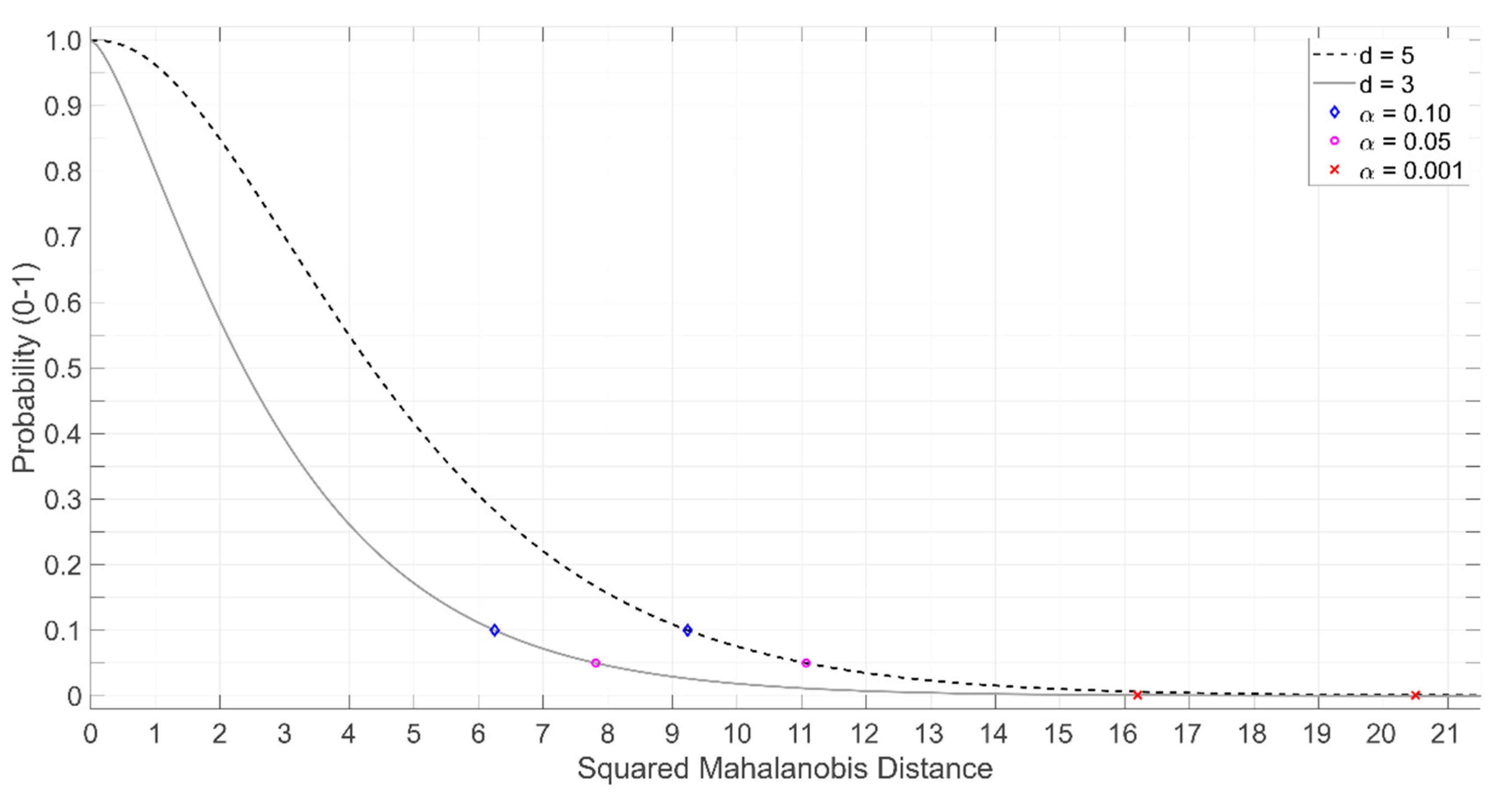
The squared Mahalanobis distance follows the chi-square distribution with d degrees of freedom, and therefore, each value can be converted into a probability [44,45]. An appropriate threshold value can be selected from the distribution to detect outliers [46] or to monitor the system health [18]. Figure 8 demonstrates the probabilities associated with D values using d = 3 and 5. In this study, the chi2cdf function in Matlab® was used for calculating the probability associated with the squared Mahalanobis distance.
The probabilistic values defined by α could be used as the reference limits to indicate if the new samples belong to the identified distribution. Jin et al. [18], for example, recommend the use of 99.9th percentile (α = 0.001) as the limit but inferred that the limit depends on the risk of system malfunction. Yu [15] used a certain number of consecutive values (=3) exceeding a probabilistic control limit as the sign of health state change in the monitored machine. In addition, the D values can be monitored in moving windows. The moving median with window size n = 5 was used in this study as an addition to the monitoring of individual values.

2.3. Classification Tests

To study the diagnostic performance quantitatively, classification tests were done in a binary setup where the methods predict the labels of samples as positive or negative, i.e., as “damage” or “no damage,” respectively. The actual labels were defined based on the reports made by ISO certified vibration analysts of the manufacturer.
Two different approaches introduced in Section 2.3.1 were used to evaluate the performance of the proposed method. The method was compared with the reference classifiers, introduced in Section 2.3.2. The performance of the methods was evaluated by using four criteria as presented in Section 2.3.3. To achieve an estimate for the unbiased generalization performance, the methods were compared by using the nested cross-validation approach discussed in Section 2.3.4.

2.3.1. Classification Approaches for the Proposed Method

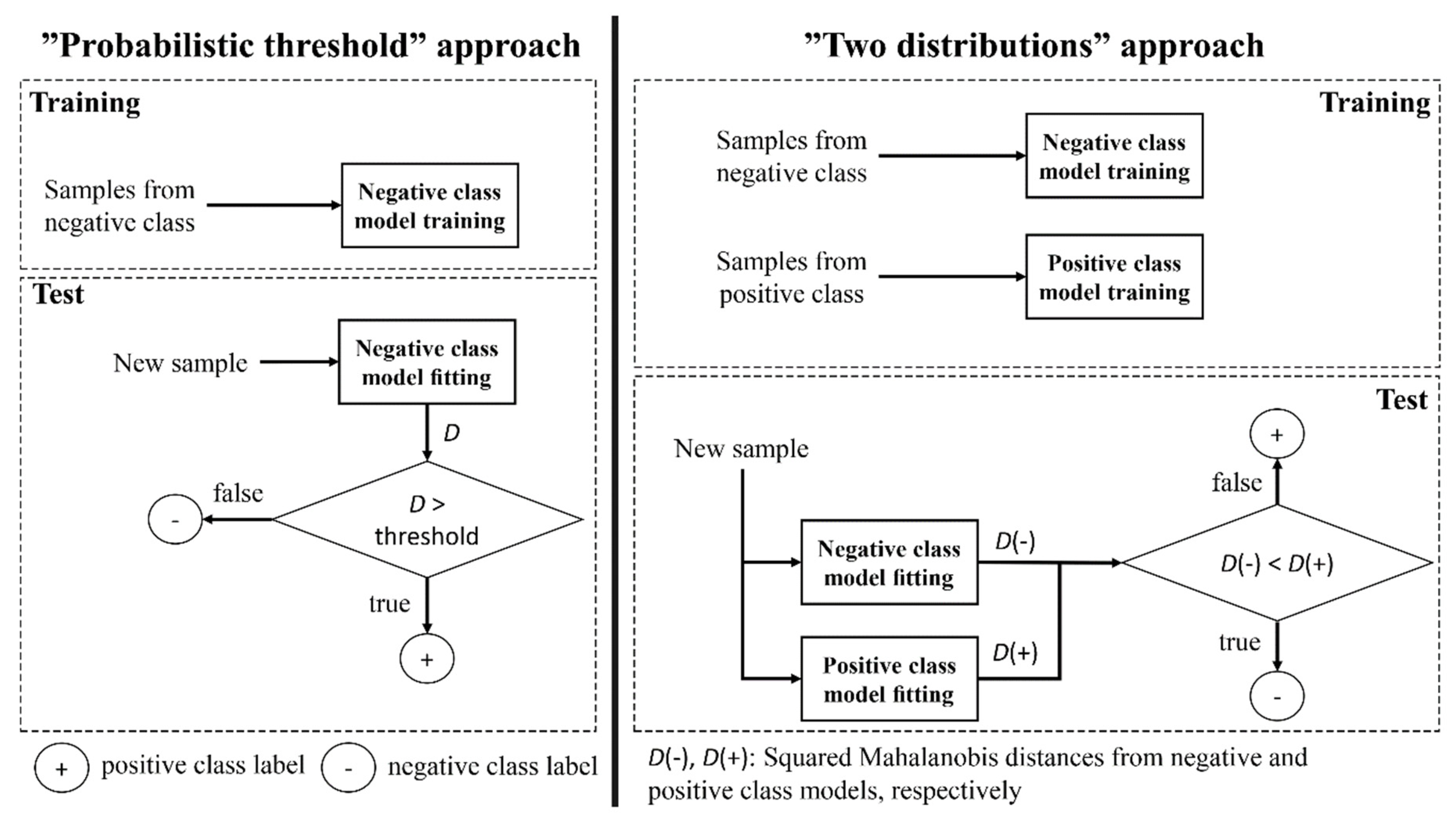
The first approach utilizes probabilistic thresholds α to classify individual samples in classes. If a sample defined by squared Mahalanobis distance (D) is below the threshold defined by α, the sample comes from the defined distribution and is a member of the negative class. Otherwise, it is a member of the positive class. Three different thresholds α = {0.1, 0.05, 0.001} were tested to separate the classes from each other. The models were trained by using only the data from the negative class. This approach is named as “probabilistic threshold” here.
To obtain a more equal approach to the actual classifiers from the training perspective, an alternative approach called “two distributions” was used as well. Two different models were trained by using the samples of the positive and negative classes in separate models. New samples were then classified by estimating D values using both models and by labeling the sample based on the lower value. For example, if the model trained based on the positive class produced a lower value than the model trained based on the negative class, the sample belonged to the positive class.
Figure 9 illustrates the flowcharts for both approaches. The quality control of signals was done in advance with parameter values shown in Table 2. The shaft speed range of the samples was defined before classification tests based on the identification data, introduced in Section 2.1.3, by using the approach presented in Section 2.2.4. The training of the model included the identification of the parameters presented in Table 5.

2.3.2. Reference Methods

Fault classification based on machine learning algorithms has been widely studied during the last decades. Some of the commonly applied classifiers were chosen as the reference methods here. They include k-Nearest Neighbor (k-NN), Linear Discriminant Analysis (LDA), Support Vector Machines (SVM) and AdaBoost M1. Each of these algorithms have been previously applied in machine diagnosis studies, such as in [47,48,49,50], respectively. The details of theoretical bases and implementations of the classifiers are reported in the previous literature and are, therefore, omitted here.
The hyperparameter values of the classifiers were optimized based on the mean accuracy in the inner resampling loop of the nested cross-validation by using the exhaustive search. The tested values are shown in Table 6. The features shown in Table 3 were used as the input variables for the classifiers after normalizing them to unit variance and zero mean. The computations were done by using Matlab® 2019a.

2.3.3. Evaluation Criteria

The classifier performance was evaluated based on the accuracy, precision, recall and specificity. Accuracy can be defined as
A c c u r a c y =   T P + T N T P + F P + T N + F N ,
where TP is the True Positive count, TN is the True Negative count, FP is the False Positive count and FN is the False Negative count. Accuracy was used in this study as the criterion to be maximized in the hyperparameter optimization in the classifiers.
Precision reveals the accuracy of the positive predictions. Low precision indicates that the classifier labels samples falsely as positive which may result in an increased amount of useless maintenance actions. Precision is defined by
P r e c i s i o n =   T P T P + F P .
Recall (or sensitivity) shows the ratio of predicted true positives to the total number of true positives. Low recall indicates that the classifier labels the samples of the positive class falsely as negative class which increases the risk that the damaged machine will be kept in operation although it should be taken to service. Recall is defined by
R e c a l l =   T P T P + F N .
Specificity shows the ratio of predicted true negatives to the total number of true negatives. Low specificity indicates that the samples of the negative class are falsely labeled as positive class which is a harmful feature as it increases the number of false alarms. Specificity is defined by
S p e c i f i c i t y =   T N T N + F P .

2.3.4. Nested Cross-Validation

The nested cross-validation was applied to estimate the unbiased generalization performance of the classifiers. The outer resampling loop, which was used for the performance evaluation, applies the repeated random sub-sampling validation [51]. The inner resampling loop, which was used for hyperparameter optimization in classifiers, applies the 10-fold cross-validation which is programmed in the Matlab® functions presented in Table 6.
As shown in Section 2.2.6, the proposed algorithm has the requirement of normal distributed data for model identification, and therefore, a specific approach for the random sampling in the outer resampling loop was developed. The approach is illustrated in Figure 10 with a flowchart.
As discussed in Section 2.3.1, the appropriate shaft speed range was first identified based on the full set of samples in the identification data. Although the data set in this range is normal distributed, the subsets of data points in this set may not be normal distributed when they are sampled randomly for the training sets. Therefore, the check for normal distribution was done again for each randomly sampled training set, as shown in Figure 10, and only the sets that had normal distributed residuals were accepted for training sets. The check was done separately for both the data in negative and positive classes, because both classes were used to train the models in “two distributions” approach.
Based on the inferences in [52], 50% of the data was used for both the training and test sets, i.e., the split ratio was 1:1. The number of random iterations in the outer resampling was 3 × N, where N is the sample size. In both the training and test sets, the balanced division between the negative and positive classes was used. Each classifier, including the reference methods, was trained and tested by using the same samples.

3. Results and Discussion

Section 3.1 demonstrates the performance of the algorithm based on the actual measurement data that contains both the undamaged and damaged condition in the thrusters. The performance in classification is then compared with the reference methods in Section 3.2. The results and additional research recommendations are further discussed in Section 3.3.

3.1. Application on Data Sets

3.1.1. Thruster 1

The data set for model identification with 207 samples included shaft speed in the range 143.32–602.53 rpm. The number of accepted samples in quality control was 201 and the selected shaft speed range was 249.86–353.47 rpm, which consisted of 141 samples (see Figure 7). The derived parameter values and covariance matrices of the identified models are presented in Appendix A.
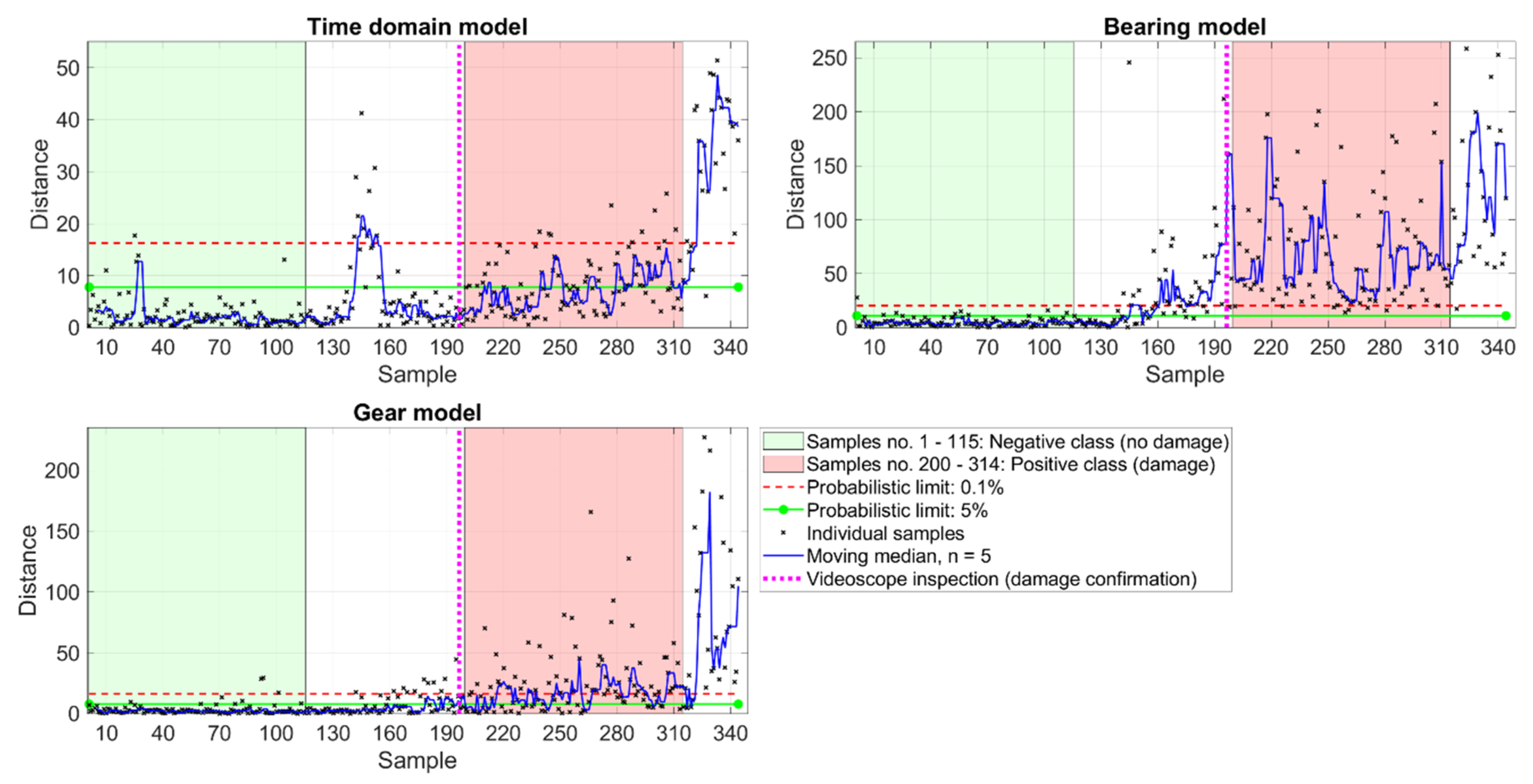
The application of the models is demonstrated in Figure 11 where the first 141 samples were used to train the models. The samples 142–344 are new independent samples inside the selected shaft speed range and they correspond to a 364-day period, indicating there were various days in which accepted samples were missing in the selected shaft speed range.
Two periods with the same length are indicated in the plots to represent negative class and positive class. The data used for these samples were used for classification in Section 3.2 as well. The defects were confirmed based on the videoscope inspection after sample no. 196.
Figure 11 indicates that the squared Mahalanobis distance values had an increasing trend after the training period indicating that the operation began to diverge from the operation in the training period. Perhaps the moving median gives a clearer indication of this progress. The bearing model especially gave distinct indications of change around samples no. 142–195, which corresponds to a 102-day period before the videoscope inspection. In addition, the time domain model showed some changes after the 141 first samples and the gear model showed deviations more regularly at the end of the complete period shown. In conclusion, the models together suggest that the condition changed in the thruster based on the observations in the monitored speed range.

3.1.2. Thruster 2

The data set with 162 samples for model identification included shaft speed in the range 296.14–748.40 rpm. All the samples were accepted in quality control and the selected shaft speed was 296.14–459.94 rpm, which consisted of 113 samples. The identified parameter values of this operational area are shown in Appendix A.
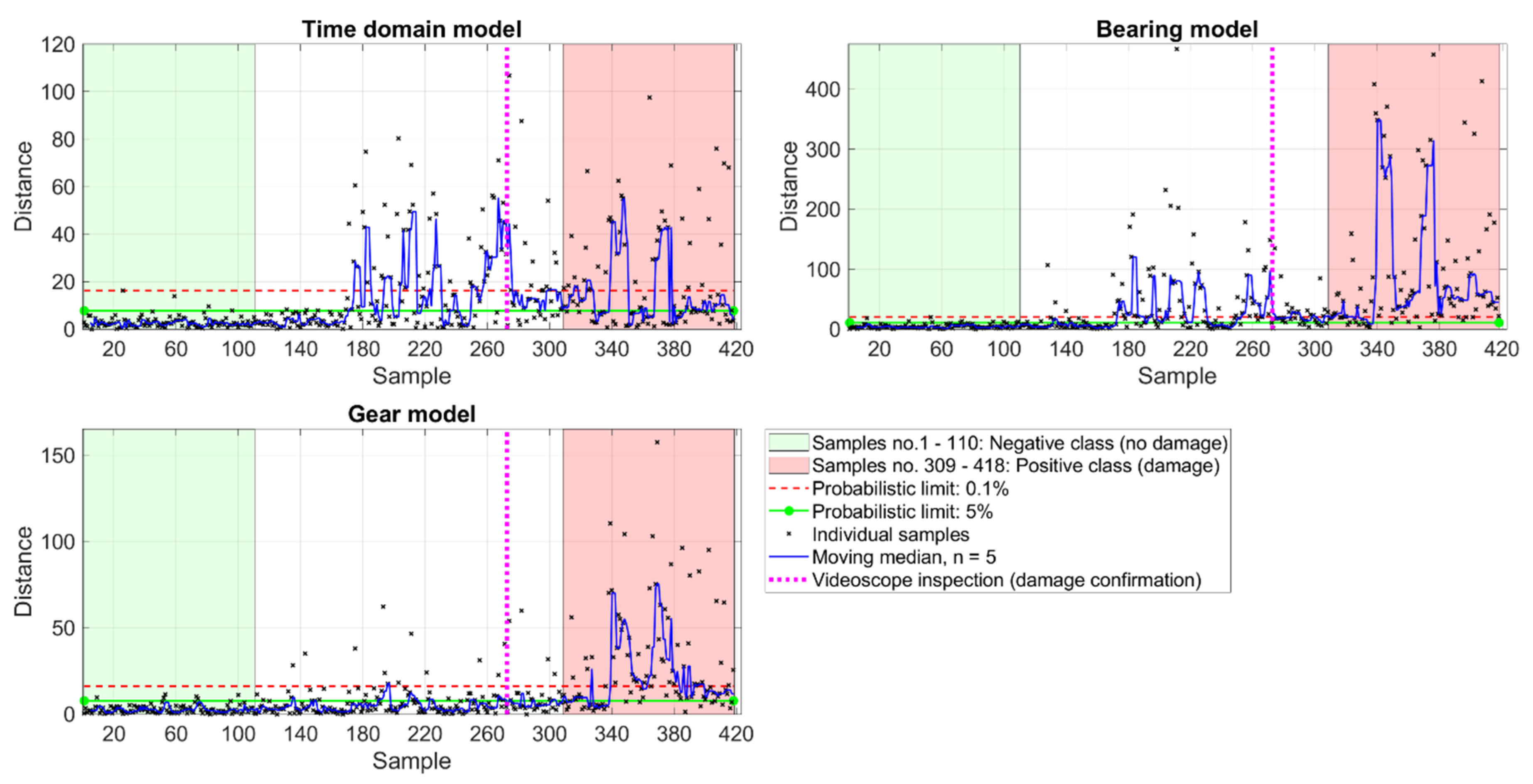
The application of the models in monitoring is demonstrated in Figure 12 where the first 113 samples were used to train the model. Samples 114–418 are new independent samples in the selected shaft speed range and they correspond to a 370-day period. The defects were confirmed based on videoscope inspection after sample no. 272. The periods marked with negative and positive classes were used for the classification in Section 3.2.
The monitoring results for thruster 2 shown in Figure 12 have similarity to the behavior in Figure 11. The monitored D values started to increase after the training period. Especially, the time domain and bearing models showed high values regularly on the 81-day period shown by samples no. 170–272 before the videoscope inspection. The gear model gave clearer indications of change during the period marked as positive class.

3.2. Classification Tests

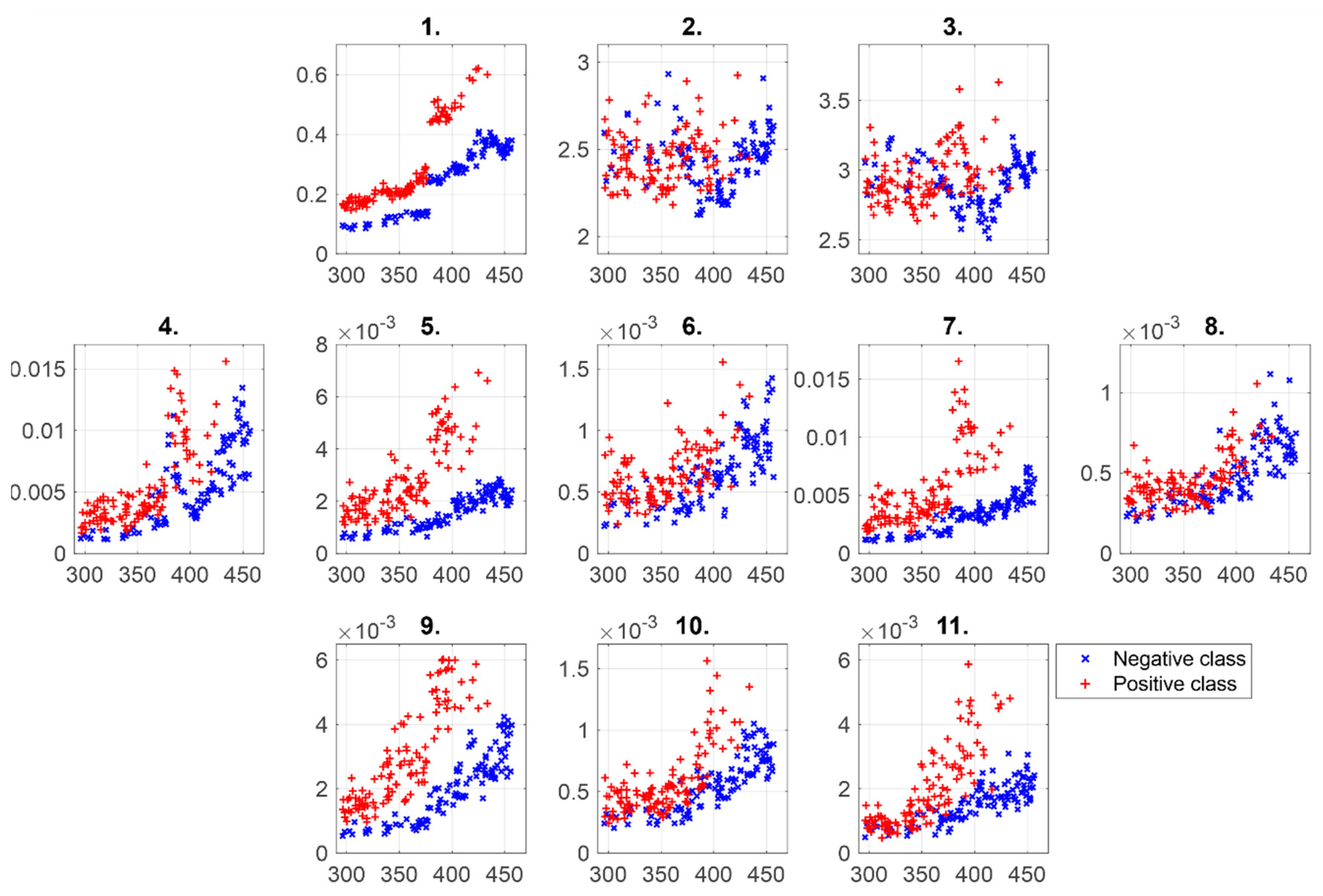
The data used for classification are shown as scatter plots between the shaft speed and feature values in Figure 13 and Figure 14 for thrusters 1 and 2, respectively. Some of the features, such as features no. 1, 4, 7 and 9, show distinct clusters between the classes in both data sets. However, the patterns are different although the same type of damage was reported on both thrusters. For example, feature no. 5 does not show clear difference between the classes in 300–350 rpm in Figure 13, whereas Figure 14 shows some difference between the classes. Some of the features, such as features no. 2 and 3, do not show distinct differences between the classes in neither of the figures. Many features had a positive correlation with the shaft speed, but it is not fully linear, as shown by features no. 1 and 9 in Figure 14. In addition, the feature values had a discontinuity around 380 rpm shaft speed indicating there could be two separate operational areas.
Figure 15 shows the classification results for the data set of thruster 1. The bearing feature set had the highest accuracy from different feature sets in general. At least 90% accuracy was reached with the bearing feature set by each method apart from the AdaBoost M1, which had low accuracy (50.18%). The highest test accuracy (95.51%) was achieved by using “probabilistic threshold” approach with α = 0.001. The other criteria (precision, recall, specificity) reached over 94% value then as well.
The time domain feature set resulted in the highest test accuracy, 88.78%, with “two distributions” approach. The test accuracies of the reference methods were in the range 79.46–82.92% but AdaBoost M1 suffered from overfitting because the training accuracy was 99.51%. The “probabilistic threshold” approach had the lowest test accuracy 56.13% (α = 0.001) to 75.68% (α = 0.1).
With the gear feature set, “probabilistic threshold” approach reached test accuracies 75.01–81.79% whereas “two distributions” approach had the test accuracy 84.47%. These accuracies are lower than the test accuracies of some of the reference methods, the range of which was 83.98% (AdaBoost M1) to 89.28% (k-NN). AdaBoost M1 suffered from overfitting while the training accuracy was 97.44%.
The highest test precision (98.58%) was achieved by using LDA with the bearing features as input variables. The highest recall (100%) was achieved by using “probabilistic threshold” approach (α = 0.1) with the bearing feature set. By using α = 0.05 or “two distributions” approach, the value was almost as high. The highest specificity (99.96%) was achieved by using AdaBoost M1 with the bearing features as input variables, but the accuracy was poor indicting that the classification was unsuccessful. With the precision, recall and specificity criteria, one must acknowledge that the hyperparameters in the classifiers were optimized by maximizing the test accuracy in the inner resampling loop. Different results may be obtained by using a different criterion.
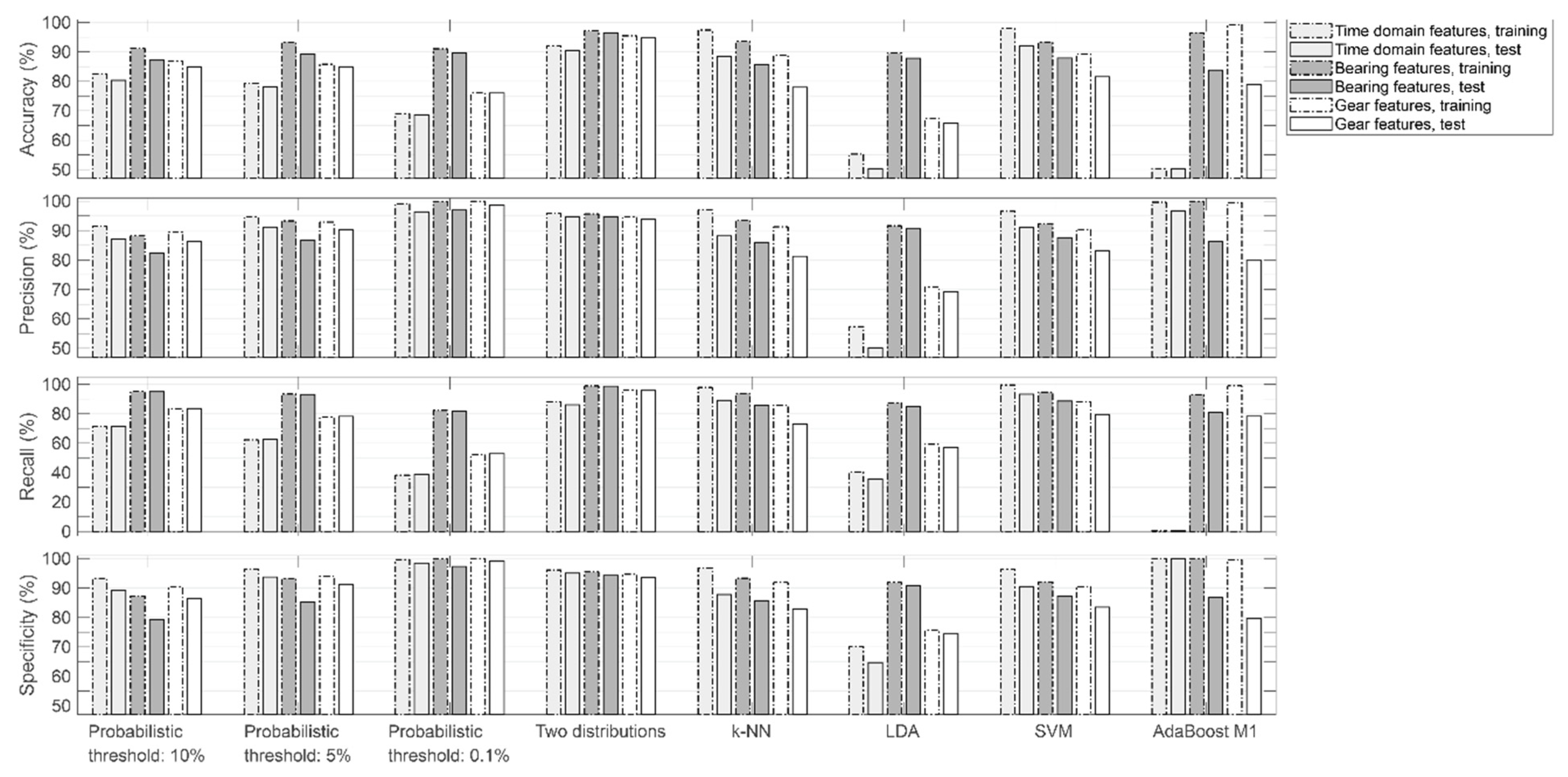
In the data set of thruster 2, the predictive power of the different feature sets was more equal than in the other data set. This can be inferred especially from the results of “two distributions” approach, the performance of which was relatively similar with different feature sets, as shown in Figure 16. Other approaches like SVM and k-NN supposedly give (fainter) indications of the more equal predictive power as well when all the performance criteria are examined together.
With bearing features, the highest test accuracy, 96.51%, was obtained by using the “two distributions” approach, while the second highest accuracy, 89.62%, was achieved by using the “probabilistic threshold” approach with α = 0.001. The reference methods had accuracies in the range 83.84% (AdaBoost M1) to 87.88% (SVM).
With time domain features, the highest test accuracy, 91.91%, was achieved by using SVM. Then again, two other reference methods, LDA and AdaBoost M1, had test accuracies below 50.40%. The test accuracy of “two distributions” approach was 90.55%, while the “probabilistic threshold” approach had accuracies in the range 68.69% (α = 0.001) to 80.30% (α = 0.1).
With gear features, the highest test accuracy, 94.68%, was achieved by using the “two distributions” approach. The “probabilistic threshold” approach had test accuracies in the range 75.97–84.99% and the reference methods had accuracies in the range 65.79% (LDA) to 81.54% (SVM).
The highest precision (98.58%) was achieved by using the “probabilistic threshold” approach with α = 0.001 when the gear features were used as input variables. The highest recall (98.76%) was achieved by using the “two distributions” approach with the bearing features as input variables. The highest specificity (99.98%) was achieved with AdaBoost M1 with the time domain features as input variables, but the accuracy was only 50.35%, indicating that the classification was unsuccessful.
Based on Figure 15 and Figure 16, the precision and specificity increased together with decreasing α in “probabilistic threshold” approach, apart from the precision with the time domain features in Figure 15. This suggests that the number of false positive predictions go down when the limit value for D is set higher (i.e., α is set lower). On the other hand, this increases the risk that the number of false negatives grows and then recall decreases, which is shown in Figure 15 and Figure 16.

3.3. Discussion

3.3.1. Significance of Results

Classification results show that the threshold (α) had a significant effect on the classification accuracy when individual samples were classified. This is seen, for example, with the time domain feature set of thruster 1 while the accuracy varied between 56% (α = 0.001) and 76% (α = 0.1). The selection of the threshold is a trade-off between the number of false positives and false negatives. In general, the higher threshold limit (e.g., α = 0.001) results in the lower the number of false positives, but also the number of false negatives grows. With the low threshold limit (α = 0.1), the number of false positives increases and the number of false negatives decreases.
In the light of this challenge, it could be useful to monitor the squared Mahalanobis distance in moving windows, as shown in Figure 11 or Figure 12, thus reducing the variation of the values used for inference. The use of moving mean or median is a standard approach in statistical process control [53]. Alternatively, a long enough segment of consecutive points on the other side of the threshold could indicate the change in condition, as was inferred in [15].
The accuracy of the “two distributions” approach indicates that training separate models for normal and damaged conditions could be useful. However, the fault patterns in the signals should then be relatively fixed in the operational areas monitored, which is not certain, as indicated by the different patterns in Figure 13 and Figure 14. In addition, the separation of the symptoms of superposed faults and other disturbances in signals is also required, unless it is probable that they occur together. Moreover, the correct labeling of each data sample in large data sets used for model training is often unrealizable without a robust automated approach to it.
Therefore, the classification results are approximate and not a definitive proof of the performance of the methods. A predicted false negative, for example, could be a result of the fact that the sample does not contain characteristics of the defect even though the true label was set positive. This highlights the importance of a well-planned and executed sample selection to obtain significant results [54].

3.3.2. Suggestions for Future Research

The operational state of the thruster was unknown apart from the rotational speed of the pinion shaft. In practice, the steering angle changes and the vessel may be in transit or performing a task using the dynamic positioning. These factors presumably have effects on the acceleration signals, and therefore, their correlations with the signals should be further analyzed in various operational circumstances. The utilization of such information could reduce the variation in inference, if the information was used to filter samples or to predict feature values, for example.
The data used for system identification are based on the normal operation of the azimuth thrusters and can only be relied on during such operations. Therefore, the identified system cannot fully describe the behavior of the physical one when it encounters high domain oscillations and vibrations inflicted by extreme conditions. The identification of the entire operational domain is limited by the associated costs and the lack of facilities to gather the ideal data sets for that. Therefore, alternative approaches should be developed to improve the system identification procedure.
In addition, the uncertainty of inference should be studied by focusing on the effects of feature values and the parameters shown in Table 2. Furthermore, the sample size requirements [55] for the model training should be studied to enhance the robustness of the models while the amount of training data is limited in practice. Additionally, the testing of different hypothesis tests for normal distribution could provide alternative views to the operational area selection.
As shown by the overlapping classes in Figure 13 and Figure 14, the feature sets used in this study were not optimal for the fault cases studied. Undoubtedly, clearer difference between classes could be obtained by using wrapper methods [32] on large feature sets during classifier training or by using other criteria [34]. However, these approaches give feature sets that are specific to the data sets analyzed, and their benefits for new data sets remain unclear. In addition, the various methods for signal processing could increase the sensitivity to defects, which can be inferred from the success in previous industrial applications [24].
Finally, a change detected in the operation is not necessarily inflicted by a defect in the monitored system. Therefore, reliable references should be identified for the implemented model to verify its performance. In the development stage, this could be done based on human expertise, but in the long run, automated adaptation mechanisms [56] may be required, where the use of synchronized data from redundant sensors could be useful.

4. Conclusions

A probabilistic condition monitoring algorithm was introduced and validated based on noisy, real-world acceleration signals from two azimuth thrusters used in an operating drill ship. The algorithm contributes to the general problem of sample selection by including automated procedures for the control of data quality and for the selection of shaft speed areas to be monitored. The automation accelerates the implementation of the method in a large fleet of thrusters.
The method was tested against reference classifiers and the results were obtained through an unbiased cross-validation approach. The results suggest that the algorithm performed slightly better in a binary classification task relative to the reference classifiers when the bearing features were used in the “probabilistic threshold” approach. With the least sensitive feature set (i.e., time domain features), the best reference classifiers were more accurate. The use of the “two distributions” approach with two models generally improved the performance over the “probabilistic threshold” approach, which applied one model.
The classification results suggest that the monitoring of individual samples of squared Mahalanobis distance against some threshold value results in various false positives and negatives. This was also confirmed in the monitoring tests. Therefore, the smoothed trend given by the moving median could be a more useful indicator for the practical application.
The reduction of variation in monitoring should be further pursued. The use of additional information on the thruster operation, such as the momentary steering angle, together with the information on vessel movement could improve the accuracy. Moreover, the contributions of model parameters to the uncertainty in inference require further analysis leading the way towards the online maintenance of the model.

Author Contributions

Conceptualization, R.-P.N. and M.R.; methodology, R.-P.N.; software, R.-P.N.; validation, R.-P.N.; formal analysis, R.-P.N.; investigation, R.-P.N.; resources, L.S.; data curation, R.-P.N.; writing—original draft preparation, R.-P.N.; writing—review and editing, R.-P.N., M.R., J.K.-R., L.S. and F.F.; visualization, R.-P.N.; project administration, J.K.-R.; funding acquisition, J.K.-R. and R.-P.N. All authors have read and agreed to the published version of the manuscript.

Funding

This research was funded by Business Finland during the Reboot IoT Factory program.

Institutional Review Board Statement

Not applicable.

Informed Consent Statement

Not applicable.

Data Availability Statement

Data sharing is not applicable to this article due to legal issues.

Acknowledgments

We would like to thank the CMS team of Kongsberg Maritime Finland Oy for the data, support and expertise, and Remion Oy for their collaboration during the project.

Conflicts of Interest

The authors declare no conflict of interest. The funders had no role in the design of the study; in the collection, analyses, or interpretation of data; in the writing of the manuscript, or in the decision to publish the results.

Appendix A

The identified parameter values for thruster 1 in the speed range 249.86–353.47 rpm are shown in Table A1. The means (μ) of residual values are omitted (μ ≈ 0). The VIF values were computed by using only the residuals that are together in the models: Time domain model had features no. 1–3, the bearing model had features no. 4–8 and the gear model had features no. 9–11. The low values indicate that the models did not suffer from high multicollinearity.
Table A1. Identified parameter values of thruster 1 data set.
Feature No.σβ0β1VIF
19.09 × 10⁻³−30.42 × 10−3415.16 × 10−61.15
2194.62 × 10−32.53228.01 × 10−61.81
3171.79 × 10−33.38−1.04 × 10−31.62
4236.88 × 10−6−2.00 × 10−39.95 × 10−61.15
5231.94 × 10−6−256.99 × 10−63.44 × 10−61.09
688.18 × 10⁻⁶−725.54 × 10−63.55 × 10−61.04
7153.40 × 10−6−2.04 × 10−39.99 × 10−61.11
855.34 × 10⁻⁶−811.19 × 10−63.61 × 10−61.03
994.55 × 10⁻⁶−714.60 × 10−64.29 × 10−61.55
1071.53 × 10−6−498.69 × 10−62.44 × 10−61.02
11140.14 × 10−6−240.91 × 10−62.43 × 10−61.55
The identified covariance matrices for the time domain model (Σ1), bearing model (Σ2) and gear model (Σ3) of Thruster 1 were as follows:
Σ 1 = ( 1 359.40 × 10 3 173.87 × 10 3 359.40 × 10 3 1 617.53 × 10 3 173.87 × 10 3 617.53 × 10 3 1 )   ,
Σ 2 = ( 1 213.16 × 10 3 115.86 × 10 3 244.48 × 10 3 20.74 × 10 3 213.16 × 10 3 1 121.86 × 10 3 70.23 × 10 3 16.63 × 10 3 115.86 × 10 3 121.86 × 10 3 1 85.52 × 10 3 26.46 × 10 3 244.48 × 10 3 70.23 × 10 3 85.52 × 10 3 1 164.39 × 10 3 20.74 × 10 3 16.63 × 10 3 26.46 × 10 3 164.39 × 10 3 1 ) ,
Σ 3 = ( 1 108.25 × 10 3 592.75 × 10 3 108.25 × 10 3 1 110.76 × 10 3 592.75 × 10 3 110.76 × 10 3 1 )   .
The identified parameter values for thruster 2 in the speed range 296.14–459.94 rpm are shown in Table A2. The low VIF values indicate that the models did not suffer from high multicollinearity.
Table A2. Identified parameter values of thruster 2 data set.
Feature No.σβ0β1VIF
135.39 × 10⁻³−637.20 × 10−32.26 × 10−31.09
2164.37 × 10−32.32315.05 × 10−62.71
3164.33 × 10−32.85141.03 × 10−62.59
42.07 × 10⁻³−18.38 × 10−359.99 × 10−61.57
5282.56 × 10−6−3.64 × 10−313.26 × 10−61.10
6180.64 × 10−6−1.38 × 10−35.13 × 10−61.18
7727.55 × 10−6−9.51 × 10−332.60 × 10−61.52
8120.02 × 10−6−893.59 × 10−63.51 × 10−61.26
9506.33 × 10−6−6.36 × 10−321.09 × 10−61.15
10119.26 × 10−6−1.15 × 10−34.28 × 10−61.03
11364.50 × 10−6−2.98 × 10−311.38 × 10−61.13
The defined covariance matrices for the time domain model (Σ1), bearing model (Σ2) and gear model (Σ3) of thruster 2 were as follows:
Σ 1 = ( 1 208.53 × 10 3 39.62 × 10 3 208.53 × 10 3 1 773.87 × 10 3 39.62 × 10 3 773.87 × 10 3 1 )   ,
Σ 2 = ( 1 162.78 × 10 3 127.74 × 10 3 584.39 × 10 3 168.96 × 10 3 162.78 × 10 3 1 16.66 × 10 3 90.11 × 10 3 264.24 × 10 3 127.74 × 10 3 16.66 × 10 3 1 105.84 × 10 3 368.07 × 10 3 584.39 × 10 3 90.11 × 10 3 105.84 × 10 3 1 100.01 × 10 3 168.96 × 10 3 264.24 × 10 3 368.07 × 10 3 100.01 × 10 3 1 ) ,
Σ 3 = ( 1 167.14 × 10 3 335.51 × 10 3 167.14 × 10 3 1 105.94 × 10 3 335.51 × 10 3 105.94 × 10 3 1 )   .

References

  1. Huang, Q.; Yan, X.; Zhang, C.; Zhu, H. Coupled transverse and torsional vibrations of the marine propeller shaft with multiple impact factors. Ocean Eng. 2019, 178, 48–58. [Google Scholar] [CrossRef]
  2. Fonte, M.; Reis, L.; Freitas, M. Failure analysis of a gear wheel of a marine azimuth thruster. Eng. Fail. Anal. 2011, 18, 1884–1888. [Google Scholar] [CrossRef]
  3. Henneberg, M.; Jorgensen, B.; Eriksen, R.L. Oil condition monitoring of gears onboard ships using a regression approach for multivariate T2 control charts. J. Process Control 2016, 46, 1–10. [Google Scholar] [CrossRef]
  4. Dang, J. DP Thrusters—Understanding Dynamic Loads and Preventing Mechanical Damages. In Proceedings of the Annual Conference of the Dynamic Positioning Committee, Houston, TX, USA, 14–15 October 2014. [Google Scholar]
  5. Boogaard, A.; Engels, E.; Wesselink, A. Health Monitoring of Steerable Thrusters. In Proceedings of the Annual Conference of the Dynamic Positioning Committee, Houston, TX, USA, 15–16 November 2005; pp. 825–844. [Google Scholar]
  6. Kambrath, J.K.; Yoon, C.; Mathew, J.; Liu, X.; Wang, Y.; Gajanayake, C.J.; Gupta, A.K.; Yoon, Y.-J. Mitigation of resonance vibration effects in marine propulsion. IEEE Trans. Ind. Electron. 2019, 66, 6159–6169. [Google Scholar] [CrossRef]
  7. Liu, Z.; Zhang, L. A review of failure modes, condition monitoring and fault diagnosis methods for large-scale wind turbine bearings. Measurement 2020, 149, 107002. [Google Scholar] [CrossRef]
  8. Sobie, C.; Freitas, C.; Nicolai, M. Simulation-driven machine learning: Bearing fault classification. Mech. Syst. Signal Process. 2018, 99, 403–419. [Google Scholar] [CrossRef]
  9. Zhang, S.; Zhang, S.; Wang, B.; Habetler, T.G. Deep learning algorithms for bearing fault diagnostics—A comprehensive review. IEEE Access 2020, 8, 29857–29881. [Google Scholar] [CrossRef]
  10. Lee, J.; Kao, H.-A.; Yang, S. Service innovation and smart analytics for Industry 4.0 and Big Data environment. Procedia CIRP 2014, 16, 3–8. [Google Scholar] [CrossRef] [Green Version]
  11. Diez-Olivan, A.; Del Ser, J.; Galar, D.; Sierra, B. Data fusion and machine learning for industrial prognosis: Trends and perspectives towards Industry 4.0. Inform. Fusion 2019, 50, 92–111. [Google Scholar] [CrossRef]
  12. Chen, J.; Li, J.; Chen, W.; Wang, Y.; Jiang, T. Anomaly detection for wind turbines based on the reconstruction of condition parameters using stacked denoising autoencoders. Renew. Energy 2020, 147, 1469–1480. [Google Scholar] [CrossRef]
  13. Zhang, Y.; Hutchinson, P.; Lieven, N.A.J.; Nunez-Yanez, J. Adaptive event-triggered anomaly detection in compressed vibration data. Mech. Syst. Signal Process. 2019, 122, 480–501. [Google Scholar] [CrossRef] [Green Version]
  14. Mahalanobis, P.C. On the generalised distance in statistics. Proc. Natl. Inst. Sci. India 1936, 2, 49–55. [Google Scholar]
  15. Yu, J. Adaptive hidden Markov model-based online learning framework for bearing faulty detection and performance degradation monitoring. Mech. Syst. Signal Process. 2017, 83, 149–162. [Google Scholar] [CrossRef]
  16. Castellani, F.; Garibaldi, L.; Daga, A.P.; Astolfi, D.; Natili, F. Diagnosis of Faulty Wind Turbine Bearings Using Tower Vibration Measurements. Energies 2020, 13, 1474. [Google Scholar] [CrossRef] [Green Version]
  17. De la Hermosa González-Carrato, R. Wind farm monitoring using Mahalanobis distance and fuzzy clustering. Renew. Energy 2018, 123, 526–540. [Google Scholar] [CrossRef]
  18. Jin, X.; Wang, Y.; Chow, T.W.S.; Sun, Y. MD-based approaches for system health monitoring: A review. IET Sci. Meas. Technol. 2017, 11, 371–379. [Google Scholar] [CrossRef]
  19. Sarmadi, H.; Karamodin, A. A novel anomaly detection method based on adaptive Mahalanobis-squared distance and one-class kNN rule for structural health monitoring under environmental effects. Mech. Syst. Signal Process. 2020, 140, 106495. [Google Scholar] [CrossRef]
  20. ISO. Condition Monitoring and Diagnostics of machines. Vibration Condition Monitoring. Part 3: Guidelines for Vibration Diagnosis; ISO 13373-3; SFS: Helsinki, Finland, 2015. [Google Scholar]
  21. Rai, A.; Upadhyay, S.H. A review on signal processing techniques utilized in the fault diagnosis of rolling element bearings. Tribol. Int. 2016, 96, 289–306. [Google Scholar] [CrossRef]
  22. Caesarendra, W.; Tjahjowidodo, T. A Review of Feature Extraction Methods in Vibration-Based Condition Monitoring and Its Application for Degradation Trend Estimation of Low-Speed Slew Bearing. Machines 2017, 5, 21. [Google Scholar] [CrossRef]
  23. Sharma, V.; Parey, A. A review of gear fault diagnosis using various condition indicators. Procedia Eng. 2016, 144, 253–263. [Google Scholar] [CrossRef] [Green Version]
  24. Lahdelma, S.; Juuso, E.K. Signal processing and feature extraction by using real order derivatives and generalised norms, Part 2: Applications. Int. J. Cond. Monit. 2011, 1, 54–66. [Google Scholar] [CrossRef]
  25. Ericsson, S.; Grip, N.; Johansson, E.; Persson, L.-E.; Sjöberg, R.; Strömberg, J.-O. Towards automatic detection of local bearing defects in rotating machines. Mech. Syst. Signal Process. 2005, 19, 509–535. [Google Scholar] [CrossRef] [Green Version]
  26. Janssens, O.; Slavkovikj, V.; Vervisch, B.; Stockman, K.; Loccufier, M.; Verstockt, S.; Van de Walle, R.; Van Hoecke, S. Convolutional neural network based fault detection for rotating machinery. J. Sound Vib. 2016, 377, 331–345. [Google Scholar] [CrossRef]
  27. Antoniadis, I.; Glossiotis, G. Cyclostationary analysis of rolling-element bearing vibration signals. J. Sound Vib. 2001, 248, 829–845. [Google Scholar] [CrossRef] [Green Version]
  28. Abboud, D.; Elbadaoui, M.; Smith, W.A.; Randall, R.B. Advanced bearing diagnostics: A comparative study of two powerful approaches. Mech. Syst. Signal Process. 2019, 114, 604–627. [Google Scholar] [CrossRef]
  29. Lahdelma, S.; Juuso, E.; Strackeljan, J. Neue Entwicklungen auf dem Gebiet der Wälzlagerüberwachung. In Proceedings of the Tagungsband zum 6. Aachener Kolloquium für instandhaltung, Diagnose und Anlagenüberwachung, AKIDA 2006, Aachen, Germany, 14–15 November 2006; pp. 447–460. [Google Scholar]
  30. Feng, Z.; Liang, M.; Chu, F. Recent advances in time-frequency analysis methods for machinery fault diagnosis: A review with application examples. Mech. Syst. Signal Process. 2013, 38, 165–205. [Google Scholar] [CrossRef]
  31. Randall, R.B.; Antoni, J. Rolling element bearing diagnostics—A tutorial. Mech. Syst. Signal Process. 2011, 25, 485–520. [Google Scholar] [CrossRef]
  32. Guyon, I.; Elisseeff, A. An introduction to variable and feature selection. J. Mach. Learn. Res. 2003, 3, 1157–1182. [Google Scholar]
  33. Nikula, R.-P.; Karioja, K.; Pylvänäinen, M.; Leiviskä, K. Automation of low-speed bearing fault diagnosis based on autocorrelation of time domain features. Mech. Syst. Signal Process. 2020, 138, 106572. [Google Scholar] [CrossRef]
  34. Kim, H.-E.; Tan, A.C.C.; Mathew, J.; Choi, B.-K. Bearing fault prognosis based on health state probability estimation. Expert Syst. Appl. 2012, 39, 5200–5213. [Google Scholar] [CrossRef]
  35. Bakdi, A.; Kouadri, A.; Mekhilef, S. A data-driven algorithm for online detection of component and system faults in modern wind turbines at different operating zones. Renew. Sustain. Energy Rev. 2019, 103, 546–555. [Google Scholar] [CrossRef]
  36. May, R.; Dandy, G.; Maier, H. Review of input variable selection methods for artificial neural networks. In Artificial Neural Networks—Methodological Advances and Biomedical Applications; Suzuki, K., Ed.; IntechOpen: Rijeka, Croatia, 2011; pp. 19–44. [Google Scholar]
  37. James, G.; Witten, D.; Hastie, T.; Tibshirani, R. An Introduction to Statistical Learning with Applications in R; Springer: New York, NY, USA, 2013. [Google Scholar]
  38. Lahdelma, S.; Juuso, E.K. Signal Processing in Vibration Analysis. In Proceedings of the Fifth International Conference on Condition Monitoring and Machine Failure Prevention Technologies, Edinburgh, UK, 15–18 July 2008; pp. 867–878. [Google Scholar]
  39. McFadden, P.D.; Smith, J.D. Vibration monitoring of rolling element bearings by the high-frequency resonance technique—A review. Tribol. Int. 1984, 17, 3–10. [Google Scholar] [CrossRef]
  40. Smith, W.A.; Borghesani, P.; Ni, Q.; Wang, K.; Peng, Z. Optimal demodulation-band selection for envelope-based diagnostics: A comparative study of traditional and novel tools. Mech. Syst. Signal Process. 2019, 134, 106303. [Google Scholar] [CrossRef]
  41. Massey, F.J. The Kolmogorov-Smirnov test for goodness of fit. J. Am. Stat. Assoc. 1951, 46, 68–78. [Google Scholar] [CrossRef]
  42. Anderson, T.W.; Darling, D.A. Asymptotic theory of certain “goodness-of-fit” criteria based on stochastic processes. Ann. Math. Statist. 1952, 23, 193–212. [Google Scholar] [CrossRef]
  43. Bender, R.; Lange, S. Adjusting for multiple testing—When and how? J. Clin. Epidemiol. 2001, 54, 343–349. [Google Scholar] [CrossRef]
  44. Manly, B.F.J.; Navarro Alberto, J.A. Multivariate Statistical Methods: A Primer, 4th ed.; CRC Press: Boca Raton, FL, USA, 2017. [Google Scholar]
  45. Etherington, T.R. Mahalanobis distances and ecological niche modelling: Correcting a chi-squared probability error. PeerJ 2019, 7, e6678. [Google Scholar] [CrossRef] [PubMed]
  46. Aggarwal, C.C. Outlier analysis. In Data Mining; Springer: Cham, Switzerland, 2015; pp. 237–263. [Google Scholar]
  47. Baraldi, P.; Cannarile, F.; Di Maio, F.; Zio, E. Hierarchical k-nearest neighbours classification and binary differential evolution for fault diagnostics of automotive bearings operating under variable conditions. Eng. Appl. Artif. Intell. 2016, 56, 1–13. [Google Scholar] [CrossRef] [Green Version]
  48. Daga, A.P.; Fasana, A.; Marchesiello, S.; Garibaldi, L. The politecnico di torino rolling bearing test rig: Description and analysis of open access data. Mech. Syst. Signal Process. 2019, 120, 252–273. [Google Scholar] [CrossRef]
  49. Gryllias, K.C.; Antoniadis, I.A. A Support Vector Machine approach based on physical model training for rolling element bearing fault detection in industrial environments. Eng. Appl. Artif. Intell. 2012, 25, 326–344. [Google Scholar] [CrossRef]
  50. Li, Y.; Cal, Y.-Z.; Yin, R.-P.; Xu, X.M. Fault Diagnosis based on Support Vector Machine Ensemble. In Proceedings of the Fourth International Conference on Machine Learning and Cybernetics, Guangzhou, China, 18–21 August 2005; pp. 3309–3314. [Google Scholar]
  51. Shao, J. Linear model selection by cross-validation. J. Am. Stat. Assoc. 1993, 88, 486–494. [Google Scholar] [CrossRef]
  52. Baumann, K. Cross-validation as the objective function for variable-selection techniques. Trac-Trend. Anal. Chem. 2003, 22, 395–406. [Google Scholar] [CrossRef]
  53. Oakland, J.S.; Followell, R.F. Statistical Process Control, a Practical Guide, 2nd ed.; Heinemann Newnes: Oxford, UK, 1990. [Google Scholar]
  54. Dunson, D.B. Statistics in the big data era: Failures of the machine. Stat. Probab. Lett. 2018, 136, 4–9. [Google Scholar] [CrossRef]
  55. Beleites, C.; Neugebauer, U.; Bocklitz, T.; Krafft, C.; Popp, J. Sample size planning for classification models. Anal. Chim. Acta 2013, 760, 25–33. [Google Scholar] [CrossRef] [Green Version]
  56. Kadlec, P.; Grbic, R.; Gabrys, B. Review of adaptation mechanisms for data-driven soft sensors. Comput. Chem. Eng. 2011, 35, 1–24. [Google Scholar] [CrossRef]
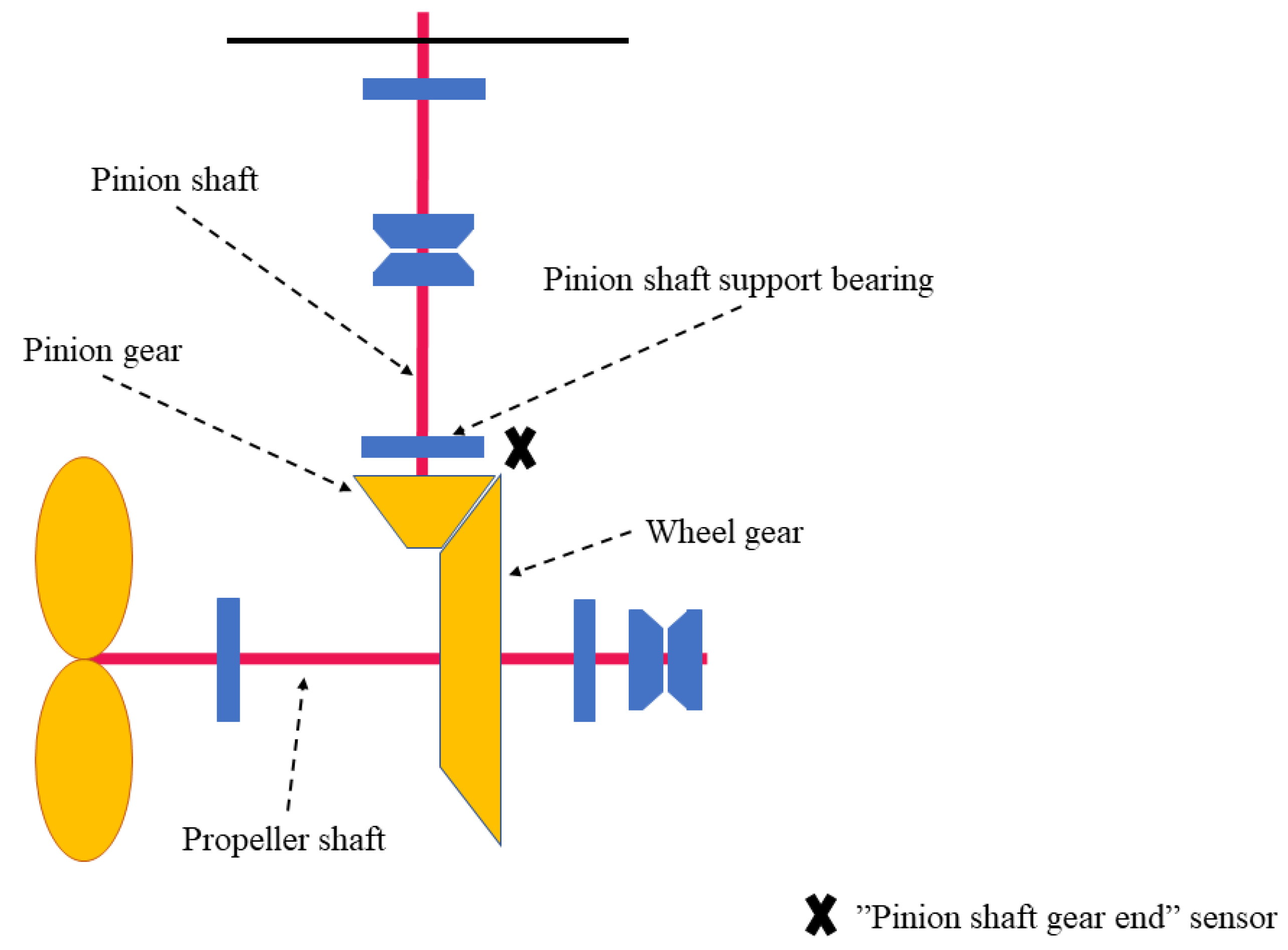
Figure 1. Illustration of azimuth thruster and its main components with approximate placement of accelerometer utilized in this study.
Machines 09 00039 g001
Figure 2. Flowcharts of proposed algorithm: “Measurement data” arrows describe the flow of acceleration signals, their transformations and shaft speed in the algorithm, whereas the dotted arrows for “parameters” describe the flow of parameters defined by user, monitored system or algorithm.
Machines 09 00039 g002
Figure 3. Examples of three signals in data quality control: The signal on top is accepted by all checks, the signal in the middle is rejected in the check for moving mean range, and the signal below is rejected based on the moving mean range and absolute mean.
Machines 09 00039 g003
Figure 4. Amplitude spectra of thruster 1 with shaft speed 346.96 rpm. The upper plot shows a case without reported damage and the lower plot shows a case where the inner race of pinion shaft support bearing was damaged. The median and upper quartile of the amplitudes of 1–10 harmonics of BPFI are shown.
Machines 09 00039 g004
Figure 5. Amplitude spectra of thruster 2 with shaft rotational speed 394.13 rpm. The upper plot shows a case without reported damage and the lower plot shows a case where wear on pinion and wheel gear surfaces was confirmed. The median and upper quartile of 20 amplitudes including the values of 1–4 harmonics and sidebands of gear mesh frequency are shown.
Machines 09 00039 g005
Figure 6. Normal probability plots demonstrating the effect of quantiles in the distribution of residual values. The plot on the left shows the residual of feature no. 4 (median), whereas the upper quartile is shown in the middle and maximum is shown on the right. The parameter H (0 or 1) is the hypothesis result from Kolmogorov-Smirnov test at the 5% significance level.
Machines 09 00039 g006
Figure 7. Illustration of stages in shaft speed range selection using data from thruster 1. First, the samples are sorted based on shaft speed and quantiles are calculated (upper left). The data are then categorized in different ranges based on the quantiles (upper right). Only the ranges with enough samples are taken to the test of normal distribution (lower left). The (lower right) plot shows the number of normal distributed residual sets inside each tested shaft speed range. In this example, only the range no. 26 became selected because it had the widest range from the fourteen overlapping ones that had the highest number of normal distributed sets.
Machines 09 00039 g007
Figure 8. Relation between squared Mahalanobis distance and chi-square cumulative distribution function with three and five degrees of freedom (d). The distances that equal 10%, 5% and 0.1% probabilities are marked in the curves.
Machines 09 00039 g008
Figure 9. “Probabilistic threshold” approach (left) and “two distributions” approach to classification (right).
Machines 09 00039 g009
Figure 10. Generation of training and test sets for outer resampling in nested cross-validation approach. Parameter N stands for the sample size and H is the hypothesis result in Kolmogorov-Smirnov test. Split ratio defines the ratio between training and test set sizes.
Machines 09 00039 g010
Figure 11. Monitoring of thruster 1 by using three different sets of features during a period spanning over 515 days.
Machines 09 00039 g011
Figure 12. Monitoring of thruster 2 by using three different sets of features during a period spanning over 466 days.
Machines 09 00039 g012
Figure 13. Scatter plots of shaft speed with feature values in the data set of thruster 1. The x-axis shows the shaft speed (rpm) and the y-axis shows the feature value. The samples representing “positive class” are taken after the videoscope inspection and “negative class” represents the undamaged condition. The definitions for features no. 1–11 are given in Table 3.
Machines 09 00039 g013
Figure 14. Scatter plots of shaft speed with feature values in the data set of thruster 2. For interpretation, see the caption of Figure 13.
Machines 09 00039 g014
Figure 15. Thruster 1 classification results. The plots from top to bottom show the averages of accuracy, precision, recall and specificity. The results with time domain features, bearing features and gear features are shown by using eight classification methods. The first three methods on the left apply “probabilistic threshold” approach, the fourth method applies “two distributions” approach, and the rest of the results are given by the reference classifiers.
Machines 09 00039 g015
Figure 16. Thruster 2 classification results. For interpretation, see the caption of Figure 15.
Machines 09 00039 g016
Table 1. Kinematic frequencies (Hz) related to 60 rpm shaft speed.
BPFIBPFOBSFFTFGMF
10.84358.15653.36670.429313
Table 2. Parameters used in different processes in the condition monitoring algorithm.
ProcessParameter(s)Example Value
Quality control
(QC parameters)
range limit (g), (1 g ≈ 9.81 m/s2)0.5
absolute mean limit (g)2
Feature extraction
(System parameters)
kinematic frequencies-
sampling rate-
Inference
(Model parameters)
α: probabilistic threshold0.001
n: moving window size5
β0, β1, μ, σ, Σ: regression models, normal distributions-
Speed range selectionminimum sample size60
Filter samplespeed range-
Table 3. Description of features used in this study. Features no. 1–3 are computed from time series, whereas features no. 4–11 are extracted from amplitude spectra based on system-specific definitions.
No.FeatureDetails
1Generalized norm (l10)Order of norm, p = 10
2Ratio of norms (l20/l2)Ratio of high-order norm (p = 20) to low-order norm (p = 2)
3KurtosisIndicator for the tails of probability distribution
4BPFI featureMedian amplitude of 1–10 BPFI harmonics
5BPFO featureMedian amplitude of 1–10 BPFO harmonics
6BSF featureMedian amplitude of {1, 2, 4, 6} BSF harmonics
7BPFI sideband featureMedian amplitude of the nearest sidebands on both sides of BPFI harmonics (20 sidebands altogether, spaced at shaft rotational frequency)
8BSF sideband featureMedian amplitude of the nearest sidebands on both sides of BSF harmonics (8 sidebands altogether, spaced at FTF)
9GMF feature 1Median amplitude of 1–4 GMF harmonics and two nearest sidebands on both sides (20 frequency components altogether)
10GMF feature 2Median amplitude of 1 × GMF and two nearest sidebands on both sides (5 frequency components altogether)
11GMF feature 3Median amplitude of 2 × GMF and two nearest sidebands on both sides (5 frequency components altogether)
Table 4. Correlation coefficients of shaft speed with feature values and residuals computed from the identification data of thruster 1.
No.1234567891011
Features0.750.08−0.140.690.320.670.830.830.710.610.36
Residuals00000000000
Table 5. Parameters for the distributions identified in each shaft speed range.
ParametersDefinitionNumber of Parameters
β0, β1Regression parameters for each feature22
μMeans of each residual set (≈0)11
σStandard deviations of each residual set11
Σ1, Σ2, Σ3Covariance matrices3
Table 6. Classifiers used as reference methods, tested hyperparameter values and Matlab® functions used for classifier training.
ClassifierHyperparameter ValuesMatlab® Function
k-NN‘NumNeighbors’: 1–49, odd numbers onlyfitcknn
LDA‘Gamma’: 0–1, step 0.025
‘Delta’: 0 and 1 × 10−6 × 10x, where x = 0–9, step 1
fitcdiscr
SVM‘KernelScale’: 1 × 10−5 × 10x, where x = 0–10, step 0.4
‘BoxConstraint’: 1 × 10−5 × 10x, where x = 0–10, step 0.4
fitcsvm
AdaBoost M1‘LearnRate’: {0.1, 0.25, 0.5, 0.75, 1}
‘MaxNumSplits’: 10–90, step 10
‘NumLearningCyles’: 10–150, step 20
fitcensemble
Publisher’s Note: MDPI stays neutral with regard to jurisdictional claims in published maps and institutional affiliations.