Transfer of Process References between Machine Tools for Online Tool Condition Monitoring

Abstract

Process and tool condition monitoring systems are a prerequisite for autonomous production. One approach to monitoring individual parts without complex cutting simulations is the transfer of knowledge among similar monitoring scenarios. This paper introduces a novel monitoring method which transfers monitoring limits for process signals between different machine tools. The method calculates monitoring limits statistically from cutting processes carried out on one or more similar machines. The monitoring algorithm aims to detect general process anomalies online. Experiments comprise face-turning operations at five different lathes, four of which were of the same model. Results include the successful transfer of monitoring limits between machines of the same model for the detection of material anomalies. In comparison to an approach based on dynamic time warping (DTW) and density-based spatial clustering of applications with noise (DBSCAN), the new method showed fewer false alarms and higher detection rates. However, for the transfer between different models of machines, the successful application of the new method is limited. This is predominantly due to limitations of the employed process component isolation and differences between machine models in terms of signal properties as well as execution speed.

1. Introduction

Even thorough process preparation of cutting processes does not entirely prevent process failures. Therefore, process and tool condition monitoring systems are a prerequisite for autonomous production [1,2]. The systems evaluate the sensor signals of the machine tool, such as motor currents or signals from external sensors. In series production, process signals from previous parts are available as a reference to perform monitoring. However, when monitoring individual parts, such references are not available. An approach to overcome this issue is a simulation, which generates a reference for the evaluated signal. However, simulations are a simplification of reality. To model processes more realistically, simulations consider an increasing number of effects such as stress, temperature, white layer characteristics of the target surface, and thermomechanical behavior of the material [3]. Consequently, simulations for single parts require an extensive amount of information and usually validation. Therefore, the economic monitoring of single parts with simulations remains challenging.

Another approach that works towards the monitoring of individual parts is to transfer required parameters, references, or models from similar monitoring scenarios. Existing research transfers such monitoring knowledge between similar types of tools [4], between varying cutting parameters [5], or different materials [6]. Little research was found on the transfer of knowledge among different machine tools. For example, Li and Liang [7] use deep learning to detect failure patterns in power signals. Kan et al. [8] describe an approach that quantifies the similarity of signals for entire processes on different machines. While Kan et al. [8] suggest monitoring processes and machine conditions as an application, they do not demonstrate it. Furthermore, the mentioned approaches are only suitable for offline monitoring, which is only sufficient when monitoring tool wear. However, failures such as collision, tool breakage, and chatter require online detection. Rudolf et al. [9], for example, observed a tool breaking within 23 ms due to a collision at a feed of 10 m/min. Consequently, a system designed to detect general anomalies in process and tool condition monitoring requires low reaction times [10]. The authors further emphasize that thresholds for reliable and timely detection are process specific.

This paper proposes and examines a method for timely online detection of general anomalies that uses transferred OK-signal references. The method breaks processes down into frequently occurring geometrical features, e.g., slots or pockets. Then, machine specific characteristics in process signals are compensated. Lastly, monitoring limits for the target machine are calculated statistically from matching OK-references of source machines. The novel aspect is the use of OK-process data of one or more source machines to calculate statistical monitoring limits for the target machine, that are suited for online monitoring. As research exists on process segmentation [11,12,13] and process force reconstruction [3,14], the focus is subsequently on the transfer of knowledge between machines.

The remaining part of the paper is organized as follows: Section 2 introduces the machines and processes examined, as well as the new method. Section 3 characterizes the new method by the example of a face turning operation. Section 3.1 examines monitoring performance when sourcing limits from a single machine only. Further, Section 3.2 investigates the sourcing of monitoring limits from multiple machines by analyzing selected examples.

2. Materials and Methods

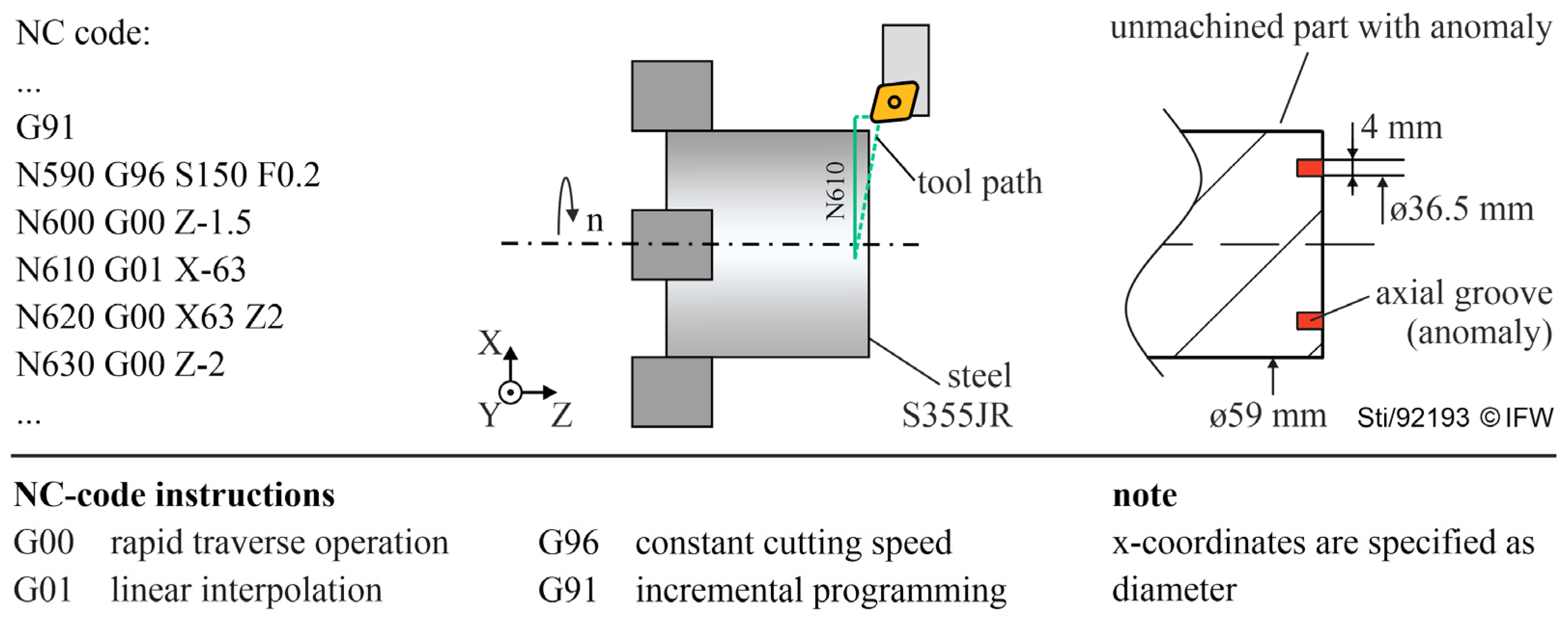
2.1. Experimental Machining

A series of experiments were conducted to examine the new method. Experiments comprised face turning operations under five different process conditions (

Table 1. Cutting conditions.

ID	Process	Parameter
1	face turning	f = 0.2 mm, ap = 1 mm, vc = 250 m/min
2	face turning	f = 0.3 mm, ap = 1 mm, vc = 150 m/min
3	face turning	f = 0.2 mm, ap = 1.5 mm, vc = 150 m/min
4	face turning	f = 0.3 mm, ap = 1.5 mm, vc = 250 m/min
5	face turning	f = 0.25 mm, ap = 1.25 mm, vc = 200 m/min

). NC-code defined the face turning operation with constant cutting speed during the operation (Figure 1). Coated hard metal indexable inserts of the ISO type CNMG 120,408 were used. Tools were sharp with flank wear <100 µm. The workpieces had a length of 110 mm, a diameter of 59 mm and were from mild steel type S355JR (DIN EN10025-2, equivalent to ASTM A 573 M Grade 70). To simulate a process anomaly, an axial groove was machined in the face of the workpiece before the actual face turning operation (Figure 1, right). The groove caused a short drop in the cutting force in a manner partly resembling the behavior occurring when a cutting edge breaks [15].

Experiments were conducted on five different machines, four of which were identical models manufactured in the same year (

Table 2. Examined machine tools.

ID	Type of Lath	Control	Number Examined
A1 to A4	DMG Mori CTX 1250 TC	Sinumerik 840D sl	4
B	DMG Mori CTX beta 800	Sinumerik 840D sl	1

). The identical machines (A1 to A4) had identical equipment (clamping chucks, tool holders, etc.) and were located adjacent to each other. All machines executed the same lines of G-Code that defined the described face-turning operation. Differences in the G-code were limited to the header and the footer of the code, e.g., due to different tool names. The employed drive systems of all machines used ball crew drives.

Signals recorded comprised the actual position of the x-, y-, z-axes as well as the actual speed and command torque of the main spindle. All machines featured a Siemens Sinumerik 840D solution line control. Data were recorded with the built-in “Trace” function of the control at a sample rate of 8 ms.

2.2. Proposed Online Monitoring Method

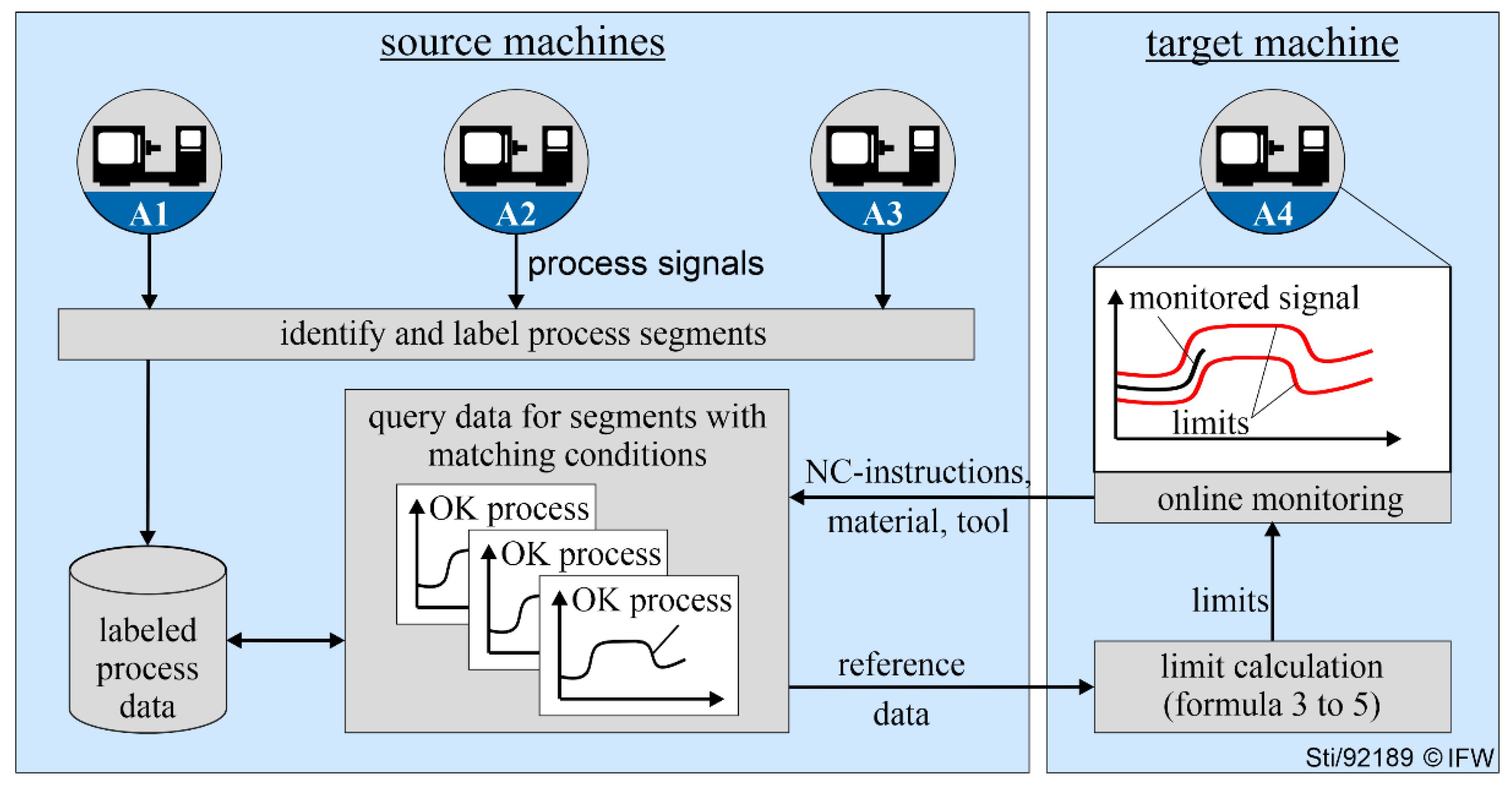
2.2.1. Monitoring with Transferred Knowledge

The source machines provided the OK-processes’ reference data. For the new method to address the monitoring of individual parts without a simulation, these processes were broken down into segments that represented frequently occurring geometrical features, such as slots, pockets and face turning operations. While these segments may not account for the complete machining of an individual part, they were assumed to account for most of it. The segments were then labeled with the type of material, tool and NC-instructions used (Section 2.2.2). To compensate for differences between machines, the process component of a signal was isolated (Section 2.2.3). This followed the idea that a process signal consisted of a component resulting from the process and a component originating from the machine, such as friction or inertia [2]. The segmented, isolated and labeled process signals were then stored for further use.

Figure 2 depicts the research method. A process on the target machine was monitored segment by segment. The approach was separated into offline and online stages. First, NC-instructions were analyzed offline to identify upcoming segments. The source machines provided OK-references that matched the identified segment, material and tool of the target machine. Then, statistical monitoring limits were calculated from the references, as established for series production (Section 2.2.4). The monitoring stage operated online to allow reaction times within the requirements of real time applications. For this, the monitoring procedure compared the actual process signal of the target machine to the calculated monitoring limits (Figure 2). A violation of a monitoring limit triggered an alarm.

The described transfer of references is possible for any signal, such as current signals, torque signals and position control errors. A prerequisite for the new method is that similar processes on different machines lead to similar process signals or signal patterns. As machine-specific properties superimpose these process components, not all signals are equally suitable. With identical processes resulting in identical process forces [2], the process forces provide a mutual characteristic among different machines. If referenced to the tool, the specific kinematics of the machines become secondary.

2.2.2. Process Segmentation

Process segmentation identified the actual start and end of a segment in a process. The employed segmentation utilized the feed speed calculated from the position of the x-, y- and z-axes:

$$fee{d}_{xyz}=\sqrt{{\dot{x}}^2+{\dot{y}}^2+{\dot{z}}^2}$$

(1)

Low-pass filtering the feed $fee{d}_{xyz}$ reduced the impact of signal noise on segmentation. A minimum-order finite impulse response filter was used with a stopband attenuation of 60 dB and a passband frequency of 10 Hz. Segments were then determined, as an interval of the process that ran at a feed typical for cutting operations, such that:

$$50\frac{\mathrm{mm}}{\min }<fee{d}_{xyz}<1000\frac{\mathrm{mm}}{\min }$$

(2)

The identified segments were labeled with information obtained from the NC-code and the machine control, such as the type of segment (slot, face turning, etc.) and geometric properties of the tool. While it is not yet established practice to store information about a workpiece material in machine controls, it is expected to become more common as digital twins establish. Until then, the information might be provided manually.

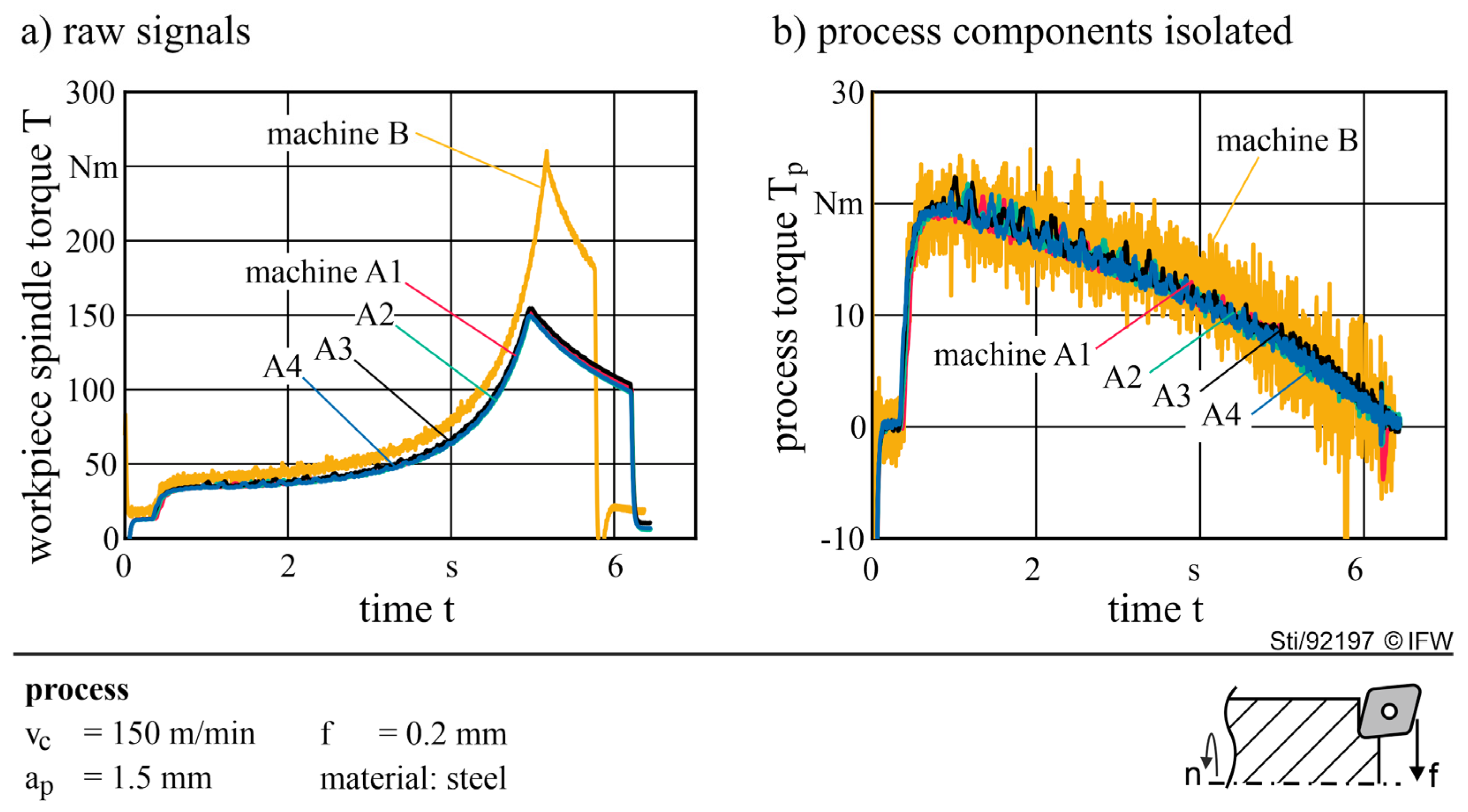
2.2.3. Process Component Isolation

The workpiece spindle torque $T$ was subsequently used for monitoring. It relates to process forces in turning. While process forces are also reflected in the signals of other drives, the workpiece spindle was preferred here, as the examined machines had spindles without gears. This simplified the isolation of the process components when considering multiple machines. Figure 3a depicts the signals of the workpiece spindle torque of all examined machines for cutting condition 1 during a face turning operation in an OK-process. The displayed interval constitutes a single segment as it resulted from the segmentation procedure defined in Section 2.2.2. Differences among the machines arose from different friction, inertia, drive power, and control parameters. The tool entered the material at about 0.4 s. Afterward, the spindles accelerated to maintain cutting speed while the tool moved closer to the center of the workpiece. The cutting process ended at about 6.4 s.

The employed process component isolation compensated the effects of friction and inertia. A lookup table provided the expected friction torque based on the speed and the direction of the spindle rotation. The lookup tables resulted from a dedicated parameterization run, as did the inertia (Figure 4).

Machine A3 behaved differently to the other A machines. A potential cause was a collision suffered by the machine the day before the experiments. The machine and the produced parts were thoroughly checked and assessed to be within required tolerances. Experiments were carried out on a machine cleared for regular production.

The compensation of inertia effects was based on the empirically determined inertia and spindle acceleration. Figure 3b depicts the process component T_p isolated from the workpiece spindle torque. The isolation had limited usability at the beginning of the segment, where boundary effects impaired the accuracy of isolation. Another inaccuracy was the drop in the process component of machine B at about 5.7 s.

2.2.4. Calculating Monitoring Limits

Calculation of monitoring limits required data of multiple OK-processes as a reference. Let the time series $X_k=x_{k,1},\dots ,x_{k,n}$ represent the signal of the processes $k=1,\dots ,K$ at the sample points $i=1,\dots ,n$. Upper and lower monitoring limits were determined separately for each sample point $i$ at a time. First, an upper and a lower envelope $H$ were determined for each reference process. The envelope accounted for temporal variance in process signals. The width of the envelope and thereby the tolerance to temporal variation was determined by the parameter $Q$:

$$\begin{gathered} H_{k,high}\left(i\right)=maximum\left(x_{k, i-Q}, \dots , x_{k,i+Q}\right) \\ {H}_{k,low}\left(i\right)=minimum\left(x_{k,i-Q}, \dots , x_{k,i+Q}\right) \end{gathered}$$

(3)

Variations in the signal amplitude across the reference processes were considered statistically by calculating an upper and lower monitoring limit $L$ from the corresponding envelopes of all reference processes

$$\begin{gathered} L_{high}\left(i\right)={\overline{h}}_{high}\left(i\right)+C_{safty}·s\left(H_{high}\left(i\right)\right) \\ {L}_{low}\left(i\right)={\overline{h}}_{low}\left(i\right)-C_{safty}·s\left(H_{low}\left(i\right)\right) \end{gathered}$$

(4)

where $\overline{h}\left(i\right)$ is the average across all reference processes $k=1,\dots ,K$ for a sample point $i$. The parameter C_safety defines the distance from the average to the limits. Further, $s\left(e\left(i\right)\right)$ is the standard deviation across all reference processes $k$ as calculated by:

$$s\left(h\left(i\right)\right)=\frac{1}{K-1}\sqrt{{{\displaystyle \sum }}_{k=1}^K{\left(h_k\left(i\right)-\overline{h}\left(i\right)\right)}^2}$$

(5)

The standard deviation, $s$, modeled variations that occurred in the underlying data. That included, for example, batch variations in materials and tools, the tool wear or random measurement errors from data acquisition. Calculating the standard deviation from data of multiple machines considered variations among machines, such as systematic measurement errors or varying precision in process component isolation. The parameter $C_{safty}$ defined by how many standard deviations a signal amplitude must deviate from the mean $\overline{h}$ to be considered an anomaly. As the parameters $C_{safty}$ and $Q$ decreased, monitoring became more sensitive to failures, however, the false alarm rate increased as well. A used compromise for stable machining processes in series production was, for example, $C_{safty}$ = 6 and $Q$ equivalent to 30 ms.

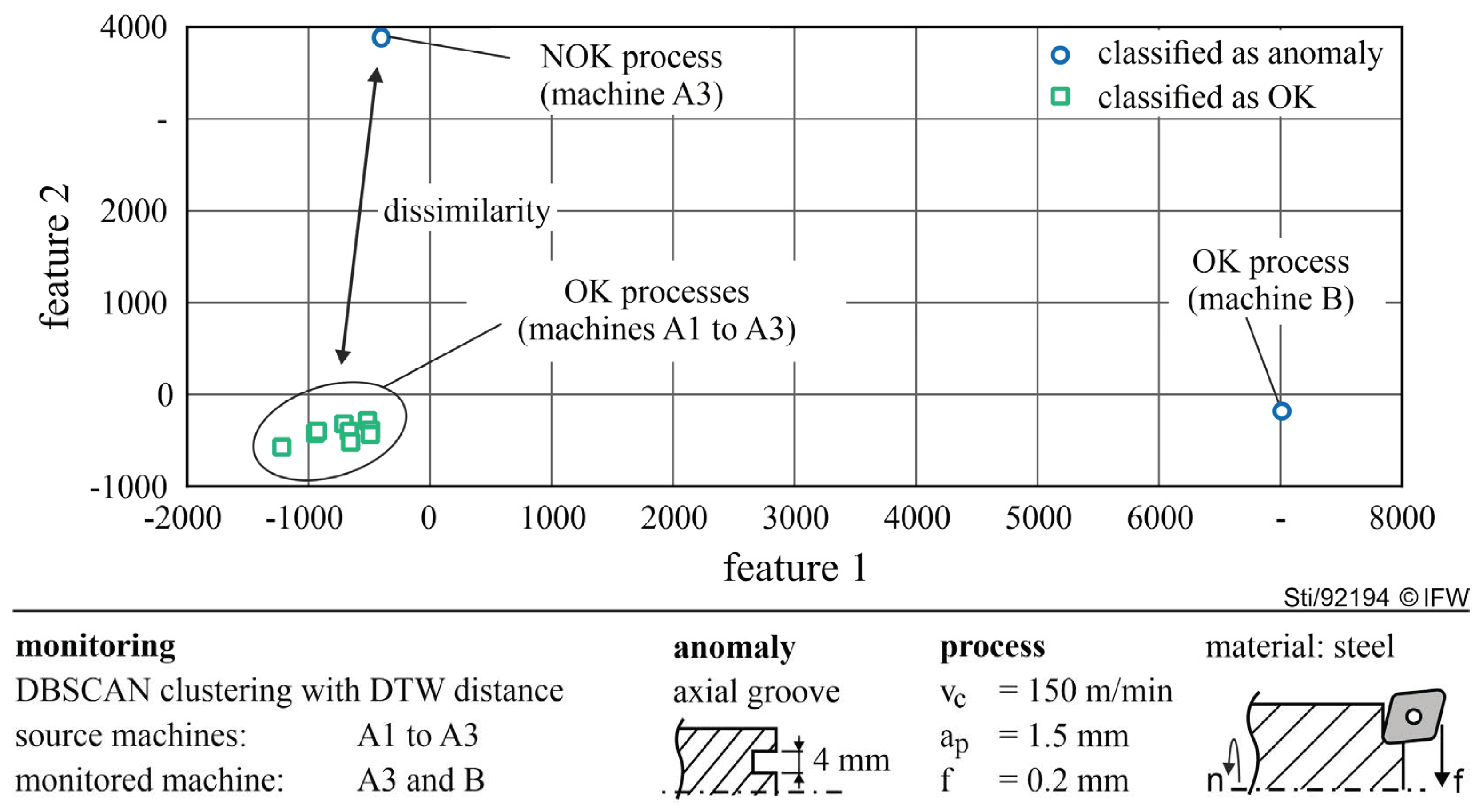
2.3. DTW-Based Anomaly Detection as a Performance Reference

To better evaluate the performance of the new online monitoring method, its results were compared with those of an offline anomaly detection. As recommended by Kan et al. [8] for the monitoring of machines, the employed anomaly detection used dynamic time warping (DTW) to quantify the similarity of two signals. DTW as a measure tolerates temporal differences between otherwise similar signals. It was therefore expected to be more robust against machine dissimilarities than the proposed method, thereby providing a performance reference. The offline anomaly detection was performed by: (I) quantifying the dissimilarity of signal segments pairwise using DTW, and (II) using these dissimilarities to classify the process on the target machine with density-based spatial clustering of applications with noise (DBSCAN). Tuning of hyper parameters for DBSCAN followed [16]. Results were generated with Matlab.

3. Results and Discussion

Robust and yet sensitive monitoring of anomalies requires information about the characteristics of an OK-process. Instead of simulating the process, this reference was subsequently sourced from machines that were similar to the monitored machine. One or more source machines provided nine signals of OK-processes in total. Limits for monitoring were then calculated from the references (Formulas (3)–(5)). Unless stated otherwise, the reported monitoring limits were based on parameters that were suited for series production ($C_{safty}$ = 6 and $Q$ equivalent to 30 ms). A single process segment, a face turning operation, was examined. The subsequent sections investigate the influence of different source machines and preprocessing steps on false alarm and detection rates.

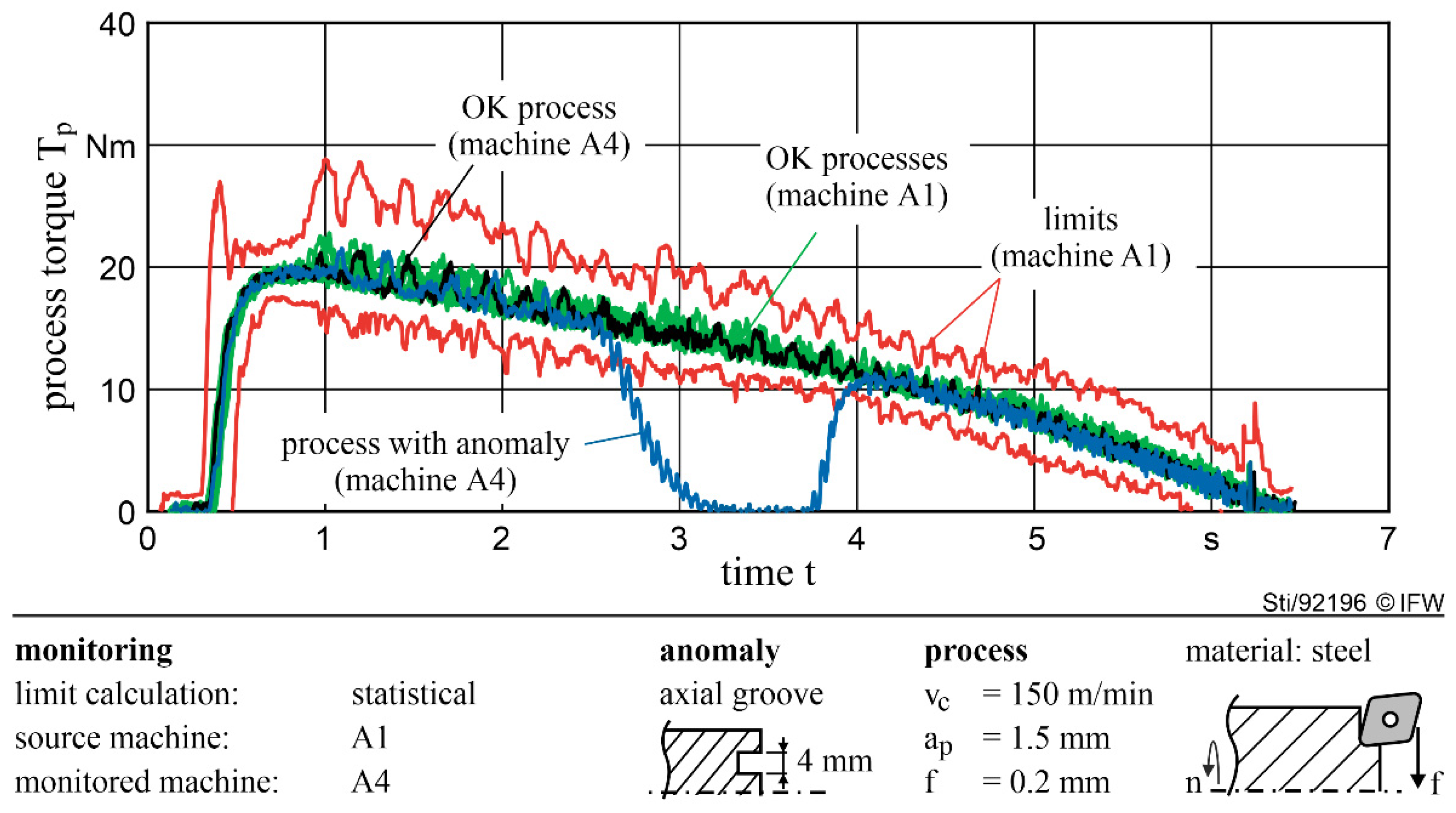
3.1. Sourcing Monitoring Limits from a Single Machine

A single source machine provided all nine OK-signals for monitoring limit calculation. On the target machine a process with anomaly (NOK-condition) was monitored to assess the sensitivity of the monitoring limits. Additionally, an OK-process was monitored to check for false alarms. Each of the five cutting conditions was examined separately. Consequently, for any pair of machines, a maximum of five failures could be detected and a maximum of five false alarms could occur.

Figure 5 depicts the results of machine A1 as a source with machine A4 as a monitoring target for cutting condition 2. The anomaly (axial groove) was successfully detected in the NOK-process and no false alarms occurred during the monitoring of the OK-process. Results were identical for the other four cutting conditions. Consequently, the transfer of monitoring limits from machine A1 to A4 was considered successful.

Figure 6 summarizes detected anomalies and occurred false alarms across all cutting conditions (Table 1) for any pair of machines. Overall, 125 scenarios were examined. An example was the transfer between machines A1 and A4 as described in the preceding paragraph (Figure 6a; pair A1, A4). The diagonal of a matrix represents a machine monitoring itself with its own OK-references, as it would in series production. The corresponding 25 scenarios were excluded from the analysis, leaving 100 scenarios that represented a transfer situation. Parts (a) to (f) of Figure 6 assess different approaches and different parameters.

Figure 6a shows the results of the new approach with monitoring parameters as in series production ($C_{safty}$ = 6 and $Q$ equivalent to 30 ms). In total, 97% of anomalies were detected in NOK-processes and false alarms occurred in 67% of monitored OK-processes. Results varied among pairs of source-target machines. For example, monitoring limits transferred between machines A1 and A4 detected all anomalies without false alarms. The transfer worked either way. Machine B was able to donate monitoring limits to any machine and only a single false alarm occurred while reaching a detection rate of 72%, on average. In contrast, no monitoring limits could be transferred to machine B as a target, without false alarms.

A cause for false alarms was differences in signal noise. While the signal noise was not significantly different among the machines A1 to A4, the noise was higher in the signals of machine B (Figure 7). Consequently, monitoring limits calculated from machine B were wider, causing fewer false alarms at the cost of impaired sensitivity to anomalies. Possible causes for the higher noise of machine B were sensor characteristics, dynamic characteristics of the machine, and unnoticed faults, e.g., in a bearing. Consequently, these aspects might serve as an indicator for the success of a transfer.

Additionally, the employed process force isolation caused false alarms at about 0 s to 0.25 s and at about 2.2 s, where it falsely created a signal valley for machine B. A more precise process component isolation would consequently increase the transferability of monitoring limits. In addition, a more sophisticated process component isolation might compensate disturbances in process signals that arise from the dynamic characteristics of a machine.

Further, a difference in signal length is noticeable in Figure 7. The signal of machine B is shorter than the signals of machines A1 to A4 (at 2.8 s). This indicates that a difference in tool contact time existed between machines that is relevant from the perspective of online monitoring.

Using wider monitoring limits ($C_{safty}$ = 12 and $Q$ equivalent to 60 ms) with the new approach reduced false alarms to 35% (Figure 6b). With fewer false alarms, however, detection rates decreased, from initially 97%, to 93%. From a perspective of applicability, it was a beneficial tradeoff to reduce false alarms to 35% while accepting a decreased detection rate of 93%. Despite the improvement, the false alarm rate is still too high for industrial application. As false alarms are predominantly caused by certain pairs of machines, a selection mechanism for suited machines has the potential to further improve results.

Figure 6c,d depict the new approach, but without process component isolation (with signals as in Figure 3a). The most prominent consequence of omitting the process component isolation is an increase in false alarms, e.g., false alarms occurred in 98% of scenarios in Figure 6c versus 67% in Figure 6a. Widening monitoring limits (to $C_{safty}$ = 12 and $Q$ equivalent to 60 ms) reduced false alarms to 83% (Figure 6d). This highlights the importance of the process component isolation within the proposed method.

When comparing the proposed method (Figure 6a,b) to the DTW-based reference method (Figure 6f), the proposed method yielded higher detection rates (93% versus 83%) and fewer false alarms (35% versus 69%). Both methods benefited from the isolation of process components, in that false alarm rates decreased. Process component isolation enabled the proposed method to source monitoring limits from machine B with only one false alarm occurring on the monitored machines A1–4 (Figure 6a). However, monitoring of machine B resulted in the maximum number of false alarms possible. This asymmetry was not observed for the DTW-based reference method, as machine B remained unsuited as a source or as a target due to false alarms occurring in all of the evaluated scenarios.

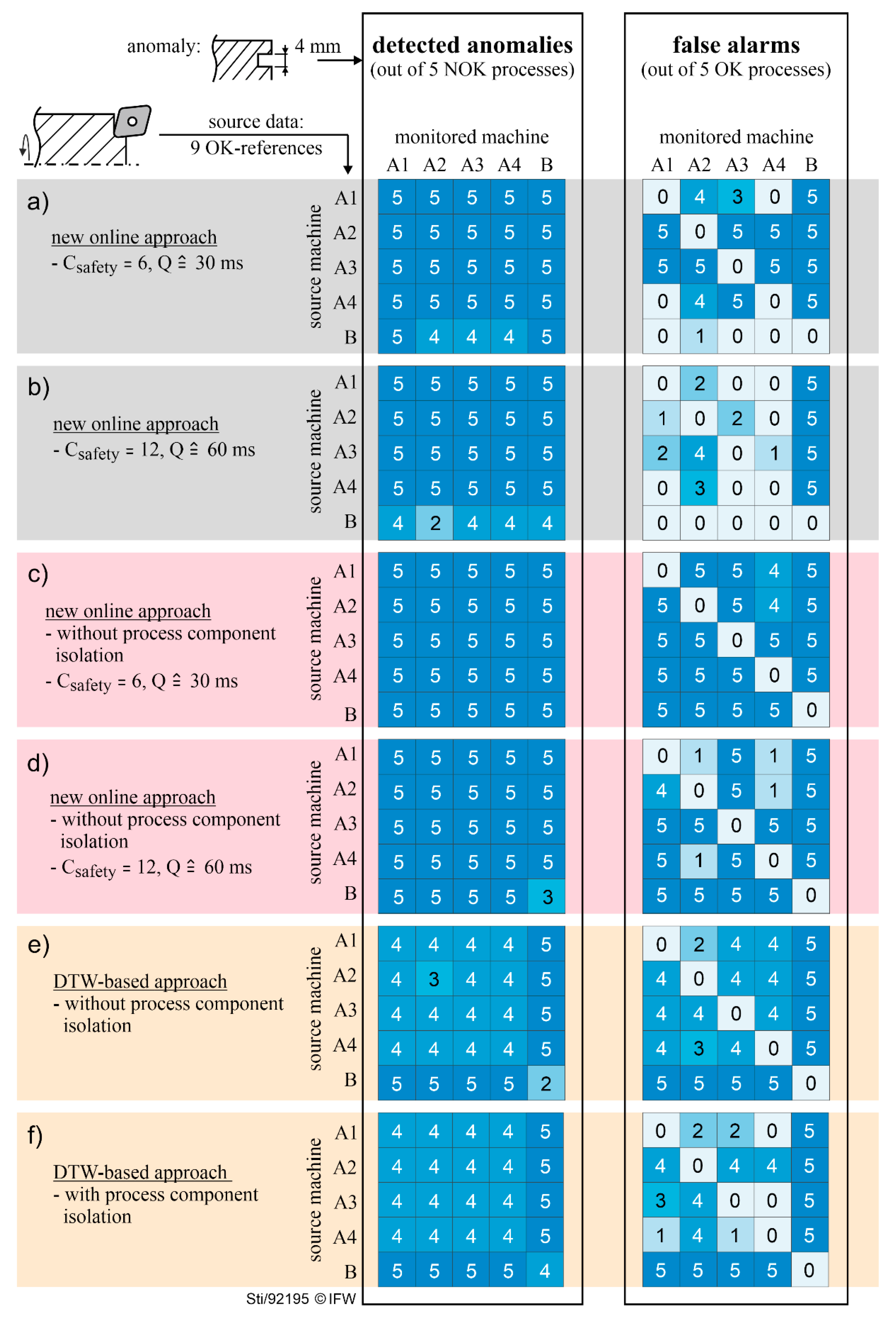
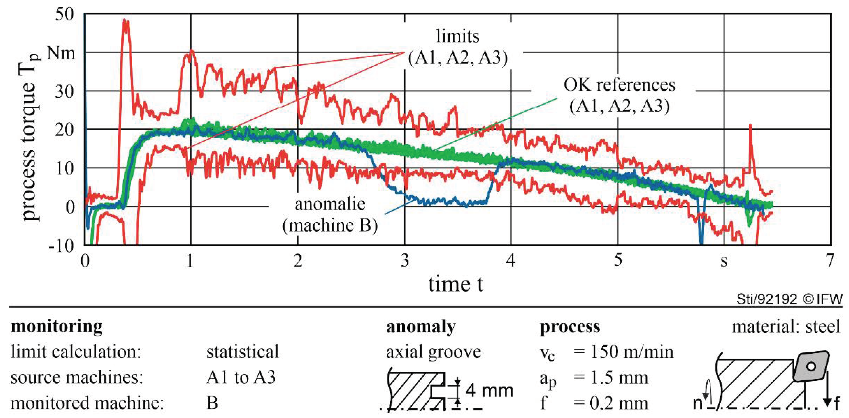
3.2. Sourcing Monitoring Limits from Multiple Machines

To better account for differences among machines, this section calculates statistical monitoring limits from reference processes of multiple machines. Three source machines contributed three reference processes each, resulting in a total of nine OK-references available for monitoring limit calculation. The evaluation considered process condition 3 only to demonstrate expected differences as an example.

3.2.1. Transfer between Multiple Machines of the Same Model with Identical Equipment

The new approach successfully sourced monitoring limits from three machines and transferred them to a target machine for any constellations of type A machines ($C_{safty}$ = 6 and $Q$ equivalent to 30 ms). No false alarms occurred and the failure was detected in all cases.

Without the process component isolation, the transfer of monitoring limits was possible when machine A3 was among the source machines. Figure 8a depicts such a scenario with machine A4 as a monitoring target. The abnormal process was detected and no false alarms occurred during the monitoring. Monitoring limits were generally wider when sourced from a single machine. This resulted from a higher variation between signals, which was predominantly introduced by machine A3. Machine A3 was the most different machine in the group of type A machines from the perspective of idle torque. Consequently, machine A3 was unsuited as a monitoring target. Monitoring machine A3 resulted in frequent false alarms, e.g., five false alarms were triggered during the run depicted in Figure 8b.

The DTW-based reference method also classified the processes with and without anomalies correctly for any constellation of type A machines. The process component isolation was not required, which is an advantage over the proposed method.

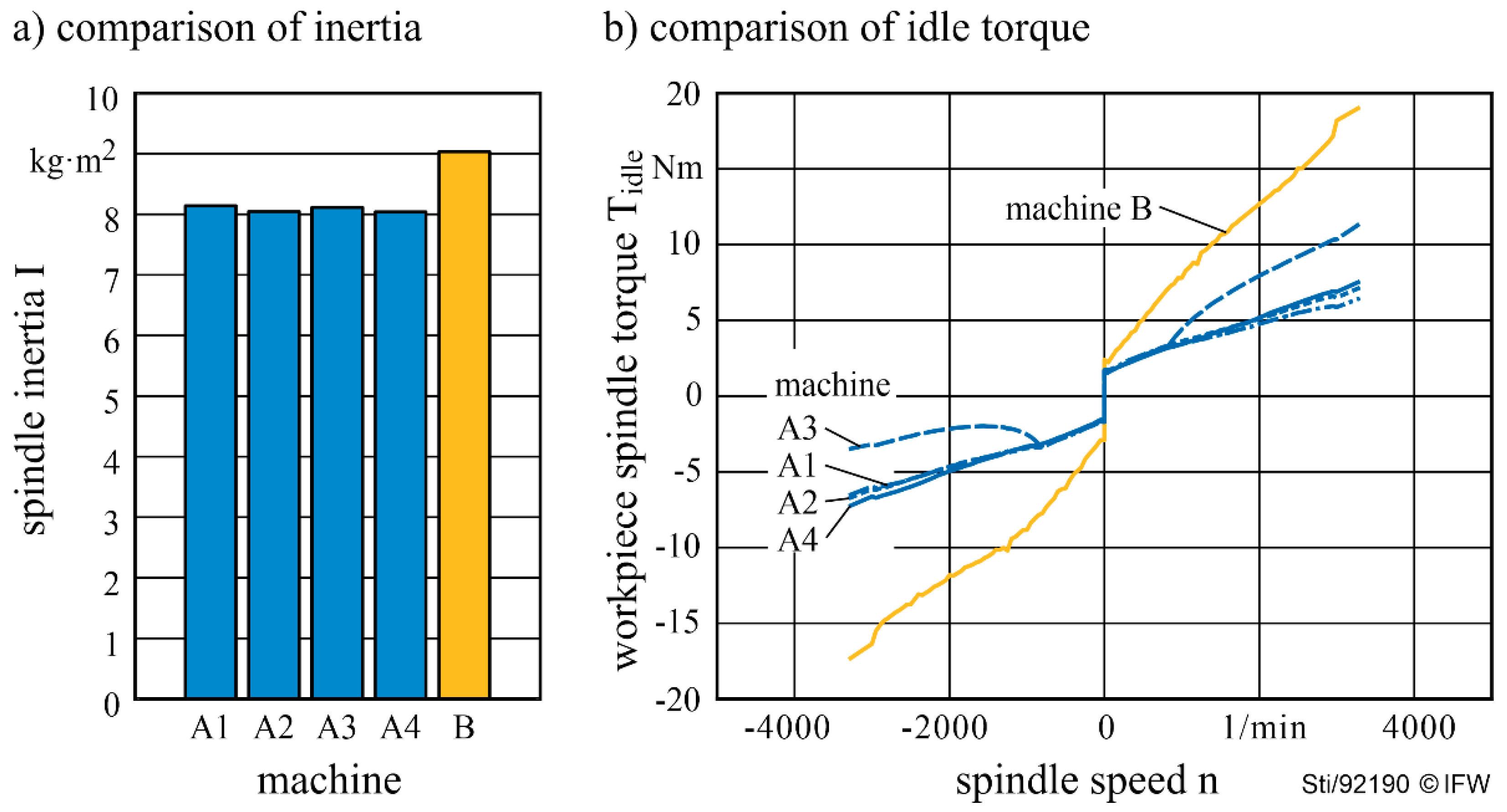
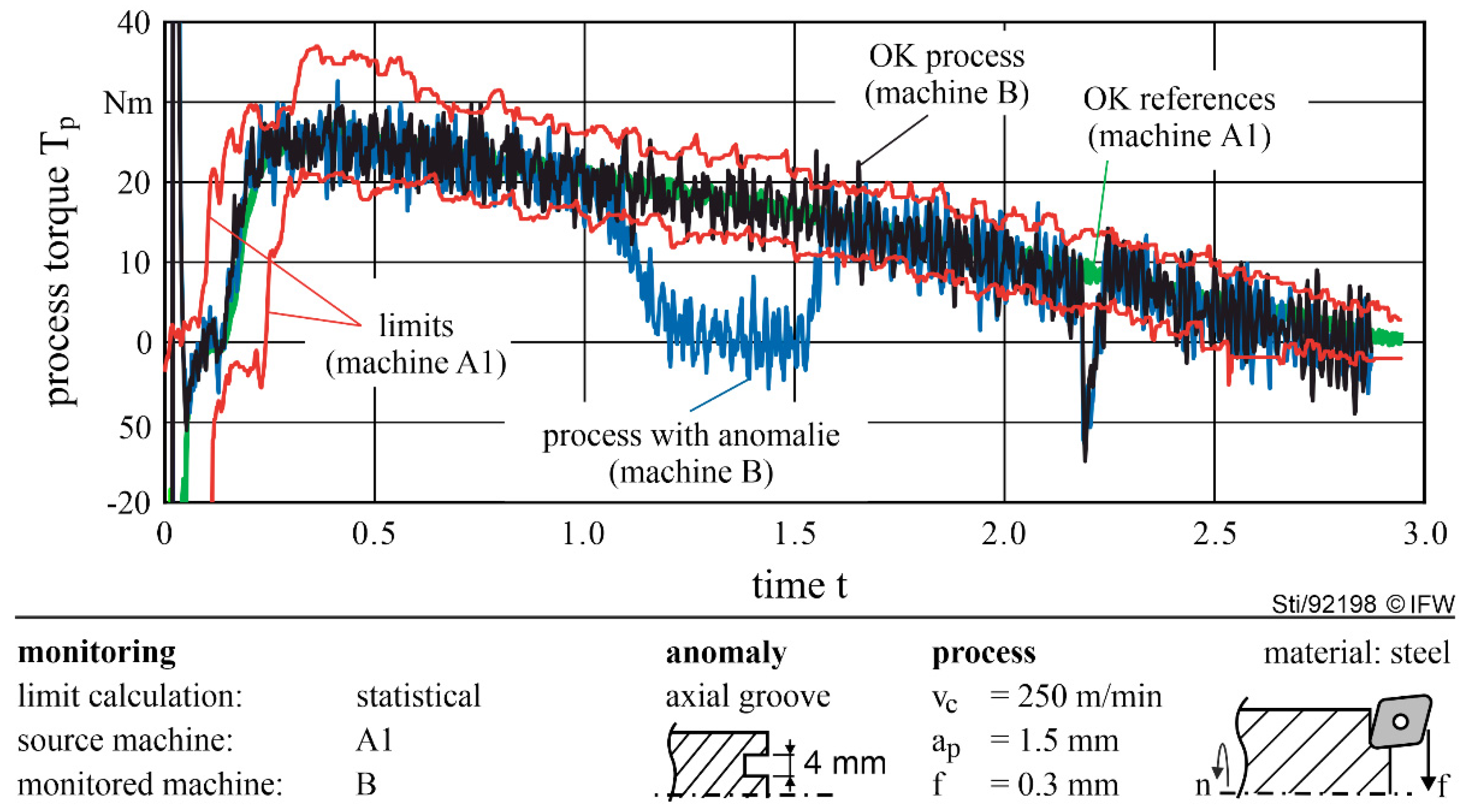
3.2.2. Transfer between Multiple Machines of Different Models

For the different models of machines, no monitoring was possible with the proposed method. More than 50 false alarms occurred within a single face turning operation. This was due to the higher signal variation of machine B compared with the type A machines (as in Figure 7). Smoothing the signal of machine B (running mean, window size 20 samples) reduced false alarms to a total of two: one at the very beginning of the segment and one at about 5.8 s (Figure 9). The reason for both false alarms was an insufficient process component isolation.

It was further observed that type A machines required about 80 ms longer to execute the face turning operation than machine B. This became an issue when transferring monitoring limits from machine B to a type A machine. In this case, no monitoring limits were available towards the end of the face turning operation. A possible solution is the extrapolation of monitoring limits. In addition, the occupied bandwidth of the signals differed among the machine tool models. Consequently, failures that only reflect in higher frequencies of the signals might be monitored on one type of machine, but not on another.

With the DTW-based reference method, no monitoring was possible (transfer A1–3 to B), despite isolating process components. While the approach detected the NOK-process, it also classified the OK-processes on the target machine falsely as anomalies. Figure 10 shows the classification results and visualizes the dissimilarity of the process segments as quantified with DTW and mapped via multidimensional scaling. The OK-processes of the source machines were grouped in a cluster. A NOK-process of a source machine, as a reference, was detected as an anomaly due to its distance from the OK-cluster. The OK-process of the target machine had a greater distance from the OK-cluster than the NOK-process of a source machine. Consequently, it was falsely classified as an anomaly. The NOK-process of the target machine was omitted from Figure 10 as its high distance from the OK-cluster diminished readability of the figure.

4. Conclusions

This paper proposed a new method to enable online detection of anomalies in machining without process simulations. The method transfered signal references of OK-processes from similar machines using three mechanisms: First, processes were broken down into standardized geometrical features, e.g., slots or pockets, to increase chances of finding a matching OK-reference. Second, process components in signals were isolated to increase the similarity of signals across machines. Third, monitoring limits for the target machine were calculated statistically segment by segment from matching OK-references of other machines.

Experiments and the analysis focused on the influence of different machines on the detection rate and false alarm rate. The proposed method successfully transferred OK-references for a face turning operation between machines of the same model. The proposed method outperformed a machine learning approach based on dynamic time warping and density-based spatial clustering of applications with noise. The transferability of OK-references depended on the exact pair of machines and the transfer direction. For selected machines of the same model, transfer was possible without any false alarms. When transferring among machines of different models, the success depended on the direction of transfer. The transfer was impaired by signals having different variances, by temporal differences in machining time and by insufficient reconstruction of process torque.

The observed temporal differences in machining and signal properties pose challenges beyond the scope of process force isolation and should be investigated. Further research should evaluate these differences and their effect on monitoring with transferred knowledge. Additionally, the proposed method should be extended to include a mechanism that selects suited machines beforehand. This requires a metric to quantify the similarity of machines and a concept to define when similarity is sufficient to allow the transfer of OK-references. In addition, the interactions of sourcing references from various machines and splitting processes into standard geometrical features requires further research.

References

1. Salgado, D.R.; Cambero, I.; Herrera Olivenza, J.M.; García Sanz-Calcedo, J.; Núnez López, P.J.; García Plaza, E. Tool wear estimation for different workpiece materials using the same monitoring system. Procedia Eng. 2013, 63, 608–615. [Google Scholar] [CrossRef] [Green Version]
2. Lee, J.Y.; Shin, Y.J.; Kim, M.-S.; Kim, E.S.; Yoon, H.S.; Kim, S.Y.; Yoon, Y.C.; Ahn, S.H.; Min, S. A Simplified Machine-Tool Power-Consumption Measurement Procedure and Methodology for Estimating Total Energy Consumption. J. Manuf. Sci. Eng. 2016, 138, 51004. [Google Scholar] [CrossRef]
3. Altintas, Y.; Kersting, P.; Biermann, D.; Budak, E.; Denkena, B.; Lazoglu, I. Virtual process systems for part machining operations. CIRP Ann.-Manuf. Technol. 2014, 63, 585–605. [Google Scholar] [CrossRef]
4. Hassan, M.; Damir, A.; Attia, H.; Thomson, V. Benchmarking of Pattern Recognition Techniques for Online Tool Wear Detection. Procedia CIRP 2018, 72, 1451–1456. [Google Scholar] [CrossRef]
5. Wang, P.; Liu, Z.; Gao, R.X.; Guo, Y. Heterogeneous data-driven hybrid machine learning for tool condition prognosis. CIRP Ann.-Manuf. Technol. 2019, 68, 455–458. [Google Scholar] [CrossRef]
6. Cai, W.; Zhang, W.; Hu, X.; Liu, Y. A hybrid information model based on long short-term memory network for tool condition monitoring. J. Intell. Manuf. 2020, 31, 1497–1510. [Google Scholar] [CrossRef]
7. Li, W.D.; Liang, Y.C. Deep transfer learing based diagnosis for machining process lifecycle. Procedia CIRP 2020, 90, 642–647. [Google Scholar] [CrossRef]
8. Kan, C.; Yang, H.; Kumara, S. Parallel computing and network analytics for fast Industrial Internet-of-Things (IIoT) machine information processing and condition monitoring. J. Manuf. Syst. 2018, 46, 282–293. [Google Scholar] [CrossRef]
9. Rudlf, T.; Brecher, C.; Possel-Dolken, F. Contact-based collision detection—A new approach to avoid hard collision in machine tools. In Proceedings of the International Conference on Smart Machining Systems, Gaithersburg, MD, USA, 13–15 March 2007. [Google Scholar]
10. Abele, E.; Brecher, C.; Gsell, S.C.; Hassis, A.; Korff, D. Steps towards a protection system for machine tool main spindles against crash-caused damages. Prod. Eng. 2012, 6, 631–642. [Google Scholar] [CrossRef]
11. Denkena, B.; Fischer, R.; Euhus, D.; Neff, T. Simulation based process monitoring for single item production without machine external sensors. Procedia Technol. 2014, 15, 341–348. [Google Scholar] [CrossRef] [Green Version]
12. Denkena, B.; Dahlmann, D.; Damm, J. Self-adjusting Process Monitoring System in Series Production. Procedia CIRP 2015, 33, 233–238. [Google Scholar] [CrossRef] [Green Version]
13. Bombinski, A.; Blazejak, K.; Nejman, M.; Jemielniak, K. Sensor signal segmentation for tool condtion monitoring. Procedia CIRP 2016, 46, 155–160. [Google Scholar] [CrossRef] [Green Version]
14. Bergmann, B.; Witt, M. Feeling machine for material-specific machining. CIRP Ann.-Manuf. Technol. 2020, 63, 353–356. [Google Scholar] [CrossRef]
15. Denkena, B.; Bergmann, B.; Witt, M. Feeling Machine for Process Monitoring of Turning Hybrid Solid Components. Metals 2020, 10, 930. [Google Scholar] [CrossRef]
16. Ester, M.; Kriegel, H.-P.; Sander, J.; Xu, X. A density-based algorithm for discovering clusters in large spatial databases with noise. In Proceedings of the Second International Conference on Knowledge Discovery in Databases and Data Mining; AAAI Press: Portland, OR, USA, 1996; pp. 226–231. [Google Scholar]
Figure 1. Experimental machining.
Machines 09 00282 g001
Figure 2. Scheme for online monitoring with transferred knowledge.
Machines 09 00282 g002
Figure 3. Comparison of (a) raw signals as recorded from the machines and (b) process components isolated from raw signals. The depicted interval constitutes a single segment with a face turning operation in OK-condition.
Machines 09 00282 g003
Figure 4. Comparison of parameters used to compensate (a) inertia and (b) idle torque on lathes.
Machines 09 00282 g004
Figure 5. Successful detection of an abnormal process on the target machine using statistical monitoring limits sourced from a similar machine. No false alarms occurred.
Machines 09 00282 g005
Figure 6. Detected anomalies and occurred false alarms summarized for all cutting conditions. Results depicted for individual pairs of source-target machines. (ad): the proposed online method under varying input data and parameters. (e,f): the offline approach as a reference.
Machines 09 00282 g006
Figure 7. Monitoring of an OK-process and a process with anomaly using statistical monitoring limits calculated from another machine. The difference in signal noise impaired monitoring and caused false alarms.
Machines 09 00282 g007
Figure 8. Transfer of monitoring limits among machines of the same model and without process component isolation. (a) Anomaly detected and no false alarms with machine A4 as a target. (b) Anomaly detected, but several false alarms with machine A3 as a monitoring target.
Machines 09 00282 g008
Figure 9. Transfer of monitoring limits among machines of different models.
Machines 09 00282 g009
Figure 10. Similarity of signals for face turning operations on different machines visualized via multidimensional scaling. The DBSCAN algorithm falsely classifies the OK-process of machine B as an anomaly.
Machines 09 00282 g010