Article

Kinematic Analysis and Parameter Measurement for Multi-Axis Laser Engraving Machine Tools

1
School of Mechanical Engineering and Automation, Beihang University, Beijing 100191, China
2
Jiangxi Research Institute of Beihang University, Nanchang 330096, China
3
Research and Application Center of Advanced CNC Machining Technology, State Administration of Science, Technology and Industry for National Defence, Beijing 100191, China
*
Author to whom correspondence should be addressed.
Machines 2021, 9(10), 237; https://doi.org/10.3390/machines9100237
Submission received: 31 August 2021 / Revised: 1 October 2021 / Accepted: 13 October 2021 / Published: 16 October 2021
(This article belongs to the Special Issue Robotic Machine Tools)

Abstract

:
Multi-axis Laser Engraving Machine Tools (LEMT) are widely used in precision processing of parts with complex surface. The accuracy of kinematic model and parameter measurement are the key factors determining the processing quality of LEMT. In this paper, a kinematic model of multi-axis LEMT was established based on Homogeneous Transformation Matrix (HTM). Two types of unknown parameters, linkage parameters and positioning parameters, were measured in the presented model. Taking advantage of the characteristics of laser processing, this paper proposed a rapid measurement method of linkage parameters by combining the machine tool motion with the laser marking action. For positioning parameters, this study proposed a non-contact measurement method based on structured light scanner, which can obtain the translation values and the rotation values from the Workpiece Coordinate System (WCS) to the Basic Coordinate System (BCS) simultaneously. After the measurement of two kinds of parameters of a multi-axis LEMT was completed, the processing of a spatial curve was performed and the average contour error was controlled at 15.1 μ m, which is sufficient to meet the project requirements.

1. Introduction

In recent years, laser engraving has become an important technology of microstructure manufacturing and multi-axis laser engraving machine tools (LEMT) have attracted increasing interest as a result [1]. Higher accuracy of multi-axis LEMT is a critical requirement to meet the challenges of manufacturing precision components. To achieve high-precision control of the laser focus position, it is essential to establish an accurate kinematic model of the machine tool. At the same time, the ability to accurately and quickly measure the unknown parameters in the model is an important step to achieve high-quality and high-efficiency laser processing [2,3].
The kinematic modeling of multi-axis machine tools has always been a hot topic, and many scholars have proposed different modeling approaches. Multi-body theory is one of the most widely applied methods to establish the kinematic model of machine tools, and it can be used to analyze the kinematics and dynamics performance of the machine tool simultaneously [4]. In Multi-body theory, the dynamic equations for each component obtained by handling each component of the machine tool as an independent substructure, and the constraint equations for the system can then be determined based on the constraint conditions of the substructures [5]. Another well-established modeling method is Denavit–Hartenberg (D–H) transformation, which trades a multi-axis machine tool as a system of several links, with each link connected to its neighboring counterparts by two joint elements. In D–H transformation, three translation parameters are required to specify the link position and two angular parameters are necessary to define its orientation [6,7]. Screw theory was applied to the model of multi-axis machine tools in recent years, which can be used to build a general kinematics model for all possible configurations of five-axis machine tools. Screw theory can give complete inverse kinematics solutions for both rotary and translational motions by linking all the coordinates to the base coordinate system [8]. Based on screw theory, the geometric errors of the five-axis machine tool was measured, which can improve the machining accuracy after compensation [9].
All the above-mentioned methods can describe the movement of different machine tools, but their calculations are usually complex and difficult to understand. Homogeneous transfer matrix (HTM) is a general method of object kinematics description, which was initially used in the model of robotics. In the HTM method, each moving component is considered to be a rigid body, the motion relationship between each component can be represented by a 4 × 4 coordinate transformation matrix. The advantage of the HTM method is that the relationship between two moving components can be changed by a straightforward modification of the corresponding variables in the matrix with simple calculations [10]. The HTM method has been used to establish kinematics models of five-axis machine tool with various structural forms, and analysis methods of geometric errors, or even “error map” of machine tools have been developed by several researchers [11,12]. The HTM method is accurate, universal and easy to understand, therefore, this paper chose the HTM method to establish the kinematic model of multi-axis LEMT.
In addition to the establishment of the kinematic model of the multi-axis machine tool, two types of parameters need to be measured to ensure the accuracy of the model: linkage parameters and positioning parameters. Linkage parameters are also called position independent geometric parameters. These parameters determine the accuracy of multi-axis linkage transformation and are caused by assembly errors between components [13]. The positioning parameters are also called the workpiece origin localization, which represents the position relationship between programming coordinate system of the workpiece and basic coordinate system of machine tool after the workpiece is clamped [14]. Both the linkage and positioning parameters of the multi-axis LEMT are detailed in Section 2.
For the measurement of linkage parameters, the traditional methods always depend on high-precision instruments. Some scholars moved the machine tools according to a certain trajectory, and used a laser interferometer to collect the deviation between the command value and the actual value to calculate the linkage parameters [15]. Some other scholars used ball-bars to measure the linkage parameters of the five-axis machine tool, the accuracy has been improved without changing the hardware of the machine tools [16]. Probe is another instrument used in measurement, several errors of the rotary axis can be measured by the contact probe [13]. The above-mentioned measurement methods need to rely on instruments such as laser interferometer, ball-bar, probe, etc., which are usually expensive and complicated to operate, and sometimes are not applicable in laser processing.
For the measurement of positioning parameters, the traditional method in the field of mechanical processing is to contact the tools and the workpiece to obtain the positioning parameters [17]. But the traditional method is not suitable for laser processing because there are no tools or benchmark to make contact with the workpiece [18,19]. To overcome this limitation, some scholars use non-contact measurement methods to obtain positioning parameters. They used CCD cameras to take a plan view of the workpiece, and obtain the workpiece origin localization based on image analysis [14,20]. However, the CCD cameras can only measure the translation values from the workpiece coordinate system to the machine tool coordinate system, and cannot fulfill the measurement of rotation values, whose influences on the machining accuracy should not be ignored.
This paper is structured as follows: first, the kinematic model of multi-axis LEMT was established based on the HTM method (in Section 2), and the linkage parameters and positioning parameters in the model are measured (in Section 3). In the process of linkage parameter measurement, this paper proposed a rapid method by combining the machine tool motion with the laser marking action, which can improve the efficiency of measurement. As for positioning parameters, this study proposed a non-contact measurement method using structured light scanner, which can obtain the translation values and rotation values from the workpiece coordinate system (WCS) to the basic coordinate system (BCS) at the same time. Finally, the measurement of two kinds of parameters of a multi-axes LEMT is completed, and the processing of a spatial curve is taken as an example to verify the accuracy of the measured values (in Section 4).

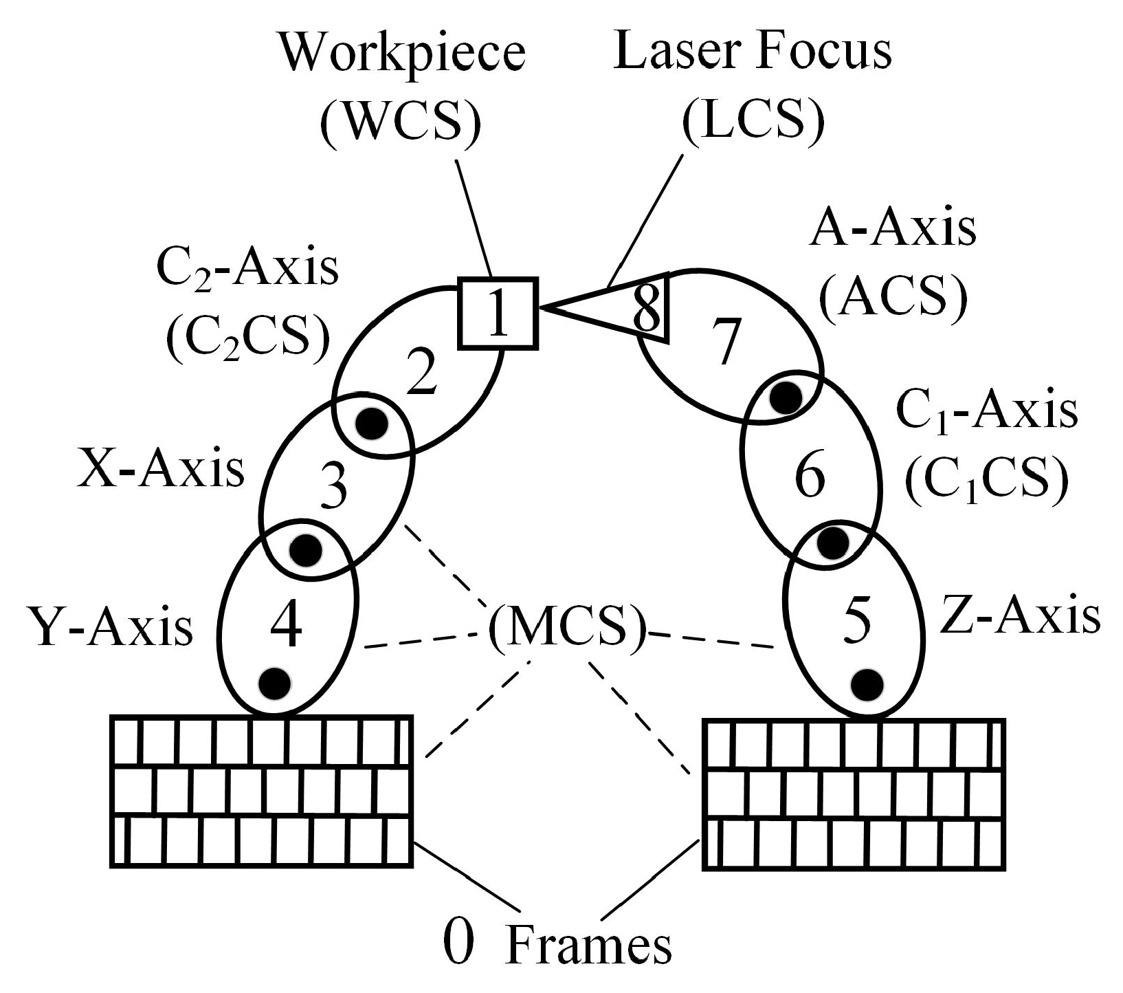
2. Kinematic Model Establishment

To describe the relative motion between the various parts of the machine tools, the kinematic model of the machine tool should be first established. This section establishes a kinematic model of multi-axis LEMT based on HTM, which lays a mathematical foundation for the description of the machine tool motion.

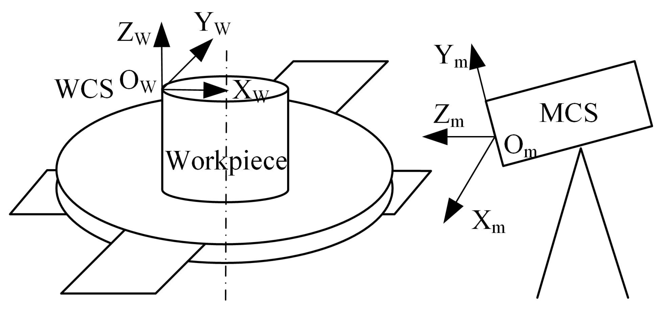
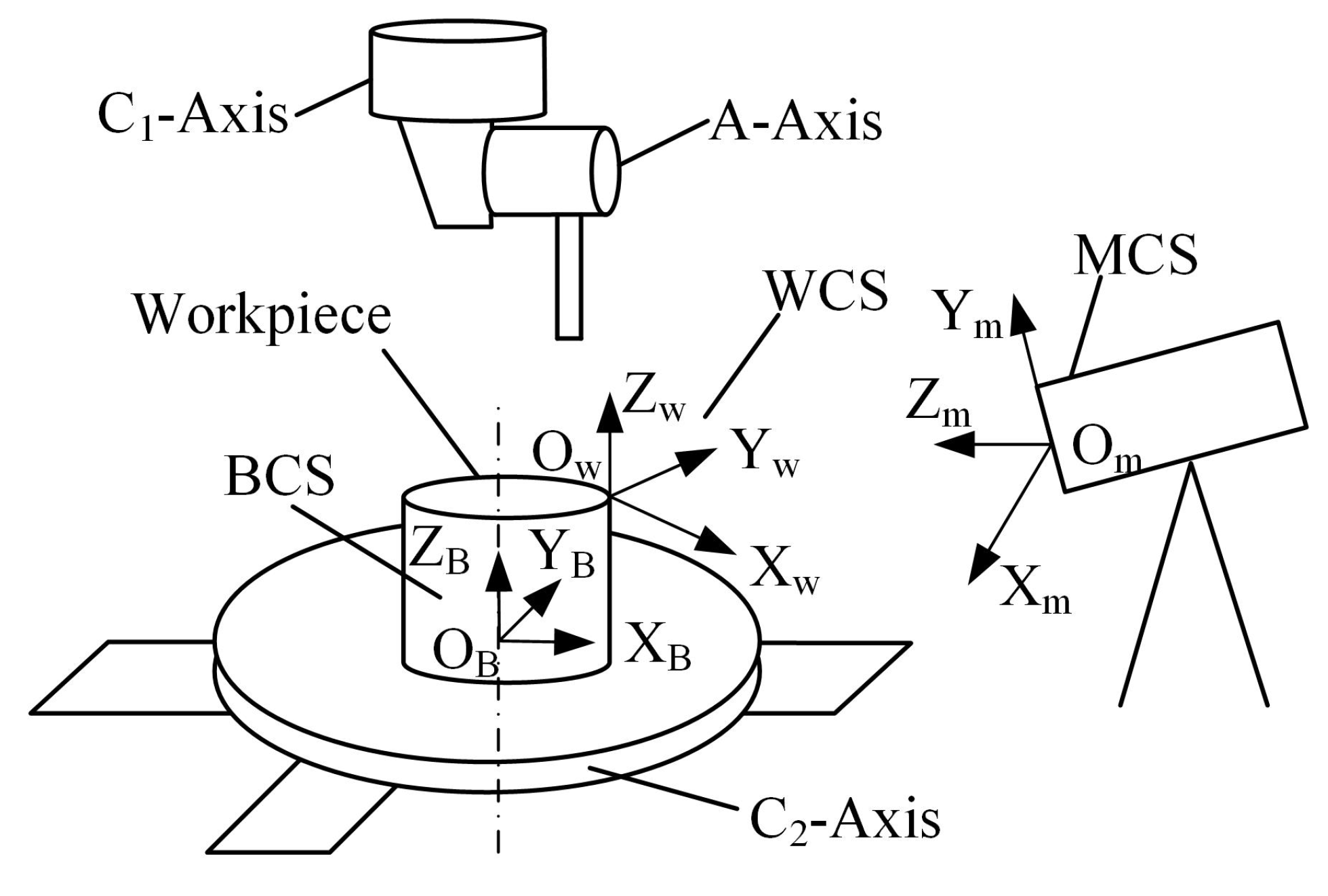
2.1. Coordinate System of Each Component

The structure of the multi-axis LEMT is shown in Figure 1. The main components include three linear axes (X-axis, Y-axis, Z-axis), three rotation axes (A-axis, C 1 -axis, C 2 -axis) and a laser generator installed on the Z-axis slider. The A-axis is defined as a moving part that rotates around the X-axis. The C 1 -axis is defined as the moving part that rotates around the Z-axis and is mounted on the undersurface of the laser generator. The A-axis and C 1 -axis compose a double swing structure, through which the laser beam is directed and focused onto the workpiece. The C 2 -axis is defined as the moving part that rotates around the Z-axis and is mounted on the workbench. The C 2 -axis is used to hold and rotate the workpiece to achieve sub-regional processing when the workpiece is too large to be processed at one time. After the C 2 -axis is fixed at a certain angle, the other five axes (X-axis, Y-axis, Z-axis, A-axis, C 1 -axis) are linked during the processing to perform the complex movement of the laser focus.
The kinematics chain and coordinate systems of the multi-axis LEMT is shown in Figure 2. Four coordinate systems are established to describe the moving components, which are listed as follows: the coordinate system established with the laser spot as the origin is defined as the laser coordinate system (LCS), the coordinate system established with the intersection point of the A-axis rotation centerline and the laser ray as the origin is defined as the A-axis coordinate system (ACS), the coordinate system established with the intersection point of the A-axis rotation centerline and the C 1 -axis rotation centerline as the origin is defined as the C 1 -axis coordinate system (C 1 CS), the coordinate system established with the intersection point of the C 2 -axis rotation centerline and the worktable as the origin is defined as the C 2 -axis coordinate system (C 2 CS). The three positive directions (X/Y/Z) of LCS, ACS, C 1 CS, and C 2 CS are parallel to the positive directions of X-axis, Y-axis, and Z-axis respectively.
The coordinate system formed by rotating the C 2 CS around the Z-axis by the movement angle of C 2 -axis is defined as the basic coordinate system (BCS), the programming coordinate system of the workpiece processing trajectory is defined as the workpiece coordinate system (WCS). During the process of position parameters measurement, the structured light scanner need to be fixed to the proper position. Once the position of the structured light scanner is fixed, a coordinate system will be generated, which is defined as the measurement coordinate system (MCS). The positional relationship between BCS, MCS, and WCS is shown in Figure 3.

2.2. Five-Axis Linkage Transformation

The HTM method was used to establish the kinematic model of multi-axis LEMT. Assuming that each moving component of the machine tool is a rigid body, the motion relationship between them can be represented with a 4 × 4 coordinate transformation matrix.
Figure 4a,b are the front and side view of the double swing structure respectively, several linkage parameters are defined as follows: L t A is the distance between laser beam and the A-axis rotation centerline, R A is the distance from the laser focus to the A-axis rotation centerline, L A C 1 is the staggered distance between the A-axis rotation centerline and the C 1 -axis rotation centerline, R C 1 is the distance from the ACS to C 1 CS. Assume that A is the movement angle of A-axis, the coordinate transformation matrix from LCS to ACS can be represented as:
D L A = 1 0 0 0 0 1 0 L t A 0 0 1 R A 0 0 0 1
The coordinate transformation matrix from ACS to C 1 CS can be represented as:
D A C 1 = 1 0 0 R C 1 0 cos A sin A L A C 1 0 sin A cos A 0 0 0 0 1
Assume that x 0 , y 0 , and z 0 are the position coordinates of the X-axis, Y-axis, and Z-axis respectively, when the origin of the C 1 CS coincides with the center of the C 2 -axis, X , Y , and Z are the displacements of three linear axes, C 1 is the rotation angle of C 1 -axis, the coordinate transformation matrix from C 1 CS to C 2 CS can be represented as:
D C 1 C 2 = cos C 1 sin C 1 0 X + x 0 sin C 1 cos C 1 0 Y + y 0 0 0 1 Z + z 0 0 0 0 1
Assume that the position of laser focus in the C 2 CS is ( p x , p y , p z ), the laser beam direction vector in C 2 CS is ( i , j , k). Because in the LCS, the laser focus is located at the origin of the LCS, which is (0, 0, 0), and the laser beam direction is along the Z+ of the LCS, which is (0, 0, 1), the coordinate transformation from LCS to C 2 CS can be expressed as:
i p x j p y k p z 0 1 = D C 1 C 2 × D A C 1 × D L A × 0 0 0 0 1 0 0 1
After expansion, the five-axis linkage kinematics transformation becomes:
p x = X + x 0 + R C 1 cos C 1 L A C 1 sin C 1 L tA cos A sin C 1 + R A sin A sin C 1 p y = Y + y 0 + R C 1 sin C 1 + L A C 1 cos C 1 + L tA cos A cos C 1 R A sin A cos C 1 p z = Z + z 0 + R A cos A + L tA sin A i = sin A sin C 1 j = sin A cos C 1 k = cos A
The inverse kinematics transformation can be expressed as:
A = arccos ( k ) C 1 = arctan ( i , j ) X = p x x 0 R C 1 cos C 1 + L A C 1 sin C 1 + L tA cos A sin C 1 R A sin A sin C 1 Y = p y y 0 R C 1 sin C 1 L A C 1 cos C 1 L tA cos A cos C 1 + R A sin A cos C 1 Z = p z z 0 R A cos A L t A sin A
The above equations are the mathematical model of five-axis linkage transformation. Through the five-axis linkage transformation, the complex trajectory in WCS can be decomposed into the motion of each axis, and the motion of each axis can also be synthesized into a complex trajectory in WCS conversely. In the five-axis linkage transformation, there are seven unknown parameters: R A , R C 1 , L t A , L A C 1 , x 0 , y 0 and z 0 , which are defined as linkage parameters. These parameters need to be measured one time after the machine tool is assembled.

2.3. Positioning Transformation

After the five-axis coordinate transformation, the coordinate value in LCS is transformed into C 2 CS. C 2 -axis does not participate in the linkage transformation and assume that C 2 is the movement angle of it, the coordinate transformation matrix from C 2 CS to BCS can be expressed as:
D C 2 B = cos C 2 sin C 2 0 0 sin C 2 cos C 2 0 0 0 0 1 0 0 0 0 1
The above-mentioned coordinate transformation is between the various components of the machine tool, and has not included the position of the workpiece. Once the workpiece is fixed, the coordinate transformation from BCS to WCS needs to be established. Assume that x, y, and z represent the translation values from BCS to WCS, α , β and γ represent the rotation values from BCS to WCS. The coordinate transformation matrix from BCS to WCS can be represented as:
D B W = cos β cos γ cos β sin γ sin β x cos α sin γ + sin α sin β cos γ cos α cos γ sin α sin β sin γ sin α cos β y sin α sin γ cos α sin β cos γ sin α cos γ + cos α sin β sin γ cos α cos β z 0 0 0 1
In the positioning transformation, the unknown parameters are x , y , z , α , β and γ , which are defined as positioning parameters. Their values vary with the installation position of each workpiece, and must be measured before each processing.

3. Measurement of Parameters

After the kinematic model of the multi-axis LEMT was established, the parameters need to be measured to ensure the accuracy of the model. There are seven linkage parameters and six positioning parameters in the kinematic model. The measurement is divided into two parts: linkage parameters measurement and positioning parameters measurement. This paper proposed a rapid measure method of linkage parameters, which was performed once after the machine tool was assembled. As for positioning parameters, this paper proposed a direct measurement method based on structured light scanner, which was carried out every time a workpiece was mounted.

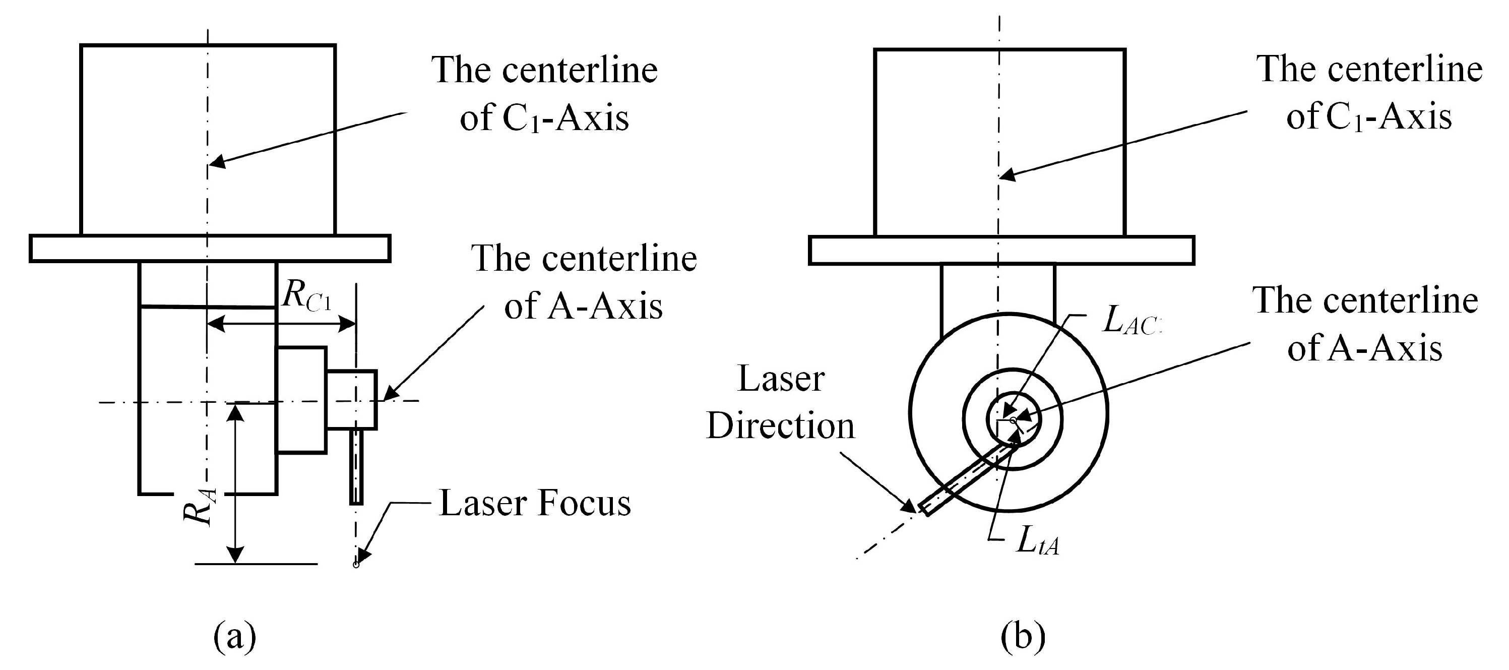
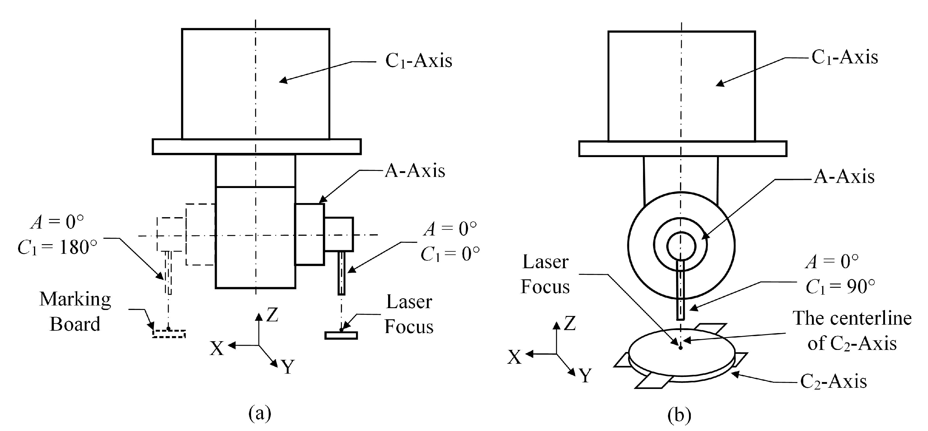
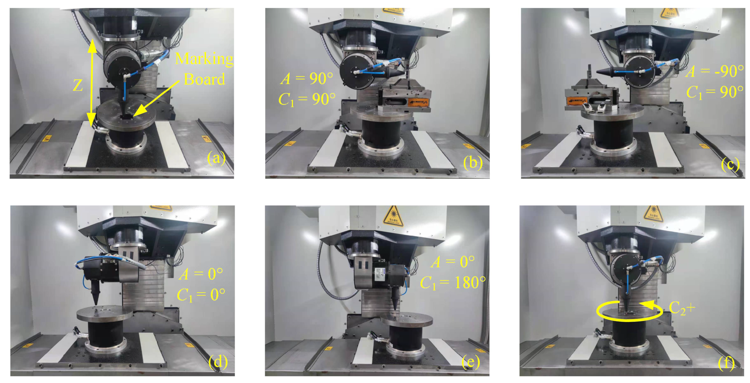
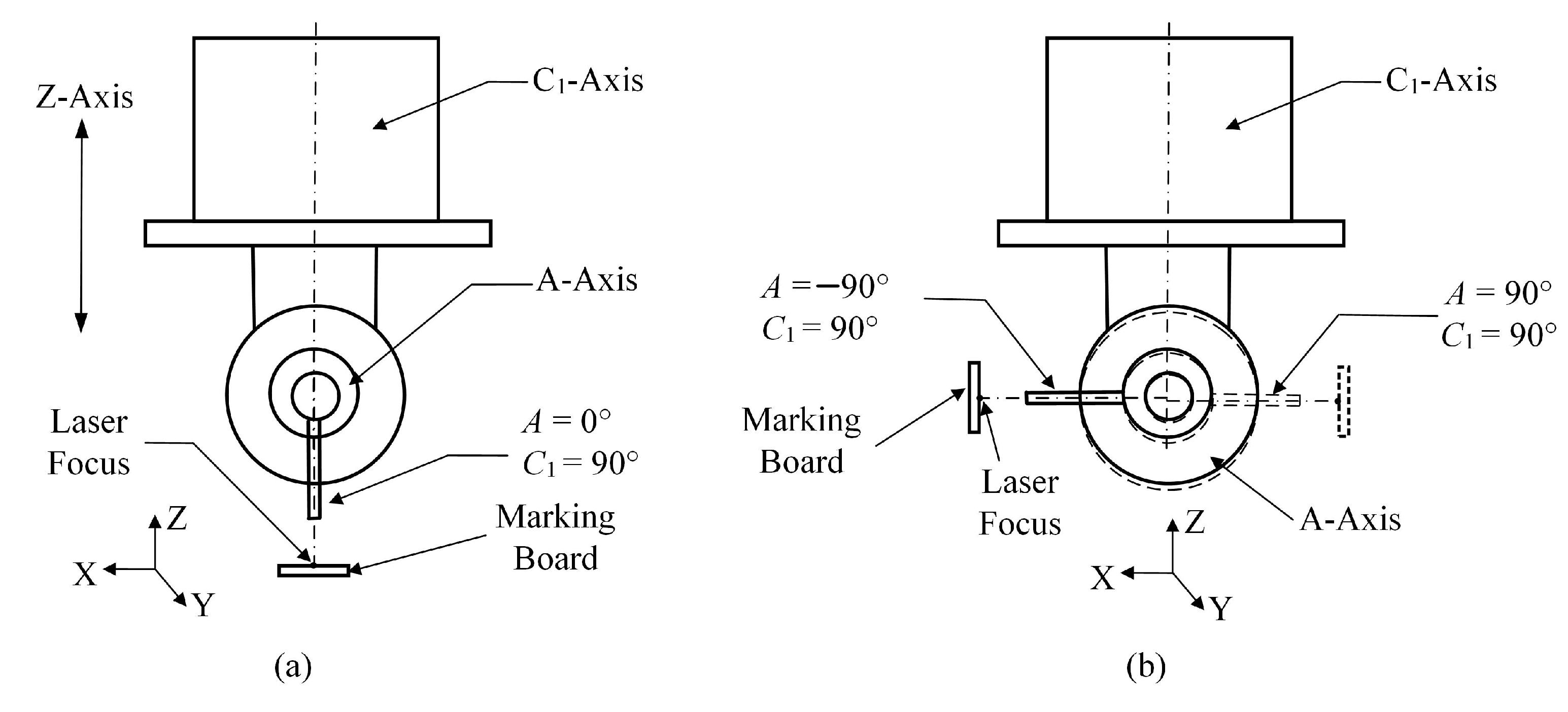
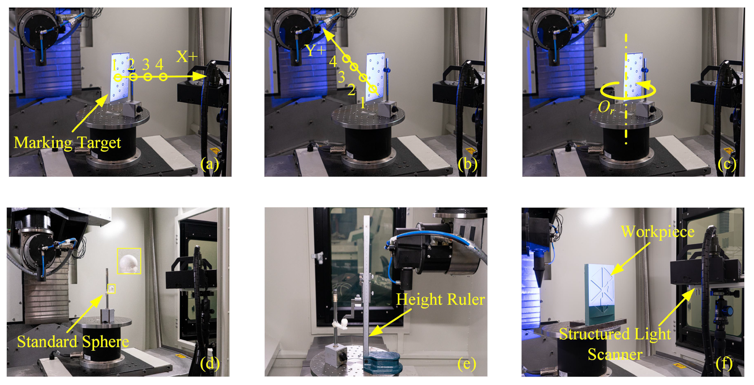
3.1. Measurement of Linkage Parameters

As mentioned above, there are seven unknown linkage parameters in the kinematic model of multi-axis LEMT. This paper proposes a rapid measurement method of linkage parameters taking into account the characteristics of laser processing. This method is implemented by combining the machine tool motion with the laser marking action. The measurement steps of linkage parameters are as follows:
Step 1: Measure the zero point of A-axis and C 1 -axis. Make the laser beam direction parallel to the Z-axis movement direction, and the movement angle of A-axis at this time can be defined as A = 0 . Then make the rotation centerline of A-axis parallel to the X-axis movement direction, define the movement angle of C 1 -axis at this time as C 1 = 0 .
Step 2: Measure the distance from the laser focus to the A-axis rotation centerline ( R A ). As shown in Figure 5a, adjust the A-axis to A = 0 , align the laser exit port with the upper surface of workbench, the displacement of Z-axis at this time is z 1 . Prepare a marking board and place it on the workbench and ensure the upper surface is level. Adjust the Z-axis with a fixed step, move the Y-axis slightly at each position, use the laser focus to draw a line on the marking board. After that, use a microscope to observe the thinnest line or the line width is equal to the diameter of laser focus, the displacement of Z-axis at this time is z 2 . The linkage parameter R A can be calculated as:
R A = z 2 z 1 + d + h
where h is the thickness of the marking board, d is the distance from laser exit port to the rotation centerline of A-axis, which is the known quantity of the machine tool.
Step 3: Measure the distance between laser beam and the A-axis rotation centerline ( L t A ). As shown in Figure 5b, place the marking board perpendicular to the workbench, adjust the C 1 -axis to C 1 = 90 , adjust the A-axis to A = 90 , move the Y-axis slightly, use the laser focus to draw a line on the marking board defined as l 1 . Then, keep the C 1 -axis in C 1 = 90 , adjust A-axis to A = −90 , rotate the C 2 -axis by 180 , move the X-axis to make the laser focus fall on the marking board, move the Y-axis slightly, draw another line defined as l 2 . After that, use a microscope to observe the distance between l 1 and l 2 , which is the linkage parameter L t A .
Step 4: Measure the distance from the ACS to C 1 CS ( R C 1 ) and the staggered distance between the A-axis rotation centerline and the C 1 -axis rotation centerline ( L A C 1 ). As shown in Figure 6a, place the marking board on the workbench, adjust the A-axis to A = 0 , adjust the C 1 -axis to C 1 = 0 , move the Y-axis slightly, use the laser focus to draw a line defined as l 3 , record the position of the X-axis at this time as x 1 , and then move the X-axis slightly, use the laser focus to draw a vertical line defined as l 4 . After that, keep the A-axis in A = 0 , adjust the C 1 -axis to C 1 = 180 , move the X-axis by a large margin to make the laser focus fall on the marking plate again, move the Y-axis slightly, use the laser focus to draw a line defined as l 5 , record the position of the X-axis at this time as x 2 , and then move the X-axis slightly, use the laser focus to draw a vertical line defined as l 6 . After that, use a microscope to observe l 3 to l 6 , the distance between l 3 and l 5 can be defined as e 1 , the distance between l 4 and l 6 can be define as e 2 , the linkage parameter R C 1 can be calculated as:
R C 1 = x 1 x 2 + e 1 / 2
The linkage parameter L A C 1 can be calculated as:
L A C 1 = e 2 / 2 L t A
Step 5: Measure the position coordinates of the X-axis, Y-axis, and Z-axis when the origin of the C 1 CS coincides with the center of the C 2 -axis ( x 0 , y 0 , and z 0 ). As shown in Figure 6b, place the marking board on the workbench, adjust the A-axis to A = 0 , adjust the C 1 -axis to C 1 = 90 , make the laser focus approximately fall on the center of the C 2 -axis, rotate the C 2 -axis, the laser focus will draw a circle on the marking board. And then adjust the position of X-axis and Y-axis continuously until the circle becomes a point, record the position of the X-axis, Y-axis, Z-axis at this time as x 3 , y 3 , z 3 . The linkage parameters x 0 , y 0 , and z 0 can be calculated as:
x 0 = x 3 + L t A + L A C 1 y 0 = y 3 R C 1 z 0 = z 3 R A h
Through the above-mentioned steps, the measurement of seven linkage parameters can be completed. This method makes full use of the characteristics of laser processing and can be conveniently applied to multi-axis LEMT, which does not require the complicated and expensive measuring instruments.

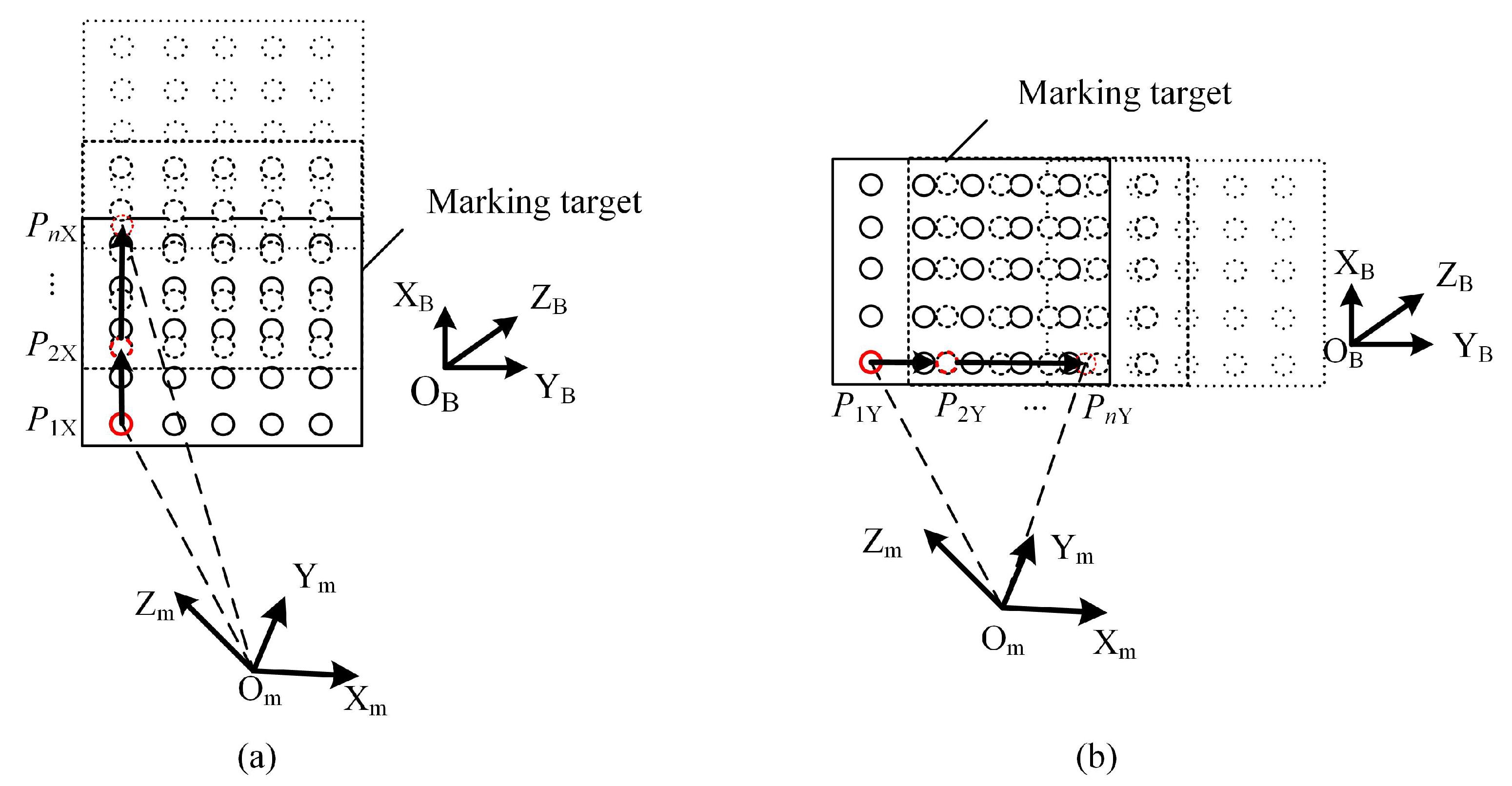
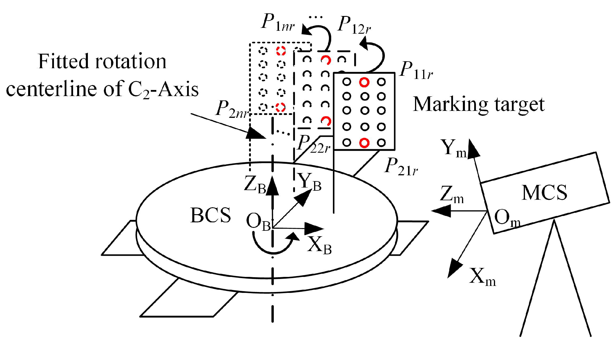
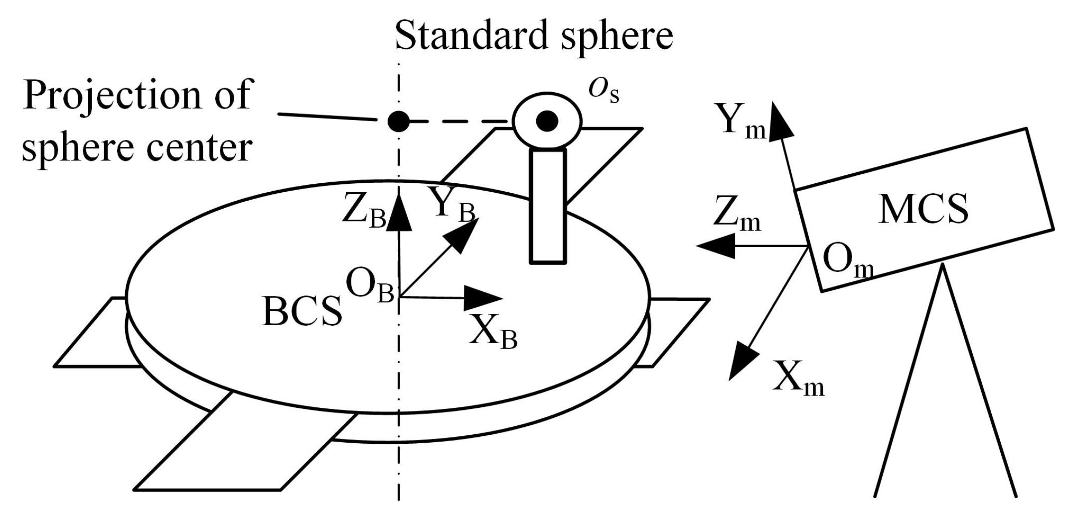
3.2. Measurement of Positioning Parameters

There are six unknown positioning parameters in the kinematic model of multi-axis LEMT. This paper proposes a positioning parameter measurement method by combining the motion of the machine tool with the position of the object measured by structured light scanner. The process of positioning parameter measurement is to obtain the translation values and rotation values from BCS to WCS, which is divided into two parts: measure parameters from BCS to MCS and measure parameters from MCS to WCS. The measurement steps of positioning parameters are as follows:
Step 1: Measure the direction vector of X-axis (in MCS). Fix a marking target on the workbench. Make the X-axis carry the marking target and move several steps in the positive direction, as shown in Figure 7a. During the movement, make the structured light scanner shoot the marking target one time at each position, and record a coordinate (in MCS) of marking target defined as P 1 X , P 2 X P n X respectively. These coordinates can be fitted into a straight line using the least square method, the direction vector of X-axis (in MCS) can be expressed as:
n X = P 1 X P n X P 1 X P n X
Step 2: Measure the direction vector of Y-axis (in MCS), further calculate the rotation matrix from BCS to MCS ( R B M ). Make the Y-axis carry the marking target and move several steps in the positive direction, as shown in Figure 7b. During the movement, make the structured light scanner shoot the marking target one time at each position, and record a coordinate (in MCS) of marking target defined as P 1 Y , P 2 Y P n Y respectively. Similarly, the direction vector of Y-axis (in MCS) can be expressed as:
n Y = P 1 Y P n Y P 1 Y P n Y
According to the orthogonality of the Cartesian coordinate system, the direction vector of Z-axis (in MCS) is: n Z = n X × n Y . Synthesize the above vectors, the rotation matrix from BCS to MCS is: R B M = [ n X n Y n Z ] T .
Step 3: Measure the direction vector of the rotation centerline of C 2 -axis (in MCS). Move the C 2 -axis to a suitable position close to the structured light scanner, and record its position in the CNC system as [ x 0 y 0 z 0 ] T . Make the C 2 -axis carry the marking target and rotate several steps in the positive direction, as shown in Figure 8. During the movement, make the structured light scanner shoot the marking target one time at each position, and record two coordinates (in MCS) of marking target, which are defined as P 11 r , P 21 r , P 12 r , P 22 r P 1 n r , P 2 n r respectively. P 11 r , P 12 r P 1 n r can be fitted into a circle by the least square method, assume that the coordinate of circle center is O 1 . P 21 r , P 22 r P 2 n r can also be fitted into a circle, and the coordinate of circle center is O 2 . Then, the direction vector of the rotation centerline of C 2 -axis can be expressed as:
L = O 2 O 1 O 2 O 1
Step 4: Measure the coordinate of a standard sphere, further calculate the translation parameters from BCS to MCS ( T B M ). Fix a standard sphere on the machine tool turntable, as shown in Figure 9, make the structured light scanner shoot the surface of the standard sphere, and obtain the 3D point cloud data of the surface, use the least square method to calculate the sphere center coordinate, which is defined as o s = [ x s y s z s ] T . The sphere center o s can be projected to L and obtain the projection point o s c . After the action of the rotation matrix R B M , the coordinate of projection point can be expressed as:
o s R = R B M × o s c = [ x s R y s R z s R ] T
Use height ruler measure the distance between o s and the machine tool turntable, the distance is defined as z p . The projection point o s c is on the rotation centerline of the C 2 -axis. So, the coordinate of the projection point in BCS is o p = [ 0 0 z p ] T . Due to the coordinate system conversion relationship is o p = o s R + T B M , the translation parameters from BCS to MCS can be calculated as:
t x = x s R t y = y s R t z = z s R z p
The above calculations are all carried out with the coordinate of C 2 -axis center being [ x 0 y 0 z 0 ] T . When the C 2 -axis center moves to any position in the CNC system, assume that the coordinate is [ x 1 y 1 z 0 ] T , the translation parameters from BCS to MCS can be calculated as:
t x = x 1 x 0 x s R t y = y 1 y 0 y s R t z = z s R z p
The translation matrix from the BCS to MCS can be expressed as: T B M = [ t x t y t z ] T . Synthesize the rotation matrix R B M and the translation matrix T B M , the transformation matrix from BCS to MCS can be calculated as:
D M B = R B M 0 0 1 × 0 T B M 0 1
Step 5: Measure the coordinate transformation matrix from MCS to WCS ( D W M ), further calculate the positioning parameters. Clamp the workpiece to the worktable with the structured light scanner fixed as shown in Figure 10. Make the structured light scanner shoot the workpiece to obtain the 3D point cloud of the workpiece. Perform IRLS-ADF robust registration between the 3D point cloud and the CAM model of the workpiece, the coordinate transformation matrix from MCS to the WCS can be obtained [21]. The coordinate transformation matrix from MCS to WCS can be denoted as D W M , and the transformation matrix from BCS to WCS can be calculated as: D W B = D M B × D W M . Decompose the transformation matrix D B W , the translation values ( x , y , and z) and the rotation values ( α , β and γ ) from BCS to WCS can be calculated.
Through the above-mentioned steps, the measurement of six positioning parameters can be completed. The measurement of the coordinate transformation matrix from BCS to MCS ( D M B ) needs to be done after the structured light scanner is fixed. Remeasurement will not be needed until the position of structured light scanner is changed. Meanwhile, the measurement of the coordinate transformation matrix from MCS to WCS ( D W M ) is carried out every time a workpiece is mounted.

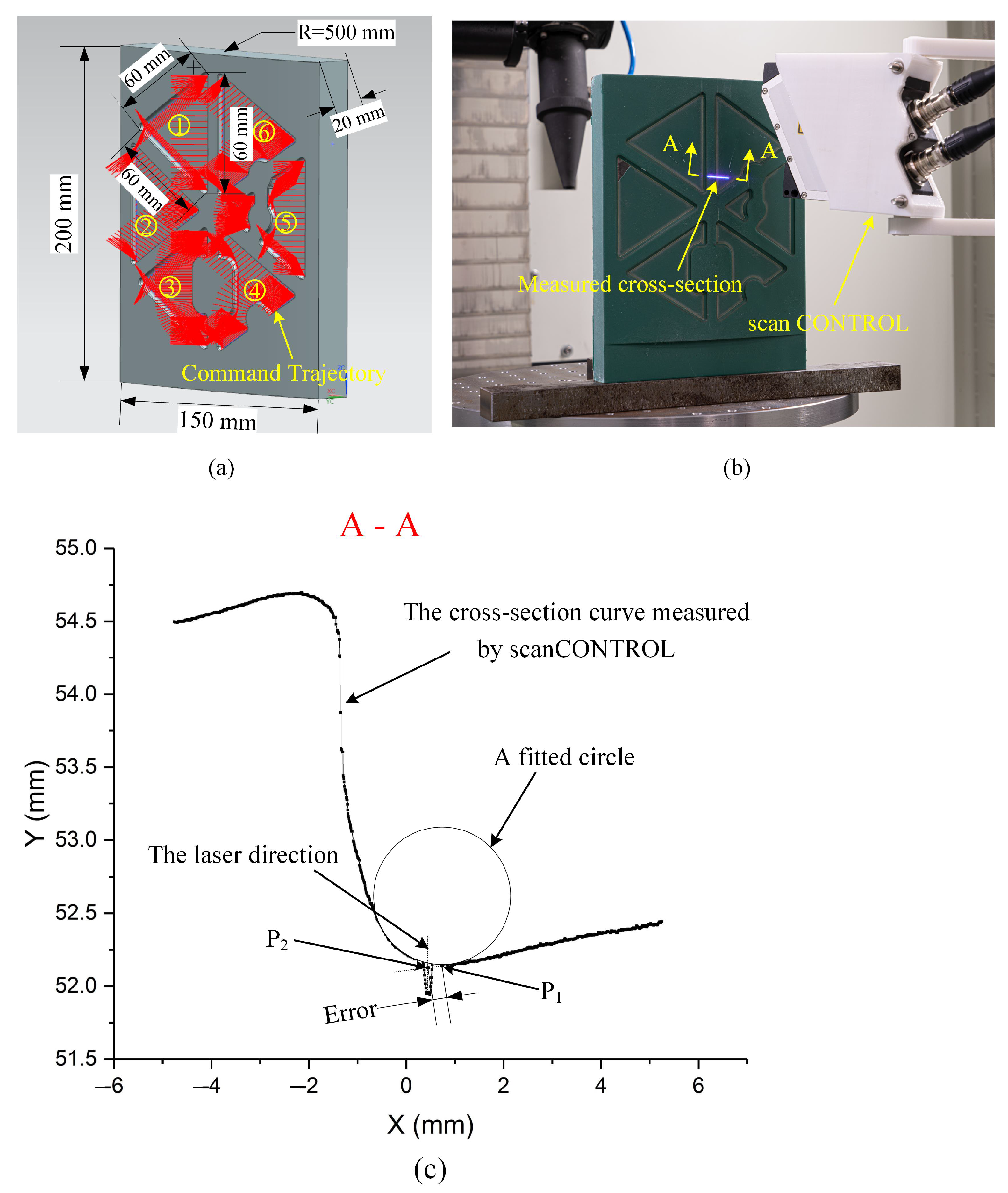
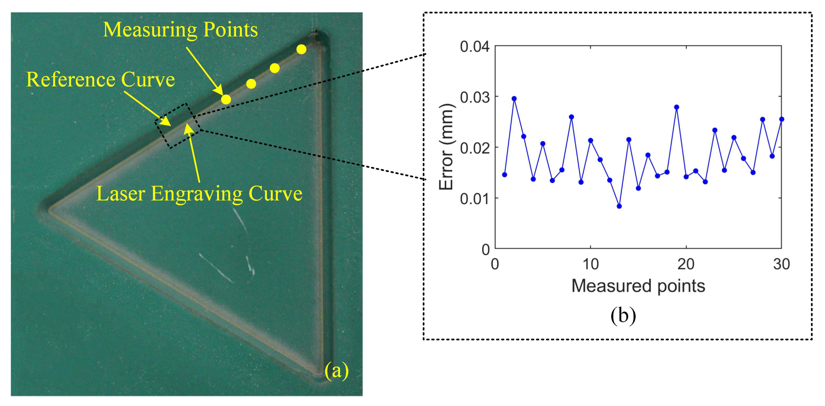
4. Experimental Verification

The feasibility and accuracy of the above measurement methods were experimentally validated using a multi-axis LEMT embedded with an in-house developed CNC system (BH-LaserCNC). The measurement accuracy of linkage parameters and positioning parameters is affected by the motion accuracy of each axis of the machine tool. The definition of motion accuracy is the difference between the actual position reached by the moving part minus the target position (GB/T 17421.2.2016). It is necessary to compensate the positioning accuracy of the six axes before the measurement experiment to ensure its accuracy. The compensated motion accuracy of each axis is shown in Table 1, which was measured by the laser interferometer (XL-80, Renishaw Co., London, UK) . The main technical parameters of XL-80 are shown in Appendix A.
The measurement process of linkage parameters is as shown in Figure 11: Figure 11a shows the measurement process of R A , by continuously adjusting the position of the Z-axis, the thinnest ablation line can be found using microscope (Dino-Lite AM7115, VIDY OPTICS Co., Wuxi, China) The main technical parameters of Dino-Lite AM7115 are shown in Appendix A. After that, R A can be calculated according to Equation (9). Figure 11b,c shows the measurement process of L t A , L t A can be measured by Dino-Lite according to the step 3 in Section 3.1. Figure 11d,e shows the measurement process of R C 1 and L A C 1 , e 1 and e 2 in step 4 can be measured by Dino-Lite similarly, R C 1 and L A C 1 can be calculated according to Equations (10) and (11) respectively. Figure 11f shows the measurement process of x 0 , y 0 , and z 0 , x 3 , y 3 , and z 3 in step 5 can be obtained from the CNC system directly, x 0 , y 0 , and z 0 can be calculated according to Equation (12). Finally, the calculated results of linkage parameters are as shown in Table 2.
The measurement process of positioning parameters is as shown in Figure 12: Figure 12a–c shows the measurement process of the rotation matrix from MCS to BCS ( R B M ), Figure 12d,e shows the measurement process of the translation matrix from MCS to BCS ( T B M ), Figure 12f shows the measurement process of the coordinate transformation matrix from MCS to WCS ( D M W ), the calculated results of linkage parameters are as shown in Table 3.
After the measurement of the above parameters is completed, a spatial curve of test part designed by National Key Research & Development Program of China (2016YFB1102503) is processed to verify the accuracy of the measured values. The contour error of laser engraving is expected to be controlled within 50 μ m. The definition of contour error is as follows: Figure 13a shows the dimension of test part and the command trajectory of laser engraving. The command trajectory is an intersecting curve on a cylinder generated by CAM, which requires multi-axis linkage to achieve. The G code for trajectory coordinates are available on request from the corresponding author. The actual ablation curve formed by laser engraving is defined as laser engraving curve. The distance from the laser engraving curve to the command trajectory is defined as the laser processing contour error.
Figure 13b is the overview of contour error measurement at one point on the curve. The laser scanner (scanCONTROL 29X0, Micro-Epsilon Co., Bavaria, Germany) was applied to measure the cross-section curve (A-A), the main technical parameters of it are shown in Appendix A. A typical cross-section curve (A-A) is shown in Figure 13c, there is a fitted circle at the corner of the curve, P 1 is the intersection of the fitted circle and the cross-section curve, which is a point on the command trajectory. P 2 is the intersection of the tangent line of the fitted circle at P 1 and the direction line of the laser, which is a point on the laser engraving curve. The distance between P 1 and P 2 is defined as the contour error of a certain point on the curve.
A pattern marked ① in the Figure 13a on the test part was taken as an example of the measurement of laser processing contour error, which is shown in Figure 14a. A total of 30 points was taken uniformly on the entire curve, the coordinates of them are shown in Appendix A. The measurement results of the contour errors at every point are shown in the Figure 14b. The maximum error is 29.5 μ m, the average is 15.1 μ m, and the standard deviation is 6.8 μ m. It can be observed from the results that the contour error of laser engraving was controlled within 30 μ m, which is much better than 50 μ m proposed by the key projects mentioned above. Therefore, the parameters measured by proposed methods can effectively ensure the accuracy of the laser processing.

5. Conclusions

In this paper, the kinematic model of the multi-axis LEMT is described and two types of unknown parameters in the model are measured. The methods proposed can be applied to multi-axis laser processing and ensures the processing accuracy. The main conclusions can be summarized as follows:
  • The machine tool kinematic chain was divided into a five-axis linkage part and a positioning part. The HTM method is used to establish a complete kinematic model from the laser focus to the workpiece programming coordinate system. The linkage parameters and positioning parameters are defined as two types of unknown parameters that need to be measured.
  • As for the linkage parameters, a fast measurement method suitable for laser processing is proposed. By combining machine tool motion and laser marking, the measurement of seven linkage parameters can be completed in five steps. This method makes full use of the characteristics of laser processing and does not require the complicated and expensive measuring instruments.
  • Aiming at the positioning parameters, a measurement method based on structured light scanners is proposed. Both translation values and rotation values can be obtained through this method, which can ensure the accuracy of workpiece positioning and thus the accuracy of laser processing.
  • The two types of parameters of a multi-axis LEMT are measured, and the accuracy of the measured parameters is verified by processing a spatial curve. The experimental results show that the average processing contour error can be controlled at 15.1 μ m, which can fulfill the requirements of engineering application.

Author Contributions

Conceptualization, Z.Y., P.S. and J.D.; methodology, Z.Y.; software, J.D.; validation, J.D. and P.S.; formal analysis, Z.Y.; investigation, Z.Y. and Q.L.; resources, Q.L.; data curation, Z.Y. and P.S.; writing—original draft preparation, Z.Y.; writing—review and editing, Z.Y. and Q.L.; supervision, Q.L.; project administration, Q.L.; funding acquisition, Q.L. All authors have read and agreed to the published version of the manuscript.

Funding

This research was funded by National Key Research and Development Program of China (Grant No. 2016YFB1102503).

Institutional Review Board Statement

Not applicable.

Informed Consent Statement

Not applicable.

Data Availability Statement

Not applicable.

Acknowledgments

The first author would like to express his thanks to Hang Z. for offering valuable guidance and support during the writing of this manuscript.

Conflicts of Interest

The authors declare no conflict of interest.

Abbreviations

The following abbreviations are used in this manuscript:
LEMTLaser Engraving Machine Tools
HTMHomogeneous Transformation Matrix
WCSWorkpiece Coordinate System
BCSBasic Coordinate System
D–HDenavit–Hartenberg
CCDCharge Coupled Device
LCSLaser Coordinate System
ACSA-axis Coordinate System
C 1 CSC 1 -axis Coordinate System
C 2 CSC 2 -axis Coordinate System
MCSMeasurement Coordinate System

Appendix A

Table A1. Main Technical parameters of XL-80.
ParameterValueUnit
Measurement Range0–80m
Linear Measurement Accuracy±0.5ppm
Measurement Resolution1nm
Sampling Frequency50mm
Providedby the website: www.renishaw.com (accessed on 1 October 2021).
Table A2. Main Technical parameters of Dino-Lite AM7115.
ParameterValueUnit
Magnification20–220-
Pixel5mp
Image Resolution2592 × 1944dpi
Maximum Frame Rate30fps
Provided by the website: www.vidy.com.cn (accessed on 1 October 2021).
Table A3. Main Technical parameters of scanCONTROL 29X0.
ParameterValueUnit
Z-axis Range8mm
Z-axis Accuracy±0.17%mm
X-axis Range1.3mm
Measurement Points Number (X)1280-
Scanning Frequency2000Hz
Provided by the website: www.micro-epsilon.com.cn (accessed on 1 October 2021).

Appendix B

Table A4. The coordinates of the 30 measured points.
Points
No.
X/(mm)Y/(mm)Z/(mm)Points
No.
X/(mm)Y/(mm)Z/(mm)
181.80322.560188.07216132.46319.484156.434
285.63322.497185.71417130.54419.686154.855
388.98422.421183.65218127.05120.043152.694
492.17522.328181.68719123.23720.405150.337
595.36622.215179.72220119.73920.713148.176
698.71522.073177.66021116.39820.987146.113
7102.06321.915175.59722113.05621.239144.050
8105.41021.733173.53423109.23421.500141.692
9109.23421.500171.17624105.41021.733139.335
10113.05621.239168.81925102.06321.915137.272
11116.39820.987166.7562698.71522.073135.209
12119.73920.713164.6932795.36622.215133.146
13123.23720.405162.5322892.17522.328131.182
14127.05120.043160.1752988.98422.421129.217
15130.54419.686158.0133085.63322.497127.154

References

  1. Nikolidakis, E.; Choreftakis, I.; Antoniadis, A. Experimental Investigation of Stainless Steel SAE304 Laser Engraving Cutting Conditions. Machines 2018, 6, 40. [Google Scholar] [CrossRef] [Green Version]
  2. Song, Z.; Ding, S.; Chen, Z.; Lu, Z.; Wang, Z. High-Efficient Calculation Method for Sensitive PDGEs of Five-Axis Reconfigurable Machine Tool. Machines 2021, 9, 84. [Google Scholar] [CrossRef]
  3. Sieber, I.; Yi, A.; Gengenbach, U. Metrology Data-Based Simulation of Freeform Optics. Appl. Sci. 2018, 8, 2338. [Google Scholar] [CrossRef] [Green Version]
  4. Yu, M.; Zhao, J.; Zhang, L.; Wang, Y. Study on the dynamic characteristics of a virtual-axis hybrid polishing machine tool by flexible multibody dynamics. Proc. Inst. Mech. Eng. Part B J. Eng. Manuf. 2004, 218, 1067–1076. [Google Scholar] [CrossRef]
  5. Sulitka, M.; Šindler, J.; Sušeň, J.; Smolík, J. Application of Krylov Reduction Technique for a Machine Tool Multibody Modelling. Adv. Mech. Eng. 2014, 6, 592628. [Google Scholar] [CrossRef] [Green Version]
  6. Tsai, C.Y.; Lin, P.D. The mathematical models of the basic entities of multi-axis serial orthogonal machine tools using a modified Denavit–Hartenberg notation. Int. J. Adv. Manuf. Technol. 2009, 42, 1016–1024. [Google Scholar] [CrossRef]
  7. Lee, R.S.; Lin, Y.H. Development of universal environment for constructing 5-axis virtual machine tool based on modified D–H notation and OpenGL. Robot. Comput.-Integr. Manuf. 2010, 26, 253–262. [Google Scholar] [CrossRef]
  8. Yang, J.; Altintas, Y. Generalized kinematics of five-axis serial machines with non-singular tool path generation. Int. J. Mach. Tools Manuf. 2013, 75, 119–132. [Google Scholar] [CrossRef]
  9. Xiang, S.; Altintas, Y. Modeling and compensation of volumetric errors for five-axis machine tools. Int. J. Mach. Tools Manuf. 2016, 101, 65–78. [Google Scholar] [CrossRef]
  10. Hsu, Y.Y.; Wang, S.S. A new compensation method for geometry errors of five-axis machine tools. Int. J. Mach. Tools Manuf. 2007, 47, 352–360. [Google Scholar] [CrossRef]
  11. Lee, J.C.; Lee, H.H.; Yang, S.H. Total measurement of geometric errors of a three-axis machine tool by developing a hybrid technique. Int. J. Precis. Eng. Manuf. 2016, 17, 427–432. [Google Scholar] [CrossRef]
  12. Ibaraki, S.; Oyama, C.; Otsubo, H. Construction of an error map of rotary axes on a five-axis machining center by static R-test. Int. J. Mach. Tools Manuf. 2011, 51, 190–200. [Google Scholar] [CrossRef] [Green Version]
  13. Bi, Q.; Huang, N.; Sun, C.; Wang, Y.; Zhu, L.; Ding, H. Identification and compensation of geometric errors of rotary axes on five-axis machine by on-machine measurement. Int. J. Mach. Tools Manuf. 2015, 89, 182–191. [Google Scholar] [CrossRef]
  14. de Araujo, P.R.M.; Lins, R.G. Cloud-based approach for automatic CNC workpiece origin localization based on image analysis. Robot. Comput.-Integr. Manuf. 2021, 68, 102090. [Google Scholar] [CrossRef]
  15. Aguado, S.; Samper, D.; Santolaria, J.; Aguilar, J.J. Identification strategy of error parameter in volumetric error compensation of machine tool based on laser tracker measurements. Int. J. Mach. Tools Manuf. 2012, 53, 160–169. [Google Scholar] [CrossRef]
  16. Guo, S.; Jiang, G.; Zhang, D.; Mei, X. Position-independent geometric error identification and global sensitivity analysis for the rotary axes of five-axis machine tools. Meas. Sci. Technol. 2017, 28, 45006. [Google Scholar] [CrossRef]
  17. Zhu, L.; Luo, H.; Ding, H. Optimal Design of Measurement Point Layout for Workpiece Localization. J. Manuf. Sci. Eng. 2009, 131. [Google Scholar] [CrossRef]
  18. Cheng, F.; Fu, S.; Chen, Z. Surface Texture Measurement on Complex Geometry Using Dual-Scan Positioning Strategy. Appl. Sci. 2020, 10, 8418. [Google Scholar] [CrossRef]
  19. Wang, Y.; Xu, Y.; Zhang, Z.; Gao, F.; Jiang, X. 3D Measurement of Structured Specular Surfaces Using Stereo Direct Phase Measurement Deflectometry. Machines 2021, 9, 170. [Google Scholar] [CrossRef]
  20. Jywe, W.; Hsu, T.H.; Liu, C.H. Non-bar, an optical calibration system for five-axis CNC machine tools. Int. J. Mach. Tools Manuf. 2012, 59, 16–23. [Google Scholar] [CrossRef]
  21. Ding, J.; Liu, Q.; Sun, P. A robust registration algorithm of point clouds based on adaptive distance function for surface inspection. Meas. Sci. Technol. 2019, 30, 75003. [Google Scholar] [CrossRef]
Figure 1. The structure of multi-axis LEMT.
Machines 09 00237 g001
Figure 2. Kinematics chain diagram of multi-axis LEMT.
Machines 09 00237 g002
Figure 3. Positional relationship between BCS, MCS, and WCS.
Machines 09 00237 g003
Figure 4. Schematic diagram of linkage parameters. (a) The front view of the double swing structure. (b) The side view of the double swing structure.
Machines 09 00237 g004
Figure 5. The measurement process of linkage parameters. (a) The measurement process of R A . (b) The measurement process of L t A .
Machines 09 00237 g005
Figure 6. The measurement process of linkage parameters. (a) The measurement process of R C 1 and L A C 1 . (b) The measurement process of x 0 , y 0 , and z 0 .
Machines 09 00237 g006
Figure 7. The measurement process of R B M . (a) Measure the direction vector of X-axis. (b) Measure the direction vector of Y-axis.
Machines 09 00237 g007
Figure 8. The measurement process of C 2 -axis rotation centerline.
Machines 09 00237 g008
Figure 9. The measurement process of a standard sphere.
Machines 09 00237 g009
Figure 10. The measurement process of D W M .
Machines 09 00237 g010
Figure 11. (af) Process of linkage parameters measurement of multi-axis LEMT.
Machines 09 00237 g011
Figure 12. (af) Process of positioning parameters measurement of multi-axis LEMT .
Machines 09 00237 g012
Figure 13. The dimension of the test part and the error measurement process. (a) The dimension of the test part and the command trajectory of laser engraving. (b) Overview of contour error measurement at a certain point. (c) Definition of error of the point P.
Machines 09 00237 g013
Figure 14. Processing results of the test part. (a) The example pattern of measurement. (b) The results of error measurement.
Machines 09 00237 g014
Table 1. Motion accuracy of each axis.
AxisX/( μ m)Y/( μ m)Z/( μ m)A/(arcsec)C 1 /(arcsec)C 2 /(arcsec)
Motion Accuracy2.771.553.551.72.48.3
Table 2. Linkage parameters calculated results.
Linkage Parameters R A /(mm) R C 1 /(mm) L tA /(mm) L AC 1 /(mm) x 0 /(mm) y 0 /(mm) z 0 /(mm)
Calculated Results240.745209.476−0.265−0.145−197.23625.306−528.996
Table 3. Positioning parameters calculated results.
Positioning Parametersx/(mm)y/(mm)z/(mm) α /( ) β /( ) γ /( )
Calculated Results−73.89694.92433.385−0.103−0.034−0.097
Publisher’s Note: MDPI stays neutral with regard to jurisdictional claims in published maps and institutional affiliations.

