Article

Wind Turbine Bearing Temperature Forecasting Using a New Data-Driven Ensemble Approach

1
School of Traffic and Transportation Engineering, Central South University, Changsha 410075, China
2
School of Information and Engineering, Hebei University of Science and Technology, Shijiazhuang 050001, China
*
Author to whom correspondence should be addressed.
Machines 2021, 9(11), 248; https://doi.org/10.3390/machines9110248
Submission received: 26 September 2021 / Revised: 18 October 2021 / Accepted: 22 October 2021 / Published: 24 October 2021
(This article belongs to the Section Turbomachinery)

Abstract

:
The bearing temperature forecasting provide can provide early detection of the gearbox operating status of wind turbines. To achieve high precision and reliable performance in bearing temperature forecasting, a novel hybrid model is proposed in the paper, which is composed of three phases. Firstly, the variational mode decomposition (VMD) method is employed to decompose raw bearing temperature data into several sub-series with different frequencies. Then, the SAE-GMDH method is utilized as the predictor in the subseries. The stacked autoencoder (SAE) is for the low-latitude features of raw data, while the group method of data handling (GMDH) is applied for the sub-series forecasting. Finally, the imperialist competitive algorithm (ICA) optimizes the weights for subseries and combines them to achieve the final forecasting results. By analytical investigation and comparing the final prediction results in all experiments, it can be summarized that (1) the proposed model has achieved excellent prediction outcome by integrating optimization algorithms with predictors; (2) the experiment results proved that the proposed model outperformed other selective models, with higher accuracies in all datasets, including three state-of-the-art models.

1. Introduction

With the increasing clean energy demand and the crisis of fossil energy, wind energy, as a renewable and green type, has attracted more attention than ever and has become important in the world’s energy structure [1]. Wind turbines are mostly located in areas of rich wind energy resources such as wilderness and mountains, where the operating environment is relatively harsh and will have a certain impact on the operation of the wind turbines. Among the different wind turbine components, the gearbox is one of the critical components and the most fault-prone parts in the wind energy conversion system, which directly affects the reliability of wind turbines [2]. The wind turbine gearbox bearing failure is a commonly-appeared fault, which may cause the low efficiency of the wind turbine and rotating stop and even cause the wind turbine structure to be completely scrapped [3]. The bearing temperatures fluctuate with the operation of the wind turbines and the deviations in wear, deform, lubrication, etc., will present dynamic trends of bearing temperature and cause bearing failure when it is worn or damaged by high temperature [4]. If the potential bearing failures are speculated based on collected before the system warning, the active maintenance can be conducted [5,6]. Therefore, the research of the early warning under predictable conditions in gearbox bearing failure is of great significance to the safe operation and reasonable system dispatching in advance for maintenance and repair measures and to improve the reliability and utilization of wind farms [7,8]. Based on the data from the Supervisory Control and Data Acquisition (SCADA) system, the bearing temperature forecasting model can be established to provide an investigation basis for energy supply [9].

1.1. Related Works

With the fast development of data-driven technology, a variety of models are effectively proposed in the research of components fault diagnosis, which include the regression analysis methods and the time series analysis methods [10].
The regression analysis methods aim to find the regression equation between two or more variables with statistical correlation to establish a mathematical model and conduct statistical analysis and prediction [11]. The independence of the data is reflected in the regression analysis that the order of the data can be exchanged. By modeling process, researchers can randomly select data for sequential model training or select a part of data to split the training set and the validation set [12]. Astolfi et al. proposed a regression model based on the artificial neural networks (ANN) for fault diagnosis, in which the input data are power output, external temperature and wind speed, the output data are rotor bearing temperature and vibration amplitude [13]. Zaher et al. also used the neural network structure to handle the multiple input [14]. Integrated with the multi-agent systems (MAS), the proposed techniques can reduce the overall volume of data and effectively improve data processing ability and robustness.
The time series analysis method is a quantitative forecasting method that uses the historical time sequence data of the forecast target, to conduct statistical analysis and construct a mathematical model [15]. The difference between the time series analysis and the regression analysis lies in the assumption of data that the regression analysis assumes that each data point is independent, while time series analysis focuses on the correlation between data for research and take advantage of current data in the absence of other external data [16]. Therefore, time series analysis must search for the corresponding correlation through modeling and use it to predict the future data trend. The time series forecasting models run forward-looking predictions of temperature through effective analysis of data depth information and change trends and then generate real-time early warning [17]. The work of data fitting is then carried out by learning the rules of the training set and the verification set. The direct application of the measured temperature can effectively simplify the workload and avoid the impact of complex data on a real-time early warning.
In recent years, the commonly used time series forecasting models mainly include statistical predictors and artificial intelligence (AI) based models. The models based on artificial intelligence have become popular among researchers by their advanced predictive power [18]. Xiao et al. applied the Least-Square Support Vector Machine (LSSVM) for temperature forecasting of output shaft gearbox in wind turbines [19]. Xiao et al. proposed a stacked sparse autoencoder improved multi-layer perceptron (MLP) in a new framework layer for main bearing temperature prediction of large-scale wind turbines [20]. Abdusamad et al. designed the multiple linear regression (MLR) to analyze the temperature trends with the model residual in wind turbine generators [21]. Chen et al. utilized the radial basis function neural network (RBFNN) with the principal component analysis (PCA) for the predicted output power in early warning [22].
In recent studies, the deep learning models as the advanced neural network have been widely recognized by scholars. Fu et al. established a new wind turbine gearbox bearing temperature analysis framework based on the convolutional neural network (CNN) and the long short-term memory (LSTM) [23]. The prediction results show that the forecasting performance of LSTM is the best among alternative algorithms. Lu et al. proposed a deep belief network (DBN) for the condition monitoring of wind turbine planetary gearbox [24]. The results of the DBN are better than other regression prediction models. Wang et al. utilized the gated recurrent unit (GRU) to construct the predictor in the bearing residual life prediction of wind turbines [25]. The GRU network outperforms other algorithms and achieves the best prediction results. Heydari et al. applied the group method of data handling (GMDH) method to achieve accurate gearbox bearing temperature and lubrication oil temperature [26].
According to the above literature, AI models have been frequently applied for prediction study, the single predictors, however, are not adaptive to all complex nonlinear series data. For further improvement in adaptability and accuracy of forecasting models, researchers have proposed hybrid smart models in the time series field to get higher prediction accuracy, which integrates intelligent algorithms like the data decomposition, the feature extraction and ensemble learning method:
(a) In data preprocessing, the decomposition algorithms are used to eliminate the non-stationarity of the collected data and to make the raw series more predictable with better accuracy. Yu et al. utilized the wavelet packet decomposition (WPD) into the hybrid model to decompose the raw data into several subseries and obtain relatively independent forecasting by the Elman neural network (ENN) [27]. In the paper of Mi et al., the empirical mode decomposition (EMD) is employed with the singular spectrum analysis (SSA) method to decompose the original data into more stationary signals. The experimental results proved that the decomposition model increased the forecasting accuracy of the proposed hybrid model. Wang et al. used the ensemble empirical mode decomposition (EEMD), an upgraded version of EMD, to solve mode-mixing problems and achieve higher prediction accuracy [28]. Gendeel et al. applied the variational mode decomposition (VMD) to handle the variability from the raw power data and the weighted LS-SVM is adopted for deterministic prediction [29].
(b) The feature extraction method aims to alleviate the data redundancy after decomposition, which improves the input for the predictors in the hybrid structure. Khan et al. designed a new wind power forecasting model for large-scale wind turbines, which includes the PCA method to mine the hidden features from raw data and to identify useful information to reduce the dimension [30]. Liang et al. chose the minimal redundancy maximal relevance (MRMR) [31]. The MRMR used the mutual information to obtain the best feature set by the correlation analysis and redundant information among each decomposed IMF and the features. Liu and Li introduced the interpretative structural modeling (ISM) to combine random forest (RF) for the short-term load forecasting of wind power [32]. Jaseena and Kovoor applied the stacked autoencoder (SAE) to extract more meaningful and brief features from the original dataset for better improvement in the optimal stacked LSTM network of the hybrid model [33].
(c) Ensemble learning can generate feature extraction results and integrate the multiple predictors to have better performance in hybrid models. Nie et al. used the multi-objective grey wolf algorithm (MOGWO) method to integrate three neural network predictors. Experimental results presented that ensemble learning worked better than single predictive models in power forecasting [34]. Zhang et al. proposed the tabu search (TS) into a hybrid model for the integration of predictors and greatly raised the load forecasting accuracy [35]. Wen designed the ant colony optimization (ACO) algorithm with extreme learning machine (ELM), in which the ACO improve the ELM by optimizing network connection weights in the training process to avoid the local minima and obtain accurate forecasting results [36]. In the research of Li et al., particle-swarm optimization (PSO) is employed in an ensemble mechanism to combine the prediction results from short-term and long-term predictors [37].
According to the literature survey, the integrated algorithms of the abovementioned models effectively reduced the errors indexes of the hybrid models. The following points can be elucidated: (1) the decomposition algorithms can greatly remove the non-stationarity in the raw data and increase the recognition ability of the predictors as data preprocessing; (2) the feature extract methods collect the meaningful information from decomposed sub-series and improve the characteristics of the input features to the predictors; (3) the ensemble learning methods can study the mutual influence and independent relationship between data series for weight coefficient optimization with minimal error. Because of the above conclusions, these useful methods can be specifically used in the new framework of bearing temperature prediction.

1.2. The Novelty of This Paper

Inspired by the abovementioned algorithms, a new hybrid ensemble prediction approach VMD-SAE-GMDH-ICA is firstly developed for wind turbine bearing temperature prediction. The novelty of this study is concluded in detail as:
(a) In the study, a novel gearbox bearing temperature prediction model is proposed to accomplish early status prediction of wind turbines. It can effectively achieve valuable information from the SCADA data without additional sensors or measuring systems to analyze the fluctuation tendency for potential failures. Based on the collected signals from the normal working condition, the proposed model can offer practical detection and accurate prediction for early warning and the wind turbine monitoring system can also avoid the difficulty of collecting the information from faulty conditions.
(b) Previous wind turbine temperature research barely studied the VMD decomposition model for the predictors in hybrid structures. VMD can avoid the shortcoming of mode-mixing of the traditional EMD with better decomposition ability and noise resistance and effectively reduce the non-stationary original temperature data in the study.
(c) The SAE-GMDH is used as the predictor to conduct the independent prediction in each subseries decomposed by VMD. SAE is used to extract the primary features with detailed information of the raw temperature series. Compared with a single predictor, the SAE-GMDH has a significant increase in accuracy.
(d) The ICA is first applied in bearing temperature prediction to combine the results by optimizing the weight coefficients. The ICA has been proven to be effective in the optimization process, in which this method has higher convergence accuracy speed and better global optimization than the traditional biological heuristic algorithms PSO and genetic algorithm (GA) [38,39,40]. Therefore, the internal correlation of the bearing temperature series of gearbox can be further investigated, which improves the time-series prediction performance of the wind turbine monitoring system.

2. The Proposed Methodology

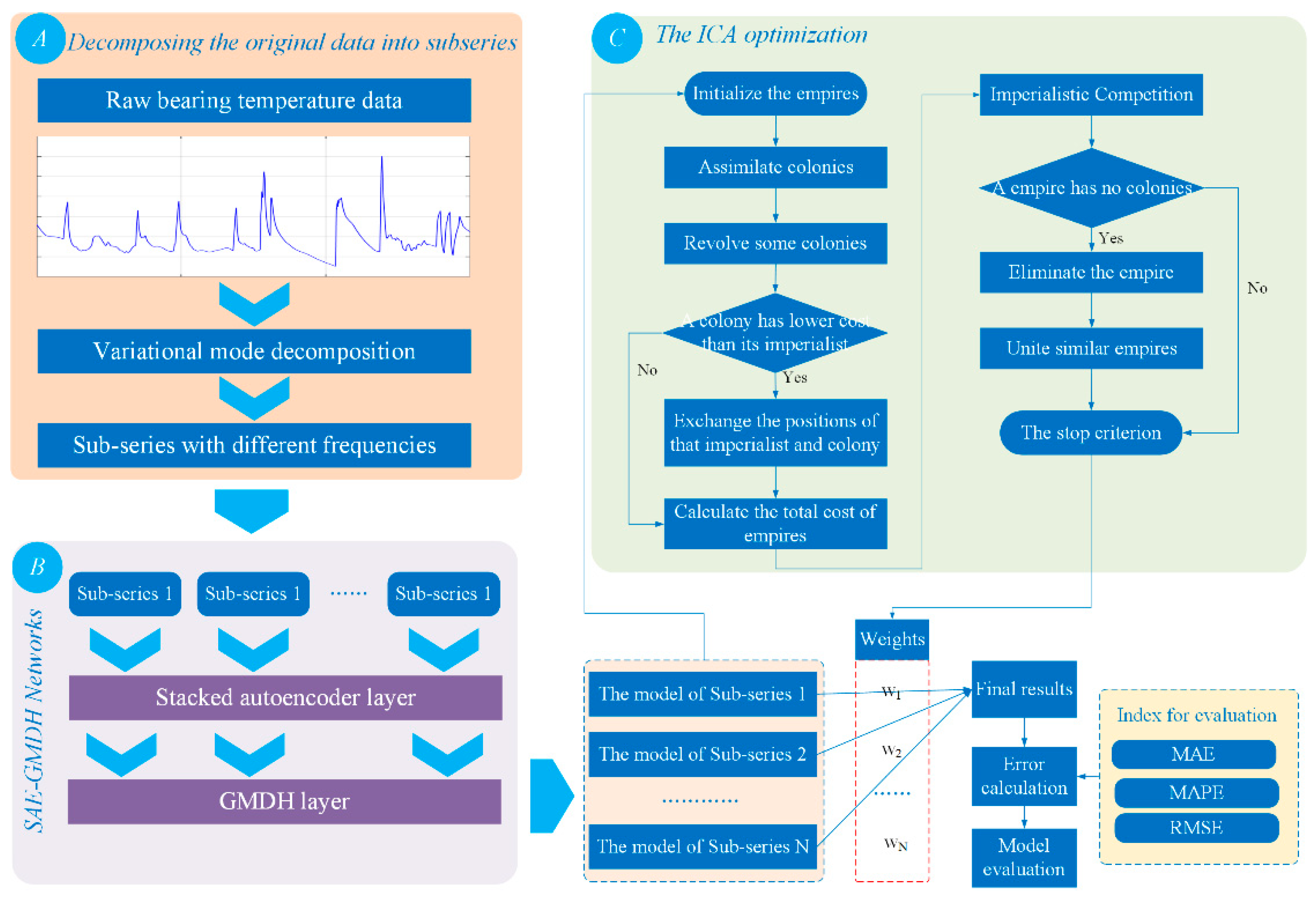
2.1. Topology Framework of the Applied Bearing Temperature Model

The topology modeling process of the applied hybrid model is presented in Figure 1, which includes the decomposition methods, the feature extraction methods and the ensemble learning methods. The specific process can be described as follows:
Part A: The raw bearing temperature data will be preprocessed into training sets, validation sets and testing sets. The VMD is firstly used to preprocess the raw data by decomposing bearing temperature data into independent sub-series, which are then used to train SAE-GMDH. The validation sets are for the training of ICA and test sets are for the testing of the whole model.
Part B: The SAE-GMDH is used to conduct predictions for the sub-series. Based on the principle of unsupervised learning, SAE can obtain plenty of characteristic information from the extraction process of sub-series, which is transmitted into the GMDH network in the next step.
Part C: The ICA method can integrate all the sub-series in the hybrid mechanism. The ensemble learning process is enforced by matching the suitable weight coefficient to the sub-series for the best ensemble results. The ICA method analyzes the features of sub-series results and calculates the weights in eight sub-series to obtain the satisfying final results in all cases.

2.2. Variational Mode Decomposition

The variational mode decomposition (VMD) was first designed by Dragomiretskiy and Zosso [41], which decomposes the basic data into N band-limited intrinsic mode functions. Different from EMD-based methods, VMD can overcome the issues of the end effects and modal component aliasing and decrease the non-stationarity of complex raw data, aiming at comparatively stable sub-sequences containing multiple different frequency scales [42]. In the VMD algorithm, the raw data f(t) is separated into N parts to ensure that the decomposed result is a modal component on a limited distribution with a specific frequency. Moreover, the sum of the approximated distribution should be the smallest and equal to the raw data and the constraint condition is the same for all modes. Then, the related constraint variational equation can be given as follows [43]:
{ min g n , w n { n = 1 N t [ ( δ ( t ) + j π t ) g n ( t ) ] e j w n t 2 2 } s . t . n = 1 N g n = f ( t ) }
where t represents the time script; g n and w n are the set of sub-signals and the specific frequencies; N counts for the number of sub-series; δ ( t ) means Dirac distribution; and is the convolution operator. The penalty term and Lagrangian multipliers are introduced to transform the optimization into unconstrained condition, which is expressed as [44]:
L ( g n , w n , λ ) = β n = 1 N t [ ( δ ( t ) + j π t ) g n ( t ) ] e j w n t 2 2 + f ( t ) n g n ( t ) 2 2 + λ ( t ) , f ( t ) n g n ( t )
where β is a secondary penalty factor and its function is to decrease the disturbance from Gaussian noise and λ is the Lagrange multiplication operator. The alternate direction method of multipliers obtains each modal component and center frequency. The saddle point of the augmented Lagrangian will also be searched. Therefore, the corresponding unconstrained situation can be solved. The g n , w n and λ after alternate optimization iteration can be updated as [45]
g ^ n m + 1 ( w ) = f ^ ( w ) i n g ^ i ( w ) + λ ^ ( w ) 2 1 + 2 β ( w w n ) 2
w ^ n m + 1 = 0 w | g ^ n m + 1 ( w ) | 2 d w 0 | g ^ n m + 1 ( w ) | 2 d w
λ ^ m + 1 ( w ) = λ ^ m ( w ) + γ ( f ^ ( w ) n g ^ n m + 1 ( w ) )
where m is the number of iterations, γ is the noise tolerance to meet the fidelity requirement of signal decomposition; f ^ ( w ) , g ^ i ( w ) , λ ^ ( w ) and g ^ n m + 1 ( w ) are Fourier transforms of f ( t ) , g i ( t ) , λ ( t ) and g n m + 1 ( t ) .

2.3. Stacked Autoencoder

An autoencoder is a feedforward neural network of unsupervised learning algorithms. The model can obtain a good representation of data dimension reduction [46]. The AE can be stacked to construct a deep predictor, which is called stacked autoencoder (SAE). It is composed of multi-layer AEs and output from the previous layer of AEs will be used as input of the next layer to calculate the errors by subtracting the reconstructed data from the input. The specific training process of feature extraction can be summarized as follows [47]:
Step 1: Using the original data as input, the parameters of the first hidden layer will be trained and applied to obtain the output by calculation.
Step 2: Using the result from the first hidden layer as the input of the second hidden layer, the same calculation will be run to get the output of the second layer.
Step 3: Repeat step 2 to initialize the parameters of the deep network through layer-by-layer unsupervised learning pre-training for all automatic encoders.
Step 4: Find the parameter value close to the minimum of the above loss function and transmit it as the final optimal parameter value into the predictor. Then, the supervised learning process will start to train the predictors.

2.4. Group Method of Data Handling

The group method of data handling (GMDH) is a heuristic self-organizing algorithm to obtain the optimal complex model [48]. The generic connection between input and output in the GMDH follows the principle of Kolmogorov–Gabor polynomial approximation as below [48]:
y ^ = A + i = 1 n B i x i + i = 1 n j = 1 m B i j x i x j + i = 1 n j = 1 n k = 1 n D i j k x i x j x k +
where { x 1 , x 2 , x 3 , x n } are the input variables of the network, { A , B , C , } are the weights and the y ^ represents the output of the system.
The K-G polynomial construction of the nonlinear system is realized by adding input variables in each layer of the neural network. To obtain the regression polynomial, the following equation will be used for each pair of input and the output of the training set [49]:
y ^ n = a 0 + a 1 x n i + a 2 x n j + a 3 x n i 2 + a 4 x n j 2 + a 5 x n i x n j
where xni and xnj represent the input variables of the network. The calculation of the weights a 1 ,   a 2 ,   a 3 ,   a 4 ,   a 5 is obtained from the minimum value of the mean square error (MSE) between the actual values and the output values [50]:
MSE = i = 1 n ( y ^ i y i ) 2 / n

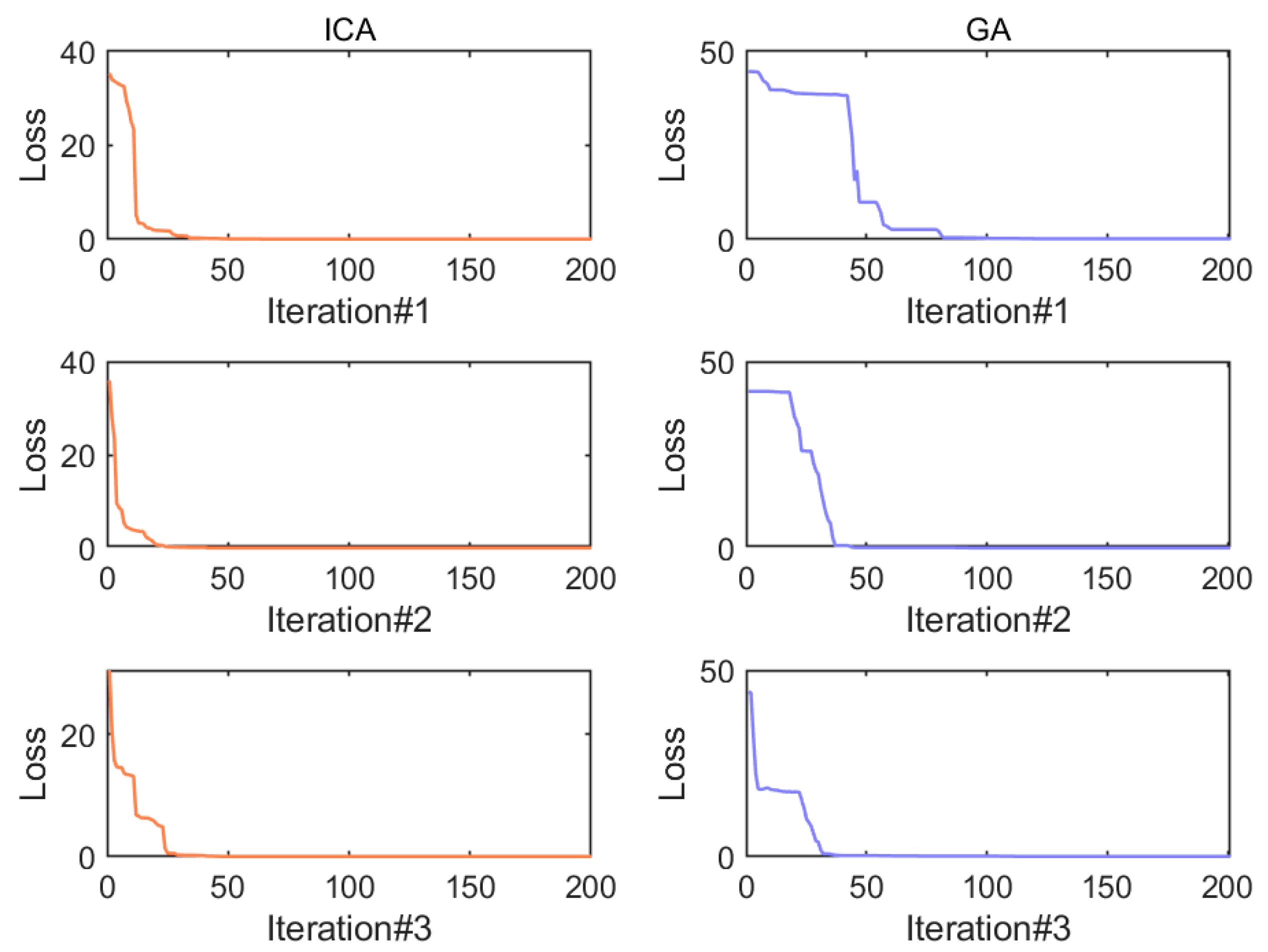
2.5. Imperialist Competitive Algorithm

The Imperialist Competitive Algorithm (ICA) was designed by Atashpaz-Gargari and Lucas in 2007, which is an evolutionary algorithm with the principle of imperialist colonial competition mechanism [51]. The ICA is one of the socially inspired random optimization methods and has higher accuracy and better global convergence than the common PSO and GA algorithms to find the global highest or lowest value [52]. The individuals of ICA are called countries, which are divided into two sections parts: the colony and imperialist. Similar to the chromosomes in the genetic algorithm (GA), the countries of the two parts create an empire. To solve a multivariate optimization problem, a country in ICA consists of 1 × N array which is described as following formula [17]:
c o u n t r y = [ v 1 , v 2 , v 3 , v N ]
where vi is the optimized variable. The variables are regarded as the social and political attributes of the country. The cost of each country is determined by a function f composed of variables as follows:
cost = f ( c o u n t r y ) = f ( [ v 1 , v 2 , v 3 , v N ] )
The process of ICA optimization begins with initializing of countries of size Ncountry and the imperialists Nimperialist. Other countries are used as the colonies Ncolony, which are divided by initial strength to form the original empires. Therefore, the normalized imperialist cost for colonization of the counties is defined in the following formula:
C n = max i { c i }
where cn represents the cost of the n-th imperialist and Cn stands for normalized cost of n-th imperialist. The max i { c i } is the imperialist of the highest cost. The normalized power from the imperialist (vn) is:
v n = | C n i = 1 N i m p e r i a l i s t C i |
The distribution of the original colonies depended on the power of the imperial group to which they belonged. Thus, the number of the colonies owned by the N-th empires:
N . C n = round { P n . N c o l o n y }
where round means a function for the round numbers. N.Cn stands for colonies owned by the nth empire and Ncolony represents the initial colonies [53].
The next assimilation is the approaching of the colony to the empire by the language and culture. After the assimilation is completed, the cost functions of the empire and the colony will be compared. If the cost function from an empire is higher than a colonized country, the empire will become a colony and the colony will become an empire. Figure 2 shows the trajectory of colonies to the appropriate imperialist, in which the colony goes through x units towards the imperialist, is described as:
x U ( 0 , θ × d )
where d represents the interval from the colony towards the imperialist and θ represents a random number between 1 and 2 [54].
The overall strength of an imperialist can be described as
T . C n = f ( i m p n ) + β × i = 1 N . C n f ( c o l i ) N . C i n
where the impn is the imperialist country of the nth empire; T.Cn is the entire cost of the n-th empire; 0 < β < 1 the size of β determines the degree of influence of the colonial country on the entire empire. The weakest colony will be chosen among the weakest empires as the object of empire competition. The competition between empires makes powerful empires stronger by taking the colonies from other empires. Meanwhile, the colonies of weak empires keep decreasing. An empire will be destroyed when it has lost all the colonies. With the demise of the empires, only one empire is left and the ICA algorithm stops running [55].
In this paper, the mean square error (MSE) is applied as the objective function,
MSE = ( t = 1 N [ r ( t ) r ^ ( t ) ] 2 ) / N
where r ( t ) is the original data, r ^ ( t ) is the predictive result and N represents the samples in the raw datasets. Corresponding to the n decomposed subsequences from VMD, the state matrix W can be constructed as the weight matrix,
w = [ w 1 , w 2 w n ]
where w 1 ,   w 2 w n is the corresponding weight and n is the number of the decomposed subsequences after the VMD. The product of each subserie forecasting result matrix and weight matrix will be compared to original data by the optimization algorithm to get the satisfying results in the objective function. The iteration ends up with a satisfying condition. The test set is inputted into the trained framework for the results. The ICA method determines the optimal weight according to the data characteristics of the test set.

3. Case Study

3.1. Description of Bearing Temperature Data

Three SCADA datasets of 1500 samples, with the 10 min interval of wind turbine bearing temperatures, were applied to test the prediction performance of the designed hybrid models in the paper. The SCADA system in the wind turbine can accomplish the functions such as data acquisition, components monitoring and system control, etc. [56,57]. The datasets #1, #2 and #3 were collected from different wind turbine gearbox bearings without data filtering by production requirements to analyze the forecasting performance. The original data are continuously sampled at 10 min intervals under the continuous working state of the wind turbine with the operating power of 2 MW. Table 1 illustrates the statistical results of the temperature time series. The data fluctuation in the time series is shown in Figure 3. The first 900 samples are selected as a training set. The 901st–1200th samples are regarded as the validation set. The last 300 samples are used as the testing set. The training set is used for the data samples for model fitting. The validation set can be used to adjust the optimization algorithm parameters of the model and to make a preliminary assessment. It is usually applied to verify the generalization ability such as the accuracy rate of the proposed model during iterative training of the model to decide whether to stop training. The test set is used to evaluate the predictive ability of the final model framework. The prediction results, which are the outcome from the proposed hybrid model, are applied to compare with the testing set to test the accuracy. All experiments in the study will be established and tested on the Matlab2020a platform, using Windows 10 operating system of a personal computer.

3.2. The Evaluation Indexes

The evaluation indexes will comprehensively show the ability of the proposed model. In this study, three evaluation indexes, which include the mean absolute error (MAE), the root mean square error (RMSE) and the mean absolute percentage error (MAPE), are applied to evaluate the prediction accuracy. To better compare the pros and cons of different models, the promoting percentages of the RMSE, MAPE and MAE are also utilized. The equations of indexes are described as
{ MAE = ( t = 1 N | r ( t ) r ^ ( t ) | ) / N MAPE = ( t = 1 n | ( r ( t ) r ^ ( t ) ) / r ( t ) | ) / N RMSE = ( t = 1 n [ r ( t ) r ^ ( t ) ] 2 ) / N
{ P MAE = ( MAE 1 MAE 2 ) / MAE 1 P MAPE = ( MAPE 1 MAPE 2 ) / MAPE 1 P RMSE = ( RMSE 1 RMSE 2 ) / RMSE 1
where r ( t ) is the measured denotes the raw bearing temperature data, r ^ ( t ) is the predicted bearing temperature data and N represents the samples in the raw datasets. From the above formulas, it can be seen that the smaller values of the evaluation indexes mean smaller deviations between the real data and the prediction results and better prediction accuracy of the models. The bigger values of promoting percentages represent a greater improvement of the prediction accuracy between different models.

3.3. Comparative Analysis with Experiments

3.3.1. Comparison and Analysis of Individual Predictors

To analyze the predictive performance of individual group method of data handling (GMDH) in depth, it will be compared with some traditional predictors and deep learning predictors including the long short-term memory (LSTM), gated recurrent unit (GRU), Elman neural network (ENN), deep belief network (DBN), multi-layer perceptron (MLP), extreme learning machine (ELM), general regression neural network (GRNN), GMDH and radial basis function neural network (RBFNN) for specific research. According to the information Table 2, it is concluded that:
(a) The forecasting accuracy of the GRNN, ELM, MLP and ELM methods are lower than deep learning predictors in all cases, which may be affected by the high volatility and nonlinear features of the raw data series. The deep networks could increase the power to deal with the special features of the raw temperature data by iterative calculation to achieve better robustness than the shallow neural networks.
(b) In the classic deep learning networks, the prediction accuracy of GRU and LSTM in the results is better than others. The possible cause may be that the gated framework can improve the calculation and extract more information of series to construct the framework by multiple hidden layers, which help the GRU and LSTM for better learning capacity of the deep information acquisition from the bearing temperature series.
(c) In comparison with other deep learning models, the GMDH method receives the best prediction output in all datasets. It shows the GMDH has high forecasting ability and application potential. The possible reason is that the GMDH has the self-organizing mechanism of the multi-layer neural network, which improves their ability to automatically retain useful variables and select the suitable parameters to avoid information redundancy and local minimum.

3.3.2. Comparison and Analysis of Different Hybrid Models

To comprehensively verify the predictive ability of the proposed model, the proposed hybrid VMD-SAE-GMDH-ICA model will be analyzed with several selective models by the following experiments:
(a) To evaluate the power in the data preprocess aspect of the decomposition algorithms in bearing temperature prediction, the results of VMD are listed with that of the EEMD and EMD methods by the promoting percentages.
(b) To test the significant improvement by SAE and ICA for the total accuracies, the hybrid VMD-SAE-GMDH and VMD-SAE-GMDH-ICA models are compared with other models in Table 3 and Table 4.
(c) The experiments also compare the ICA with GA (genetic algorithm) to show the research potential of ICA by ensemble learning. Figure 4 displays the changing trend of loss values through the iterations of ICA and GA.
From Table 3, Table 4, Table 5 and Table 6 and Figure 4, it can be summarized that:
(1) Combining the decomposition algorithms in the hybrid structures, the models could achieve better results with higher accuracy than the models without decomposition methods in all datasets. The probable inference may be that decomposition algorithms could decrease the fluctuation character by decomposing the raw data time series into multiple sub-series. From Table 4, the experiment results can also clearly reflect that the decomposition method can effectively improve the prediction accuracy of the predictor GMDH. All the hybrid models with decomposition methods have improved accuracy on the basis of GMDH. Compared with EEMD and EMD, the VMD can achieve better temperature series preprocessing results. With extra noise of the EMD and EEMD function may bring the residual noise when decomposing the original temperature series. VMD presents excellent noise resistance and better decomposing performance, which enable the extracted feature information of time series to be detailed and accurate for better results.
(2) SAE and ICA are used to further increase the power of VMD-GMDH. SAE is applied to obtain useful information from the sub-series and present a better feature description than the original data to GMDH. The ICA ensemble method is applied to analyze and select features of the subseries for weight coefficient and to give the optimal output. In contrast to GA, ICA could get improved calculation results. Different from the traditional biological heuristic algorithm, ICA, as a social heuristic algorithm, has better convergence and faster calculation speed. The results prove that the ICA algorithm has a better application value in optimization capacity than the conventional ensemble methods, which enables the ICA algorithm to get great value in ensemble learning and further increase the predictive precision.

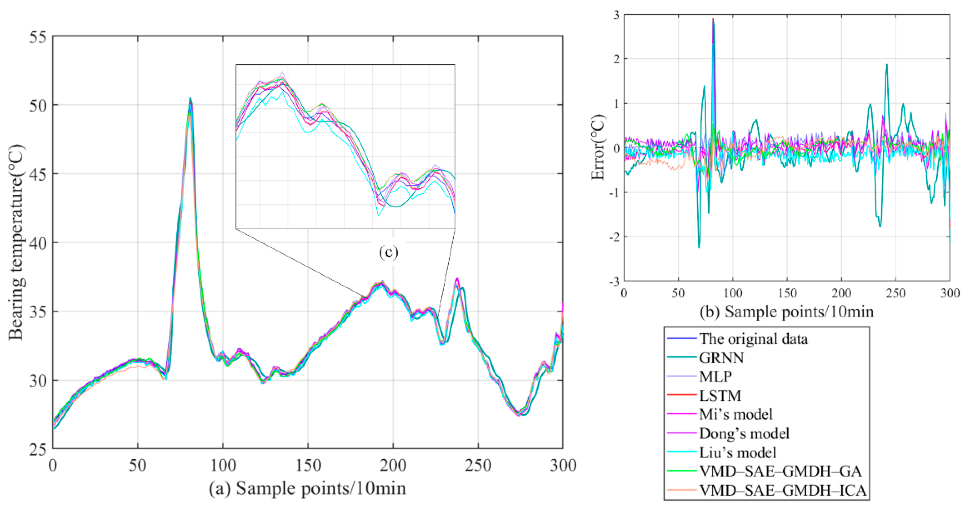
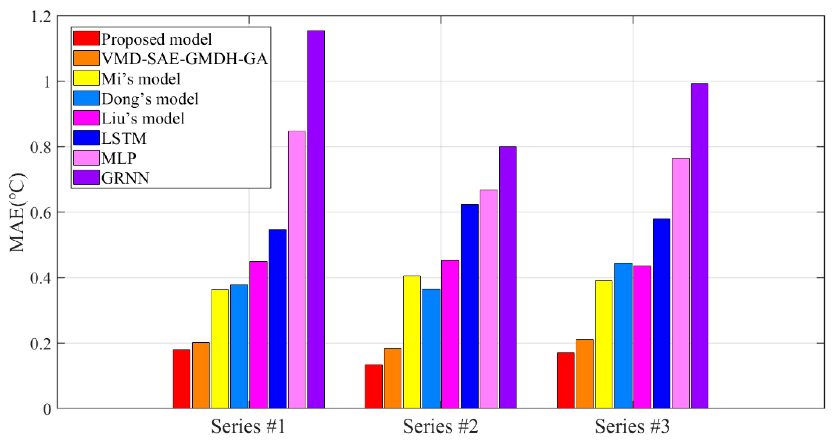
3.3.3. Comparison and Analysis of Existing Models

To prove the availability and innovation of the designed VMD-SAE-GMDH-ICA model, it is essential to essential the analysis with several existing advanced models in time series prediction, including Mi’s model [58], Dong’s model [59] and Liu’s model [60], are effective in time series forecasting. Other commonly used predictors are GRNN, MLP and LSTM. Figure 5, Figure 6 and Figure 7 present the final prediction and residual error outcome of nine applied models. Figure 8, Figure 9 and Figure 10 show the statistical index results MAPE, MAE and RMSE of eight applied models for the bearing temperature datasets #1, #2 and #3, respectively. From these figures, it could be summarized as follows:
(a) Among the abovementioned models, the hybrid models obtain better prediction results with lower prediction errors than single models. As shown in the figure, it can be observed that the MAEs of the hybrid models are all less than 0.5 °C. The classic single model can explore the correlation between the input and output of the original data, but it is difficult to capture the deep dynamic information. In addition, the decomposition methods, feature extraction methods and ensemble learning methods all contribute to the improvement of the predictor, which indicates that hybrid models are effective to handle non-stationary bearing temperature series from multiple aspects. Therefore, the hybrid methods have excellent application potential to deduce the tendency of bearing temperature change and provide study aspects for early warning of wind turbine condition monitoring.
(b) Among the involved models, the proposed VMD-SAE-GMDH-ICA model achieves the most satisfactory results than the state-of-the-art models and classical models in three datasets. The MAEs of the proposed models are all less than 0.2 °C. It also fully verifies the practicality and effectiveness of the proposed model in bearing temperature forecasting. As for the state-of-the-art models, Dong’s model and Liu’s model ignore the decomposition characteristics of the temperature series. Although Mi’s model contains the decomposition methods, the optimization algorithm has a weaker decision-making ability than the ICA. Compared with the state-of-the-art models, the proposed model demonstrates predictive adaptability to bearing temperature data and effectively integrates the advantages of multiple excellent algorithms, so that it can greatly optimize the prediction accuracy from many aspects. The proposed VMD can effectively decrease the volatility features and alleviate the non-stationarity of the original series. The SAE algorithm has an effective identification ability to acquire information and filtrate the inputs for GMDH. Finally, the ICA optimization algorithm can effectively integrate the results from sub-series by weight selection and enhance the accuracy of the total model. Therefore, the VMD-SAE-GMDH-ICA mechanism proves the best application potential than the other involved models in the bearing temperature forecasting.

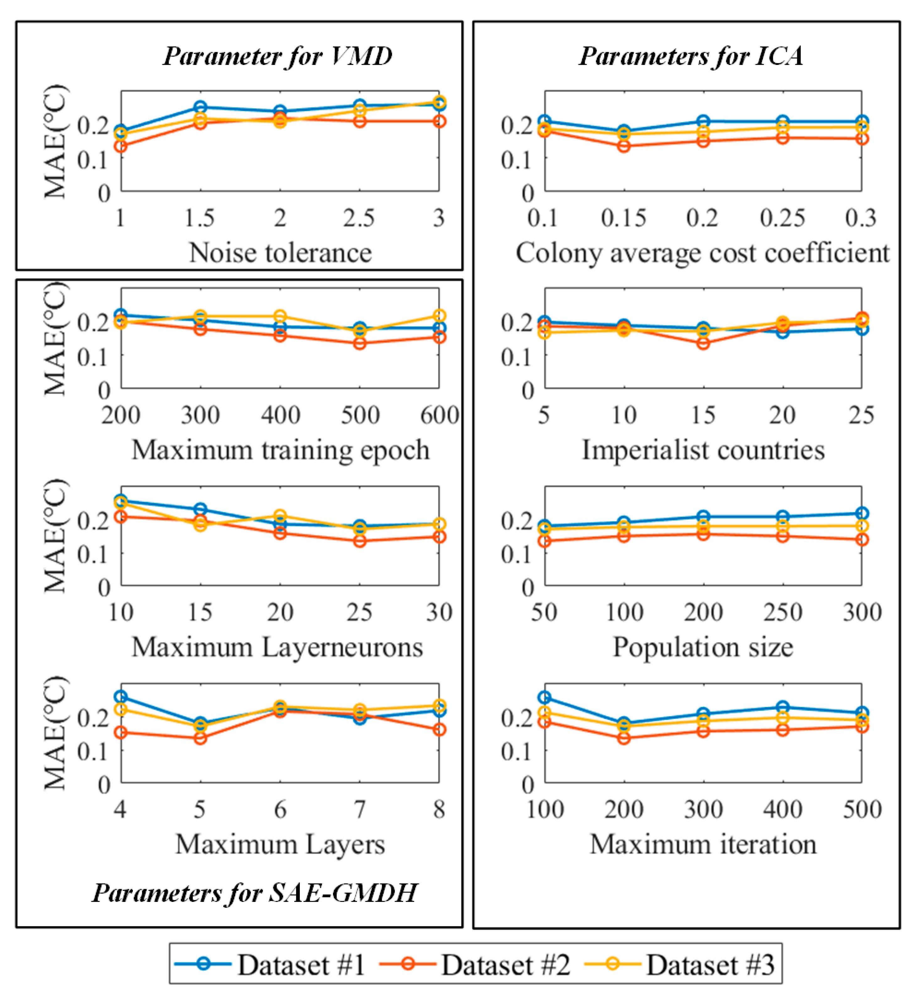
3.4. Sensitive Analysis of the Parameters and the Computational Time

In this section, the sensitivity of the parameters in the proposed model is analyzed. The parameters are tested by five different values. The sensitivity analysis results of the important parameters in the proposed model are presented in Figure 11. The MAEs are applied to represent the forecasting accuracy. It can be observed from the analysis results that the proposed model is generally stable and robust to the parameters with some fluctuations. For example, when the colony average cost coefficient is 0.2, the MAEs have the smallest values in all datasets, which means the best forecasting accuracy. As for the maximum iterations of ICA, the changing of the parameter value has little impact on the maximum iterations. To save computational time, it is rational to set the maximum iterations as 200. The optimal values of the important parameters are listed in Table 7.
The calculation cost of the proposed model is given. The forecasting process costs only a few seconds by measurement function in software Matlab and the data intervals are ten minutes. The training time is less than five minutes. The total computational time of the proposed models in the study is shown in Table 8. Therefore, real-time monitoring can be realized.

4. Conclusions and Future Work

The bearing temperature prediction can provide technical support for real-time failure detection in wind turbines. In this study, a novel hybrid prediction model, which is composed of a VMD, SAE, GMDH and ICA, is proposed for the bearing temperature of the gearbox in the wind turbine. The study can be concluded as follows:
(a) The VMD algorithm can greatly increase the forecasting accuracy by preprocessing and identification of raw data. The SAE can search for the deep information of decomposed data and avoid data redundancy, which can provide better input for the GMDH to improve the prediction ability. The proposed weight coefficient optimization method based on ICA is effective to raise the prediction accuracy and achieve better ensemble results compared with the traditional GA method.
(b) The proposed framework can deeply identify the fluctuation features of bearing temperature data to forecast the changing trend. The existing single predictors cannot extract deep nonlinear characteristics to establish accurate predictions, which can prove the robustness of the proposed model.
(c) Combining all advantages of the chosen algorithms, the proposed model proved to be better than other involved models and three state-of-the-art models, which has demonstrated its excellent forecasting power and applicability for bearing temperature time series. The datasets from the SCADA system present different temporal features and the proposed VMD-SAE-GMDH-ICA can provide an accurate prediction of normal changes and sudden rise or fall in bearing temperature.
The proposed model showed good predictive potential by the gearbox bearing temperature series, whose forecasted results can be embedded in relevant early detection and warning systems of wind turbine gearbox. For future work, more improvement may be carried out from the following aspects:
(a) The experiments of the proposed model are established by single time series forecasting. However, wind turbines are affected by many factors. Frequently updating the data to adjust the model parameters can effectively guarantee the model learning ability. After an effective establishment of fault detection and early warning system, other internal and external variables can be analyzed to improve system functions and expand the scope of research. In future work, the influence of other factors such as the ambient temperature and wind speed on bearing temperature is also worthy of study.
(b) The efficiency and effectiveness of the proposed framework have been confirmed in experiments. The real-time prediction model can be applied to detect the wind turbine status in advance, analyze the possibility of reaching the thresholds. Based on the existing algorithms, the scientificity and accuracy of the model need further improvement with lots of detection knowledge and problem-solved abilities for the actual application fields, such as the maintenance management by the external weather and output power [61,62], the risk assessment by the mechanical friction and internal and external temperature [62] and performance assessment [63].
(c) The simple time series prediction may not accurately present the overall fault diagnosis of the whole wind farms with multiple wind turbines. Therefore, the spatial-temporal forecasting model can be applied to improve this situation. The large amount of collected data that follow can be handled by big data platforms such as Spark to strengthen data processing power and to increase computing speed.

Author Contributions

Conceptualization, G.Y. and C.Y.; methodology, G.Y.; software, G.Y. and C.Y.; validation, G.Y.; formal analysis, G.Y.; investigation, C.Y.; resources, C.Y.; writing—original draft preparation, G.Y.; writing—review and editing, G.Y. and Y.B.; visualization, C.Y.; supervision, Y.B.; funding acquisition, Y.B. All authors have read and agreed to the published version of the manuscript.

Funding

This research received no external funding.

Acknowledgments

This study is fully supported by the National Natural Science Foundation of China (Grant No. 61902108) and the Natural Science Foundation of Hebei Province (Grant No. F2019208305).

Conflicts of Interest

The authors declare no conflict of interest.

References

  1. Zhang, D.; Wang, J.; Lin, Y.; Si, Y.; Huang, C.; Yang, J.; Huang, B.; Li, W. Present situation and future prospect of renewable energy in China. Renew. Sustain. Energy Rev. 2017, 76, 865–871. [Google Scholar] [CrossRef]
  2. Zhai, H.; Zhu, C.; Song, C.; Liu, H.; Bai, H. Influences of carrier assembly errors on the dynamic characteristics for wind turbine gearbox. Mech. Mach. Theory 2016, 103, 138–147. [Google Scholar] [CrossRef]
  3. Escaler, X.; Mebarki, T. Full-scale wind turbine vibration signature analysis. Machines 2018, 6, 63. [Google Scholar] [CrossRef] [Green Version]
  4. Ding, F.; Tian, Z.; Zhao, F.; Xu, H. An integrated approach for wind turbine gearbox fatigue life prediction considering instantaneously varying load conditions. Renew. Energy 2018, 129, 260–270. [Google Scholar] [CrossRef]
  5. Schlechtingen, M.; Santos, I.F. Comparative analysis of neural network and regression based condition monitoring approaches for wind turbine fault detection. Mech. Syst. Signal Process. 2011, 25, 1849–1875. [Google Scholar] [CrossRef] [Green Version]
  6. Ren, Z.; Verma, A.S.; Li, Y.; Teuwen, J.J.; Jiang, Z. Offshore wind turbine operations and maintenance: A state-of-the-art review. Renew. Sustain. Energy Rev. 2021, 144, 110886. [Google Scholar] [CrossRef]
  7. Yang, W.; Tavner, P.J.; Crabtree, C.J.; Wilkinson, M. Cost-effective condition monitoring for wind turbines. IEEE Trans. Ind. Electron. 2009, 57, 263–271. [Google Scholar] [CrossRef] [Green Version]
  8. Wang, L.; Zhang, Z.; Long, H.; Xu, J.; Liu, R. Wind turbine gearbox failure identification with deep neural networks. IEEE Trans. Ind. Inform. 2016, 13, 1360–1368. [Google Scholar] [CrossRef]
  9. Liu, Z.; Zhang, L. A review of failure modes, condition monitoring and fault diagnosis methods for large-scale wind turbine bearings. Measurement 2020, 149, 107002. [Google Scholar] [CrossRef]
  10. Li, Y.; Liu, S.; Shu, L. Wind turbine fault diagnosis based on Gaussian process classifiers applied to operational data. Renew. Energy 2019, 134, 357–366. [Google Scholar] [CrossRef]
  11. Stetco, A.; Dinmohammadi, F.; Zhao, X.; Robu, V.; Flynn, D.; Barnes, M.; Keane, J.; Nenadic, G. Machine learning methods for wind turbine condition monitoring: A review. Renew. Energy 2019, 133, 620–635. [Google Scholar] [CrossRef]
  12. Manobel, B.; Sehnke, F.; Lazzús, J.A.; Salfate, I.; Felder, M.; Montecinos, S. Wind turbine power curve modeling based on Gaussian processes and artificial neural networks. Renew. Energy 2018, 125, 1015–1020. [Google Scholar] [CrossRef]
  13. Astolfi, D.; Scappaticci, L.; Terzi, L. Fault diagnosis of wind turbine gearboxes through temperature and vibration data. Int. J. Renew. Energy Res. 2017, 7, 965–976. [Google Scholar]
  14. Zaher, A.S.A.E.; McArthur, S.D.J.; Infield, D.G.; Patel, Y. Online wind turbine fault detection through automated SCADA data analysis. Wind. Energy Int. J. Prog. Appl. Wind. Power Convers. Technol. 2009, 12, 574–593. [Google Scholar] [CrossRef]
  15. Zhu, L.; Zhang, X. Time Series Data-Driven Online Prognosis of Wind Turbine Faults in Presence of SCADA Data Loss. IEEE Trans. Sustain. Energy 2020, 12, 1289–1300. [Google Scholar] [CrossRef]
  16. Liao, T.W. Clustering of time series data—A survey. Pattern Recognit. 2005, 38, 1857–1874. [Google Scholar] [CrossRef]
  17. Moayedi, H.; Gör, M.; Foong, L.K.; Bahiraei, M. Imperialist competitive algorithm hybridized with multilayer perceptron to predict the load-settlement of square footing on layered soils. Measurement 2021, 172, 108837. [Google Scholar] [CrossRef]
  18. Song, L.-K.; Fei, C.-W.; Bai, G.-C.; Yu, L.-C. Dynamic neural network method-based improved PSO and BR algorithms for transient probabilistic analysis of flexible mechanism. Adv. Eng. Inform. 2017, 33, 144–153. [Google Scholar] [CrossRef]
  19. Xiao, Y.; Dai, R.; Zhang, G.; Chen, W. The use of an improved LSSVM and joint normalization on temperature prediction of gearbox output shaft in DFWT. Energies 2017, 10, 1877. [Google Scholar] [CrossRef] [Green Version]
  20. Xiao, X.; Liu, J.; Liu, D.; Tang, Y.; Dai, J.; Zhang, F. SSAE-MLP: Stacked sparse autoencoders-based multi-layer perceptron for main bearing temperature prediction of large-scale wind turbines. Concurr. Comput. Pract. Exp. 2021, e6315. [Google Scholar] [CrossRef]
  21. Abdusamad, K.B.; Gao, D.W.; Muljadi, E. A condition monitoring system for wind turbine generator temperature by applying multiple linear regression model. In Proceedings of the 2013 North American Power Symposium (NAPS 2013), Manhattan, KS, USA, 22–24 September 2013; pp. 1–8. [Google Scholar]
  22. Chen, S.; Ma, Y.; Ma, L.; Qiao, F.; Yang, H. Early warning of abnormal state of wind turbine based on principal component analysis and RBF neural network. In Proceedings of the 2021 6th Asia Conference on Power and Electrical Engineering (ACPEE), Chongqing, China, 8–11 April 2021; pp. 547–551. [Google Scholar]
  23. Fu, J.; Chu, J.; Guo, P.; Chen, Z. Condition monitoring of wind turbine gearbox bearing based on deep learning model. IEEE Access 2019, 7, 57078–57087. [Google Scholar] [CrossRef]
  24. Lu, L.; He, Y.; Ruan, Y.; Yuan, W. Wind turbine planetary gearbox condition monitoring method based on wireless sensor and deep learning approach. IEEE Trans. Instrum. Meas. 2020, 70, 1–16. [Google Scholar] [CrossRef]
  25. Wang, S.; Chen, J.; Wang, H.; Zhang, D. Degradation evaluation of slewing bearing using HMM and improved GRU. Measurement 2019, 146, 385–395. [Google Scholar] [CrossRef]
  26. Heydari, A.; Garcia, D.A.; Fekih, A.; Keynia, F.; Tjernberg, L.B.; De Santoli, L. A Hybrid Intelligent Model for the Condition Monitoring and Diagnostics of Wind Turbines Gearbox. IEEE Access 2021, 9, 89878–89890. [Google Scholar] [CrossRef]
  27. Yu, C.; Li, Y.; Xiang, H.; Zhang, M. Data mining-assisted short-term wind speed forecasting by wavelet packet decomposition and Elman neural network. J. Wind. Eng. Ind. Aerodyn. 2018, 175, 136–143. [Google Scholar] [CrossRef]
  28. Wang, S.; Zhang, N.; Wu, L.; Wang, Y. Wind speed forecasting based on the hybrid ensemble empirical mode decomposition and GA-BP neural network method. Renew. Energy 2016, 94, 629–636. [Google Scholar] [CrossRef]
  29. Gendeel, M.; Zhang, Y.; Qian, X.; Xing, Z. Deterministic and probabilistic interval prediction for wind farm based on VMD and weighted LS-SVM. Energy Sources Part A Recovery Util. Environ. Eff. 2021, 43, 800–814. [Google Scholar] [CrossRef]
  30. Khan, M.; Liu, T.; Ullah, F. A new hybrid approach to forecast wind power for large scale wind turbine data using deep learning with TensorFlow framework and principal component analysis. Energies 2019, 12, 2229. [Google Scholar] [CrossRef] [Green Version]
  31. Liang, Y.; Niu, D.; Hong, W.-C. Short term load forecasting based on feature extraction and improved general regression neural network model. Energy 2019, 166, 653–663. [Google Scholar] [CrossRef]
  32. Liu, J.; Li, Y. Study on environment-concerned short-term load forecasting model for wind power based on feature extraction and tree regression. J. Clean. Prod. 2020, 264, 121505. [Google Scholar] [CrossRef]
  33. Jaseena, K.; Kovoor, B.C. A hybrid wind speed forecasting model using stacked autoencoder and LSTM. J. Renew. Sustain. Energy 2020, 12, 023302. [Google Scholar] [CrossRef] [Green Version]
  34. Nie, Y.; Jiang, P.; Zhang, H. A novel hybrid model based on combined preprocessing method and advanced optimization algorithm for power load forecasting. Appl. Soft Comput. 2020, 97, 106809. [Google Scholar] [CrossRef]
  35. Zhang, W.; Maleki, A.; Rosen, M.A. A heuristic-based approach for optimizing a small independent solar and wind hybrid power scheme incorporating load forecasting. J. Clean. Prod. 2019, 241, 117920. [Google Scholar] [CrossRef]
  36. Wen, X. Modeling and performance evaluation of wind turbine based on ant colony optimization-extreme learning machine. Appl. Soft Comput. 2020, 94, 106476. [Google Scholar] [CrossRef]
  37. Li, Y.; Yang, F.; Zha, W.; Yan, L. Combined Optimization Prediction Model of Regional Wind Power Based on Convolution Neural Network and Similar Days. Machines 2020, 8, 80. [Google Scholar] [CrossRef]
  38. Yin, Z.; Gao, Q. A novel imperialist competitive algorithm for scheme configuration rules mining of product service system. Arab. J. Sci. Eng. 2020, 45, 3157–3169. [Google Scholar] [CrossRef]
  39. Afradi, A.; Ebrahimabadi, A. Prediction of TBM penetration rate using the imperialist competitive algorithm (ICA) and quantum fuzzy logic. Innov. Infrastruct. Solut. 2021, 6, 1–17. [Google Scholar] [CrossRef]
  40. Jaafari, A.; Zenner, E.K.; Panahi, M.; Shahabi, H. Hybrid artificial intelligence models based on a neuro-fuzzy system and metaheuristic optimization algorithms for spatial prediction of wildfire probability. Agric. For. Meteorol. 2019, 266, 198–207. [Google Scholar] [CrossRef]
  41. Dragomiretskiy, K.; Zosso, D. Variational mode decomposition. IEEE Trans. Signal Process. 2013, 62, 531–544. [Google Scholar] [CrossRef]
  42. Jayakumar, C.; Sangeetha, J. Kernellized support vector regressive machine based variational mode decomposition for time frequency analysis of Mirnov coil. Microprocess. Microsyst. 2020, 75, 103036. [Google Scholar] [CrossRef]
  43. Brzostowski, K.; Światek, J. Dictionary adaptation and variational mode decomposition for gyroscope signal enhancement. Appl. Intell. 2021, 51, 2312–2330. [Google Scholar] [CrossRef]
  44. Zhao, X.; Wu, P.; Yin, X. A quadratic penalty item optimal variational mode decomposition method based on single-objective salp swarm algorithm. Mech. Syst. Signal Process. 2020, 138, 106567. [Google Scholar] [CrossRef]
  45. Liu, Y.; Yang, G.; Li, M.; Yin, H. Variational mode decomposition denoising combined the detrended fluctuation analysis. Signal Process. 2016, 125, 349–364. [Google Scholar] [CrossRef]
  46. Zabalza, J.; Ren, J.; Zheng, J.; Zhao, H.; Qing, C.; Yang, Z.; Du, P.; Marshall, S. Novel segmented stacked autoencoder for effective dimensionality reduction and feature extraction in hyperspectral imaging. Neurocomputing 2016, 185, 1–10. [Google Scholar] [CrossRef] [Green Version]
  47. Adem, K.; Kiliçarslan, S.; Cömert, O. Classification and diagnosis of cervical cancer with stacked autoencoder and softmax classification. Expert Syst. Appl. 2019, 115, 557–564. [Google Scholar] [CrossRef]
  48. Mo, L.; Xie, L.; Jiang, X.; Teng, G.; Xu, L.; Xiao, J. GMDH-based hybrid model for container throughput forecasting: Selective combination forecasting in nonlinear subseries. Appl. Soft Comput. 2018, 62, 478–490. [Google Scholar] [CrossRef]
  49. Kim, D.; Seo, S.-J.; Park, G.-T. Hybrid GMDH-type modeling for nonlinear systems: Synergism to intelligent identification. Adv. Eng. Softw. 2009, 40, 1087–1094. [Google Scholar] [CrossRef]
  50. Hwang, H.S. Fuzzy GMDH-type neural network model and its application to forecasting of mobile communication. Comput. Ind. Eng. 2006, 50, 450–457. [Google Scholar] [CrossRef]
  51. Atashpaz-Gargari, E.; Lucas, C. Imperialist competitive algorithm: An algorithm for optimization inspired by imperialistic competition. In Proceedings of the 2007 IEEE Congress on Evolutionary Computation, Singapore, 25–28 September 2007; pp. 4661–4667. [Google Scholar]
  52. Geetha Devasena, M.; Gopu, G.; Valarmathi, M. Automated and optimized software test suite generation technique for structural testing. Int. J. Softw. Eng. Knowl. Eng. 2016, 26, 1–13. [Google Scholar] [CrossRef]
  53. Khanali, M.; Akram, A.; Behzadi, J.; Mostashari-Rad, F.; Saber, Z.; Chau, K.-W.; Nabavi-Pelesaraei, A. Multi-objective optimization of energy use and environmental emissions for walnut production using imperialist competitive algorithm. Appl. Energy 2021, 284, 116342. [Google Scholar] [CrossRef]
  54. Gordan, M.; Razak, H.A.; Ismail, Z.; Ghaedi, K. Data mining based damage identification using imperialist competitive algorithm and artificial neural network. Lat. Am. J. Solids Struct. 2018, 15. [Google Scholar] [CrossRef]
  55. Tien Bui, D.; Shahabi, H.; Shirzadi, A.; Chapi, K.; Hoang, N.-D.; Pham, B.T.; Bui, Q.-T.; Tran, C.-T.; Panahi, M.; Bin Ahmad, B. A novel integrated approach of relevance vector machine optimized by imperialist competitive algorithm for spatial modeling of shallow landslides. Remote Sens. 2018, 10, 1538. [Google Scholar] [CrossRef] [Green Version]
  56. Dao, P.B.; Staszewski, W.J.; Barszcz, T.; Uhl, T. Condition monitoring and fault detection in wind turbines based on cointegration analysis of SCADA data. Renew. Energy 2018, 116, 107–122. [Google Scholar] [CrossRef]
  57. Astolfi, D. Perspectives on SCADA Data Analysis Methods for Multivariate Wind Turbine Power Curve Modeling. Machines 2021, 9, 100. [Google Scholar] [CrossRef]
  58. Mi, X.; Zhao, S. Wind speed prediction based on singular spectrum analysis and neural network structural learning. Energy Convers. Manag. 2020, 216, 112956. [Google Scholar] [CrossRef]
  59. Dong, S.; Yu, C.; Yan, G.; Zhu, J.; Hu, H. A Novel Ensemble Reinforcement Learning Gated Recursive Network for Traffic Speed Forecasting. In Proceedings of the 2021 Workshop on Algorithm and Big Data, Fuzhou, China, 12–14 March 2021; pp. 55–60. [Google Scholar]
  60. Liu, X.; Qin, M.; He, Y.; Mi, X.; Yu, C. A new multi-data-driven spatiotemporal PM2. 5 forecasting model based on an ensemble graph reinforcement learning convolutional network. Atmos. Pollut. Res. 2021, 12, 101197. [Google Scholar] [CrossRef]
  61. Bangalore, P.; Patriksson, M. Analysis of SCADA data for early fault detection, with application to the maintenance management of wind turbines. Renew. Energy 2018, 115, 521–532. [Google Scholar] [CrossRef]
  62. Zhang, J.; Kang, J.; Sun, L.; Bai, X. Risk assessment of floating offshore wind turbines based on fuzzy fault tree analysis. Ocean. Eng. 2021, 239, 109859. [Google Scholar] [CrossRef]
  63. Bilal, B.; Adjallah, K.H.; Sava, A. Data-Driven Fault Detection and Identification in Wind Turbines Through Performance Assessment. In Proceedings of the 2019 10th IEEE International Conference on Intelligent Data Acquisition and Advanced Computing Systems: Technology and Applications (IDAACS), Metz, France, 18–21 September 2019; pp. 123–129. [Google Scholar]
Figure 1. The structure of the proposed model (A) decomposition method (B) improved predictor (C) optimization method.
Machines 09 00248 g001
Figure 2. Interval from the colony towards the imperialist.
Machines 09 00248 g002
Figure 3. The raw wind turbine bearing temperature series: (a) dataset #1 (b) dataset #2 (c) dataset #3.
Machines 09 00248 g003
Figure 4. Values of loss during the iterations of ICA and GA.
Machines 09 00248 g004
Figure 5. Forecasting results and errors of all models of series #1: (a) forecasting results; (b) error distribution; (c) local enlargement.
Machines 09 00248 g005
Figure 6. Forecasting results and errors of all models of series #2: (a) forecasting results; (b) error distribution; (c) local enlargement.
Machines 09 00248 g006
Figure 7. Forecasting results and errors of all models of series #3: (a) forecasting results; (b) error distribution; (c) local enlargement.
Machines 09 00248 g007
Figure 8. MAE results of eight models.
Machines 09 00248 g008
Figure 9. MAPE results of eight models.
Machines 09 00248 g009
Figure 10. RMSE results of eight models.
Machines 09 00248 g010
Figure 11. The sensitivity analysis results of the proposed model.
Machines 09 00248 g011
Table 1. The statistical results of the temperature time series #1, #2 and #3.
Bearing Temperature Time Series Temperature Time Series#1#2#3
Data resolution (min)101010
Minimum (°C)15.323.629.6
Mean (°C)28.276132.857343.1788
Maximum (°C)70.151.859
Standard derivation7.39625.62346.3141
Table 2. The error evaluation results of different predictors.
SeriesForecasting ModelsMAE (°C)MAPE (%) RMSE (°C)
#1GMDH0.36291.14170.6289
GRU0.46781.23880.6175
LSTM0.54751.05630.7308
DBN0.57941.56430.6396
ENN0.67061.61210.7831
ELM2.03743.64052.9887
GRNN1.15512.18201.6379
MLP0.84721.89560.9860
RBFNN0.71001.85390.9478
#2GMDH0.54650.70630.4372
GRU0.60530.73780.5128
LSTM0.62380.91280.7628
DBN0.59250.82900.5931
ENN0.62860.80700.6585
ELM0.82541.93520.8224
GRNN0.80021.23221.0628
MLP0.66841.05180.8478
RBFNN0.56720.81090.7466
#3GMDH0.52100.95910.7920
GRU0.64350.98410.9429
LSTM0.57981.27691.1923
DBN 0.55631.00560.8681
ENN0.73501.16081.0105
ELM0.83481.48731.2613
GRNN0.99412.05631.4930
MLP0.76631.43431.3829
RBFNN0.61981.22690.9243
Table 3. The promoting percentages of the SAE models.
MethodIndexesSeries #1Series #2Series #3
VMD-SAE-GMDH vs.
VMD-GMDH
PMAE (%)11.427617.186123.1070
PMAPE (%)18.500013.467917.3433
PRMSE (%)24.771429.241019.6399
SAE-GMDH vs. GMDHPMAE (%)21.686425.416320.3223
PMAPE (%)39.414921.951926.8168
PRMSE (%)31.276813.197625.1736
Table 4. The promoting percentages of the VMD-SAE-GMDH-ICA model by the VMD-SAE-GMDH-GA model and the VMD-SAE-GMDH model.
MethodIndexesSeries #1Series #2Series #3
VMD-SAE-GMDH-ICA
vs.
VMD-SAE-GMDH-GA
PMAE (%)11.100126.125119.5364
PMAPE (%)6.049311.799713.5180
PRMSE (%)21.682632.430913.2560
VMD-SAE-GMDH-ICA
vs.
VMD-SAE-GMDH
PMAE (%)30.492154.357438.1904
PMAPE (%)13.582519.392825.5384
PRMSE (%)28.864249.871852.1262
Table 5. The error evaluation results of different methods.
SeriesForecasting ModelsMAE (°C)MAPE (%)RMSE (°C)
#1GMDH0.36291.14170.6289
EMD-GMDH0.30041.02020.5077
EEMD-GMDH0.29581.00410.4179
VMD-GMDH0.29140.86000.3827
SAE-GMDH0.28420.69170.4322
VMD-SAE-GMDH0.25810.70090.2879
VMD-SAE-GMDH-GA0.20180.64470.2615
VMD-SAE-GMDH-ICA0.17940.60570.2048
#2GMDH0.54650.70700.4372
EMD-GMDH0.48840.66990.4088
EEMD-GMDH0.40230.56550.3577
VMD-GMDH0.35610.51010.3307
SAE-GMDH0.40760.55180.3795
VMD-SAE-GMDH0.29490.44140.2340
VMD-SAE-GMDH-GA0.18220.40340.1736
VMD-SAE-GMDH-ICA0.13460.35580.1173
#3GMDH0.52110.95910.7921
EMD-GMDH0.45550.88990.7637
EEMD-GMDH0.38310.86170.6047
VMD-GMDH0.35790.67980.5443
SAE-GMDH0.41520.70190.5927
VMD-SAE-GMDH0.27520.56190.4374
VMD-SAE-GMDH-GA0.21140.48380.2414
VMD-SAE-GMDH-ICA0.17010.41840.2094
Table 6. The promoting percentages of the EMD decomposition models and the VMD decomposition models.
MethodIndexesSeries #1Series #2Series #3
EMD-GMDH
vs. GMDH
PMAE (%)17.222310.631312.5887
PMAPE (%)10.64205.24757.2151
PRMSE (%)19.27176.49593.5854
EEMD-GMDH
vs. GMDH
PMAE (%)18.490026.386126.4824
PMAPE (%)12.025920.014110.1553
PRMSE (%)33.550618.183923.6586
VMD-GMDH vs.
GMDH
PMAE (%)19.702334.839831.3184
PMAPE (%)24.647527.850129.1211
PRMSE (%)29.147724.359643.9086
Table 7. The parameters with the optimal values by sensitive analysis.
ParametersValue
Noise tolerance1
Maximum training epoch500
Maximum Layerneurons25
Maximum Layers5
Colony average cost coefficient0.2
Imperialist countries10
Population size50
Maximum iteration200
Table 8. The main computational time of the proposed models.
AlgorithmsComputational Time
VMD7.823 s
SAE-GMDH155.794 s
ICA118.526 s
Total282.143
Publisher’s Note: MDPI stays neutral with regard to jurisdictional claims in published maps and institutional affiliations.

