Review

Data-Driven Intelligent 3D Surface Measurement in Smart Manufacturing: Review and Outlook

Department of Mechanical Science and Engineering, University of Illinois at Urbana-Champaign, Urbana, IL 61801, USA
*
Author to whom correspondence should be addressed.
Machines 2021, 9(1), 13; https://doi.org/10.3390/machines9010013
Submission received: 15 December 2020 / Revised: 7 January 2021 / Accepted: 8 January 2021 / Published: 13 January 2021
(This article belongs to the Section Advanced Manufacturing)

Abstract

:
High-fidelity characterization and effective monitoring of spatial and spatiotemporal processes are crucial for high-performance quality control of many manufacturing processes and systems in the era of smart manufacturing. Although the recent development in measurement technologies has made it possible to acquire high-resolution three-dimensional (3D) surface measurement data, it is generally expensive and time-consuming to use such technologies in real-world production settings. Data-driven approaches that stem from statistics and machine learning can potentially enable intelligent, cost-effective surface measurement and thus allow manufacturers to use high-resolution surface data for better decision-making without introducing substantial production cost induced by data acquisition. Among these methods, spatial and spatiotemporal interpolation techniques can draw inferences about unmeasured locations on a surface using the measurement of other locations, thus decreasing the measurement cost and time. However, interpolation methods are very sensitive to the availability of measurement data, and their performances largely depend on the measurement scheme or the sampling design, i.e., how to allocate measurement efforts. As such, sampling design is considered to be another important field that enables intelligent surface measurement. This paper reviews and summarizes the state-of-the-art research in interpolation and sampling design for surface measurement in varied manufacturing applications. Research gaps and future research directions are also identified and can serve as a fundamental guideline to industrial practitioners and researchers for future studies in these areas.

1. Introduction

Spatial and spatiotemporal processes are ubiquitous across all scales in manufacturing. They can manifest themselves in critical product quality characteristics (e.g., surface quality in machining [1,2,3,4], geometric compliance [5,6] and surface finish/texture [7] in additive manufacturing) or degradation of consumable tools (e.g., cutting and lapping tools in machining [8], horn and anvil in ultrasonic welding [9,10,11,12]). Figure 1 shows three examples of spatial and spatiotemporal processes in manufacturing at different scales and highlights the necessity of high-resolution surface measurement.
Figure 1a visualizes the deck face of a three-cylinder automotive engine head using high-resolution measurement data acquired by a laser holographic interferometer (LHI) with 300 μm lateral resolution [3,13,14]. Previously, the automotive industry had been using coordinate measuring machines (CMMs) for quality inspection of engine machining, but CMMs cannot adequately capture some small-scale variation patterns, e.g., the local distortions around the cylinder bores, which can be well characterized by the high-resolution surface measurement data acquired by LHI. Furthermore, the availability of such data has helped reveal new insights into the cutting dynamics and develop effective variation control methods, e.g., [1,2].
The topology of a degraded anvil surface, which was measured using a confocal laser microscopy (CLM), is shown by Figure 1b. Such measurements enabled the first studies on tool-wear characterization and monitoring in ultrasonic metal welding [10,15] and inspired a series of studies on data-driven surface modeling [11,16] and sampling design for spatiotemporal processes, e.g., [9,12]. Prior to these studies, industry practitioners had been using a conservative tool maintenance strategy based on the number of welding cycles, which led to a waste of tool life and/or deteriorated weld quality [15]. A deepened understanding of the tool degradation mechanism and effective tool condition monitoring technologies, e.g., [10,15], have promoted intelligent tool maintenance in ultrasonic metal welding.
Figure 1c displays the geometric measurement of six nanowires that were fabricated by two-photon lithography. An atomic force microscope (AFM) was used for the measurement. The designed wire height is 500 nm but the measurement data reveal that there is a systematic fabrication error, and this error depicts a spatial pattern. To date, there exists little research on the quantification and control of geometric errors in two-photon lithography. The availability of surface measurement data can potentially facilitate new research in quality assessment and control of two-photon lithography.
As seen from these examples, high-fidelity measurement and characterization of spatial and spatiotemporal processes cannot only reveal new insights into the physical processes but also inform effective decision-making to ensure the quality of processes and products. To enable this, high-resolution surface measurements are an imperative. However, the applications of high-resolution surface measurement systems in real-world manufacturing settings are still limited, mainly because of the prohibitive costs associated with the measurement process.
The costs of high-resolution surface measurement can be divided into direct and indirect costs. Direct measurement costs mainly include the capital and consumable costs of a surface measurement system. Many high-resolution measurement systems are costly, and the added value may not be obvious compared with the investment. Therefore, many manufacturers, especially small and medium-sized manufacturing companies, decide not to equip their production with such systems. Indirect measurement costs are mainly caused by the time-consuming measurement process. For example, the measurement in the examples shown in Figure 1b,c takes 45 min and 3 h, respectively. In addition, some measurement systems require careful calibration, removal and transport of products or production tools, and postprocessing of the raw measurement data, all of which introduce delays to the decision-making process that depends upon these data. The delayed decision-making leads to undesirable outcomes including reduced production rate and deteriorated product quality.
Intelligent, cost-effective surface measurement is critically needed to overcome these limitations. Data-driven interpolation methods for spatial and spatiotemporal processes draw inferences about unmeasured locations on a surface from the measurement of other locations as well as other sources of information; thereby, they cost-effectively generate high-resolution surface data from low-resolution data. However, to ensure satisfactory interpolation performance, one must choose a proper measurement scheme or sampling design, namely how to adaptively allocate measurement efforts, because interpolation methods are very sensitive to the availability of measurement data. As such, surface interpolation and sampling design are considered to be important driving forces of intelligent 3D surface measurement.
Surface interpolation and sampling design were more popularly investigated in non-manufacturing areas such as ecology (e.g., [17,18]), environmental science (e.g., [19,20]), and geology (e.g., [21]). In the past decade or so, the increasing adoption of high-resolution measurement data in smart manufacturing decision-making, e.g., quality monitoring, process control, maintenance has greatly promoted research in the manufacturing community [22,23]. Most manufacturing research on these topics either directly applies existing methods that were originally developed in other fields or extends them to address the unique challenges in manufacturing applications. To the best of our knowledge, while relevant manufacturing research has become more active, there is no systematic review that summarizes the recent advances or suggest future research directions. Furthermore, the implementation of the published methods in factory-floor settings is still inadequate. As such, this paper aims to provide a timely review of the state-of-the-art research in intelligent surface measurement. The specific goals of this review include the following.
(1)
To help industry practitioners choose the most appropriate measurement system and data-driven methods for enhancing the cost-effectiveness of surface measurement;
(2)
To identity the key gaps between academic research and industrial practice; and
(3)
To determine the critical research gaps and suggest future research directions.
The remainder of this paper is organized as follows. Section 2.1 summarizes the most commonly used 3D surface measurement techniques in manufacturing and measurement system analysis (MSA) for such techniques. Section 3 and Section 4 review existing data-driven interpolation and sampling design methods for surface measurement. Methods that have excellent potential but have not been applied to manufacturing surface measurement are also included. Then Section 5 summarizes the research gaps and presents suggested future research directions. Finally, Section 6 concludes the paper.

2. 3D Surface Measurement Techniques

This section first summarizes, analyzes, and compares the commonly applied 3D surface measurement techniques in manufacturing, including CMM, AFM, CLM, LHI, and structured light scanner (SLS), and then discusses the MSA of such techniques.

2.1. Measurement Instrument

Various surface measurement instruments have been adopted in manufacturing. In general, the surface measurement instruments can be classified as contact type and non-contact type, depending on the technologies behind them. A comparison of the contact and non-contact surface measurement systems based on the discussion in [24,25] is provided in Table 1.
In general, a contact or tactile measurement instrument equips a moving system with high-precision position sensors, which carries a touching probe. Such an instrument is also known as stylus-based instrument. The working principle of contact measurement systems is based on a mechanical interaction with the workpiece. Contact measurement system can achieve ultra-high measurement precision because of its nature of physical contact, and it is the only possible choice when highest precision is required. Because the touching probes contact with or move along the object surface, the workpiece can be damaged and modified inevitably and irreversibly. The contact may also wear or damage the tools, and the replacement of probes or styluses could cause an expensive maintenance cost [24,26].
Overcoming some of the shortcomings of contact surface measurement systems, non-contact surface measurement instruments become an irreplaceable choice for measuring complex surfaces at high speed with richer quantitative information. Neither the part surface nor the microscope is likely to be damaged as there is no physical contact between them. It is the only possible measurement approach for very soft or very hard surfaces. Additionally, the scanning rate of the contact systems is limited by the physical movement of tools. These physical constraints make contact systems disqualified for some high-throughput manufacturing applications in an industrial environment. However, the ultimate resolution of most optical measurement systems is limited due to the physics of diffraction. They can be lured by the optical properties of a sample, such as highly reflective and transparent [25]. Under these circumstances, the reflected light can be reduced or scattered uncontrollably. Prepossessing the challenging surfaces, e.g., using powdered spray-based coating, may be necessary for improving the measurement capability [27,28]. Nevertheless, the influence of the selected surface pre-processing and other environmental factors, e.g., lightning conditions, needs to be thoroughly investigated [25].
Although the measurement techniques falling under the same category, contact or non-contact, share similar advantages or disadvantages, each technique has its own characteristics and applications. In this section, we introduce five commonly used surface measurement systems and discuss examples of their applications in manufacturing. Figure 2 shows the typical measurement ranges and resolutions for these measurement technologies.

2.1.1. CMM

CMM is recognized as the first modern 3D surface measurement system [29,30]. Because the measurement process is facilitated through physical contact between a stylus and workpiece surface, CMM is categorized as a contact measurement instrument. The measurement resolution of CMM depends on the tip radius, because the interaction with the workpiece causes a mechanical filtering of the surface and the measurement could be a smoothed approximation of the sharp edges or peaks on the surface. An ultra-precision micro-CMM can achieve a measurement resolution at the order of nanometers [26]. It should be noted that as the measurement speed of CMM increases, dynamic errors can become much larger and the measurement accuracy may be adversely impacted [31].
As shown in Figure 2, CMM can work on varied measurement ranges and resolutions. CMM has seen wide applications in manufacturing. For example, Jin et al. employed a touching probe CMM to monitor the geometric quality of sliced wafers in wafer cutting processes [32]. Santos et al. adopted CMM for inspection of dimensional properties of parts manufactured through additive manufacturing [33]. Jiang et al. investigated the data processing techniques to improve high-precision reverse engineering with CMM measurement [34]. In addition, CMM has been widely used to evaluate the quality of machined surfaces [3,4,35].

2.1.2. AFM

AFM is a type of scanning probe microscopy that can provide atomic resolution for topographic imaging [36]. A typical AFM probe consists of a cantilever and a sharp tip fixed at the end of a cantilever. AFM can also work in non-contact mode. The cantilever is oscillated at its resonant frequency with amplitude of a few nanometers, and the tip of the cantilever does not contact the sample surface. The surface topography can be measured by recording mechanical resonance oscillation of the cantilever. Although it can be operated in both contact mode and non-contact mode, it is often considered to be a contact surface profiler because the surface dimensions are reflected by the interaction between the sample and the sharp tip.
AFM is one of only a few options of measurement instruments that can achieve a vertical measurement resolution on the order of fractions of a nanometer, which is far beyond the diffraction limit in the optical systems. Although its measurement range is limited, AFM is uniquely suitable for surface topography in nano-manufacturing and nano-mechanics [36,37]. In addition, AFM has the advantage of imaging almost any type of surface, including polymers, ceramics, composites, glass, and biological samples [38]. For example, Mwema et al. used AFM to examine the evolution, roughness and distribution of surface structure in a thin film deposition process [37].

2.1.3. CLM

Unlike some other optical imaging techniques, CLM can achieve resolution that is below the diffraction limit [39,40]. CLM measures a workpiece surface using vertical scanning and detects the intensity peak for each pixel. High-intensity peaks are generated by areas lying exactly in the focal plane. This feature enables CLM to achieve a high axial resolution as well as a high signal-to-noise ratio in the final measurement.
As shown in Figure 2, CLM has the highest resolution among the optical measurement systems, making it a good choice for accuracy-sensitive applications with a relatively small measurement area. It has been widely used for nano- and micro-scale surface characterization studies, e.g., evaluating the effects of machining and polishing techniques on surface topography [41,42,43], analyzing the geometric characteristics of products in additive manufacturing [5], assessing fatigue damage in mechanical structures [44], and monitoring the tool-wear progression in ultrasonic metal welding [9,10,11,12].

2.1.4. LHI

LHI is a two-step measurement technique combining laser interferometry and holography. In the two-step process, a digital holographic interference pattern is generated and split into a reference beam and a measurement beam, and then the beams returned from the target surface is merged and recorded simultaneously. The recorded hologram of the target surface carries both the amplitude and phase of the returned beam, and the surface can be reconstructed based on it [45,46]. Because LHI relies on the phase shift measurement, it can only achieve vertical resolution at hundreds of nanometers and lateral resolution at micrometers.
LHI is a great fit for characterization of micro-scale topography features. In semiconductor industry, it has been adopted for defect detection of semiconductor materials in the deposition and etching process [47,48]. In automotive industry, applications include monitoring engine head surface and press formed parts such as outside door panels [13,14,49].

2.1.5. SLS

SLS projects light patterns on the target surface, which is similar to LHI. During the SLS measurement process, multiple patterns of non-coherent light are projected and subsequently elaborated to obtain the range information from each viewed point [50,51]. Recently, SLS has received increasing attention because it has a relatively fast measurement speed and a large measurement range (see Figure 2). Within a few seconds or even in real time, SLS can scan a broad field with measurement range up to a few meters. However, high inspection speed and large measurement range of SLS are possible at the cost of sacrificing its spatial resolution. For 3D surface measurement applications that require high-speed or even real-time monitoring over a wide field of view, SLS is an excellent choice [50].

2.2. MSA

It is important to calibrate, verify, and validate a measurement system to ensure the fidelity of measurement data prior to using them in production decision-making. MSA uses a series of tools including design of measurement experiments and statistical methods to identify the amount of variation that exists in a measurement process [14,52]. Classical MSA theory assumes that the measurement variation can be decomposed into two components of variation—repeatability and reproducibility (R&R). Accordingly, gage R&R studies are deemed as a major MSA tool.
Despite being developed for low-dimensional measurement data, classical MSA methods and their extensions have been used for surface measurement data, which are normally of much higher dimension. Figure 3 shows a general MSA procedure for surface measurement data. Data pre-processing is a necessary step prior to the subsequent analysis. The acquisition of high-resolution measurements may be interfered by environmental disturbances, such as machine vibration, heat dissipation, and surface contamination [49]. Because these environmental factors could cause data loss and distortion, data interpolation and de-noising should be performed. Additionally, the raw surface measurement data is a collection of 3D points, where each point is identified by an ordered triple ( x , y , z ) . Prior to analyzing multiple repetitive measurement data, it is preferable to align and transform the raw data to one common coordinate system, which has a regular, rectangular grid in the x - y plane, and the measured points are differentiated from each other by height information in the z-axis. This process is known as point registration or point regularization. Registration is one necessary and decisive pre-processing step prior to the following analysis, especially when different numbers of points in different locations are produced from the measurement systems, which is commonly seen in optical surface measurement systems [14].
Currently, conventional capability indices have been adopted by most industry practitioners to quantify the performance of a measurement system. In these MSA models, the total measurement variation is decomposed into several measurement system components, such as the variance of the true but unknown value of the quality characteristic, the inherent gage precision (or repeatability), and operator variation (or reproducibility). The variation components can be estimated by two-way analysis of variance (ANOVA) [52].
Although these conventional methods are straightforward and intuitive to use in practice, they can only assess the system capability from individual quality characteristics. In other words, only univariate capability indices are used. However, multiple capability indices with quality characteristics of a high-resolution surface measurement system can be highly correlated [14]. The correlations between quality characteristics should be measured statistically, and correlated quality characteristics should be investigated jointly. In addition, because the global or dimensional quality characteristics might not reflect the local variations in the surface measurement, which can be spatially correlated, the system capability could be estimated inaccurately with conventional indices. A localized areal MSA, which aims to characterize measurement systems at local areas and locate the areas where the gages are not capable, is desired for high-resolution measurement systems.
Two types of strategies have been devised recently for dealing with the challenges in high-resolution measurement data. A multivariate extension of ANOVA—Multivariate analysis of variance (MANOVA)—was adopted in some works to calculate the capability indices across multiple dimensional characteristics, e.g., [53]. Nevertheless, when directly applied to the surface measurement data, MANOVA suffers from a lack of degree of freedom when the number of data dimensions is larger than the number of observations, which is often the case for high-resolution measurement data. To tackle this challenge, reduction of data dimensionality can be performed to extract the most significant features from the original measurement data. Both key product quality characteristics, e.g., overall flatness, regional flatness, and surface roughness in machined engine blocks, and data-driven features, e.g., principal component scores from principal component analysis [54] have been used.
ANOVA-based and MANOVA-based MSA do not characterize measurement systems at local areas. To accurately estimate gage capability of measuring local variations, pointwise MSA and spatial clustering MSA approaches has been developed to provide information about the spatial distribution of gage capability [14]. By preserving the spatial surface variations, the point-based and clustering-based approaches can characterize measurement systems at local areas and locate the regions where the gages are not capable.

3. Interpolation Method

Once measurement data have been obtained from instruments, they generally need proper treatment before being used for decision-making. Interpolation methods serve as a basic tool for both data enhancement and conversion between different data formats. In this paper, we define “interpolation” as follows: with available relevant information, an interpolation estimates the value of a function f at locations in a subset D R n ( f : D R representing the distribution of the quantity over a space D). In the context of surface measurement, f usually represents the surface topography, which is the height function over a region D R 2 over the surface. Here, we only sketch the basic theoretical outline of interpolation methods in the broader sense, which were developed in different fields, and are brought together for the first time in this review, to demonstrate their underestimated potential for manufacturing surface quantification.
The rest of this section is organized as follows. We first introduce a classification framework for interpolation methods in Section 3.1. Brief description of representative methods in each type with references is provided in Section 3.2, Section 3.3 and Section 3.4. Finally, the applications of the interpolation methods in manufacturing are briefly discussed in Section 3.5.

3.1. Classification Framework

A basic classification framework for interpolation methods is provided in Table 2. We will describe this classification system in this subsection, with clarification about some term usage.
We first make precise the meaning of aforementioned “available relevant information” for interpolation. Such information should at least contain a set of M measurements of the primary variable f: O = { y i = l i ( f ) + e i , i = 1 , , M } , where l i are functionals over a function space from the domain D R , and e i is the error of the i-th measurement. A measurement l i is exact if l i is equal to the evaluation functional at some x i D , or equivalently l i ( f ) = f ( x i ) . When f represents surface topology, such exact measurements are heights f ( x i ) of the surface at the sampled locations { x i , i = 1 , , M } D . Relevant information could also include a set { O α , α A } of sets O α = { ( x j α , f j α ) D × R , j J α } , which contain values of some relevant quantities f α in a family parametrized by α , associated with coordinates via proper registration procedures. f α with different α could represent different relevant quantities (attributes) with different parameters, time, batch, etc. In the context of surface measurement, such relevant information could be an optical image of the surface, vibration signals during its machining process, topology measurements of the previous surface in the production line, and so on.
Depending on whether D is continuous or discrete, interpolation methods fall into two main categories: continuous variation where D is a continuous region, and discrete variation where D is a discrete set. Methods for continuous variation could be further classified to two sub-classes: (1) spatial-only methods only make use of spatial data, including samples of the primary variable and coordinates as explanatory variables; while (2) data fusion methods also incorporate external information that is not spatial.
Most of times, methods for discrete variation deal with cases where D is a lattice. Categorization of these methods depends largely on the fields that the methods were developed. Methods in spatial statistics tend to use a discrete stochastic process to model the function, while those developed in image super-resolution and compressed sensing (in computer science and signal processing societies) stress on using a reduced number of (partial) measurements. Such distinctions are not absolute, as many methods could be transferred between different fields.
To use discrete interpolation methods, one may discretize the space to construct a fine (usually regular) grid; after proper registration, measurements performed at a coarser scale than the grid size are modeled as a certain function of values of f over localized clusters of grid vertices. These measurements, together with the measurement model and prior information about the behavior of f over the grids, are used to recover the values of f over the fine grid.
For almost all continuous methods, measurements of the primary variable must be exact, i.e., O = { f ( x i ) + e i , i = 1 , , M } , where x i D . Spatial-only methods deal with only O that has statistically homogeneous (most of times, i.i.d.) error e i ; and other cases need to be addressed by data fusion methods to take more factors into account. Discrete methods may take more general measurements, e.g., linear measurements l i ( f ) = j c j i f ( x i ) of certain type, as will be discussed in Section 3.4.

3.2. Spatial-Only Methods for Continuous Variation

According to different views adopted naturally for spatial-only methods, there are three types of approaches: the first deals with sampling or approximation/fitting problems within certain class of functions; the second one essentially makes inference about relevant spatial stochastic field; and the remaining methods could not be well-fitted into the previous two types, and depend more on the concept locality. Table 3 provides a classification of these methods. We note that this classification is not absolute, since one method might be viewed from different angles. We will further clarify on this matter at the end of this subsection.

3.2.1. Sampling or Approximation in Certain Class of Functions

Methods in this class generally selects an element f ^ in a function class V, according to certain criteria with corresponding algorithm. The criteria involve conditions characterizing how well f ^ fits the data y i f ( x i ) in O, where { x i } i = 1 M D . Other possible components for such criteria include goodness of f ^ ’s behavior in some sense, and additional constraints for f ^ . Essentially, it should produce a unique element with the criteria specified.
The criterion for the sampling problems is roughly the constraint that f ^ is an interpolant, i.e., f ^ ( x i ) = y i , which uniquely determines an element f ^ in V. It should be noted that here “sampling” refers to the reduction of a continuous (analog) signal into a discrete set of values, which is commonly seen in the signal processing context. In many sampling theories, it is of great interest to determine (1) when a function f V could be uniquely determined by its values over a discrete set, (2) how it could be reconstructed from these values, and (3) how well the reconstruction result is, in the presence of noise, or when f V and reconstruction produces some projection f ^ of f on V. By answering these questions, interpolation could then be performed with the reconstruction method specified by relevant sampling theorems, recovering an f ^ f from O.
As for approximation or curve fitting problems, the criteria are usually expressed in terms of a loss function J ( f ^ , O ) , which is minimized by f ^ ; sometimes f ^ is subject to additional constraints C. The solution f ^ is supposed to be unique. Most of the time, the loss function is of the form
J ( f ^ , O ) = d ( f ^ , O ) + λ R ( f ^ ) ,
where d ( f ^ , O ) measures the discrepancy between f ^ and data O, the regularization term R ( f ^ ) captures the “complexity” of f ^ , and λ balances the two factors.
The remainder of this section will introduce several representative interpolation methods that fall into the category of sampling or approximation, and could be classified according to the associated function space V and relevant criteria.

In Shift-Invariant Space: Sampling Theory

When V is some shift-invariant function space, interpolation could be addressed with relevant sampling theories [55]. The shift-invariant space V = V p ( ϕ ) is in the form of
V p ( ϕ ) = k Z d c k ϕ ( · k ) : c p ,
where l p = { c = ( c k ) k Z d | c p < } is the p-th summable sequence space, and c p = ( k Z d | c k | p ) 1 / p . It could be roughly understood as a linear function space spanned by the translation of the generator ϕ : R n R to the integer grid.
According to the theorems in [55], given data that is sampled sufficiently densely, the function f could be stably reconstructed via the iterative algorithm proposed. When f is not in V, the reconstruction results in certain projection of f to V with bounded errors. In particular, when ϕ ( x ) = sin c ( x ) = sin ( π x ) / ( π x ) and p = 2 , it contains the Paley-Wiener space of functions bandlimited to π as a special case, and reproduces the classical result of Shannon’s [56] after proper rescaling: f could be exactly recovered from uniform samples of period T via
f ( x ) = k Z f ( k T ) sin c ( x / T k ) ,
when f ( x ) is bandlimited to the Nyquist frequency π / T .
By specifying different generators, we may adjust properties of the function space to suit different requirements. The tensor product ϕ n = ϕ 1 ϕ 1 of 1D generators ϕ 1 is commonly used in multi-dimensional cases. Also note that the domain of the function is the entire space R n , so proper extension (padding) is usually required.
When samples are taken exactly over the integer grid which is used to define the shift-invariant space, i.e., the uniform sampling case in classical theory [56,57], the interpolation could be much more efficiently implemented by a convolution with corresponding interpolation kernel ψ . Such formulation further facilitates straightforward analysis in the frequency domain. It then becomes clear that interpolation in terms of sampling results in aliasing and low-pass filtering, which come from information loss in the data acquisition phase and convolution with the interpolation kernel ψ , respectively.
Such interpolation techniques for uniform sampling are widely applied in different signal processing scenarios, e.g., image interpolation [57]. In more general cases, relevant sampling theories still serve as standard practices and provide basis for data acquisition and processing procedures.

In RKHS: Regression with L2 Regularization and RBF Interpolation

Methods of this type essentially specify a proper kernel function k : D × D R , and find approximation of the data O in a function space V = H determined by k, by minimizing loss function J ( f ^ , O ) = d ( f ^ , O ) + R ( f ^ ) . H is the native semi-Hilbert space [58,59] of the conditionally positive definite (p.d.) kernel k (regarding a finite-dimensional function space P). The space H has an RKHS subspace with reproducing kernel induced by k. Most of times, P consists of polynomials lower than a certain order. When P = { 0 } , k is called a p.d. kernel, and H is the RKHS with reproducing kernel k. The discrepancy d ( f ^ , O ) is taken to be the mean squared error (MSE) and the regularization R ( f ^ ) = f ^ H 2 works with the semi-norm · H in H. Then, the solution f ^ of arg min f ^ H { 1 M i = 1 M ( f ^ ( x i ) y i ) 2 + λ f ^ H 2 } can be found in the form f ^ = p + i = 1 M α i k ( · , x i ) , where p P .
Methods in this class essentially differ from each other by the kernel they use. Commonly used p.d. kernels in statistical learning (e.g., polynomial kernel, Gaussian kernel, Laplacian kernel) are all applicable for such regularized regression or interpolation. Another class of examples is provided by splines defined by variational problems which could be related with RKHS’s [60,61]. For example, by penalizing s-th order derivatives, we could get polyharmonic splines in R n , for which the kernel is k ( x 1 , x 2 ) = k ( r ) , r = | x 1 x 2 | , x 1 , x 2 D , where k ( r ) r 2 s n log r for 2 s n even, k ( r ) r 2 s n for 2 s n odd. This kernel is conditionally positive definite regarding the space P of polynomial of order less than s 1 . Letting s = 2 , n = 2 , we get the most common 2-D thin-plate spline.
RBF interpolation methods also fall into this category. This corresponds to the case when the kernel k = k ( r ) is a radial function, and the penalty λ 0 so that the approximation produces an interpolant. Except the Gaussian kernel and smoothing splines, most commonly used kernels for RBF interpolation also include (Hardy’s) multiquadric r 2 + c 2 (for which P consists of linear polynomials), inverse multiquadric 1 / r 2 + c 2 , and compactly supported functions of minimal degree defined in [58], the latter two being positive definite. Interested reader could refer to [58,62] for more about RBF interpolation.

Other Methods for Approximation or Curve Fitting

It is also common to adopt function spaces and relevant criteria which are different from those of previous sampling and RKHS-related methods. This leads to various techniques for curve fitting, which are common in the statistical learning literature, and widely used for to process various data.
The function class V could take various forms. One of the most basic and commonly seen cases is when V is a linear space spanned by an explicitly given basis { ϕ j } j = 1 N . Accordingly, f ^ = β j ϕ j for some β = ( β j ) R N . Specifying different basis results in different function classes. A generalized linear model (GLM) is obtained when some nonlinear link function is used to transform V. The most important parametrized curve families for surface interpolation are B-splines and non-uniform rational basis spline (NURBS), which have found a wide application and become a fundamental tool in the field of computer-aided design, computer-aided manufacturing, and computational geometry [63]. To approximate a 2.5D surface which is regarded as a function, it is a common practice to form the basis using cubic (forth-order) B-splines with prescribed knots and fit following the standard least-squares (LS) procedure, while fitting general 3D surfaces with these curve families is more complicated [64]. Please note that B-splines could also be used to yield interpolants, see [65] for example.

3.2.2. Inference about Spatial Stochastic Fields

Methods in this class often use probability models that involve a continuously indexed spatial process, and assume the observed data are sampled from a realization of the stochastic process model [66,67]. Such models often take the form of
Y = f + ϵ ,
f = μ + η ,
where μ accounts for the mean of the stochastic process as “trend”, η is a zero-mean spatial process characterizing the local variation, and ϵ is the measurement error. The surface is regarded as a realization of the model f, and observed data O = { Y ( x i ) } contains measurements of this realization at locations x i . To interpolate at location x, we make use of the correlations between f ( x ) and Y ( x i ) ’s, both of which are random variables, to obtain some estimator for f ( x ) in terms of Y ( x i ) ’s.
In most cases, we may assume the process η has a finite covariance. Under this assumption, the most classical estimator is the best linear unbiased predictor (BLUP), known as universal kriging in the spatial statistics literature. It is assumed that μ = Φ β is the linear combination of a deterministic function basis Φ = ( ϕ 1 , , ϕ N ) , and η and ϵ are independent from μ with known covariance. Letting Φ be zero or constant, simple or ordinary kriging could be treated as special cases. When Φ contains basis functions other than polynomials, and sometimes linked with other regression methods via transformation, it is often referred to as regression kriging [68]. Another common variant is to perform regression with an arbitrary tool, and perform kriging over the residues. Such practice is more common in data fusion methods that will be discussed in the next section. There are other variants of kriging to suit different types of data, especially for geoscience and environmental science applications, but they are less common for interpolating surfaces and therefore omitted in this paper. Reviews [69,70] have more details regarding different kriging variants and combined methods.
The covariance required for kriging is generally specified by a parametrized covariance (or variogram) function fitted to measurement data. Refer to [66] for a detailed discussion on this topic. Yang et al. [11] provided an example for selecting a proper variogram to suit a specific engineering surface interpolation task.
The simple linear form of the kriging-type estimators results in a weak assumption on the field and usually tractable explicit solution. When the process is a Gaussian process (GP), the BLUP coincides with the conditional mean (given observations) and is indeed the best unbiased predictor. This procedure is often termed Gaussian process regression (GPR). Thus, when using these methods, we are either making a weak assumption regarding the process but restrict to linear estimators, or imposing a strong assumption that the process is a known Gaussian field. It is known that BLUP could lead to poor result in non-Gaussian case (see examples in [71]). Such failure could then be interpreted either as the limitation of the linear form, or nonconformity with the Gaussian assumption.
More recent research in spatial statistics tends to adopt the second view [66], i.e., assuming the process is completely specified by the model, and constructing estimators from the Bayesian point of view. Universal kriging, from this point of view, is the conditional mean given observations, when process η is stationary Gaussian with a known covariance function and prior on coefficients β is improper. Parameters for this covariance are usually estimated with likelihood-based methods. For basic generalization, hierarchical models [66,72] are often used to construct the process model from GPs and parameter priors. Inference is then made by analyzing relevant posteriors. This is sometimes termed as Bayesian kriging [73]. Further generalizations involves modeling of non-stationary [74,75] or non-Gaussian fields [66,73]. Also, Bayesian estimator for more complicated models generally does not take a closed form; such inference procedures usually require more modern tools (e.g., Monte Carlo algorithm) developed for statistical inference.

3.2.3. Other Methods for Spatial Interpolation

Mesh-Based Methods

Mesh-based interpolation methods depend on mesh structure associated with the measured locations { x i } i = 1 M . Based on the type of mesh required for setting up the interpolation, we further categorize them and list the main methods as follows. These methods are also reviewed in some other places, e.g., [70,76].
(1)
Voronoi tessellation: nearest-neighbor interpolation and natural neighbor [77] interpolation.
(2)
Triangular tessellation: triangular mesh is usually generated based on Delaunay triangulation. Within each triangular cell, linear (or piecewise cubic) function is selected to meet the interpolant constraint (and smoothness constraints) [76].
(3)
Rectangular grid: methods that rely on rectangular grid could actually fit into the previous types, including sampling theories and B-spline related methods, thus not to be repeated here.

Local Regression Methods

These methods usually perform weighted LS with a set of basis and weight specified by a weight function [78,79]. When the basis contains only constant, these methods yield a weighted average, reproducing kernel regression/smoothing with the weight function. Inverse distance weighting [80] could be viewed as a special case of local regression, when the weight function possesses some singularity.

3.2.4. Relationships between Aforementioned Spatial-Only Methods

Connection between Kriging, GPR and RKHS Regression Methods

It is well-known that a second order stochastic process generates a Hilbert space, which is congruent to an RKHS with the covariance function as reproducing kernel [60,81]; from this point of view, BLUP is equivalent to orthogonal projection in that RKHS.
When the process is further Gaussian, one may always find a function space so that it is equipped with a Gaussian measure (congruent to that of the GP), and in which the previous RKHS is densely embedded [82]. From this point of view, restricting the Gaussian measure to that RKHS, a GP imposes a kind of “prior” on functions in it, with the corresponding log-likelihood proportional to the RKHS norm. Performing GPR is equivalent to selecting the most likely function (regarding given data) in an RKHS, which means having minimal RKHS norm.
Interpreting GPR as regression in RKHS could allow us to perform a relatively “fair” comparison between interpolation with spatial process method and with the sampling or approximation in function classes; at least one may compare if the function space adopted could well characterize the underlying truth of f.

Effect of Aliasing and Low-Pass Filtering for Linear Interpolation Methods

Most of the previously discussed interpolation methods are linear: once measured locations are specified, the resulted estimator is a linear function of function values at these locations. Then, when the measurements are taken over the integer grid, it could be shown [57] that the estimator could be written as a convolution with certain equivalent interpolation kernel. From this point of view, aliasing may happen if the samples are not sufficiently dense. This leads to information loss, depending entirely on sampled locations. Then, different interpolation methods correspond to linear low-pass filters with frequency characteristics determined by equivalent interpolation kernel. This could be viewed as a drawback of linear interpolation methods, implying that they are neither able to perform de-aliasing, nor faithfully restore higher-frequency information.

3.3. Data Fusion-Based Interpolation for Continuous Variation

In a general perspective, data fusion is the process of integrating observations from multiple data sources to generate more robust, accurate, and meaningful information than that provided by each individual data source. In the context of surface measurement, data fusion uses multi-source information to acquire an accurate characterization of the surface of interest, with goals of improving the interpolation performance and reducing the measurement cost. Possible data sources include relevant but different attributes, temporally correlated measurements, knowledge of measurement instrument, and data from similar processes, as illustrated in Figure 4. In this section, we will review four data fusion methods developed for the interpolation of continuous variation.

3.3.1. Interpolation with Multiple Explanatory Variables

In cases where relevant information is available (previous O α ), we may adopt interpolation methods that could deal with multiple explanatory variables. In cases that x i α = x i , i.e., values of the auxiliary variable f α ’s are available at locations where the primary variable is measured, kriging with external drift (KED), regression kriging, and combined methods could be used. When this is not the case, co-kriging and its variants could be applied, though cross-covariance requires further modeling. These methods are more commonly adopted and reviewed in the geoscience literature, e.g., [70]. In manufacturing, co-kriging and KED have been employed to predict machined surface shape using direct measurements together with material removal rate [3,14,49].
Other approaches designed for fusing information from heterogeneous sources could be applied to improve the interpolation performance. For example, Wang et al. [83] fused low-resolution CMM topography measurements and high-resolution intensity image with a shape-from-shading algorithm, and achieved improved results.

3.3.2. Spatiotemporal Interpolation

Spatiotemporal interpolation is an extension of spatial interpolation. It can be considered to be a data fusion-based interpolation because the historical measurement data are used to promote the prediction performance at a given time. Compared with measurement at one single time only, measurements of the process with strong correlation at different time instants could be exploited in interpolation. The measurements of a spatiotemporal process are generally assumed to share time-varying spatial structures of variations. The goal of a spatiotemporal interpolation model is characterizing the correlations across both space and time domains.
Different spatiotemporal models are described in [66,67,72]. One common approach to create a spatiotemporal model is extending spatial interpolation methods and treating time domain as a separate dimension. For example, Yang et al. adopted spatiotemporal kriging with 2D kernel functions to model the tool surface degradation in ultrasonic metal welding [12]. State-space function is another popular choice of spatiotemporal models for manufacturing applications. In an automotive machining process, Babu et al. adopted a state-space function to model the surface deviations of car doors in clamping [84]. Shao et al. developed a hypothesis testing approach to monitor and update the temporal transition parameter in the spatiotemporal state-space function [9].

3.3.3. Fusing Measurements from Different Instruments

As reviewed in Section 2.1, surface measurement instruments have their advantages and disadvantages in terms of measurement speed, range, resolution, and cost. Fusing measurement data from different instruments, e.g., high-resolution low-accuracy measurements and low-resolution but accurate ones, may combine the strengths of individual instrument. Colosimo et al. [85] provided an example for fusing measurements from CMM and SLS. Data from multi-resolution metrology systems are fused to measure and monitor surface variations in engine machining [3]. These methods are termed spatial data fusion algorithms and reviewed in [86].

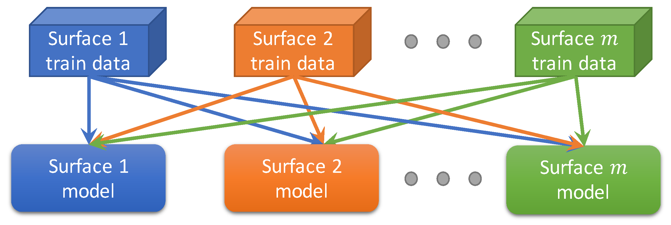
3.3.4. Multi-Task Learning

Multi-task learning (MTL) has emerged as a solution for improving the surface shape modeling by transferring the knowledge among multiple similar-but-not-identical surfaces. Here, one “task” is defined as modeling the surface shape using partial measurement data. Figure 5 illustrates the learning scheme of MTL. It can be particularly useful in a scenario when the amount of available measurement data is limited for the target surface, while measurement data from other related surfaces are readily obtainable. It was originally investigated in the machine learning community [87,88], and has been used successfully in multiple engineering applications. Compared to that each task is learned individually, i.e., single-task learning, MTL has proven to significantly improve the learning performance through jointly learning all tasks [49,89]. In the automotive industry, an engineering-guided MTL approach has been developed to improve the machined surface shape prediction by integrating MTL with cutting force variation modeling [49]. Chen et al. developed a framework to integrate spatiotemporal interpolation methods and MTL for further improving the modeling performance and reducing the measurement cost in data scarce situations [16].

3.4. Interpolation Methods for Discrete Variation

3.4.1. Inference with Discrete Spatial Processes

Most existing methods for constructing probability model over discrete lattices are based on the concept of Markov random field (MRF). In general, MRF is a set of random variables defined regarding an undirected graph, of which each node represents a random variable, and any two non-adjacent variables are conditionally independent given all other variables. MRFs have found wide application for analyzing images, which are 2D lattices of (light intensity) data sampled over uniform grids, suggesting its potential application for surface measurements.
A given lattice may be extended to different graphs by specifying edges connecting its vertices, to describe such probability dependence among its values. When the joint distribution is Gaussian (Gaussian MRF, GMRF [90]), such conditional independence is equivalently characterized by a zero of corresponding entry in the precision matrix (i.e., inverse of the covariance matrix).
In more general cases, an MRF is usually specified by potential functions over cliques of the graph, with the help of the Hammersley-Clifford theorem. Different potential functions yield MRFs with various behaviors, making MRF quite flexible (e.g., Product of Experts model [91,92]).
MRFs could also be defined in terms of conditional autoregressions. When the resulting joint distribution is improper (usually in the context of GMRF), the model could characterize intrinsic autoregressions. A recent paper [93] discussed the relationship between autoregressive GMRF and convolutional neural networks (CNNs) and described extensions of GMRF to higher-order.

3.4.2. Compressed Sensing

Compressed sensing (CS) [94,95] methods exploit the sparsity of signals in certain transform domain. It considers a discrete signal in R N , which after a linear transformation becomes ξ R N with at most K N non-negligible elements. The basic theory [96,97] of CS claims that ξ (equivalently, f) could be efficiently recovered from M O ( K log N ) generally “random-like” linear projections R = A ξ of ξ , where A M × N models the measurement procedure and is called sensing matrix. The proposed reconstruction method, known as the basis pursuit algorithm, recovers ξ by solving min ξ λ ξ 1 s.t. R A ξ 2 < ϵ , which is a convex optimization problem. These fundamental results could be viewed as a concentration property related with the geometry of high-dimensional spaces and random vectors (see the first chapter of [96] and [98] for details).
In the existing literature, CS-related methods are not regarded as interpolation. The theory of CS is generally considered to be parallel to the sampling theory described in Section 3.2.1, and viewed as a branch of the more universal theory about sampling, which studies when and how a signal could be recovered from its measurements. Both the theory of Section 3.2.1 and CS involve two major stages: (1) measure the signal f with instrument, obtaining a set of values O, and (2) recover f with O. Their differences are briefly discussed as follows. In sampling theory, f is continuous and O = { f ( x i ) } consists of values of f over a set X = x i . In stage (1), X is usually specified via distribution pattern and density of its points; e.g., X forms a uniform grid of certain fixed size. In stage (2), the aforementioned interpolation methods are used to reconstruct f.
In CS, f is discrete and rearranged into a vector; O contains linear projections of f, which are generally not values of f. In stage (1), measurements in O are specified by previous A and a sparsifying transform. Then CS reconstruction algorithms are applied in stage (2), serving as interpolation, in the broad sense of estimating function values from relevant information. However, we do not make such separation here, since the coupling of stage (1) and (2) in CS could be strong.
With the sampling theory of Section 3.2.1, one must make sufficiently dense measurements to recover a signal that may change quickly, as suggested by Shannon’s theory. However, it is not always possible and desirable to perform such many measurements required by the theory. CS has then received attention [99] because of its ability to bypass this density limitation, which allows the reconstruction of signals from fewer measurements. Another reason is the wide existence of signal sparsity in transform domains (e.g., Fourier/wavelet domain), which suggests a broad range of potential applications.
The quality of CS reconstruction depends heavily on the properties of the measurement strategy (or sampling design) and the reconstruction algorithm, which are in turn based on different models and structures in specific cases. We note that the relevant developments are very rich in the CS field. For example, (1) characteristics of feasible acquisition hardware and objective signals could be exploited to achieve better applicability and sampling efficiency [100,101]; (2) performance of the reconstruction algorithm could be further improved (sometimes coupled with the sampling design), in terms of computational efficiency and restoration quality [102]; (3) theories could be extended to more general cases [103]; (4) advances in machine learning may be adopted to enhance CS [104]. It is out of the scope of this paper to discuss them in detail.

3.4.3. Image Super-Resolution

Image super-resolution (SR) refers to techniques developed for obtaining high-resolution (HR) images from low-resolution (LR) observations [105]. To distinguish with continuous spatial-only interpolation methods described in Section 3.2, which could also be used for increasing pixel density, SR methods are generally characterized by their ability to restore high-frequency details, which are filtered by linear spatial-only interpolation.
Another relevant concept is optical SR or SR imaging, whose application in surface metrology is reviewed in [106]. Although SR imaging is mainly about overcoming the physical limits (e.g., diffraction) of the optical system, image SR mentioned here is in more about dividing the sensor pixel.
In the context of spatial interpolation, we are more interested in single-image SR (SISR), which makes use of a single low-resolution image, unlike multi-image SR methods. Most image SR methods adopt an imaging model [105] that assumes LR observations are obtained by imaging the same scene with larger sensor pixels. With this model, LR observations are obtained by linear blurring and down-sampling an HR image, and image SR aims to revert this procedure. For SISR, this inverse problem is ill-conditioned. Different methods make use of prior information from various image models to overcome the problem. Refer to [105,107] for relevant reviews.

3.4.4. Comments on Discrete Methods

Essentially, because of the similarity between surfaces and images, most methods described in this subsection, which can deal with images, may potentially be transferred to process surface data. However, we stress that surface measurement is generally different from imaging in mechanism. For example, stylus-based instruments perform highly localized measurements, which do not involve the averaging operation on sensor pixels. This difference should be noted when adapting methods for images to surface data.
Compared to concepts in continuous interpolation, we may notice that most discrete interpolation methods mentioned are “spatial-only”. However, methods developed for videos may be likewise considered for spatiotemporal processes. Instead of Euclidean distances, many discrete methods depend more on some graph structure to characterize correlations, which my lead to more straightforward extensions to account for multivariate cases.

3.5. Surface Interpolation in Manufacturing

The interpolation techniques reviewed in this section are generally applicable for multi-dimensional interpolation. These methods have found various applications in the manufacturing context; however, many of them are less often used to deal with surface measurements. Specifically, sampling theories and CS [108] are more often regarded as methodologies for signal acquisition and processing in general. Methods related with RKHS, curve fitting, GPR, and local regression often serve as standard regression techniques in statistical learning. MRF-based methods and image SR normally deal with images. MRF is often related with pattern recognition tasks, and image SR is rarely used for applications other than image quality/resolution enhancement.
When we restrict the scope to interpolating manufacturing surfaces, the existing literature is concentrated on some of the techniques reviewed. Kriging-type (e.g., [11,109]) and data fusion methods (e.g., [3,12,14,16,49,83,85,110]) are more often used for surface measurements. Cubic B-splines [111,112,113] and convolutions are typically applied for interpolation, when samples are taken over a regular grid. In addition to kriging, fitting with cubic B-spline basis, RBF interpolation, and mesh-based methods are often adopted [76,109,112] for scattered measurements. Generally, smoothing splines (like thin-plate splines) are only used when smoothing is needed [114]. When it is required (e.g., for CAD modeling, reverse engineering) or necessary (e.g., for free-form surfaces) to represent the surface in a parametric form, fitting with B-splines and NURBS [64,115] or constructing meshes [116] are the common practice. Modeling of real 3D surfaces is beyond the scope of this review, despite its wide applications in manufacturing. The possibility of applying CS to surface metrology was explored in [117,118], which still requires implementation with measurement instruments. Currently, only CS-AFM [119] is relatively mature among existing work of relevance.

4. Sampling Design

Sampling design, also known as measurement strategy in some manufacturing applications, represents the distribution of sampling locations. Mathematically, a sampling design can be described by a set of geographical coordinates, e.g., ( x , y ) . For spatiotemporal processes, temporal information is added such that a set of ( x , y , t ) is used to characterize a spatiotemporal sampling design. Sampling design affects the interpolation accuracy and precision greatly, so it should be carefully chosen so that the measurement efforts can be optimally allocated. An optimal sampling design could reduce the measurement cost while maintaining a satisfactory prediction performance. In the literature, sampling points, sites, locations, and units, are used interchangeably to describe the locations where measurement is performed. Although sampling design methods or measurement strategies have received extensive attention across different fields, most studies on sampling design have adopted or extended concepts and techniques stemming from geostatistics [67]. Sampling design for surface measurement in manufacturing was not as extensively studied as in other fields, but it has received increasing attention in the past decade. Example publications include [9,12,32,120]. In the remainder of this section, model-free and model-based sampling design are first summarized, and then different searching algorithms for sampling design are reviewed.

4.1. Model-Free Sampling Design

Model-free sampling is also known as design-based or probability-based sampling. In this approach, samples are selected with an equal or an unequal probability. Such a probability-based paradigm is based on classical sampling theory. Common mode-free sampling methods include random sampling, systematic sampling, stratified sampling, and two-stage sampling [121], the first three of which are illustrated in Figure 6.

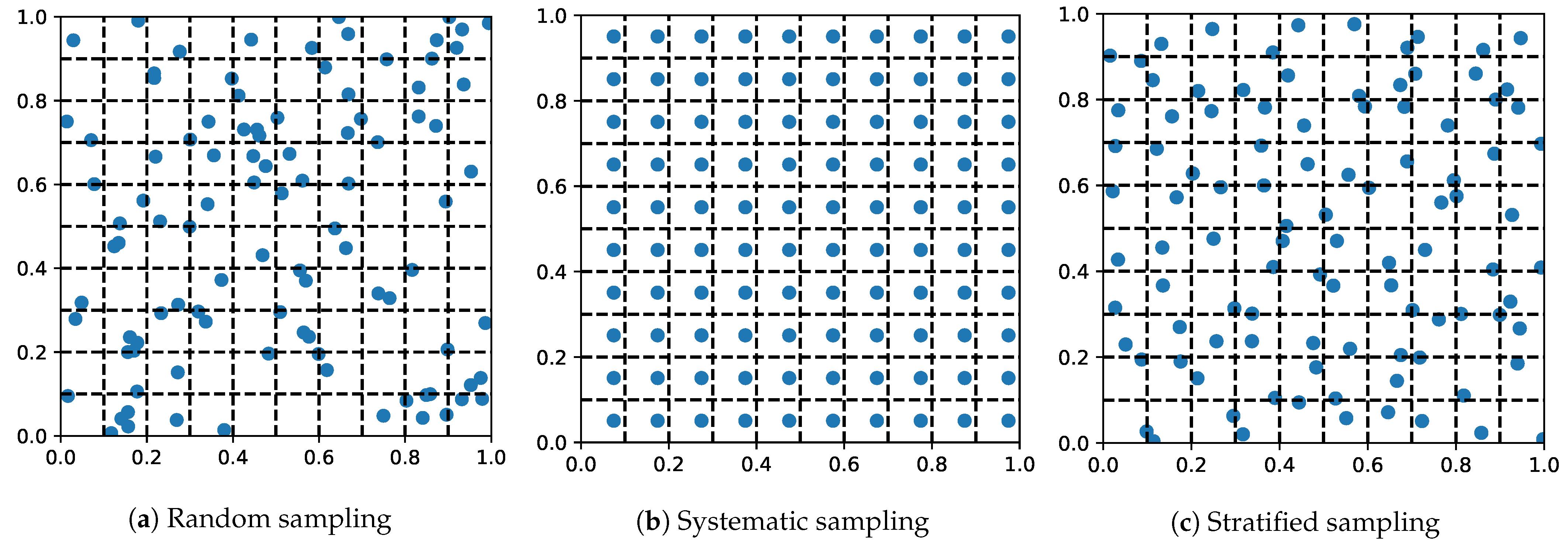
4.1.1. Random Sampling

In random sampling, the values at all locations are assumed to be independent and identically distributed (i.i.d) random variables, and sampled units are drawn from the population independently with equal probability [122,123]. The scheme of random sampling is shown in Figure 6a. As a basic sampling design method, it is convenient to implement and has been widely used in practice. Random sampling is often used as the benchmark method in comparisons with more advanced designs. This sampling approach may not reflect the underlying processes efficiently because it may over-sample some areas while under-sample others.

4.1.2. Systematic Sampling

The population is also assumed to be i.i.d in systematic sampling. Once the first sample unit is randomly drawn from the population, the remaining sampling units are aligned in a given preset order relative to this first point [122]. The scheme of systematic sampling is shown in Figure 6b. Systematic sampling is also referred to as uniform sampling or regular sampling when the first sample unit is not chosen at random. With systematic sampling, the observations are spread evenly across the space domain. The spreading of the observations prevents sampling from clustering and guarantees a representative coverage.

4.1.3. Stratified Sampling

In stratified sampling, the population is assumed to be spatially stratified. The population is divided into non-overlapping sub-populations called strata, and samples within each stratum is assumed to be i.i.d. [67]. Figure 6c shows an example of a stratified sampling design, where the whole space is divided into 100 squares of equal size and one unit is randomly selected from each stratum.

4.1.4. Two-Stage Sampling

In two-stage sampling, the population is also divided into non-overlapping sub-populations, while not all sub-populations would be sampled. The first stage in two-stage sampling samples the sub-populations, and then the units in the selected sub-populations are sampled. At each stage, different sampling approaches can be used. The two-stage sampling approach can be extended to multi-stage sampling [67].

4.2. Model-Based Sampling Design

Although most model-free sampling methods are convenient to implement in practice, the spatial information in the region of interest is neither modeled nor used, and this often leads to a non-optimal design and/or high measurement cost [121]. Model-based sampling design methods aim to overcome such drawbacks by using the spatial/spatiotemporal information in the design process. In the model-based sampling design, a collection of statistical methods originated from geostatistics can be used to describe the spatial autocorrelation among sampling locations. Additionally, a model-based sampling design can use the spatial information to formulate a predefined objective function as the design criterion, and find a set of observed locations such that the inference at unobserved locations is optimized according to the design criterion.
In most manufacturing applications, the sampling locations and observation times are assumed to be discrete in finite spatial and time domains, respectively. In this section, we will focus on sampling design problems in spatial domain, and spatiotemporal sampling design will be discussed in Section 4.3. A spatial sampling design problem can be generally formulated as follows. We denote the location set of interest by S . In spatial sampling design problem, S can be represented by S = { s 1 , , s n s } D s , where D s is the spatial domain and n s is the total number of spatial locations. S is divided into two sets: the set of observed points S o S , and the set of unobserved points S u = S \ S o . The goal of sampling design is to select an optimal S o regrading the design criterion.
The performance of a sampling design is the most important component in the design criterion. A common performance measure of a sampling design is the prediction error variance, which can be estimated through interpolation techniques that can quantify the prediction uncertainty at a particular location, such as kriging, GP model, and state-space model. The objective function can be formulated as a function of the prediction error variances at unsampled locations, and the sampling sites should be optimally allocated to minimize the prediction error variances [9,12,32,120]. Distance-based criterion is another popular choice for the performance measure of a sampling design. It aims to have sampling locations well-spread over the surface of interest. The objective function can be formulated as a function of the shortest distances from unsampled locations to the nearest sampled locations [121,124].
Measurement cost should be jointly considered in the sampling design criterion when online monitoring is not feasible. In most cases, the major source for the measurement cost is the measurement time, which is proportional to the total number of measured points. The cost of measurement time could depend on the measurement system available. As mentioned in Section 2.1, optical measurement systems can measure a part of surface with one-time scanning, and there is a trade-off between the measurement range and resolution. Measurement with higher resolution generally would cover a smaller range, and the relative measurement cost for each measured point would be higher. There are two ways to put the measurement cost into the design criterion. First, the measurement cost can serve as a constraint for the design criterion. For example, the number of sampled sites can be required to be smaller than or equal to a predefined threshold [32,84,120]. The performance of different sampling designs can be compared under the same measurement cost constraint. With the constraint approach, the sampling design may tend to measure as many locations as possible, because in general a better sampling performance can be achieved with more sampled locations. Another choice is adding the measurement cost into the design criterion directly. Because the measurement cost and the design performance are different quantities, weighting coefficients can be used to represent the relationship between these two quantities. This approach provides a flexibility to make a trade-off between the cost and performance. However, weighting coefficients may need to be chosen carefully with expert knowledge [9,12].
The sampling design problem can be formulated as a binary integer programming problem. A straightforward solution to the sampling design problem is to exhaustively calculate the criterion value for all potential sampling designs. However, such a NP-hard problem cannot be solved in a polynomial time, and this approach is feasible only when the search space is small, which is not a common scenario in manufacturing applications. Assume there are N x × N y observable locations on the surface. For each location, there are two decisions we can make: measure it or skip the measurement. The number of all possible designs increases exponentially with the number of locations. Taking a 10 × 10 surface as an example, i.e., N x = N y = 10 , the number of all possible designs is 2 10 × 10 1.27 × 10 30 . In practice, the dimension of the solution space could be much higher. Hence, searching algorithm is necessary for finding the optimal solution in a computationally efficient manner. Various optimization algorithms have been adopted for searching optimal sampling design in the literature. Here, we will discuss two representative techniques for surface metrology applications in manufacturing: adaptive sampling algorithm and heuristic sampling algorithm.

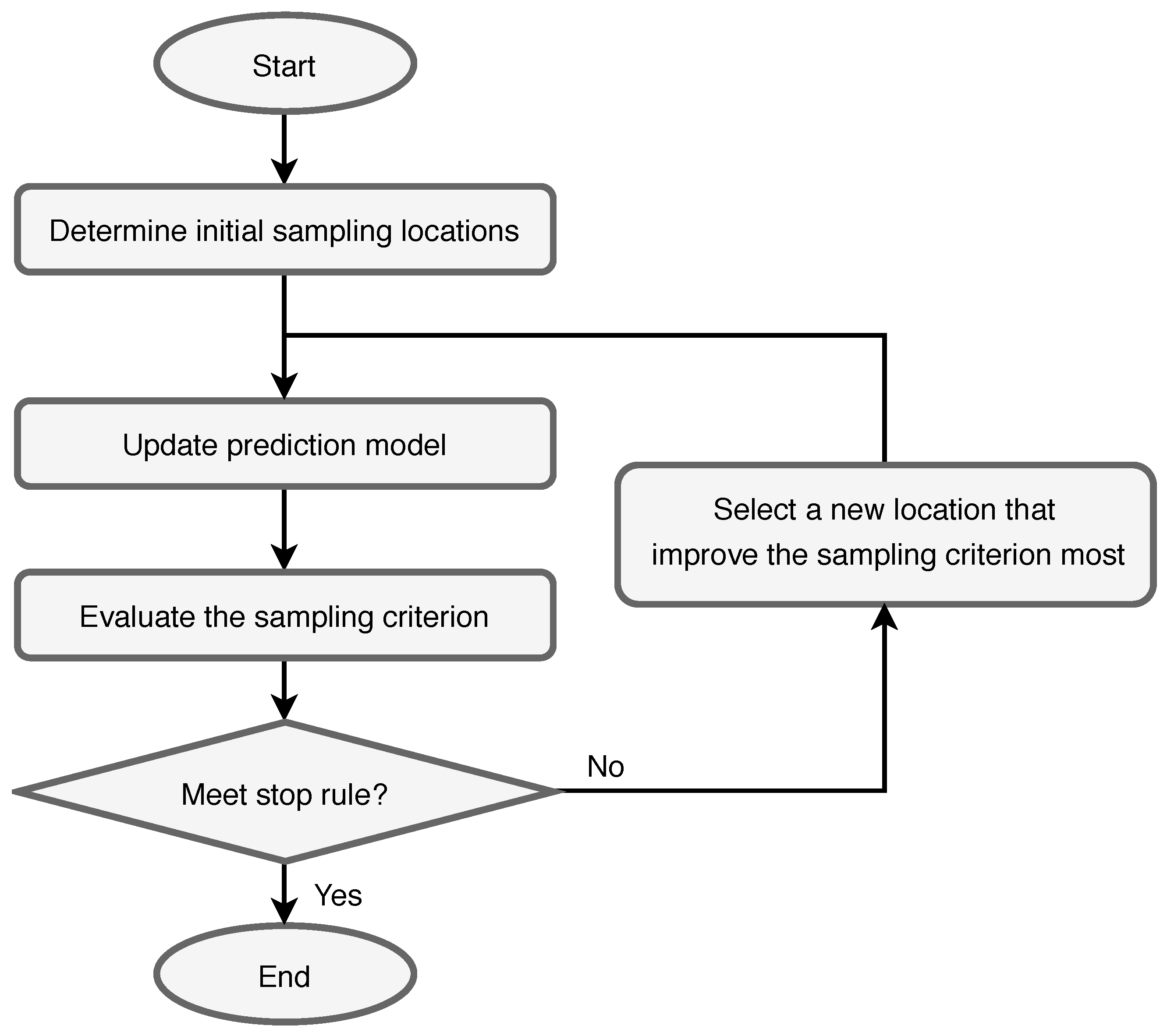
4.2.1. Adaptive Sampling

In the adaptive sampling, the sampling locations are allocated sequentially based on prior information. It is also known as sequential sampling or progressive sampling. Figure 7 shows a typical procedure of adaptive sampling design. In the initialization of adaptive search, a small set of locations are selected as initial sampling locations which can be determined using prior engineering knowledge or model-free sampling. After the initial sampling locations are determined, a prediction model is trained based on them, and the design performance is subsequently evaluated. The location that can improve the objective function most is selected as the next sampling location in the following iteration. In each iteration, the prediction model is updated with all sampled locations, and a new location is selected for next iteration. After each iteration, the stopping rule is checked, and the iterative measurement procedure stops if it is satisfied.
A recent investigation of adaptive sampling design in manufacturing has been reported by Jin et al., where a systematic measurement strategy is developed for wafer surface quality monitoring and the sequential design approach is combined with prior engineering understanding of the wafer cutting process [32]. Lalehpour et al. also employed the adaptive sampling approach to effectively inspect various distributions of geometric deviation in manufactured surfaces with a small number of sample points [120]. However, for a problem with many sampling locations, the number of iterations can also be large with the adaptive or sequential sampling algorithm, and the implementation of such approaches can be very computationally expensive. It might be challenging to improve the computing efficiency because the new sampling location are added incrementally.

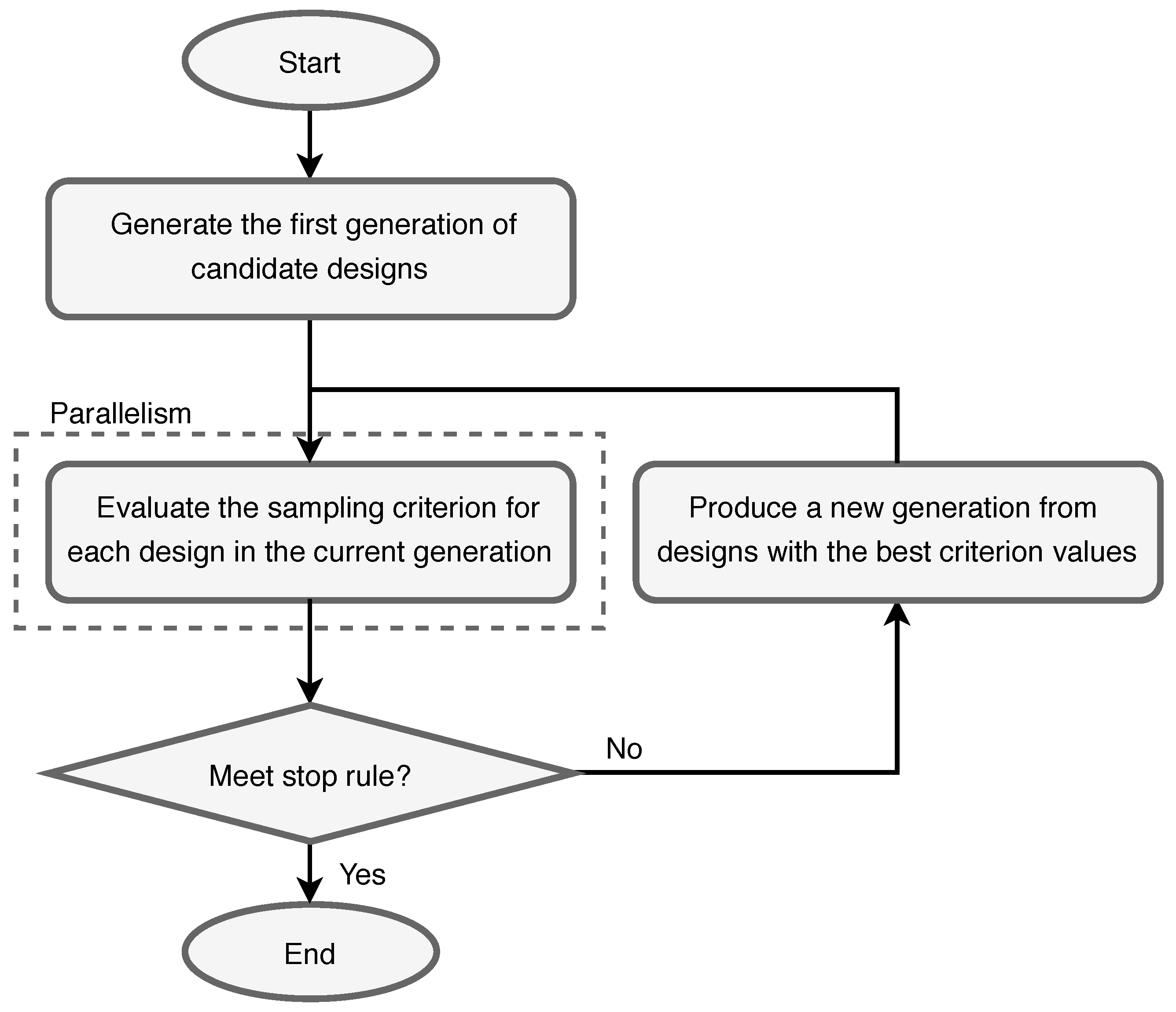
4.2.2. Heuristic Sampling

Heuristic search algorithms have been proven to be effective in dealing with binary integer programming problem with high-dimensional solution space. Several heuristic algorithms, including simulated annealing, particle swarm optimization, and genetic algorithm (GA), have been adopted in the existing literature [9,12,125]. Without loss of generality, GA is reviewed in this section. Figure 8 shows the procedure of GA for sampling design. The idea of GA is inspired by the process of natural selection, recombination, and evolution. In the initialization of GA, the population of candidate sampling designs, called the first generation, is generated randomly from all possible designs. Then a prediction model is trained for each candidate design and the corresponding design criterion is evaluated. After the evaluation, the “elitists” in the current generation, which are the sampling designs with the best criterion values, are selected, and a new generation of sampling designs is produced by recombination and mutation of the selected elitists. The process of selection and reproduction is repeated for every successive generation until a stop rule has been satisfied. Most heuristic algorithm-based sampling methods have a similar implementation, i.e., a set of candidate solutions are maintained and improved over iterations, and the key difference between them is the way of updating the candidate solutions.
In general, for sampling design problems with a high-dimensional solution space, it is required to have many candidate sampling designs at each generation and many iterations so that the heuristic algorithms can converge to an optimal solution [12]. However, the execution time of such a computationally intensive application can be extremely long with sequential computing. Leveraging a large amount of computational power from a cloud-based environment or high-performance computing (HPC) with parallel computing can significantly improve the computational efficiency of big data analytics [12,126]. A generic framework with an implementation procedure and a series of guidelines for heuristic sampling design in HPC environments can be found in [126].

4.3. Spatiotemporal Sampling

In spatial sampling design problems, only the numbers of and spatial distributions of sampling locations are considered. All measurements are assumed to be made at a given observation time. In real-world manufacturing, manufacturers may want to know when they should make observations first, and where the measurement efforts should be allocated at a given observation time. The location set of interest in a spatiotemporal process can be denoted by S = { ( s 1 ; t 1 ) , , ( s n s ; t 1 ) , ( s 1 ; t 2 ) , , ( s n s ; t n t ) } D s × D t , where n t is the total number of observation times and D t = { t 1 , t 2 , , t n t } is the temporal domain. Figure 9 provides one example scheme of the spatiotemporal sampling design. Each blue grid represents one scan in an optical measurement system. The points covered by blue grids are belong to S o . In spatiotemporal sampling design, the number of observation time is another major source of the measurement cost, because each observation will lead to a fixed large amount of production downtime as long as some points need to be measured at that time. As shown in the example in Figure 9, no point needs to be measured at time 4, and the observation at time 4 can be skipped and the total measurement cost can be reduced significantly. It is desirable to skip some observation time for reducing the measurement cost while maintaining a satisfactory modeling performance in spatiotemporal sampling design.
Spatiotemporal sampling design approaches can be divided into two main categories: static sampling design and dynamic sampling design, depending on how the dependence in the temporal domain is treated. In static sampling design, the temporal dependence of spatial structure is assumed to be negligible and the spatial structures at different time points are homogeneous. In this case, the time domain is treated a completely separate dimension, and the spatial sampling design techniques can be adopted as static sampling design.
However, when the space-time interactions exist in the spatiotemporal processes, as in many manufacturing applications (e.g., [9,12,84]), the spatial structure varies over time. In such cases, leveraging the temporal correlation may further reduce the requirement on data availability. Static sampling design methods are not applicable in these scenarios. Dynamic sampling design methods are desired to characterize the time-variant spatial structure pattern. Both adaptive approaches and heuristic approaches described in Section 4.2.1 and Section 4.2.2 can be extended for dynamic spatiotemporal sampling design, as explained below.
Extending adaptive sampling approach from spatial sampling to spatiotemporal sampling is relatively straightforward. First, a spatiotemporal prediction model should be used to modeling the time-variant spatial structure pattern. Second, the new sampling location selection at each iteration needs to be based on all sampled locations at the current and prior time stages. For example, Babu et al. used a state-space function to model the spatiotemporal surface deviations of parts in an automotive machining process and adopted spatiotemporal adaptive sampling for measurement region selection [84]. Specifically, the whole surface is divided into 9 regions. The sampling regions at each observation time is selected one by one as described in Section 4.2.1, and the process is repeated for observation times staring from the first observation. Although this extension of adaptive sampling is easy to be implemented, it faces the same challenges in computing efficiency when the sampling design problem comes with many sampling locations.
To improve the computation efficiency for spatiotemporal sampling design problem with many spatial locations, Shao et al. adopted heuristic sampling in their dynamic sampling design approach for spatiotemporal processes [9]. GA is used for solution search in the optimal spatial sampling design at each observation time. In addition, spatiotemporal state-space function is adopted, and a hypothesis testing is developed for monitoring and updating the temporal transition parameter of the surface progression. In other words, heuristic sampling is used to determine the sampling locations in spatial domain and no observation times is skipped.
These two dynamic sampling design approaches could be considered to be sub-optimal because measurement could be made at all observation times. Conventional heuristic algorithms may not be applied directly for the spatiotemporal sampling design, because they can be easily stuck at local optimal solutions. Hence, customized implementation of the conventional heuristic algorithms is required for preventing premature convergence. In general, decisions need to be made at more locations in spatiotemporal processes than in spatial processes, larger amount of computing resources is required to enable responsive decision-making. Yang et al. formulated the spatiotemporal sampling design as a two-level decision-making problem, and adopted hierarchical GA to search the optimal sampling design efficiently [12]. With the hierarchically structured representation of sampling design, the number and distribution of the observations time are determined first, and then the measurement efforts at each time are allocated. In other words, the decision of allocating measurement efforts is made hierarchically. Multi-node parallelization on HPC is employed for sampling design in a real-world ultrasonic metal welding process. They reduced the average running time of the heuristic search algorithm by hundreds of times and enabled responsive sampling design with high-dimensional solution space.

5. Future Work

5.1. Performance Evaluation of Interpolation Methods

In existing studies, the evaluation of interpolation performance is rather simple. Prediction errors such as RMSE, MAE, and mean absolute error percentage are popular choices. Such performance metrics are straightforward to use and provide a clear evaluation of the interpolation performance. Nevertheless, the applicability of interpolation methods should be more carefully justified when the interpolated results are used as inputs to the downstream decision-making process, e.g., quality monitoring, process control, maintenance in manufacturing. Usually guided by minimizing the prediction errors or uncertainties, the interpolation process does not try to preserve other properties of the true spatial/spatiotemporal process, which may be used by the decision-making algorithm. In situations where a low prediction error would be sufficient, interpolated results are directly applicable; but it is not always the case.
Such phenomenon is the most obvious for spatial-only continuous interpolation when compared in the frequency domain. For example, linear methods of this type have a low-pass filtering effect. Thus, the discrepancy between f ^ and f is usually negligible in the low-frequency range, but becomes large for higher frequencies, eventually leading to significant relative errors at the high-end of the spectral. This means fine features below certain scale cannot be preserved by linear interpolation methods, suggesting their incapability in many cases. For instance, when interpolated data are used to calculate power spectral density of surface topography, the result would not be reliable at the high-frequency end. Consequently, non-optimal or even poor decisions may be made if the decision-making process uses the high-frequency information.
The loss of high-frequency information may be eased by more-than-spatial methods that involve other signals, or by discrete compressive methods that use prior knowledge of f. In both cases, the extra information required is relevant to finer scale details. These methods may be practically useful, but it is challenging at the moment to theoretically characterize the introduced uncertainties.
Error propagation is another important issue to investigate such that a better understanding of how the interpolation performance (in terms of both precision and accuracy) influences the downstream decision-making performance. In many cases, it may be very challenging to obtain analytical solutions. One possible direction is to use sensitivity analysis and computational algorithms, e.g., Monte Carlo experiments.
On a relevant note, the connection between the interpolation and the subsequent decision-making should be systematically studied such that the best interpolation techniques can be selected. We illustrate this point with a few examples. For visual inspection, monitoring or numerical quadrature, we often hope to preserve details, and point-referenced results with smaller prediction errors, e.g., in terms of RMSE, may be satisfying. To build CAD models from measurements, when larger-scale features such as size are more important, methods producing concise representation would be preferred. In some other applications, including defect detection, where interpolation could be used as data enhancement, it may not be necessary because information introduced to assist interpolation may be directly incorporated in relevant task-specific algorithms.

5.2. Big Data Fusion for Interpolation

We envision that it is worth devoting future research efforts to the development of more powerful data fusion approaches. The rapid development of sensing and communication technologies as well as manufacturing cyberinfrastructure has made it possible to collect and use a large volume of data from different sources at a much lower cost. Yet, the potential of data fusion has not been fully exploited in general and in surface data interpolation. Data sources that can be fused in interpolation include the surface itself, the measurement mechanism, the manufacturing process involving the surface of interest, related manufacturing processes and systems, maintenance procedure in production, and the measurement instrument used. Similar ideas have been explored in [127], where such integration is termed as “information-rich metrology.” Here, we attempt to relate it to interpolation techniques in manufacturing surface measurement. We first consider a rather high-level and abstract description of the entire (but static) process, to get a better understanding of our position. Denote the quantity of primary interest as f : R 2 R , e.g., the surface topography; denote the distribution of other quantities as g, e.g., material composition, or other relevant mechanical/electromagnetic properties, which may also affect the surface-instrument interaction. Once the sampling scheme S is determined, the instrument could be abstracted as an operator L S , γ with measurement errors, where γ captures factors including instrument parameters and environments. The surface and instrument interact with each other and produce raw data R = L S , γ ( f , g ) . Then, an operator I ˜ S , γ , representing some data processing procedure, acts on R = L S , γ ( f , g ) and yields y = I ˜ S , γ ( R ) R M . Often y is supposed to approximate the value of f at a set of locations X, i.e., y f ( X ) . With a continuous interpolation method denoted as an operator I n t X , data is converted back to a mapping f ^ = I n t X ( y ) over a continuous region, such that f ^ f . This process is shown by Equation (6).
( f , g ) L S , γ ( f , g ) = R I ˜ S , γ ( R ) = y f ( X ) I n t X ( y ) = f ^ f .
All involved computational procedures I ˜ S , γ I n t X , are essentially about inverting approximately the measurement mechanism L S , γ . Interpolation methods for continuous variation deal with I n t X . Discrete interpolation methods are a bit different. Image SR may be viewed as a layer that enhances any lattice data to finer grids, as long as there is knowledge about correspondence between data of different resolution; thus it may be inserted into I ˜ S , γ as a stage after data from camera-like sensors, or put between I ˜ S , γ and I n t X merely as a soft enhancement for I n t X . CS methods are more closely related to the measurement procedure. True CS implemented with hardware requires linear measurements that satisfy certain properties, which are captured by S and L S , γ . The reconstruction method for such schemes is integrated into I ˜ S , γ . At the same time, CS reconstruction could also be put before I n t X such as image SR. In this case, the linear measurements are determined by X (which may not be necessarily the same as S).
We may see that with prior information about f, the only thing we can do, after data has passed through I ˜ S , γ resulting in y, is to select proper I n t X among continuous interpolation, and perhaps enhance it with discrete methods. It is obvious that such improvement at the final stage is always and essentially limited by the quality of y. One approach to ease this limitation is to get more information about f from other sources, as in data fusion-based interpolation methods. Without dealing with I ˜ S , γ , another improvement may be made by studying the statistical properties of error y f ( X ) ; depending on the measurement mechanism and the internal data processing procedure, behavior of the error could vary substantially.
Other improvements can be achieved by modifying I ˜ S , γ . This could be viewed in the general context of inverse problems, where we use I ˜ S , γ to approximate L S , γ 1 . There are several challenges associated with this inversion. First, it is impossible in principle to express the inverse L S , γ 1 in terms of f only without knowing g; the best one could get is an approximation that works for most g, which always comes with error. Second, approximation may be made in inverting the mechanism L S , γ because of various difficulties, which also lead to prediction errors. For example, the model L S , γ could be incomplete if not all factors are considered; or simplifications must be made for computational tractability. Third, most inverse problems involve ambiguity, and assumptions must be made so that the problem becomes well-posed. Without more information about ( f , g ) , in general these assumptions are weak, and the inversion I ˜ S , γ could lead to poor results. (Here we use ( f , g ) to emphasize that f and g together, instead of f alone, form the complete set of factors from the surface that affect the measurement process.)
From discussions above, we could see that knowledge about f and relevant g must be incorporated into the inversion procedure for further improvements. We suggest a few possible future research directions.
(1)
The aforementioned true CS measurements can be implemented with hardware. Prior knowledge about f (e.g., its transform-sparsity) and the mechanism of the instrument need to be integrated, to design proper measurement strategy and reconstruction algorithm. Image SR could also be used to enhance camera-like sensors. Please note that CS reconstruction and image SR are both examples of (mostly linear) inverse problems.
(2)
Knowledge of ( f , g ) can help reduce the ambiguity of the relevant inverse problem. Also, theory of statistical inverse problem may be adopted [128]. It represents prior knowledge about f in terms of a prior distribution, and the inverse problem naturally converts to Bayesian inference, for which the ambiguity could be quantified as variance of the posterior distribution.
(3)
Knowledge of ( f , g ) can help build models for L S , γ in the “operation range” (around ( f , g ) ), so that it is more precise, less ambiguous, and computationally simpler to invert.

5.3. Advanced Sampling Design

As discussed in Section 4, most existing model-based sampling design methods basically aim to optimize a predefined design criterion, which can be the prediction variance or a weighted sum of the prediction variance and measurement cost. The existing problem formulations have the following limitations.
First, the prediction variance may be very challenging to obtain in some interpolation/prediction methods. In the existing research on sampling design, kriging and GP models, and their variants are commonly used for interpolation and the estimation of prediction variances. The accessibility of prediction variances in these methods comes from the underlying assumption on statistical distributions, which are often Gaussian. However, for some other methods, the prediction variance estimation can be very difficult due to different data distribution assumptions. Sampling design methods for these interpolation techniques are needed.
Second, the existing sampling design methods often focus on one target variable (e.g., surface height) but fail to specifically account for other spatial features (e.g., flatness and surface roughness in machining processes, tool degradation level in ultrasonic welding). In some applications, an accurate estimation of these features is probably more important than accurately estimating every location on the surface. New problem formulations should be devised accordingly.
Third, improved problem formulations that can better take measurement cost into consideration are necessary. As previously discussed, measurement cost is typically considered through either adding a penalty term to the design criterion or posing a constraint to the solution space. Yet, the link to the physical measurement process is not sufficiently accounted for and the estimation of measurement cost is very simplified, e.g., as the total number of measured locations. In real-world manufacturing applications, measurement cost may manifest itself in multiple ways, e.g., the cost of the measurement system including both the capital and consumable costs, the measurement time induced by moving the part to the metrology fixture, warm-up and calibration of the measurement system, and the actual measurement time.

5.4. Instrument Automation

As summarized in Section 4, the methodology development of sampling design has been actively discussed across different fields. However, as a matter of fact, the sampling design or measurement strategy has not been integrated with the measurement instruments that are commercially available. Most existing studies in manufacturing are based on computational simulation or customized implementation. Some recently developed surface measurement instruments support an automated scanning mode, i.e., the scans are repeated until the whole region of interest is covered, and some post-measurement data processing functions, e.g., stitching multiple measurement regions into a larger one, data cleaning and de-noising. Nevertheless, most existing measurement instruments do not allow two-way communications with sampling design algorithms or flexible measurement path planning. This limitation in hardware implementation has become a major hurdle for the application of sampling design methods in the real-world settings, especially in the manufacturing industry where the production volume is high and a strong demand for responsive decision-making exists.
We envision that a higher-level instrument automation is an imperative in the next-generation high-resolution 3D surface measurement systems. The development of such systems calls for collective efforts from the manufacturers and end-users of metrology equipment, software engineers, as well as researchers that work on the development of sampling design algorithms.

5.5. MSA of High-Dimensional Surface Data

As reviewed in Section 2.2, existing MSA methods for surface measurement data rely upon the classical MSA framework, the overarching assumption of which is that the variable(s) of interest, which can be extracted features or original measurements, is normally distributed. Under this assumption, ANOVA and MANOVA work well with single-dimensional and low-dimensional data. When the original measurement data is high-dimensional, one must apply dimensionality reduction to be able to use ANOVA/MANOVA. Yet, such a feature extraction process breaks the original data structure and therefore cannot account for the inherent data correlations, e.g., spatial correlations. In addition, information may be lost in the process of feature extraction and location-wise capability assessment is therefore not available. One possible solution is to conduct pointwise MSA to all locations on the surface, but it fails to capture the spatial correlations (similarities or differences) among different locations.
It is more challenging to conduct MSA for interpolated surface data. As mentioned earlier, interpolation is a necessary part of the data registration process; and it is an enabling technique for cost-effective surface measurement. However, the interpolation process is never perfectly accurate, thus introducing additional errors and uncertainties to the interpolated data. As such, the resulting variation in the interpolated data is caused by both the measurement process and the interpolation process. Furthermore, since interpolations make use of the measurement data at other locations, there exists a hierarchical effect with measurement and interpolation at the lower and higher levels, respectively. Under such circumstances, extending the existing MSA methods is non-trivial and more advanced analytics tools are needed.

6. Conclusions

Data analytics plays a pivotal role in the smart manufacturing transformation. Today’s manufacturing industry is using data extensively for decision-making. Among different types of data, surface measurement data are being increasingly collected and analyzed at the levels of manufacturing machines, processes, and systems for intelligent product quality evaluation, machine maintenance, process control, etc. Although the recent advancement in measurement technologies has made it possible to collect high-resolution surface data, the data acquisition is often cost-prohibitive and time-consuming, thereby impairing the agility and cost-effectiveness of smart decision-making in manufacturing. Hence, intelligent surface measurement is critically needed to overcome such challenges. Initially investigated in non-manufacturing areas, data-driven spatial/spatiotemporal interpolation and sampling design are powerful tools that can facilitate intelligent 3D surface measurement in manufacturing. With a focus on industrial applications, this paper reviews the state-of-the-art research in these two fields.
The theoretical and practical contributions of this study are two-fold. First, fundamental theories and applicability of existing methods are summarized, discussed, and compared. Rather than discussing these methods from a solely methodological perspective, we aim to link academic research with industrial practice by paying special attention to how each method can be applied in the manufacturing context. We anticipate that the review will be able to help industry practitioners select the measurement technology and data-driven methods that are most suitable for their production. Additionally, we summarize the most critical challenges that need future research, in both hardware implementation and algorithmic development. It is concluded that collective efforts from both academia and industry will be key to the successful development and industrial implementation of data-driven interpolation and sampling design technologies in the era of smart manufacturing.

Author Contributions

Conceptualization, Y.Y., Z.D., Y.M. and C.S.; methodology and formal analysis, Y.Y. and Z.D.; writing—original draft preparation, Y.Y., Z.D., Y.M. and C.S.; writing—review and editing, Y.M. and C.S.; supervision, project administration, and funding acquisition, C.S. All authors have read and agreed to the published version of the manuscript.

Funding

This research has been supported by the National Science Foundation under Grant No. 1944345.

Institutional Review Board Statement

Not applicable.

Informed Consent Statement

Not applicable.

Data Availability Statement

Not applicable.

Conflicts of Interest

The authors declare no conflict of interest.

Abbreviations

The following abbreviations are used in this manuscript:
AFMAtomic force microscopy
ANOVAAnalysis of variance
BLUPBest linear unbiased prediction
CLMConfocal laser microscopy
CMMCoordinate measuring machines
CNNConvolutional neural network
CSCompressed sensing
GAGenetic algorithm
GLMGeneralized linear model
GMRFGaussian Markov random field
GPGaussian process
GPRGaussian process regression
HPCHigh-performance computing
HRHigh-resolution
i.i.dindependent and identically distributed
KEDKriging with external drift
LHILaser holographic interferometer
LRLow-resolution
LSLeast squares
MAEMean absolute error
MANOVAMultivariate analysis of variance
MRFMarkov random field
MSAMeasurement system analysis
MSEMean squared error
MTLMulti-task learning
NURBSNon-uniform rational B-spline
PTRPrecision/Tolerance ratio
R&RRepeatability and reproducibility
RBFRadial basis function
RKHSReproducing kernel Hilbert space
RMSERoot mean square error
SISRSingle-image super-resolution
SLSStructured light scanner
SRSuper-resolution

References

  1. Nguyen, H.T.; Wang, H.; Hu, S.J. Characterization of cutting force induced surface shape variation in face milling using high-definition metrology. J. Manuf. Sci. Eng. 2013, 135, 041014. [Google Scholar] [CrossRef]
  2. Nguyen, H.T.; Wang, H.; Tai, B.L.; Ren, J.; Jack Hu, S.; Shih, A. High-definition metrology enabled surface variation control by cutting load balancing. J. Manuf. Sci. Eng. 2016, 138. [Google Scholar] [CrossRef]
  3. Suriano, S.; Wang, H.; Shao, C.; Hu, S.J.; Sekhar, P. Progressive measurement and monitoring for multi-resolution data in surface manufacturing considering spatial and cross correlations. IIE Trans. 2015, 47, 1033–1052. [Google Scholar] [CrossRef]
  4. Uhlmann, E.; Hoyer, A. Surface Finishing of Zirconium Dioxide with Abrasive Brushing Tools. Machines 2020, 8, 89. [Google Scholar] [CrossRef]
  5. Grimm, T.; Wiora, G.; Witt, G. Characterization of typical surface effects in additive manufacturing with confocal microscopy. Surf. Topogr. Metrol. Prop. 2015, 3, 014001. [Google Scholar] [CrossRef]
  6. McGregor, D.J.; Tawfick, S.; King, W.P. Automated metrology and geometric analysis of additively manufactured lattice structures. Addit. Manuf. 2019, 28, 535–545. [Google Scholar] [CrossRef]
  7. Townsend, A.; Senin, N.; Blunt, L.; Leach, R.; Taylor, J. Surface texture metrology for metal additive manufacturing: A review. Precis. Eng. 2016, 46, 34–47. [Google Scholar] [CrossRef] [Green Version]
  8. Piotrowski, N. Tool Wear Prediction in Single-Sided Lapping Process. Machines 2020, 8, 59. [Google Scholar] [CrossRef]
  9. Shao, C.; Jin, J.J.; Jack Hu, S. Dynamic sampling design for characterizing spatiotemporal processes in manufacturing. J. Manuf. Sci. Eng. 2017, 139, 101002. [Google Scholar] [CrossRef]
  10. Zerehsaz, Y.; Shao, C.; Jin, J. Tool wear monitoring in ultrasonic welding using high-order decomposition. J. Intell. Manuf. 2019, 30, 657–669. [Google Scholar] [CrossRef]
  11. Yang, Y.; Shao, C. Spatial interpolation for periodic surfaces in manufacturing using a Bessel additive variogram model. J. Manuf. Sci. Eng. 2018, 140, 061001. [Google Scholar] [CrossRef] [Green Version]
  12. Yang, Y.; Zhang, Y.; Cai, Y.D.; Lu, Q.; Koric, S.; Shao, C. Hierarchical measurement strategy for cost-effective interpolation of spatiotemporal data in manufacturing. J. Manuf. Syst. 2019, 53, 159–168. [Google Scholar] [CrossRef]
  13. Suriano, S.; Wang, H.; Hu, S.J. Sequential monitoring of surface spatial variation in automotive machining processes based on high definition metrology. J. Manuf. Syst. 2012, 31, 8–14. [Google Scholar] [CrossRef]
  14. Shao, C.; Wang, H.; Suriano-Puchala, S.; Hu, S.J. Engineering fusion spatial modeling to enable areal measurement system analysis for optical surface metrology. Measurement 2019, 136, 163–172. [Google Scholar] [CrossRef]
  15. Shao, C.; Hyung Kim, T.; Jack Hu, S.; Abell, J.A.; Patrick Spicer, J. Tool wear monitoring for ultrasonic metal welding of lithium-ion batteries. J. Manuf. Sci. Eng. 2016, 138, 051005. [Google Scholar] [CrossRef]
  16. Chen, H.; Yang, Y.; Shao, C. Multi-Task Learning for Data-Efficient Spatiotemporal Modeling of Tool Surface Progression in Ultrasonic Metal Welding. J. Manuf. Syst. 2021, 58, 306–315. [Google Scholar] [CrossRef]
  17. Fortin, M.J.; Drapeau, P.; Legendre, P. Spatial autocorrelation and sampling design in plant ecology. In Progress in Theoretical Vegetation Science; Springer: Berlin/Heidelberg, Germany, 1990; pp. 209–222. [Google Scholar]
  18. Andrew, N.; Mapstone, B. Sampling and the description of spatial pattern in marine ecology. Oceanogr. Mar. Biol. 1987, 25, 39–90. [Google Scholar]
  19. Brown, P.J.; Le, N.D.; Zidek, J.V. Multivariate spatial interpolation and exposure to air pollutants. Can. J. Stat. 1994, 22, 489–509. [Google Scholar] [CrossRef]
  20. White, D.; Kimerling, J.A.; Overton, S.W. Cartographic and geometric components of a global sampling design for environmental monitoring. Cartogr. Geogr. Inf. Syst. 1992, 19, 5–22. [Google Scholar] [CrossRef]
  21. Cressie, N. The origins of kriging. Math. Geol. 1990, 22, 239–252. [Google Scholar] [CrossRef]
  22. David, C.; Sagris, D.; Stergianni, E.; Tsiafis, C.; Tsiafis, I. Experimental Analysis of the Effect of Vibration Phenomena on Workpiece Topomorphy Due to Cutter Runout in End-Milling Process. Machines 2018, 6, 27. [Google Scholar] [CrossRef] [Green Version]
  23. Dzierwa, A.; Markopoulos, A. Influence of Ball-Burnishing Process on Surface Topography Parameters and Tribological Properties of Hardened Steel. Machines 2019, 7, 11. [Google Scholar] [CrossRef] [Green Version]
  24. Durakbasa, M.; Osanna, P.; Demircioglu, P. The factors affecting surface roughness measurements of the machined flat and spherical surface structures—The geometry and the precision of the surface. Measurement 2011, 44, 1986–1999. [Google Scholar] [CrossRef]
  25. Yang, Y.; Chen, S.; Wang, L.; He, J.; Wang, S.M.; Sun, L.; Shao, C. Influence of Coating Spray on Surface Measurement Using 3D Optical Scanning Systems. In Proceedings of the International Manufacturing Science and Engineering Conference, Erie, PA, USA, 10–14 June 2019; Volume 58745, p. V001T02A009. [Google Scholar]
  26. Küng, A.; Meli, F.; Thalmann, R. Ultraprecision micro-CMM using a low force 3D touch probe. Meas. Sci. Technol. 2007, 18, 319. [Google Scholar] [CrossRef]
  27. Bernal, C.; de Agustina, B.; Marín, M.M.; Camacho, A.M. Accuracy analysis of fridge projection systems based on blue light technology. Key Eng. Mater. 2014, 615, 9–14. [Google Scholar] [CrossRef]
  28. Palousek, D.; Omasta, M.; Koutny, D.; Bednar, J.; Koutecky, T.; Dokoupil, F. Effect of matte coating on 3D optical measurement accuracy. Opt. Mater. 2015, 40, 1–9. [Google Scholar] [CrossRef]
  29. Dury, M.R.; Woodward, S.D.; Brown, B.; McCarthy, M.B. Surface finish and 3D optical scanner measurement performance for precision engineering. In Proceedings of the 30th Annual Meeting of the American Society for Precision Engineering, Austin, TX, USA, 1–6 November 2015; pp. 419–423. [Google Scholar]
  30. Vora, H.D.; Sanyal, S. A comprehensive review: Metrology in additive manufacturing and 3D printing technology. Prog. Addit. Manuf. 2020, 5, 319–353. [Google Scholar] [CrossRef]
  31. Echerfaoui, Y.; El Ouafi, A.; Chebak, A. Experimental investigation of dynamic errors in coordinate measuring machines for high speed measurement. Int. J. Precis. Eng. Manuf. 2018, 19, 1115–1124. [Google Scholar] [CrossRef]
  32. Jin, R.; Chang, C.J.; Shi, J. Sequential measurement strategy for wafer geometric profile estimation. IIE Trans. 2012, 44, 1–12. [Google Scholar] [CrossRef]
  33. Santos, V.M.R.; Thompson, A.; Sims-Waterhouse, D.; Maskery, I.; Woolliams, P.; Leach, R. Design and characterisation of an additive manufacturing benchmarking artefact following a design-for-metrology approach. Addit. Manuf. 2020, 32, 100964. [Google Scholar] [CrossRef]
  34. Jiang, R.S.; Wang, W.H.; Wang, Z.Q. Noise filtering and multisample integration for CMM data of free-form surface. Int. J. Adv. Manuf. Technol. 2019, 102, 1239–1247. [Google Scholar] [CrossRef]
  35. Xie, H.; Zou, Y. Investigation on Finishing Characteristics of Magnetic Abrasive Finishing Process Using an Alternating Magnetic Field. Machines 2020, 8, 75. [Google Scholar] [CrossRef]
  36. Garcia, R.; Knoll, A.W.; Riedo, E. Advanced scanning probe lithography. Nat. Nanotechnol. 2014, 9, 577. [Google Scholar] [CrossRef] [PubMed] [Green Version]
  37. Mwema, F.M.; Oladijo, O.P.; Sathiaraj, T.; Akinlabi, E.T. Atomic force microscopy analysis of surface topography of pure thin aluminum films. Mater. Res. Express 2018, 5, 046416. [Google Scholar] [CrossRef]
  38. Zhang, H.; Huang, J.; Wang, Y.; Liu, R.; Huai, X.; Jiang, J.; Anfuso, C. Atomic force microscopy for two-dimensional materials: A tutorial review. Opt. Commun. 2018, 406, 3–17. [Google Scholar] [CrossRef]
  39. Paddock, S.W.; Eliceiri, K.W. Laser scanning confocal microscopy: History, applications, and related optical sectioning techniques. In Confocal Microscopy; Springer: Berlin/Heidelberg, Germany, 2014; pp. 9–47. [Google Scholar]
  40. Jonkman, J.; Brown, C.M. Any way you slice it—A comparison of confocal microscopy techniques. J. Biomol. Tech. JBT 2015, 26, 54. [Google Scholar] [CrossRef] [PubMed] [Green Version]
  41. Radford, D.R.; Watson, T.F.; Walter, J.D.; Challacombe, S.J. The effects of surface machining on heat cured acrylic resin and two soft denture base materials: A scanning electron microscope and confocal microscope evaluation. J. Prosthet. Dent. 1997, 78, 200–208. [Google Scholar] [CrossRef]
  42. Al-Shammery, H.A.; Bubb, N.L.; Youngson, C.C.; Fasbinder, D.J.; Wood, D.J. The use of confocal microscopy to assess surface roughness of two milled CAD–CAM ceramics following two polishing techniques. Dent. Mater. 2007, 23, 736–741. [Google Scholar] [CrossRef]
  43. Park, J.B.; Jeon, Y.; Ko, Y. Effects of titanium brush on machined and sand-blasted/acid-etched titanium disc using confocal microscopy and contact profilometry. Clin. Oral Implant. Res. 2015, 26, 130–136. [Google Scholar] [CrossRef]
  44. Alqahtani, H.; Ray, A. Neural Network-Based Automated Assessment of Fatigue Damage in Mechanical Structures. Machines 2020, 8, 85. [Google Scholar] [CrossRef]
  45. Yu, T.Y. Laser-based sensing for assessing and monitoring civil infrastructures. In Sensor Technologies for Civil Infrastructures; Elsevier: Amsterdam, The Netherlands, 2014; pp. 327–356. [Google Scholar]
  46. Marrugo, A.G.; Gao, F.; Zhang, S. State-of-the-art active optical techniques for three-dimensional surface metrology: A review. JOSA A 2020, 37, B60–B77. [Google Scholar] [CrossRef] [PubMed]
  47. De Nicola, S.; Ferraro, P.; Finizio, A.; Grilli, S.; Coppola, G.; Iodice, M.; De Natale, P.; Chiarini, M. Surface topography of microstructures in lithium niobate by digital holographic microscopy. Meas. Sci. Technol. 2004, 15, 961. [Google Scholar] [CrossRef]
  48. Schulze, M.A.; Hunt, M.A.; Voelkl, E.; Hickson, J.D.; Usry, W.R.; Smith, R.G.; Bryant, R.; Thomas, C., Jr. Semiconductor wafer defect detection using digital holography. In Process and Materials Characterization and Diagnostics in IC Manufacturing; International Society for Optics and Photonics: Santa Clara, CA, USA, 2003; Volume 5041, pp. 183–193. [Google Scholar]
  49. Shao, C.; Ren, J.; Wang, H.; Jin, J.J.; Hu, S.J. Improving Machined Surface Shape Prediction by Integrating Multi-Task Learning With Cutting Force Variation Modeling. J. Manuf. Sci. Eng. 2017, 139. [Google Scholar] [CrossRef]
  50. Lin, H.; Gao, J.; Zhang, G.; Chen, X.; He, Y.; Liu, Y. Review and comparison of high-dynamic range three-dimensional shape measurement techniques. J. Sens. 2017, 2017, 9576850. [Google Scholar] [CrossRef]
  51. Rubinsztein-Dunlop, H.; Forbes, A.; Berry, M.V.; Dennis, M.R.; Andrews, D.L.; Mansuripur, M.; Denz, C.; Alpmann, C.; Banzer, P.; Bauer, T.; et al. Roadmap on structured light. J. Opt. 2016, 19, 013001. [Google Scholar] [CrossRef]
  52. Montgomery, D.C. Introduction to Statistical Quality Control; John Wiley & Sons: Hoboken, NJ, USA, 2007. [Google Scholar]
  53. Horton, P.; Bonny, L.; Nicol, A.; Kendrick, K.; Feng, J. Applications of multi-variate analysis of variance (MANOVA) to multi-electrode array electrophysiology data. J. Neurosci. Methods 2005, 146, 22–41. [Google Scholar] [CrossRef] [Green Version]
  54. He, S.G.; Wang, G.A.; Cook, D.F. Multivariate measurement system analysis in multisite testing: An online technique using principal component analysis. Expert Syst. Appl. 2011, 38, 14602–14608. [Google Scholar] [CrossRef]
  55. Aldroubi, A.; Gröchenig, K. Nonuniform sampling and reconstruction in shift-invariant spaces. SIAM Rev. 2001, 43, 585–620. [Google Scholar] [CrossRef] [Green Version]
  56. Unser, M. Sampling-50 years after Shannon. Proc. IEEE 2000, 88, 569–587. [Google Scholar] [CrossRef] [Green Version]
  57. Getreuer, P. Linear Methods for Image Interpolation. Image Process Line 2011, 1, 238–259. [Google Scholar] [CrossRef] [Green Version]
  58. Wendland, H. Scattered Data Approximation; Cambridge University Press: Cambridge, UK, 2004. [Google Scholar] [CrossRef]
  59. Auffray, Y.; Barbillon, P. Conditionally Positive Definite Kernels: Theoretical Contribution, Application to Interpolation and Approximation. Available online: https://hal.inria.fr/inria-00359944 (accessed on 15 November 2020).
  60. Berlinet, A.; Thomas-Agnan, C. Reproducing Kernel Hilbert Spaces in Probability and Statistics; Springer Science & Business Media: Berlin/Heidelberg, Germany, 2011. [Google Scholar]
  61. Mitas, L.; Mitasova, H. Spatial interpolation. Geogr. Inf. Syst. Princ. Tech. Manag. Appl. 1999, 1, 481–492. [Google Scholar]
  62. Anjyo, K.; Lewis, J.P.; Pighin, F. Scattered data interpolation for computer graphics. In ACM SIGGRAPH 2014 Courses; Association for Computing Machinery: New York, NY, USA, 2014; pp. 1–69. [Google Scholar] [CrossRef]
  63. Patrikalakis, N.M.; Maekawa, T. Shape Interrogation for Computer Aided Design and Manufacturing; Springer Science & Business Media: Berlin/Heidelberg, Germany, 2009. [Google Scholar]
  64. Ma, W.; Kruth, J.P. NURBS curve and surface fitting for reverse engineering. Int. J. Adv. Manuf. Technol. 1998, 14, 918–927. [Google Scholar] [CrossRef]
  65. Habermann, C.; Kindermann, F. Multidimensional spline interpolation: Theory and applications. Comput. Econ. 2007, 30, 153–169. [Google Scholar] [CrossRef]
  66. Gelfand, A.E.; Diggle, P.; Guttorp, P.; Fuentes, M. Handbook of Spatial Statistics; CRC Press: Boca Raton, FL, USA, 2010. [Google Scholar]
  67. Cressie, N. Statistics for Spatial Data; John Wiley & Sons: Hoboken, NJ, USA, 2015. [Google Scholar]
  68. Hengl, T.; Heuvelink, G.B.M.; Rossiter, D.G. About regression-kriging: From equations to case studies. Comput. Geosci. 2007, 33, 1301–1315. [Google Scholar] [CrossRef]
  69. Sherman, M. Spatial Statistics and Spatio-Temporal Data: Covariance Functions and Directional Properties; John Wiley & Sons: Hoboken, NJ, USA, 2011. [Google Scholar]
  70. Li, J.; Heap, A.D. Spatial interpolation methods applied in the environmental sciences: A review. Environ. Model. Softw. 2014, 53, 173–189. [Google Scholar] [CrossRef]
  71. Stein, M.L. Interpolation of Spatial Data: Some Theory for Kriging; Springer Science & Business Media: Berlin/Heidelberg, Germany, 2012. [Google Scholar]
  72. Banerjee, S.; Carlin, B.P.; Gelfand, A.E. Hierarchical Modeling and Analysis for Spatial Data; CRC Press: Boca Raton, FL, USA, 2014. [Google Scholar]
  73. Pilz, J.; Spöck, G. Why do we need and how should we implement Bayesian kriging methods. Stoch. Environ. Res. Risk Assess. 2008, 22, 621–632. [Google Scholar] [CrossRef]
  74. Kleiber, W.; Nychka, D. Nonstationary modeling for multivariate spatial processes. J. Multivar. Anal. 2012, 112, 76–91. [Google Scholar] [CrossRef] [Green Version]
  75. Fuentes, M. Spectral methods for nonstationary spatial processes. Biometrika 2002, 89, 197–210. [Google Scholar] [CrossRef] [Green Version]
  76. Amidror, I. Scattered data interpolation methods for electronic imaging systems: A survey. J. Electron. Imaging 2002, 11, 157–176. [Google Scholar] [CrossRef]
  77. Sibson, R. A vector identity for the Dirichlet tessellation. Math. Proc. Camb. Philos. Soc. 1980, 87, 151–155. [Google Scholar] [CrossRef] [Green Version]
  78. Loader, C. Local Regression and Likelihood; Springer Science & Business Media: Berlin/Heidelberg, Germany, 2006. [Google Scholar]
  79. Cleveland, W.S.; Loader, C. Smoothing by local regression: Principles and methods. In Statistical Theory and Computational Aspects of Smoothing; Springer: Berlin/Heidelberg, Germany, 1996; pp. 10–49. [Google Scholar]
  80. Shepard, D. A two-dimensional interpolation function for irregularly-spaced data. In Proceedings of the 1968 23rd ACM National Conference, Las Vegas, NV, USA, 27–29 August 1968; pp. 517–524. [Google Scholar]
  81. Wahba, G. Spline Models for Observational Data; CBMS-NSF Regional Conference Series in Applied Mathematics; Society for Industrial and Applied Mathematics: Philadelphia, PA, USA, 1990. [Google Scholar] [CrossRef]
  82. Eldredge, N. Analysis and Probability on Infinite-Dimensional Spaces. arXiv 2016, arXiv:1607.03591. [Google Scholar]
  83. Wang, J.; Su, R.; Leach, R.; Lu, W.; Zhou, L.; Jiang, X. Resolution enhancement for topography measurement of high-dynamic-range surfaces via image fusion. Opt. Express 2018, 26, 34805–34819. [Google Scholar] [CrossRef] [PubMed]
  84. Babu, M.; Franciosa, P.; Ceglarek, D. Spatio-Temporal Adaptive Sampling for effective coverage measurement planning during quality inspection of free form surfaces using robotic 3D optical scanner. J. Manuf. Syst. 2019, 53, 93–108. [Google Scholar] [CrossRef]
  85. Colosimo, B.M.; Pacella, M.; Senin, N. Multisensor data fusion via Gaussian process models for dimensional and geometric verification. Precis. Eng. 2015, 40, 199–213. [Google Scholar] [CrossRef] [Green Version]
  86. Wang, J.; Leach, R.K.; Jiang, X. Review of the mathematical foundations of data fusion techniques in surface metrology. Surf. Topogr. Metrol. Prop. 2015, 3, 023001. [Google Scholar] [CrossRef] [Green Version]
  87. Yu, K.; Tresp, V.; Schwaighofer, A. Learning Gaussian processes from multiple tasks. In Proceedings of the 22nd International Conference on Machine Learning, Bonn, Germany, 7–11 August 2005; pp. 1012–1019. [Google Scholar]
  88. Bonilla, E.V.; Chai, K.M.; Williams, C. Multi-task Gaussian process prediction. In Advances in Neural Information Processing Systems; Curran Associates, Inc.: Red Hook, NY, USA, 2008; pp. 153–160. [Google Scholar]
  89. Shireen, T.; Shao, C.; Wang, H.; Li, J.; Zhang, X.; Li, M. Iterative multi-task learning for time-series modeling of solar panel PV outputs. Appl. Energy 2018, 212, 654–662. [Google Scholar] [CrossRef]
  90. Rue, H.; Held, L. Gaussian Markov Random Fields: Theory and Applications; CRC Press: Boca Raton, FL, USA, 2005. [Google Scholar]
  91. Zhang, H.; Zhang, Y.; Li, H.; Huang, T.S. Generative Bayesian Image Super Resolution With Natural Image Prior. IEEE Trans. Image Process. 2012, 21, 4054–4067. [Google Scholar] [CrossRef]
  92. Hinton, G.E. Training Products of Experts by Minimizing Contrastive Divergence. Neural Comput. 2002, 14, 1771–1800. [Google Scholar] [CrossRef] [PubMed]
  93. Sidén, P.; Lindsten, F. Deep Gaussian Markov Random Fields. arXiv 2020, arXiv:2002.07467. [Google Scholar]
  94. Donoho, D.L. Compressed sensing. IEEE Trans. Inf. Theory 2006, 52, 1289–1306. [Google Scholar] [CrossRef]
  95. Candes, E.; Romberg, J.; Tao, T. Robust uncertainty principles: Exact signal reconstruction from highly incomplete frequency information. IEEE Trans. Inf. Theory 2006, 52, 489–509. [Google Scholar] [CrossRef] [Green Version]
  96. Boche, H.; Calderbank, R.; Kutyniok, G.; Vybíral, J. Compressed Sensing and Its Applications; Springer: Berlin/Heidelberg, Germany, 2015. [Google Scholar]
  97. Kutyniok, G. Theory and applications of compressed sensing. Gamm-Mitteilungen 2013, 36, 79–101. [Google Scholar] [CrossRef] [Green Version]
  98. Foucart, S.; Rauhut, H. A mathematical introduction to compressive sensing. Bull. Am. Math 2017, 54, 151–165. [Google Scholar]
  99. Candes, E.J.; Wakin, M.B. An Introduction to Compressive Sampling. IEEE Signal Process. Mag. 2008, 25, 21–30. [Google Scholar] [CrossRef]
  100. Duarte, M.F.; Eldar, Y.C. Structured Compressed Sensing: From Theory to Applications. IEEE Trans. Signal Process. 2011, 59, 4053–4085. [Google Scholar] [CrossRef] [Green Version]
  101. Mangia, M.; Pareschi, F.; Rovatti, R.; Setti, G. Adapted Compressed Sensing: A Game Worth Playing. IEEE Circuits Syst. Mag. 2020, 20, 40–60. [Google Scholar] [CrossRef]
  102. Donoho, D.L.; Javanmard, A.; Montanari, A. Information-Theoretically Optimal Compressed Sensing via Spatial Coupling and Approximate Message Passing. IEEE Trans. Inf. Theory 2013, 59, 7434–7464. [Google Scholar] [CrossRef] [Green Version]
  103. Adcock, B.; Hansen, A.C.; Poon, C.; Roman, B. Breaking the Coherence Barrier: A new theory for compressed sensing. Forum Math. Sigma 2017, 5. [Google Scholar] [CrossRef] [Green Version]
  104. Wu, Y.; Rosca, M.; Lillicrap, T. Deep Compressed Sensing. arXiv 2019, arXiv:1905.06723. [Google Scholar]
  105. Nasrollahi, K.; Moeslund, T.B. Super-resolution: A comprehensive survey. Mach. Vis. Appl. 2014, 25, 1423–1468. [Google Scholar] [CrossRef] [Green Version]
  106. Leach, R.; Sherlock, B. Applications of super-resolution imaging in the field of surface topography measurement. Surf. Topogr. Metrol. Prop. 2013, 2, 023001. [Google Scholar] [CrossRef]
  107. Wang, Z.; Chen, J.; Hoi, S.C.H. Deep Learning for Image Super-resolution: A Survey. IEEE Trans. Pattern Anal. Mach. Intell. 2020. [Google Scholar] [CrossRef] [PubMed] [Green Version]
  108. Zhu, K.; Lin, X.; Li, K.; Jiang, L. Compressive sensing and sparse decomposition in precision machining process monitoring: From theory to applications. Mechatronics 2015, 31, 3–15. [Google Scholar] [CrossRef]
  109. Raid, I.; Kusnezowa, T.; Seewig, J. Application of ordinary kriging for interpolation of micro-structured technical surfaces. Meas. Sci. Technol. 2013, 24, 095201. [Google Scholar] [CrossRef]
  110. Colosimo, B.M. Modeling and monitoring methods for spatial and image data. Qual. Eng. 2018, 30, 94–111. [Google Scholar] [CrossRef]
  111. Leach, R. Characterisation of Areal Surface Texture; Springer: Berlin/Heidelberg, Germany, 2013. [Google Scholar]
  112. Wang, J.; Jiang, X.; Blunt, L.A.; Leach, R.K.; Scott, P.J. Intelligent sampling for the measurement of structured surfaces. Meas. Sci. Technol. 2012, 23, 085006. [Google Scholar] [CrossRef] [Green Version]
  113. Harris, P.M.; Smith, I.M.; Leach, R.K.; Giusca, C.; Jiang, X.; Scott, P. Software measurement standards for areal surface texture parameters: Part 1—Algorithms. Meas. Sci. Technol. 2012, 23, 105008. [Google Scholar] [CrossRef]
  114. Huang, S.; Tong, M.; Huang, W.; Zhao, X. An Isotropic Areal Filter Based on High-Order Thin-Plate Spline for Surface Metrology. IEEE Access 2019, 7, 116809–116822. [Google Scholar] [CrossRef]
  115. Zhang, Y.; Cheng, H.N.; Wu, R.; Liang, R. Data processing for point-based in situ metrology of freeform optical surface. Opt. Express 2017, 25, 13414–13424. [Google Scholar] [CrossRef]
  116. El-Hayek, N.; Nouira, H.; Anwer, N.; Damak, M.; Gibaru, O. Reconstruction of freeform surfaces for metrology. J. Phys. Conf. Ser. 2014, 483, 012003. [Google Scholar] [CrossRef] [Green Version]
  117. Ma, J. Compressed Sensing for Surface Characterization and Metrology. IEEE Trans. Instrum. Meas. 2010, 59, 1600–1615. [Google Scholar] [CrossRef]
  118. Wang, J.; Leach, R.K.; Jiang, X. Advances in Sampling Techniques for Surface Topography Measurement—A Review. Available online: https://eprintspublications.npl.co.uk/6508/ (accessed on 15 November 2020).
  119. Braker, R.A.; Luo, Y.; Pao, L.Y.; Andersson, S.B. Improving the Image Acquisition Rate of an Atomic Force Microscope through Spatial Subsampling and Reconstruction. IEEE/ASME Trans. Mechatron. 2020, 25, 570–580. [Google Scholar] [CrossRef]
  120. Lalehpour, A.; Berry, C.; Barari, A. Adaptive data reduction with neighbourhood search approach in coordinate measurement of planar surfaces. J. Manuf. Syst. 2017, 45, 28–47. [Google Scholar] [CrossRef]
  121. Wang, J.F.; Stein, A.; Gao, B.B.; Ge, Y. A review of spatial sampling. Spat. Stat. 2012, 2, 1–14. [Google Scholar] [CrossRef]
  122. King, L.J. Statistical Analysis in Geography; Prentice Hall: Upper Saddle River, NJ, USA, 1969. [Google Scholar]
  123. Ripley, B.D. Spatial Statistics; John Wiley & Sons: Hoboken, NJ, USA, 2005; Volume 575. [Google Scholar]
  124. Benedetti, R.; Piersimoni, F.; Postiglione, P. Spatially balanced sampling: A review and a reappraisal. Int. Stat. Rev. 2017, 85, 439–454. [Google Scholar] [CrossRef]
  125. Heuvelink, G.B.; Griffith, D.A.; Hengl, T.; Melles, S.J. Sampling design optimization for space-time kriging. Spatio-Temporal Des. 2012, 207–230. [Google Scholar] [CrossRef]
  126. Yang, Y.; Cai, Y.D.; Lu, Q.; Zhang, Y.; Koric, S.; Shao, C. High-Performance Computing Based Big Data Analytics for Smart Manufacturing. In Proceedings of the ASME 2018 13th International Manufacturing Science and Engineering Conference, College Station, TX, USA, 18–22 June 2018; p. V003T02A013. [Google Scholar]
  127. Senin, N.; Leach, R. Information-rich surface metrology. Procedia CIRP 2018, 75, 19–26. [Google Scholar] [CrossRef]
  128. Kaipio, J.; Somersalo, E. Statistical and Computational Inverse Problems; Springer Science & Business Media: Berlin/Heidelberg, Germany, 2006. [Google Scholar]
Figure 1. Examples of data visualization for surface measurement applications at different scales.
Machines 09 00013 g001
Figure 2. Typical measurement ranges and resolutions for the representative technologies.
Machines 09 00013 g002
Figure 3. A typical MSA procedure for 3D surface measurements.
Machines 09 00013 g003
Figure 4. An illustration of data fusion methods for continuous interpolation.
Machines 09 00013 g004
Figure 5. Illustration of the MTL scheme for surface interpolation.
Machines 09 00013 g005
Figure 6. Illustration of model-free sampling schemes.
Machines 09 00013 g006
Figure 7. The procedure of adaptive sampling design.
Machines 09 00013 g007
Figure 8. The procedure of GA for sampling design.
Machines 09 00013 g008
Figure 9. An example scheme of spatiotemporal sampling design. Blue grids represent the areas to be sampled, and the points in one grid measured by one single scan.
Machines 09 00013 g009
Table 1. The comparison of contact and non-contact 3D surface measurement systems.
Measurement System TypeContactNon-Contact
Ultimate resolutionAtomic scaleDiffraction limit
Measurement data sizeSmallLarge
Measurement speedLowHigh
Measurement noiseLowRelatively high
Maintenance costHighLow
Damage during measurementPossible damageNo damage
Representative technologiesCMM, AFMCLM, LHI, SLS
Table 2. Classification framework for interpolation methods.
Continuous variationSpatial-onlySampling or approximation in a certain class of functions
Inference about spatial stochastic fields (spatial process)
Other methods for spatial interpolation
Data fusion-basedInterpolation with multiple explanatory variables
Spatiotemporal interpolation
Fusing of measurements from different instruments
Multi-task learning
Discrete variationInference with discrete spatial process: MRF-based models
“Compressive” methodsCompressed sensing
Image super-resolution
Table 3. Spatial-only interpolation methods for continuous variation.
Sampling or approximation in a certain class of functionsIn shift-invariant space: sampling theory
In reproducing kernel Hilbert space (RKHS): regression with L2 regularization and radial basis function (RBF) interpolation
Other methods for curve fitting
Inference about spatial stochastic fields (spatial process)Best linear unbiased estimator kriging and variants
Bayesian methods for continuous spatial processes
Other methods for spatial interpolationMesh-based methods
Local regression
Publisher’s Note: MDPI stays neutral with regard to jurisdictional claims in published maps and institutional affiliations.

