Article

Model-Based Manipulation of Linear Flexible Objects: Task Automation in Simulation and Real World †

1
Department of Electrical and Computer Engineering, Northeastern University, Boston, MA 02115, USA
2
Institute for Experiential Robotics, Northeastern University, Boston, MA 02115, USA
*
Author to whom correspondence should be addressed.
This paper is an extended version of our paper published in “Peng Chang, Taskin Padir, Model-Based Manipulation of Linear Flexible Objects with Visual Curvature Feedback”, 2020 IEEE/ASME International Conference on Advanced Intelligent Mechatronics (AIM 2020), 6–10 July 2020.
Machines 2020, 8(3), 46; https://doi.org/10.3390/machines8030046
Submission received: 1 June 2020 / Revised: 1 August 2020 / Accepted: 6 August 2020 / Published: 8 August 2020
(This article belongs to the Special Issue Intelligent Mechatronics Systems)

Abstract

:
Manipulation of deformable objects is a desired skill in making robots ubiquitous in manufacturing, service, healthcare, and security. Common deformable objects (e.g., wires, clothes, bed sheets, etc.) are significantly more difficult to model than rigid objects. In this research, we contribute to the model-based manipulation of linear flexible objects such as cables. We propose a 3D geometric model of the linear flexible object that is subject to gravity and a physical model with multiple links connected by revolute joints and identified model parameters. These models enable task automation in manipulating linear flexible objects both in simulation and real world. To bridge the gap between simulation and real world and build a close-to-reality simulation of flexible objects, we propose a new strategy called Simulation-to-Real-to-Simulation (Sim2Real2Sim). We demonstrate the feasibility of our approach by completing the Plug Task used in the 2015 DARPA Robotics Challenge Finals both in simulation and real world, which involves unplugging a power cable from one socket and plugging it into another. Numerical experiments are implemented to validate our approach.

1. Introduction

Manipulation of linear flexible objects is of great interest in many applications including service, manufacturing, health, and disaster response. Indeed, the topic has been the focus of many research studies in recent years. Cables, ropes, clothes, organs, and strings are common deformable objects used in deformable object manipulation [1,2,3,4,5,6]. Cables are linear flexible objects that are common both in industrial and domestic environments. Popular tasks about linear flexible object manipulation include tying a knot using a rope [7], inserting a string to a hole [8], untangling a rope tie [9], predicting and controlling the shape of the cable [10,11].
Cables are linear flexible objects that are common in industrial, domestic, and nuclear environments. The 2015 DARPA Robotics Challenge (DRC) Finals was aimed at advancing the capabilities of human-robot teams in responding to natural and man-made disasters. The Plug Task in this challenge required the robot to pull a power cable out of a socket and plug it into another [12]. Among six teams that completed the task, Team WPI-CMU had the fastest completion time with 5 min and 7 s [13]. Their approach used teleoperation by the human operator to grasp the plug and to complete the task [14]. The other five teams also did not automate this task, and they took longer times to perform the task.
In most of the related literature of manipulating cable-like objects, the physical model of the deformed object needs to be known before the manipulation such that the deformation of the object can be predicted. A recent review paper about different physical models of the cable-like deformable linear objects is provided by Lv et al. [15]. Chen and Zheng [16] used a cubic spline function to estimate the contour of a flexible aluminum beam in the 2D plane, and a non-linear model was applied to describe the deformation based on the material characteristics identified by vision sensors. A systematic method to model the bend, twist, and extensional deformations of flexible linear objects was presented in [17], and the stable deformed shape of the flexible object was characterized by minimizing the potential energy under the geometric constraints. Nakagaki et al. [18] extended this work and proposed a method to estimate the force on a wire based on its shape observed by stereo vision. This method was employed for an insertion task of flexible wire into a hole. Linn et al. [19] proposed a discrete model of flexible rods based on Kirchhoff’s geometrically exact theory for VR applications. Caldwell et al. [20] presented a technique to model a flexible loop by a chain of rigid bodies connected by torsional springs. Yoshida et al. [21] proposed a method for planning motions of a ring-shaped object based on precise simulation using the Finite Element Method (FEM). Lv et al. [22] proposed a new mass-spring model by adding torsion springs to the cable links to express twisting behavior.
There are also approaches not based on the physical model of the flexible object. Navarro-Alarcon et al. [23,24,25] proposed a framework for automatic manipulation of deformable objects with an adaptive deformation model in 3D space. Cartesian features composed of points, lines, and angles have been used to represent the deformation. Navarro-Alarcon and Liu [26] proposed a representation of the object’s shape based on a truncated Fourier series, and this model allows the robotic arm to deform the soft objects to desired contours in the 2D plane. Recently, Zhu et al. [11] extended the work in [26] and used the Fourier-based method to control the shape of a flexible cable in 2D space. Compared with the Fourier-based visual servoing method, the SPR-RWLS method with the Gaussian model proposed by Jin et al. [27] took visual tracking uncertainties into consideration and showed robustness in the presence of outliers and occlusions for cable manipulation.
Inspired by the existing work and our previous research study on the model-based linear flexible object manipulation [28,29], we have the following contributions in this paper: (1) It introduces a novel 3D geometrical model of the linear flexible objects subject to gravity based on 2D models on two projection planes and learned object positions; (2) it presents an autonomous system framework for accomplishing the DRC Plug Task; (3) it introduces a novel strategy, Simulation-to-Real-to-Simulation (Sim2Real2Sim), for bridging the gap between simulation and real world; (4) it presents a physical model of the linear flexible objects and an identification approach of getting the model parameters. It should be noted that DRC Plug Task has been selected as the validation study in this research for two reasons: (i) Our team participated in the DRC Finals [14], and (ii) The DRC Plug Task provides a well-defined set of requirements to generalize the approach presented here to other applications.
This paper is organized as follows. In Section 2, we introduce the methodology of automating the DRC Plug Task in the real world. An automation system framework, a reliable geometrical model of the linear flexible objects, and a robust pose alignment controller are covered in this section. Section 3 describes how we complete the DRC Plug Task in simulation. In this section, we introduce how we build a complete simulation environment, a novel Sim2Real2Sim strategy, and a physical model of the linear flexible objects with identified parameters. Section 4 shows the experimental results. Section 5 includes the conclusion and directions for future work.

2. Task Automation in Real World Based on Our Geometrical Modeling of the Linear Flexible Objects

The DRC Plug Task involves unplugging a power cable from one socket and plugging it into another. The problem involves detecting a flexible cable in a massive environment, grasping the cable with a feasible grasp pose, controlling the shape of the cable to fit the target pose, and inserting the cable tip to the target socket.

2.1. Benchmarking Setup and Flow of Our Designed System

A benchmarking setup is used in this study shown in Figure 1. The setup consists of a power cable (Deka Wire DW04914-1) with a plug (Optronics A7WCB) on the tip, two power sockets (McMaster-Carr 7905k35) attached on the wall, two neodymium disk magnets (DIYMAG HLMAG03) glued to the socket and the plug to provide a suction force [12]. Our system also includes a 6-DOF JACO v2 arm with three fingers, and two RGB-D cameras, i.e., Realsense D435 and Microsoft Kinect. The Realsense camera is used to estimate and model the shape of the cable, while the Kinect camera is used to estimate the socket pose and filter the point cloud. This scenario corresponds to a humanoid robot equipped with a depth camera at its left arm wrist and another depth camera at its head. One arm performing the task while the other is providing the perception feedback.
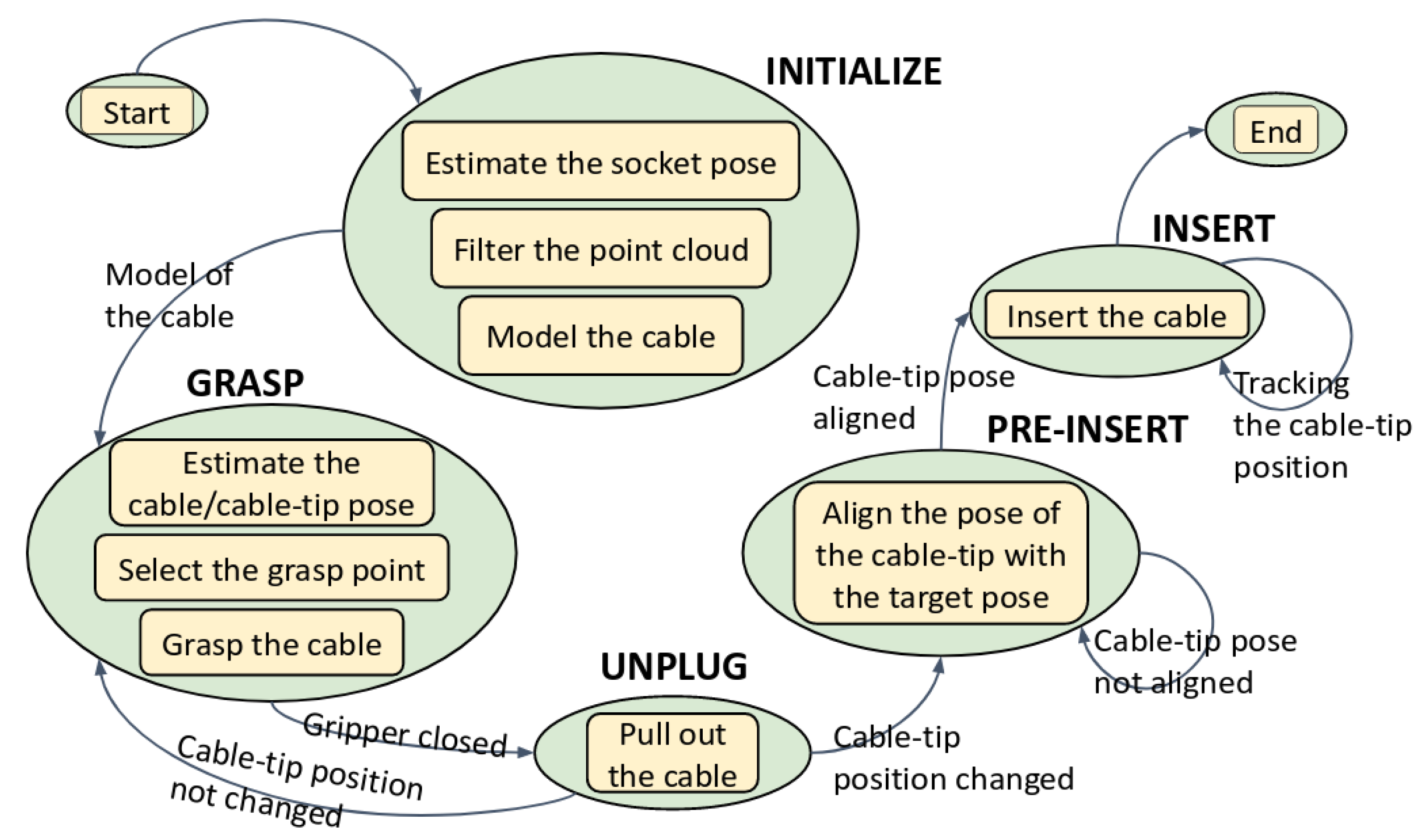
From a system design perspective, to complete the DRC Plug Task autonomously, the system needs to be able to model a linear flexible object, to keep track of the cable configurations and to detect the pose of the target socket through pose estimation, to plan motions for the robot, and to align the cable tip with the target socket by a controller. A flow of the proposed system architecture is presented in Figure 2.
We can divide the entire process into five phases: Initialize, Grasp, Unplug, Pre-insert, and Insert. Our goal is to give the robot the ability to automatically switch the phases. From the Initialize phase to the Grasp phase, the system needs to sense the environment, including estimating the socket pose, filtering the point cloud, and modeling the cable. After getting the model of the cable, the system will estimate the poses of the cable and the cable tip and select the grasp point on the cable. Then the robot will go and grasp the cable. From the Unplug phase to the Pre-insert phase, the robot needs to align the pose of the cable tip with the target pose. From the Grasp phase to the Unplug phase, a planned motion away from the target socket and perpendicular to the target socket hole plane is executed by the robot, and another planned motion perpendicular to the socket hole plane but close to the socket is executed by the robot to transfer from the Pre-insert phase to the Insert phase. To automate the DRC Plug Task, the robot needs to know where the target is. We used the Hough Circle Transform [30] to detect the hole (circle) of the target socket. Then the coordinates of the circle center can be obtained. By integrating the depth information at the circle center, we can get the 3D position of the target socket center. Random sample consensus (RANSAC) method [31] is applied to detect the wall plane which is parallel to the socket hole plane. The normal to the wall plane and the 3D position of the target center are used to define the target frame (named “Target_Socket”).

2.2. Geometrical Modeling of the Linear Flexible Objects

It is challenging to find specific irregular objects in a noisy environment. In this task, a real-time object detection method called YOLO [32] is used for detecting the flexible power cable in the 2D images (Figure 3(left)). The process requires training a convolutional neural network (CNN) with self-labeled images. We trained the network for 40,000 steps with 100 labeled images. The output of YOLO is a bounding box that narrows the region down to a search for the cable. To get the pixels corresponding to the object, we then use the color information and detect the black pixels in this region (Figure 3(middle)). These pixels are stored in a set in the order from top to bottom and left to right, and we define the middle pixel as the center pixel of the object which is marked as “Center” in Figure 3(left). By integrating the depth information, we can get the 3D positions of the object center. A PassThrough filter from the point cloud library (pcl) [33] was used to filter the point cloud from three dimensions as shown in Figure 3(right). The point cloud in the narrowed bounding box served to model the cable. It is published through ROS at a frequency of 30 Hz.
In Figure 3 (right), the remaining points in the filtered point cloud are shown in white with respect to the world frame. The x, y, and z axes of the world frame are represented by the red, green, and blue bars, respectively. Modeling the cable in 3D space is still a research problem in linear flexible object manipulation. On the other hand, modeling a curved line in 2D space is a solved problem. We can exploit this by projecting the 3D curve onto 2D spaces. In this study, we project the 3D point cloud onto the y-x and y-z planes. However, the projection in 2D may have multiple corresponding x or z values to the y coordinate. For example, if the cable has a “⊃” shape, in order to get a unique projection model, we filtered out the point cloud below the rightmost point. Moreover, we assume that the cable is not in more complex shapes, e.g., “S” or “ α ” shape. Due to the relatively high stiffness and large bending radius of the power cables, we found that a quadratic polynomial equation is sufficient to represent their shapes:
x = a 0 + a 1 y + a 2 y 2 ,
z = b 0 + b 1 y + b 2 y 2 .
The polynomial coefficients a 0 , a 1 , a 2 , b 0 , b 1 , and b 2 are estimated by using the least squares method, and they continuously change based on the shape of the power cable. In order to model the cable in 3D, we uniformly sample the points in Figure 3(right) along the y-axis. The corresponding x and z values can be calculated by using Equations (1) and (2). This projection method is efficient, and the model can be published through ROS at a frequency of 29.997 Hz.
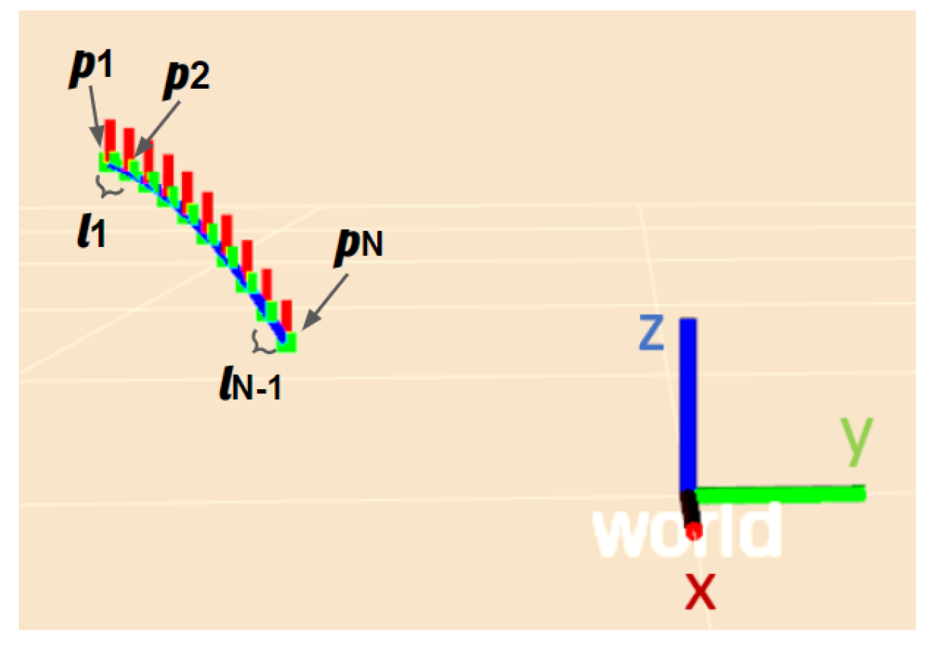
Figure 4 shows an example of modeling result with 10 sample points. The power cable is visualized in Rviz by markers. Green markers represent the sampling points, consecutive points are connected by blue lines, and vertical upward red lines are used to illustrate the displacements between the points.
In order for the robot to detect and track the location of the cable and cable tip, we propose a piece-wise linear model for the object. In Figure 4, we denote the leftmost point as p 1 and the remaining points as p 2 , p 3 , , p N from left to right, where N is the number of sample points. We denote the leftmost blue line that connects p 1 and p 2 as l 1 and rest of the blue lines as l 2 , l 3 , , l N 1 . We assume that the line l i is the tangent at the point p i . Because the cable tip has the round shape, its roll angle can be neglected (we set it to 0). After setting the point p 1 as the origin and defining the x axis to the tangent of the point p 1 , the “cable_tip” frame is defined in Figure 5(left).
Now that the positions of all the sample points and the pose of the cable tip are known with respect to the robot frame, a feasible grasp pose for the robot can be calculated to grasp the cable. Because the plug is inside the socket, we consider only the sampling points on the cable except the cable tip as the grasp point candidates. To select the grasp point on the cable, the following trade-off needs to be taken into account. As the grasp point gets closer to the cable tip, the risk of the robot colliding with the socket or the wall increases and the number of points in the filtered point cloud reduces. On the other hand, when the grasp point is too far away from the cable tip, the robot can not align the cable tip pose with the target socket pose because the cable will dangle substantially. Thus, the grasp point needs to be selected empirically to meet these two constraints. For this purpose, we pre-define a minimum distance from the grasp point to the cable tip ( p 1 ) along the cable as d m i n , and a maximum distance as d m a x . d m i n and d m a x are pre-defined with the robot holding the cable before the experiment. With this step, the cable deformation characteristics can be ignored for selecting the grasp point, and this vision-only method is satisfied for selecting a feasible grasp point. Since we can calculate the length of the lines l 1 , , l N 1 , we can also calculate the distance d s from each sampling point to the cable tip by using:
d s i = 1 s l i , s = 1 , , N 1 .
The grasp point needs to be selected such that d s [ d m i n , d m a x ] for the robot to be able to align the cable tip pose with the target pose. By using the same method of estimating the “cable_tip” frame, we can get the “cable” frame (Figure 5(right)), which is used to get the grasp pose of the robot’s end-effector. The grasp pose is then used as the target of the motion planner. We implemented both MoveIt! [34] and TrajOpt [35] for the motion planing in this task.
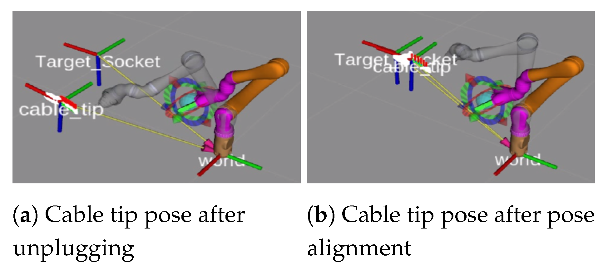
Once grasping of the cable is completed, a pulling motion along the y axis of the “world” frame is generated to unplug the cable. Figure 6a shows the “cable_tip” frame after the robot unplugs the power cable. We filter out the point cloud of the plug during modeling which improves the accuracy of the model because the plug is a straight and rigid object.

2.3. Pose Alignment Controller

In order to finish the insertion task, the robot needs to adjust the pose of the cable tip to match with the pose of the target socket. A pre-insert frame right in front of the target socket is defined as our target pose for the pose alignment controller. Because of the continuous visual feedback, we decide to use the visual servoing approach to align the cable tip pose with the target socket pose.
To explain this algorithm in a succinct way, we denote the transformation matrix from the “cable_tip” frame to the pre-insert frame as T c t p r e , the transformation matrix from the pre-insert frame to the “end-effector” frame as T p r e e e , the transformation matrix from the “cable_tip” frame to the “end-effector” frame as T c t e e .
[ Δ x Δ y Δ z Δ α Δ β Δ γ ] are the translational (x, y, z) and rotational ( r o l l , p i t c h , y a w ) deviations between the “cable_tip” frame and the pre-insert frame under the “end-effector” frame which can be calculated as
Δ x Δ y Δ z = x 1 y 1 z 1 x 2 y 2 z 2 , Δ α Δ β Δ γ = α 1 β 1 γ 1 α 2 β 2 γ 2 ,
where x 1 , y 1 , z 1 , α 1 , β 1 , and γ 1 are translational and rotational terms from the transformation T p r e e e under the “end-effector” frame, x 2 , y 2 , z 2 , α 2 , β 2 , and γ 2 are translational and rotational terms from the transformation T c t e e under the “end-effector” frame.
Then the linear and angular velocities under the “end-effector” frame can be calculated [36]:
x ˙ y ˙ z ˙ = Δ x Δ y Δ z 1 Δ t ,
w x w y w z = 1 0 s i n ( Δ β ) 0 c o s ( Δ α ) c o s ( Δ β ) s i n ( Δ α ) 0 s i n ( Δ α ) c o s ( Δ β ) c o s ( Δ α ) Δ α Δ β Δ γ 1 Δ t ,
where Δ t is the execution time, x ˙ , y ˙ , z ˙ , w x , w y , a n d w z are linear and angular velocities under the “end-effector” frame, which will be used as inputs for our PD controller.
A PD controller was designed to calculate the Cartesian velocity ( x ˙ ) for the robot’s end-effector:
x ˙ = K p e + K d e ˙ ,
where e is the error, which is [ x ˙ y ˙ z ˙ w x w y w z ] , K p and K d are proportional and derivative terms. Our designed values for K p and K d are 2.0 and 0.2.
After getting the Cartesian velocity from our PD controller, a velocity controller built in the Jaco robotic arm generates the controlled joint velocity ( q ˙ ) by using robot Jacobian matrix ( J ):
q ˙ = J 1 x ˙ .
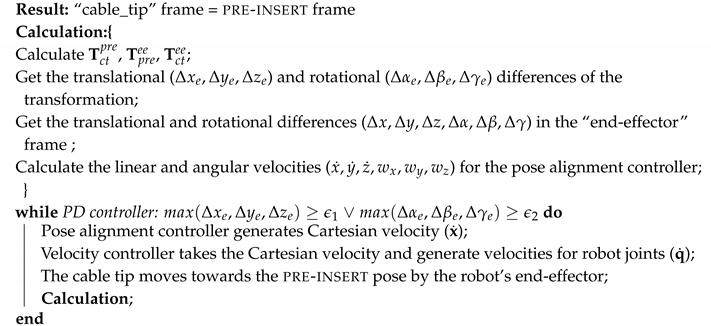
Algorithm 1 shows the pose alignment control loop. The control loop keeps running until the translational deviations ( Δ x e , Δ y e , Δ z e ) and the rotational deviations ( Δ α e , Δ β e , Δ γ e ) from the “cable_tip” frame to the pre-insert frame ( T c t p r e ) satisfy the thresholds which are ϵ 1 (m) and ϵ 2 ( r a d ). A successful example of the robot aligning the cable to pre-insert frame is shown in Figure 6b. For the final insertion step, a translation along the x axis of the “cable_tip” frame is applied. The insertion is facilitated by the magnets on the plug and in the socket.
Algorithm 1: Pose alignment algorithm
Machines 08 00046 i001

3. Task Automation in Simulation Based on Our Physical Model of the Linear Flexible Objects

Simulation plays a very important role in robotics [37]. Various simulators (e.g., Gazebo, OpenRAVE, MuJoCo) are used to design the robot model, create different simulation environments, analyze the kinematics and dynamics of the robot, design different plan or control algorithms, investigate the performances of the system, etc. The construction of a real environment is usually more expensive than building a simulation environment. In simulation, we can build objects with their geometric and physical properties. We can also design new robot models or import existing robot models to complete a series of manipulation tasks. Usually, the robot needs to make physical contact with the environment and objects when completing the manipulation tasks. Learning to use the robot to manipulate objects in simulation can help with avoiding damage to the robot, the environment, and humans.
The DARPA Robotics Challenge (DRC) is a competition funded by the US Defense Advanced Research Projects Agency between 2012 and 2015. The DARPA Robotics Challenge (DRC) Simulator (DRCSim) and the Space Robotics Challenge Simulation (SRCSim) have related open-source simulations for most tasks in the competition. However, the Plug Task used in the 2015 DARPA Robotics Challenge Finals does not have a complete simulation environment. Based on our group’s prior experience in this competition [14] and the detailed definition and requirements of this task, we decided to build a complete simulation environment and complete this task in simulation for our research study.

3.1. Simulation Environment Setup

The simulation setup consists of a wall, two power sockets, a power cable with a plug, a Kinova Jaco V2 robotic arm, and a Kinect camera. Figure 7 shows the simulation setup in the Gazebo simulator [38]. Modeling of rigid objects in the simulator is a solved problem: The wall can be modeled as a box and the plug can be fitted as a cylinder. Modeling objects of irregular shape is relatively difficult, but we can get the model in a solid modeling computer-aided design tool (e.g., SolidWorks) and then use a converter (e.g., SolidWorks to URDF Exporter) to get the model in the desired format. The RGB-D camera in the simulated environment is a Kinect camera. To read the point cloud information, we need to model the Kinect camera as a Depth Camera Plugin in Gazebo. The simulated Jaco arm is cloned from the official Kinova GitHub website. In simulation, we assume that the positions of the sockets are known. Modeling of the cable in the simulator is a challenge and it will be introduced in the next subsection.

3.2. Physical Model of the Linear Flexible Objects

Inspired by the “fire hose” model in Gazebo and the Piecewise Constant Curvature (PCC) model [39], a Dynamically-Consistent Augmented Formulation [40] of the PCC cable model is created in Figure 8a. A Gazebo model of the cable is also built based on the PCC model (see Figure 8b). Fifteen links are used to model the cable, each link is 5 cm long and weighs 50 g with the center of mass in the middle of the arc. The plug is also a link with length 10 cm and weight 100 g. These links are connected by revolute joints (except the joint between the plug and link-1) with the roll and pitch rotations. Each joint has stiffness and damping properties. There exists a trade-off in selecting the number of links for the simulated cable. In theory, more links of the cable model will produce more accurate simulation results. On the other hand, more links will cause the computing speed to slow down or even the simulator to crash. We observed that if the number of links is increased to twenty, sometimes there exists a misalignment between the links.

3.3. Sim2Real2Sim—Achieving Flexible Object Manipulation in Simulation with Identified Physical Model

The gap between simulation and real world was introduced in Simulation-to-Real (Sim2Real) [41,42,43,44]. Simulation is observed to have inevitable simplifications with heavy optimization. Besides, there exist physical events not modeled in simulators and parameters of the simulated models that need to be identified. Therefore, policies or parameters learned [45] and controllers designed [43] in simulation can not be transferred to the real world directly.
To reduce the gap between simulation and real world especially in flexible object manipulation, we propose a new strategy called Simulation-to-Real-to-Simulation (Sim2Real2Sim). Figure 9 shows the flowchart of the Sim2Real2Sim strategy we will use for bridging the gap. We start with a rough simulation environment with the estimated models. Then we test the system framework in the real world based on the methods developed in simulation and collect the data from the real world. Finally, we go back to the simulation and update the models and methods based on the data from the real world.
The research approach from simulation to real world implementation is widely applied in humanoid robot [46], mobile robot [47], robotic arm [48], etc. Normally, we complete a task in simulation first, then transfer the methods used in simulation to the real world. This step is named “simulation to real world” in the Sim2Real2Sim strategy. Building a simulation environment with all rigid objects is well-developed and these objects have nearly the same behavior in simulation and real world. However, simulation of soft objects usually simplifies the model; the gap between simulation and real world can not be ignored. Our proposed Sim2Real2Sim approach is for solving this issue. More specifically, we use real world data to improve the simulated models and we call this step “real world to simulation”. Therefore, our idea of Sim2Real2Sim is like a research strategy and a generalized methodology to reduce the gap between simulation and the real world and to obtain a high-fidelity simulation environment for flexible object manipulation.

3.3.1. Simulation to Real World

Led by the Sim2Real2Sim strategy, we build an initial simulation environment based on the task requirements (see Figure 7). Recall that the DRC Plug Task can be divided into five phases (Initialize, Grasp, Unplug, Pre-insert, and Insert). In the Initialize and Grasp phases, we use the same geometrical model of the cable mentioned in Section 2.2 to estimate the cable tip pose and select the grasp point. After completing the Grasp of the cable in simulation with 30 successful experiments, we apply the same motion planning method to the real robot, and as expected, the real robot can Grasp the cable at the grasp point autonomously.
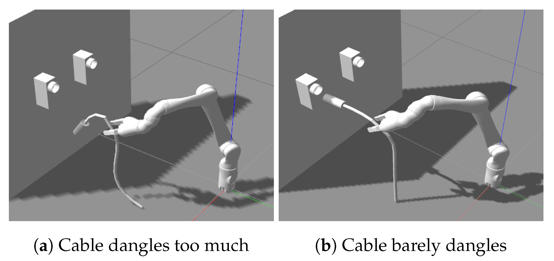
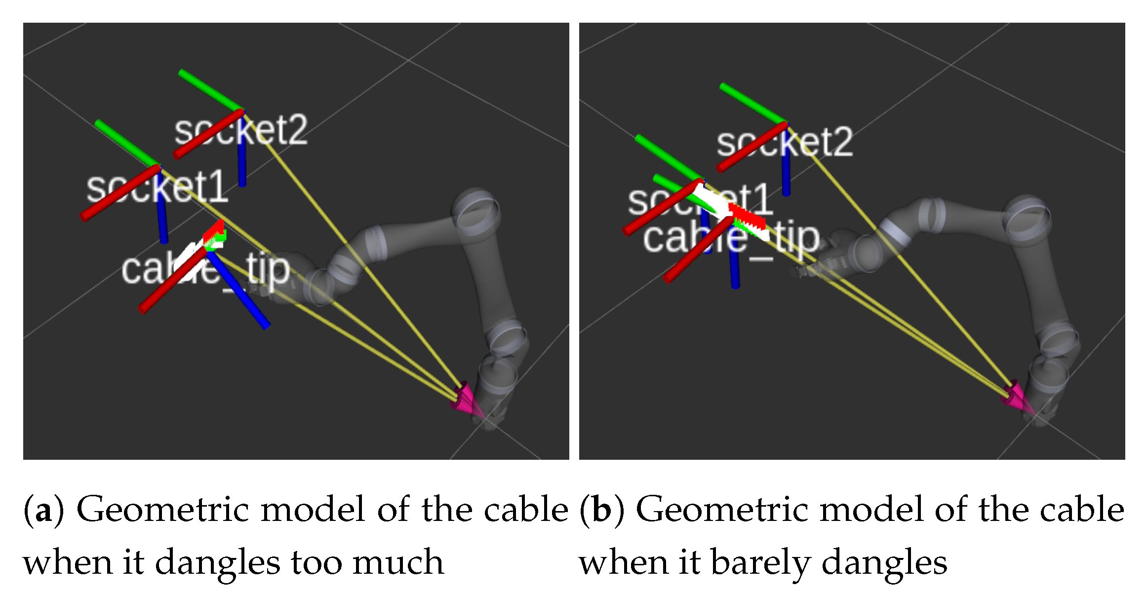
Unplugging the cable from the socket is straightforward with a backward panning motion for the end-effector. After the cable being plugged out of the socket, the weight of the front section (plug) of the cable will cause the cable to dangle. In our model (see Figure 8), this deformation depends on the joint stiffness and damping. We observe that the deformation of the cable is different by randomly setting the values for the joint stiffness and damping. Two special cases are: (1) The cable dangles too much (see Figure 10a); (2) the cable barely dangles (see Figure 10b). However, our geometric model works well in both cases (see Figure 11). To get reasonable values for the joint stiffness and damping and to narrow the gap between simulation and real world, we need to collect data from the real world and go back to simulation to update the models and methods. To automate the Plug Task, we need to figure out how to carry the cable to the Pre-insert position after the cable being Unplugged from the original socket. We use the visual servoing approach mentioned in Section 2.3 to reduce the differences between the “cable_tip” frame and the Pre-insert frame. After the cable tip moves to the Pre-insert position, a forward panning motion for the end-effector will Insert the cable tip (plug) to the target socket.

3.3.2. Real World to Simulation

After implementing the methods developed in simulation to real world, we realized that the deformation of the cable in simulation and real world is different after the robot unplugs the cable from the socket, which means our physical model in simulation needs to be tuned to match with the real world.
As we mentioned before, the cable is modeled as a rigid manipulator with passive revolute joints (see Figure 8). The dynamics of the cable can be represented as:
M q ¨ + C q ˙ + G + J T f e x t + K q + D q ˙ = τ ,
where q , q ˙ , q ¨ represent joint position, velocity, and acceleration. M is the inertia matrix. C is the centrifugal and Coriolis forces matrix. G is gravitational forces or torques. J T is the transpose of the robot Jacobian. f e x t is the external force. K is the stiffness and D is the damping. τ is a vector of joint torques, corresponding to the torques and forces applied by the actuators at the joints. Our goal is to estimate the stiffness and damping in this equation.
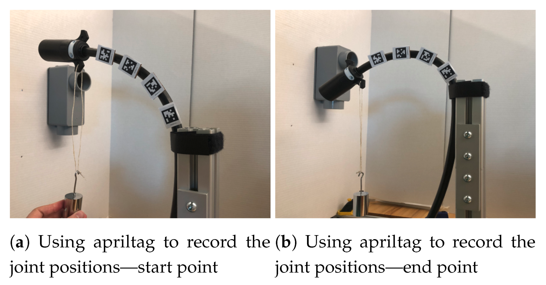
Recalling that each joint of the cable has roll and pitch rotations (see Figure 8), we simplify the model by only considering the pitch. Our first challenge is to get the joint values. AprilTag [49] is used for getting the joint positions. Figure 12 shows the start and end points of recording the joint positions with a 100 g weight added to the tip. Four apriltags with side lengths of 2.0 cm [50] are attached on the cable 5 cm apart (same as the link length in Gazebo). The joint position q and the time stamp are recorded for calculating joint velocity q ˙ and acceleration q ¨ . After we get joint values, the robot Jacobian J can be calculated. Because the joints on the cable are passive, τ equals to 0 . The external force f e x t is also known by multiplying the mass of the weight (0.1 kg) with the gravitational acceleration (9.8 m/s 2 ).
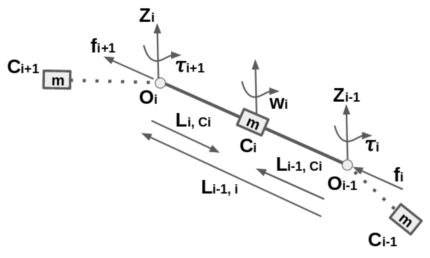
Computing of the left three terms ( M q ¨ + C q ˙ + G ) in Equation (9) is our second challenge. We refer to the Recursive Newton Euler (RNE) approach [51,52,53]. The RNE approach includes two recursions: Forward recursion for computing velocities and accelerations, and backward recursion for computing forces and torques. Figure 13 shows the parameters of three adjacent links and Algorithm 2 shows the detailed RNE algorithm. The RNE algorithm gives us the torque required for each joint to overcome the gravity of the model and the force generated from the motion if the cable joints have no friction or damping and there is no external force. The left three terms ( M q ¨ + C q ˙ + G ) in Equation (9) can be represented as:
M q ¨ + C q ˙ + G = τ R N E ,
where τ R N E equals to [ τ 1 , τ 2 , τ n ] T ( n = 4 ) calculated from the RNE method.
Algorithm 2: Recursive Newton Euler algorithm
Forward recursion:{
Initial: Velocity and acceleration of the base link both equal to 0
Compute link angular velocity: w i = ( R i i 1 ) T ( w i 1 + q ˙ i z i 1 )
Compute link angular acceleration: w ˙ i = ( R i i 1 ) T ( w ˙ i 1 + q ¨ i z i 1 + q ˙ i w i 1 × z i 1 )
Compute linear acceleration of origin of frame i:
a i = ( R i i 1 ) T a i 1 + w ˙ i × L i 1 , i + w i × ( w i × L i 1 , i )
Compute linear acceleration of centre of C i : a c i = a i + w ˙ i × L i , c i + w i × ( w i × L i , c i ) }
Backward recursion:{
Compute force exerted by link i 1 on link i: f i = R i + 1 i f i + 1 + m i a c i
Compute moment exerted by link i 1 on link i:
μ i = f i × ( L i 1 , i + L i , c i ) + μ i + 1 + f i + 1 × L i , c i + I i w ˙ i + w i × ( I i w i )
Compute torque exerted by link i 1 on link i: τ i = μ i T z i 1 + τ i n e r t i a }
OpenRAVE [54] is used for computing the robot Jacobian J and the inverse dynamic terms M q ¨ + C q ˙ + G . Figure 14 shows the physical model built in OpenRAVE. We pick the first four links of the cable for modeling because the cable tip pose is not guaranteed to be aligned with the socket pose if the grasp point is beyond this range. The robot Jacobian and inverse dynamics are computed based on this model.
At this point, we can rewrite Equation (9) as:
K q + D q ˙ = τ ( M q ¨ + C q ˙ + G + J T f e x t ) .
The terms to the right of the Equation (11) are known. To get the stiffness K, we use the robot configuration when the joint velocity q ˙ equals to 0 . In our case, we use the joint values when the cable is finally stationary after adding the weight (see Figure 12b). The stiffness K can be computed by using Equation (12) with q ˙ = 0 ,
K = ( τ ( M q ¨ + C q ˙ + G + J T f e x t + D q ˙ ) ) q + ,
where q + is the pseudoinverse of q .
After getting stiffness K, we take it to Equation (11). The damping D can then be calculated as:
D = ( τ ( M q ¨ + C q ˙ + G + J T f e x t + K q ) ) q ˙ + ,
where q ˙ + is the pseudo inverse of q ˙ . Unlike the calculation for stiffness, we use joint values prior to the cable entering its final stationary position to ensure that joint velocity is not 0 .
Finally, we update the Gazebo model based on the calculated stiffness and damping. Recalling that each joint on the cable also has the roll rotation. We can use the same method to identify the stiffness and damping properties if we can figure out how to add a constant twist torque on the cable tip. This part is left as future work. Currently, we use the joint limits to set the roll rotation based on the observation. Figure 15 shows the deformation of the cable with the updated model parameters in the simulation. Detailed comparison of the model deformation in simulation with the cable deformation in the real world will be discussed in Section 4.

4. Experiments and Results

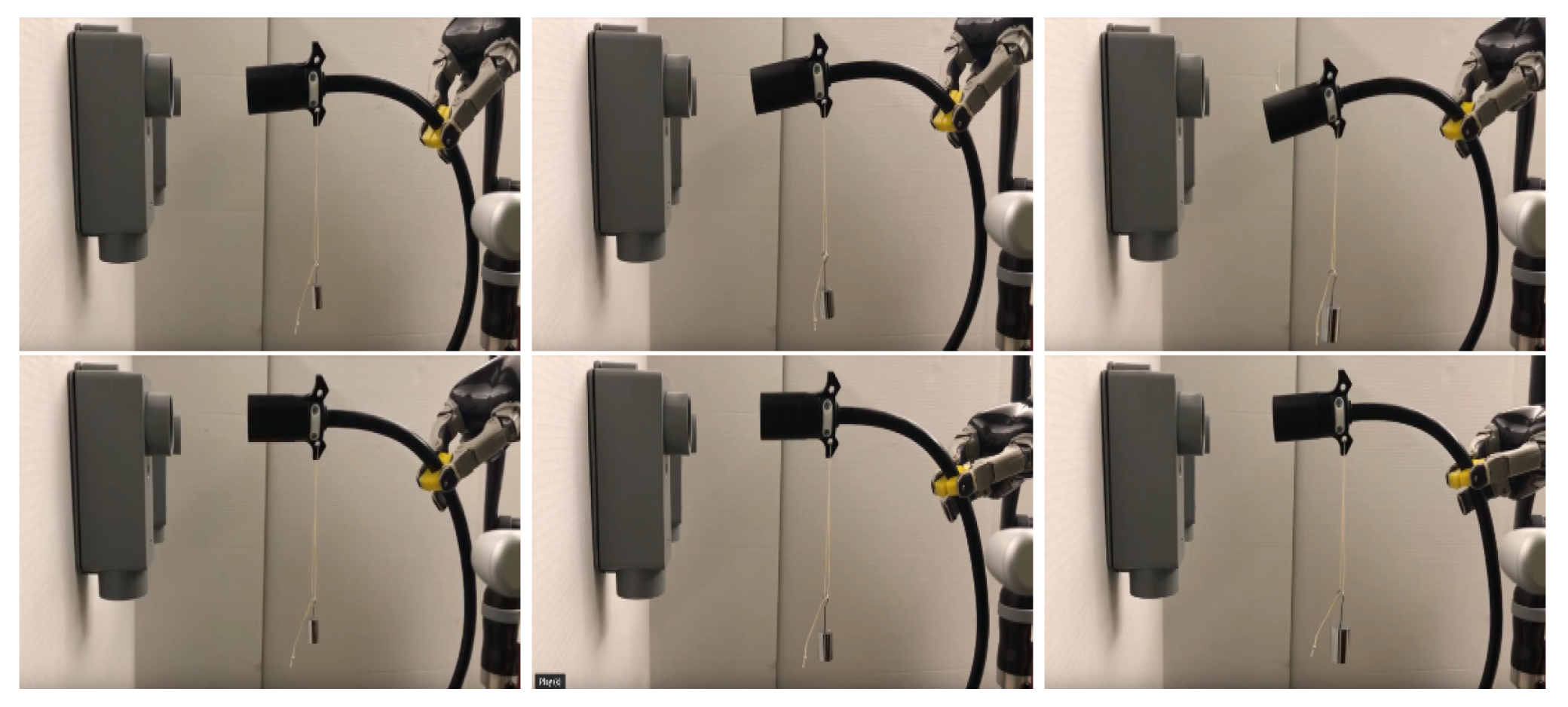
Our system framework for task automation is evaluated by running the DRC Plug Task both in simulation and real world for 20 trials. In simulation, the average completion time is 66.25 s with an average real-time factor: 0.65. Figure 16 shows the robot completing the DRC Plug Task in simulation. In real world, the average completion time is 31.53 s. Figure 17 shows the robot completing the DRC Plug Task in the real world. We also test our automation approach with a different robot platform which is a Kinova Gen3 7-DOF arm. Figure 18 shows the Gen3 robot arm completing the DRC Plug Task in the real world. In order to validate the performance of our geometrical modeling of the cable, pose alignment controller, and the cable model in simulation, we conduct different experiments in each aspect.

4.1. Validation of the Geometrical Modeling of the Cable and the Pose Alignment Controller

To validate the performance of our modeling method and pose alignment controller, we implement three experiments. The first experiment is for testing the grasp functionality with different initial poses of the cable. The second experiment shows the performance of the pose alignment controller with two different cables. The last experiment shows the robustness of our pose alignment controller under external disturbances.
The first experiment is for testing the grasp functionality with different initial poses of the cable modeled by our geometrical modeling method. Recalling the trade-off mentioned in Section 2.2, we need to pick values of d m i n and d m a x for different cables. For the power cable (with plug), we define d m i n = 18 cm and d m a x = 30 cm. For the HDMI cable, these parameters are selected as d m i n = 12 cm and d m a x = 24 cm. Our method will prioritize the sample point closest to the midpoint in this range as grasp point when performing tasks. Figure 19 shows the robot is able to grasp the cable with three different initial states. Figure 20 shows the modeling of the cable for these three different initial poses. Table 1 shows the model parameters for these states.
The second experiment shows the performance of the pose alignment controller with two different cables. Due to the limitation of point cloud publishing frequency (30 Hz), we set the constraints for linear and angular velocities in the Cartesian space as 1.5 m/s and 0.6 rad/s to prevent the substantial deformation of the cable in the interval of the point cloud update. We implement the pose alignment controller with two different cables (10 trials/each). Figure 21 shows two successful runs during these experiments. Figure 22 shows the pose differences between the cable tip frame and the pre-insert frame. Our pose adjustment control loop ends when the pose differences meet the thresholds which is 0.01 m for translational terms and 0.02 rad for rotational terms. In this experiment, we conclude that the HDMI cable (average elapsed time: 12.26 s) needs more time than the power cable (average elapsed time: 5.59 s) to adjust the pose. A potential reason might be that the HDMI cable has more deformation than the power cable.
Another experiment is performed for evaluating the robustness of the pose alignment controller by adding disturbances to the pose alignment control loop and testing whether our algorithm can still achieve the target. Figure 23 shows that different disturbances added to the cable tip while the system is in the pose alignment loop and the final pose of the cable after the loop, which demonstrates that our pose alignment controller is able to resist such external disturbances.
These results demonstrate that our method for modeling linear flexible objects can provide a 3D model with adaptive parameters based on the visual feedback. This model is capable of representing various shapes of the cable during the Plug Task. More importantly, our pose alignment algorithm is robust to handle different cable-like objects and is capable of resisting disturbances.

4.2. Validation of the Cable Model in Simulation

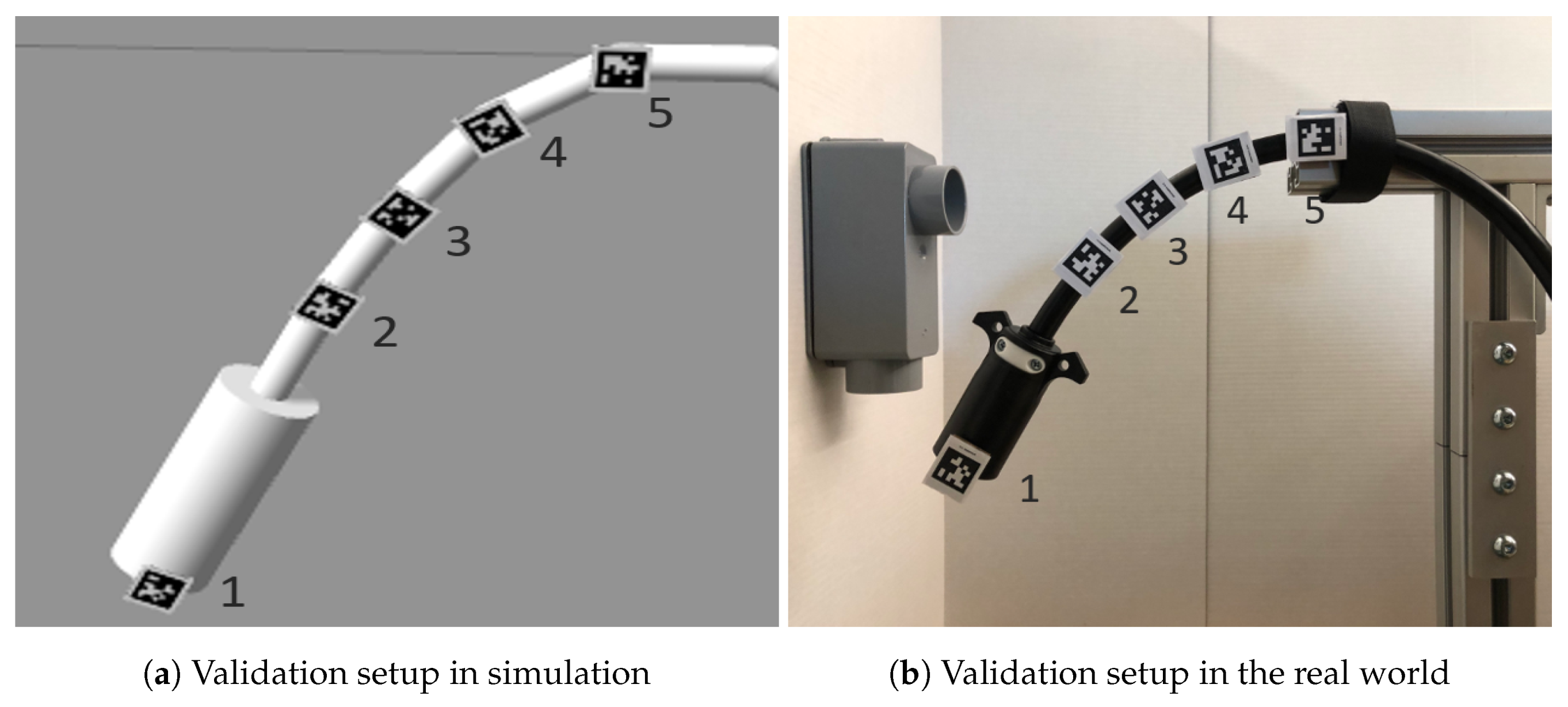
To validate the model in simulation, we designed two experiments. First, we fix the same link on the cable to the world, and compare the joint positions of the cable in simulation and real world. Second, we fix different links on the cable horizontally, and compare the pose of the cable tip in simulation and real world. In simulation, the link of the simulated cable can be fixed to the world by adding a “fixed” joint connecting the “world” link and the link you want to fix. In real world, we fix the cable by using a zip-tie. Figure 24 shows the setup in simulation and real world for comparison of the cable deformation. Apriltags are attached to the cable tip and on the first four revolute joints to get the transformation at each joint. Figure 25 shows the visualized frames in Rviz, and the “tag_1” frame is equivalent to the “cable_tip” frame.
Our first experiment is comparing the deformation of the cable by fixing the same link horizontally to the world. We use the setup in Figure 24 and obtain the frames (“tag_1”, “tag_2”, …, “tag_5”) both in simulation and real world (see Figure 25). Transformations of these frames are used to get the joint positions for the comparison in simulation and real world. We first compare the joint positions of the cable with no external force, then we add different weights to the cable tip and compare the differences of the joint positions under these disturbances.
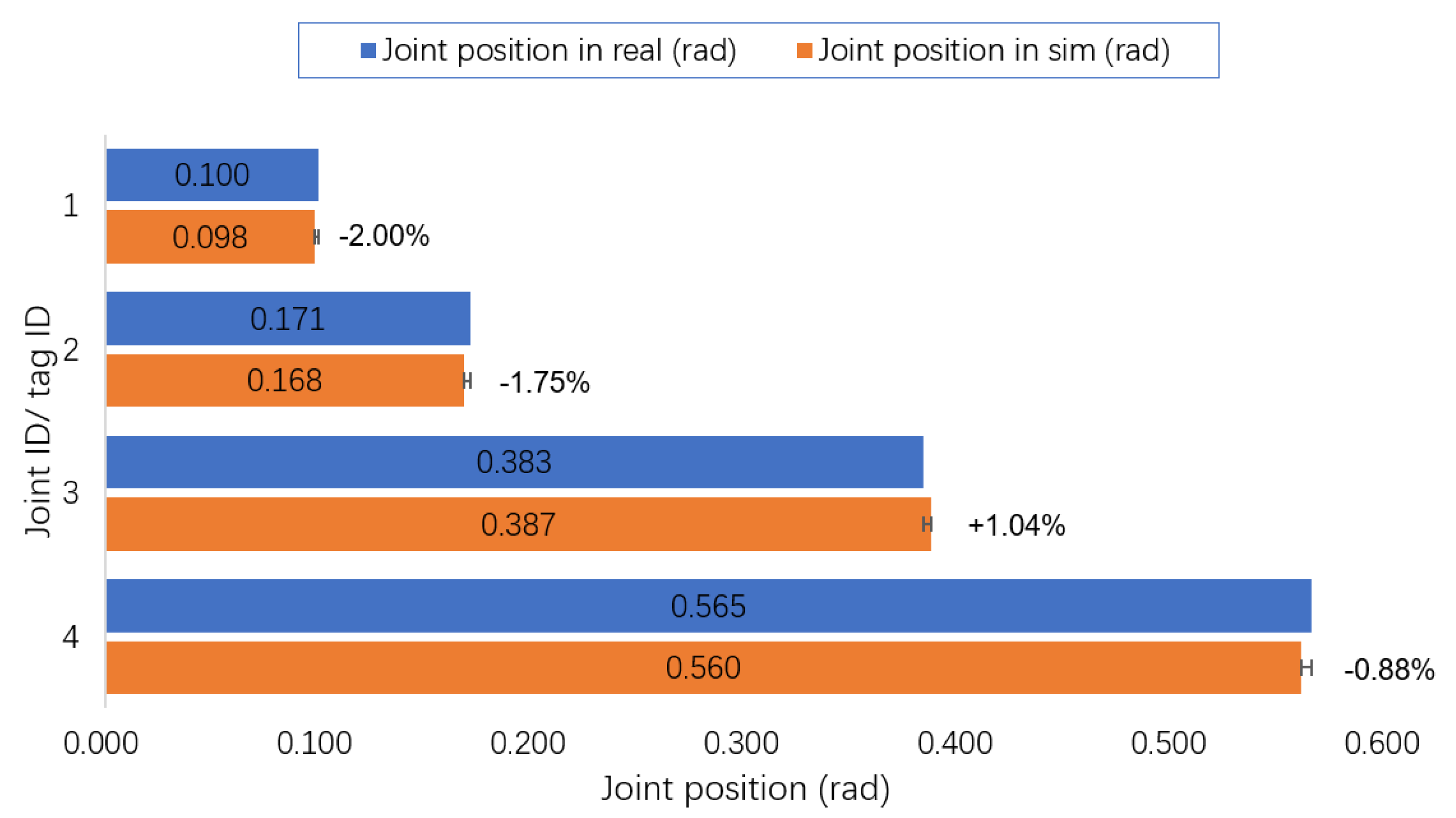
Figure 26 shows the comparison result by fixing the link-5 (the link after tag-5) on the cable to the world. From the Figure 26, we conclude that the shape of the cable in the simulation is close to the real cable with the largest difference of the joint positions being 0.005 rad, and the largest percent error between the simulation and the real world is 2.00%. To test the simulation model with external disturbances, we add two different weights (50 g and 100 g) to the cable tip, and we compare the joint positions of the simulated cable with the one of the real cable (see Figure 27 and Figure 28). The percent errors are reasonable which proves the accuracy of our simulated cable model.
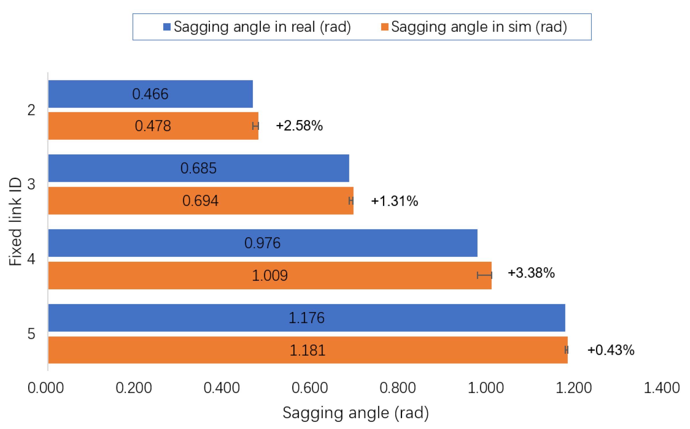
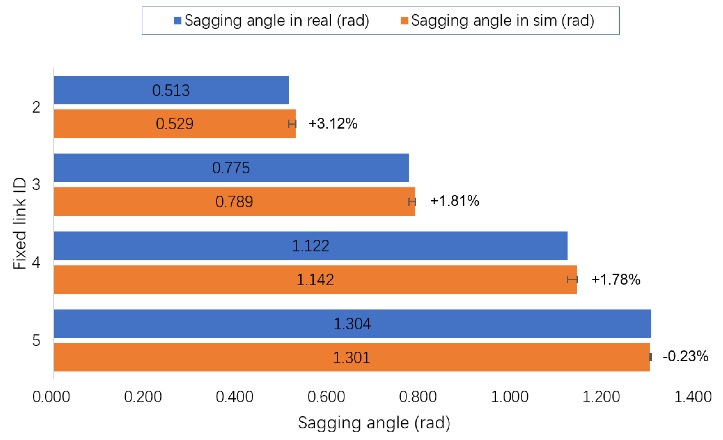
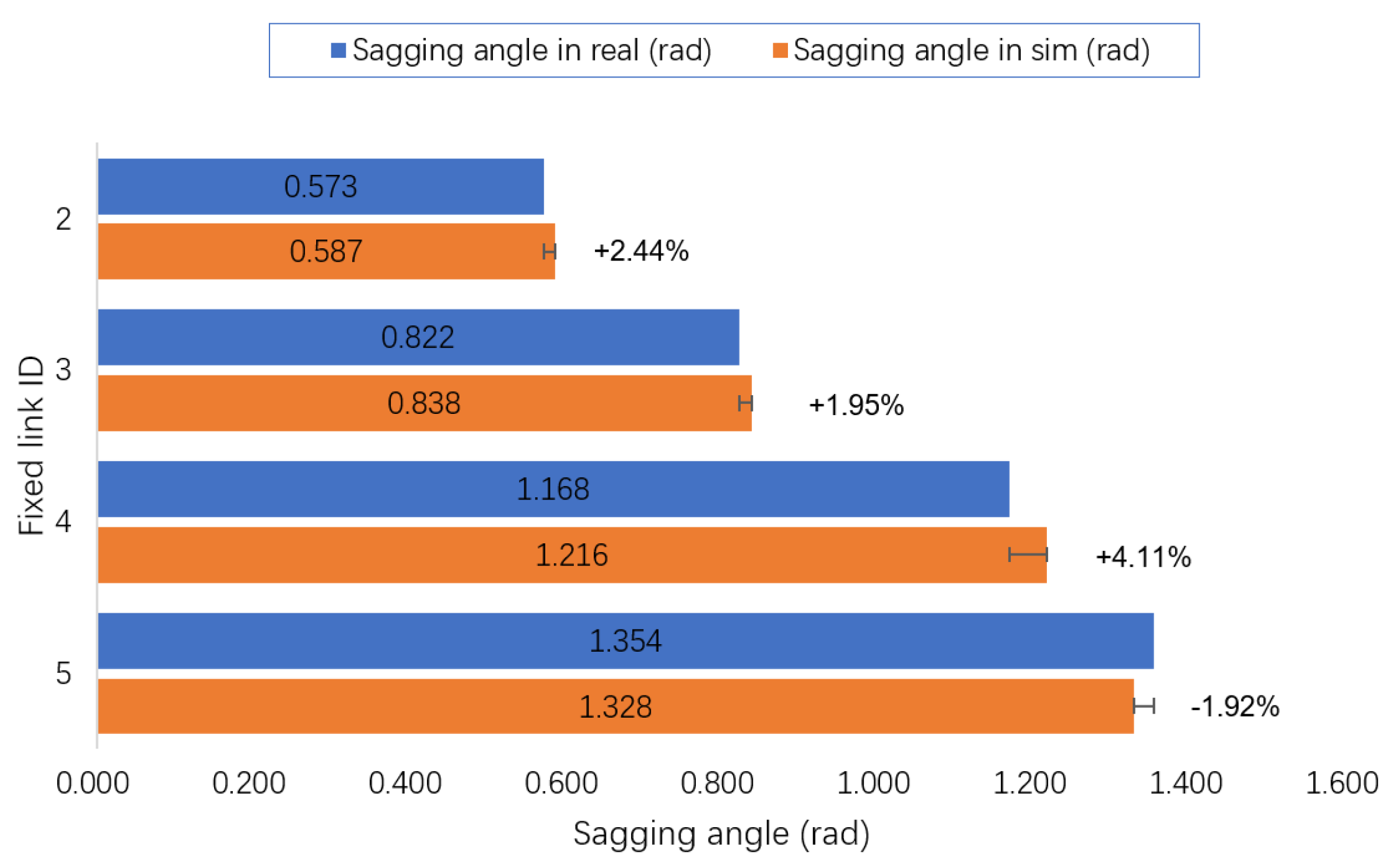
Our second experiment is fixing different links on the cable horizontally to the world in simulation and real world to compare the deformation of the cable tip. We compare the rotation angles around the z-axis from the frame we have fixed to the world to frame “tag_1”. This experiment is to compare the sagging angle of the cable tip in simulation and real world. Similar to the first experiment, three comparisons are made for validation.
Figure 29 shows the comparison result by fixing different links on the cable to the world. From the Figure 29, we conclude that the difference of the sagging angle between the simulation model and real cable is within a reasonable range (<0.04 rad), and the largest percent error is 3.38%.
We also run this experiment with two different weights (50 g and 100 g) added to the cable tip. Figure 30 and Figure 31 show the results. In the case of a 50 g weight added to the cable tip, the maximum difference of the cable sagging angle between the simulation and the real world is 0.02 rad, and the largest percent error is 3.12%. If a 100 g weight is added to the cable tip, the maximum difference of the cable sagging angle between the simulation and the real world is 0.048 rad, and the largest percent error is 4.11%.

5. Conclusions

In this paper, we proposed a geometrical modeling method based on the curves on two projection planes for linear flexible objects subject to gravity. The geometrical model enables tracking the 3D curvature of the linear flexible object, the pose of the tip and the pose of the selected grasp point on the object. A robust pose alignment controller based on the geometrical model with adaptive parameters can bring the cable tip to a desired pre-insert position. We designed and used an autonomous system pipeline with our formulated methods to accomplish the DRC Plug Task autonomously.
We also proposed a new strategy called Sim2Real2Sim. This strategy includes two procedures: sim-to-real and real-to-sim. The sim-to-real procedure is to organize the methods used in simulation and apply them to the real world in a reasonable way. The real-to-sim procedure is for updating the models in simulation which bridges the gap between simulation and real world. A novel identification method based on inverse dynamics is implemented to update the parameters of the simulated flexible objects. The comparison of the deformation of the flexible objects in simulation and real world proves the accuracy of the model in the simulation
The success of the system framework running both in simulation and the real world demonstrates the practicability and reliability of our proposed methods. Possible future work includes: (1) Explore different model representations of the cable shapes in the case of more complex deformations; (2) apply our approach to different robot platforms (e.g., a dual-arm system) or to other flexible object manipulation tasks (e.g., a cable routing assembly task); (3) get more evaluations on our Sim2Real2Sim strategy; (4) update the simulation model for the linear flexible objects by adding more degrees of freedom (e.g., using more apriltags); (5) bring the material and friction information from the real world to the simulation to obtain a more close-to-reality simulated cable model and a better simulation when the cable makes contact with the environment.

Author Contributions

Methodology, P.C. and T.P.; Software, P.C.; Supervision, T.P.; Validation, P.C. and T.P.; Writing—original draft, P.C.; Writing—review & editing, P.C. and T.P. All authors have read and agreed to the published version of the manuscript.

Funding

This research is supported by the National Aeronautics and Space Administration under Grant No. NNX16AC48A issued through the Science and Technology Mission Directorate, by the National Science Foundation under Award No. 1451427, 1544895, 1928654, 1935337, 1944453 and by the Office of the Secretary of Defense under Agreement Number W911NF-17-3-0004.

Conflicts of Interest

The authors declare no conflict of interest. The funders had no role in the design of the study; in the collection, analyses, or interpretation of data; in the writing of the manuscript, or in the decision to publish the results.

References

  1. Sanchez, J.; Corrales, J.A.; Bouzgarrou, B.C.; Mezouar, Y. Robotic manipulation and sensing of deformable objects in domestic and industrial applications: A survey. Int. J. Robot. Res. 2018, 37, 688–716. [Google Scholar] [CrossRef]
  2. Lee, A.X.; Lu, H.; Gupta, A.; Levine, S.; Abbeel, P. Learning force-based manipulation of deformable objects from multiple demonstrations. In Proceedings of the 2015 IEEE International Conference on Robotics and Automation (ICRA), Washington, DC, USA, 26–30 May 2015; pp. 177–184. [Google Scholar]
  3. Nair, A.; Chen, D.; Agrawal, P.; Isola, P.; Abbeel, P.; Malik, J.; Levine, S. Combining self-supervised learning and imitation for vision-based rope manipulation. In Proceedings of the 2017 IEEE International Conference on Robotics and Automation (ICRA), Singapore, 29 May–3 June 2017; pp. 2146–2153. [Google Scholar]
  4. Miller, S.; Van Den Berg, J.; Fritz, M.; Darrell, T.; Goldberg, K.; Abbeel, P. A geometric approach to robotic laundry folding. Int. J. Robot. Res. 2012, 31, 249–267. [Google Scholar] [CrossRef]
  5. Mallapragada, V.; Sarkar, N.; Podder, T.K. Toward a robot-assisted breast intervention system. IEEE/ASME Trans. Mechatron. 2011, 16, 1011–1020. [Google Scholar] [CrossRef]
  6. White, J.R.; Satterlee, P.E., Jr.; Walker, K.L.; Harvey, H.W. Remotely Controlled and/or Powered Mobile Robot with Cable Management Arrangement. U.S. Patent 4,736,826, 12 April 1988. [Google Scholar]
  7. Tang, T.; Wang, C.; Tomizuka, M. A framework for manipulating deformable linear objects by coherent point drift. IEEE Robot. Autom. Lett. 2018, 3, 3426–3433. [Google Scholar] [CrossRef]
  8. Wang, W.; Berenson, D.; Balkcom, D. An online method for tight-tolerance insertion tasks for string and rope. In Proceedings of the 2015 IEEE International Conference on Robotics and Automation (ICRA), Washington, DC, USA, 26–30 May 2015; pp. 2488–2495. [Google Scholar]
  9. Lui, W.H.; Saxena, A. Tangled: Learning to untangle ropes with rgb-d perception. In Proceedings of the 2013 IEEE/RSJ International Conference on Intelligent Robots and Systems, Tokyo, Japan, 3–7 November 2013; pp. 837–844. [Google Scholar]
  10. Papacharalampopoulos, A.; Makris, S.; Bitzios, A.; Chryssolouris, G. Prediction of cabling shape during robotic manipulation. Int. J. Adv. Manuf. Technol. 2016, 82, 123–132. [Google Scholar] [CrossRef] [Green Version]
  11. Zhu, J.; Navarro, B.; Fraisse, P.; Crosnier, A.; Cherubini, A. Dual-arm robotic manipulation of flexible cables. In Proceedings of the 2018 IEEE/RSJ International Conference on Intelligent Robots and Systems (IROS), Madrid, Spain, 1–5 October 2018; pp. 479–484. [Google Scholar]
  12. Spenko, M.; Buerger, S.; Iagnemma, K. The DARPA Robotics Challenge Finals: Humanoid Robots to the Rescue; Springer: Berlin, Germany, 2018; Volume 121. [Google Scholar]
  13. Cisneros, R.; Nakaoka, S.; Morisawa, M.; Kaneko, K.; Kajita, S.; Sakaguchi, T.; Kanehiro, F. Effective teleoperated manipulation for humanoid robots in partially unknown real environments: Team AIST-NEDO’s approach for performing the Plug Task during the DRC Finals. Adv. Robot. 2016, 30, 1544–1558. [Google Scholar] [CrossRef]
  14. DeDonato, M.; Polido, F.; Knoedler, K.; Babu, B.P.; Banerjee, N.; Bove, C.P.; Cui, X.; Du, R.; Franklin, P.; Graff, J.P.; et al. Team WPI-CMU: Achieving Reliable Humanoid Behavior in the DARPA Robotics Challenge. J. Field Robot. 2017, 34, 381–399. [Google Scholar] [CrossRef]
  15. Lv, N.; Liu, J.; Xia, H.; Ma, J.; Yang, X. A review of techniques for modeling flexible cables. Comput. Aided Des. 2020, 122, 102826. [Google Scholar] [CrossRef]
  16. Chen, C.; Zheng, Y.F. Deformation identification and estimation of one-dimensional objects by vision sensors. J. Robot. Syst. 1992, 9, 595–612. [Google Scholar] [CrossRef]
  17. Wakamatsu, H.; Hirai, S.; Iwata, K. Modeling of linear objects considering bend, twist, and extensional deformations. In Proceedings of the 1995 IEEE International Conference on Robotics and Automation, Nagoya, Japan, 21–27 May 1995; Volume 1, pp. 433–438. [Google Scholar]
  18. Nakagaki, H.; Kitagi, K.; Ogasawara, T.; Tsukune, H. Study of insertion task of a flexible wire into a hole by using visual tracking observed by stereo vision. In Proceedings of the IEEE International Conference on Robotics and Automation, Minneapolis, MN, USA, 22–28 April 1996; Volume 4, pp. 3209–3214. [Google Scholar]
  19. Linn, J.; Stephan, T.; Carlsson, J.; Bohlin, R. Fast simulation of quasistatic rod deformations for VR applications. In Progress in Industrial Mathematics at ECMI 2006; Springer: Berlin, Germany, 2008; pp. 247–253. [Google Scholar]
  20. Caldwell, T.M.; Coleman, D.; Correll, N. Optimal parameter identification for discrete mechanical systems with application to flexible object manipulation. In Proceedings of the 2014 IEEE/RSJ International Conference on Intelligent Robots and Systems, Chicago, IL, USA, 14–18 September 2014; pp. 898–905. [Google Scholar]
  21. Yoshida, E.; Ayusawa, K.; Ramirez-Alpizar, I.G.; Harada, K.; Duriez, C.; Kheddar, A. Simulation-based optimal motion planning for deformable object. In Proceedings of the 2015 IEEE International Workshop on Advanced Robotics and its Social Impacts (ARSO), Lyon, France, 1–3 July 2015; pp. 1–6. [Google Scholar]
  22. Lv, N.; Liu, J.; Ding, X.; Liu, J.; Lin, H.; Ma, J. Physically based real-time interactive assembly simulation of cable harness. J. Manuf. Syst. 2017, 43, 385–399. [Google Scholar] [CrossRef]
  23. Navarro-Alarcón, D.; Liu, Y.H.; Romero, J.G.; Li, P. Model-free visually servoed deformation control of elastic objects by robot manipulators. IEEE Trans. Robot. 2013, 29, 1457–1468. [Google Scholar] [CrossRef]
  24. Navarro-Alarcon, D.; Liu, Y.h.; Romero, J.G.; Li, P. On the visual deformation servoing of compliant objects: Uncalibrated control methods and experiments. Int. J. Robot. Res. 2014, 33, 1462–1480. [Google Scholar] [CrossRef]
  25. Navarro-Alarcon, D.; Yip, H.M.; Wang, Z.; Liu, Y.H.; Zhong, F.; Zhang, T.; Li, P. Automatic 3D manipulation of soft objects by robotic arms with an adaptive deformation model. IEEE Trans. Robot. 2016, 32, 429–441. [Google Scholar] [CrossRef]
  26. Navarro-Alarcon, D.; Liu, Y.H. Fourier-based shape servoing: A new feedback method to actively deform soft objects into desired 2D image contours. IEEE Trans. Robot. 2018, 34, 272–279. [Google Scholar] [CrossRef]
  27. Jin, S.; Wang, C.; Tomizuka, M. Robust Deformation Model Approximation for Robotic Cable Manipulation. In Proceedings of the 2019 IEEE/RSJ International Conference on Intelligent Robots and Systems (IROS), Macau, China, 3–8 November 2019; pp. 6586–6593. [Google Scholar]
  28. Chang, P.; Padir, T. Sim2Real2Sim: Bridging the Gap Between Simulation and Real World in Flexible Object Manipulation. arXiv 2020, arXiv:2002.02538. [Google Scholar]
  29. Chang, P.; Padir, T. Model-Based Manipulation of Linear Flexible Objects with Visual Curvature Feedback. arXiv 2020, arXiv:2007.08083. [Google Scholar]
  30. Yuen, H.; Princen, J.; Illingworth, J.; Kittler, J. Comparative study of Hough transform methods for circle finding. Image Vis. Comput. 1990, 8, 71–77. [Google Scholar] [CrossRef] [Green Version]
  31. Fischler, M.A.; Bolles, R.C. Random sample consensus: A paradigm for model fitting with applications to image analysis and automated cartography. Commun. ACM 1981, 24, 381–395. [Google Scholar] [CrossRef]
  32. Redmon, J.; Divvala, S.; Girshick, R.; Farhadi, A. You only look once: Unified, real-time object detection. In Proceedings of the IEEE Conference on Computer Vision and Pattern Recognition, Las Vegas, NV, USA, 26 June–1 July 2016; pp. 779–788. [Google Scholar]
  33. Rusu, R.B.; Cousins, S. 3D is here: Point Cloud Library (PCL). In Proceedings of the 2011 IEEE International Conference on Robotics and Automation, Shanghai, China, 9–13 May 2011; pp. 1–4. [Google Scholar]
  34. Chitta, S.; Sucan, I.; Cousins, S. Moveit! [ROS topics]. IEEE Robot. Autom. Mag. 2012, 19, 18–19. [Google Scholar] [CrossRef]
  35. Schulman, J.; Duan, Y.; Ho, J.; Lee, A.; Awwal, I.; Bradlow, H.; Pan, J.; Patil, S.; Goldberg, K.; Abbeel, P. Motion planning with sequential convex optimization and convex collision checking. Int. J. Robot. Res. 2014, 33, 1251–1270. [Google Scholar] [CrossRef] [Green Version]
  36. Khalil, W.; Dombre, E. Modeling, Identification and Control of Robots; Butterworth-Heinemann: Oxford, UK, 2004. [Google Scholar]
  37. Žlajpah, L. Simulation in robotics. Math. Comput. Simul. 2008, 79, 879–897. [Google Scholar] [CrossRef]
  38. Koenig, N.; Howard, A. Design and use paradigms for gazebo, an open-source multi-robot simulator. In Proceedings of the 2004 IEEE/RSJ International Conference on Intelligent Robots and Systems (IROS), Sendai, Japan, 28 September–2 October 2004; Volume 3, pp. 2149–2154. [Google Scholar]
  39. Webster, R.J., III; Jones, B.A. Design and kinematic modeling of constant curvature continuum robots: A review. Int. J. Robot. Res. 2010, 29, 1661–1683. [Google Scholar] [CrossRef]
  40. Della Santina, C.; Katzschmann, R.K.; Biechi, A.; Rus, D. Dynamic control of soft robots interacting with the environment. In Proceedings of the 2018 IEEE International Conference on Soft Robotics (RoboSoft), Livorno, Italy, 24–28 April 2018; pp. 46–53. [Google Scholar]
  41. Farchy, A.; Barrett, S.; MacAlpine, P.; Stone, P. Humanoid robots learning to walk faster: From the real world to simulation and back. In Proceedings of the 2013 international conference on Autonomous Agents and Multi-Agent Systems, St. Paul, MN, USA, 6–10 May 2013; pp. 39–46. [Google Scholar]
  42. Lund, H.H.; Miglino, O. From simulated to real robots. In Proceedings of the IEEE International Conference on Evolutionary Computation, Nayoya, Japan, 20–22 May 1996; pp. 362–365. [Google Scholar]
  43. Koos, S.; Mouret, J.B.; Doncieux, S. Crossing the reality gap in evolutionary robotics by promoting transferable controllers. In Proceedings of the 12th Annual Conference on Genetic and Evolutionary Computation, Portland, OR, USA, 24 July 2010; pp. 119–126. [Google Scholar]
  44. Carpin, S.; Lewis, M.; Wang, J.; Balakirsky, S.; Scrapper, C. Bridging the Gap between Simulation and Reality in Urban Search and Rescue; Springer: Berlin, Germany, 2006; pp. 1–12. [Google Scholar]
  45. Hanna, J.P. Bridging the Gap Between Simulation and Reality. In Proceedings of the 16th Conference on Autonomous Agents and MultiAgent Systems, Paulo, Brazil, 8–12 May 2017; pp. 1834–1835. [Google Scholar]
  46. Wonsick, M.; Dimitrov, V.; Padir, T. Analysis of the Space Robotics Challenge Tasks: From Simulation to Hardware Implementation. In Proceedings of the 2019 IEEE Aerospace Conference, Big Sky, MT, USA, 2–9 March 2019; pp. 1–8. [Google Scholar]
  47. Peng, X.B.; Andrychowicz, M.; Zaremba, W.; Abbeel, P. Sim-to-real transfer of robotic control with dynamics randomization. In Proceedings of the 2018 IEEE International Conference on Robotics and Automation (ICRA), Brisbane, Australia, 21–25 May 2018; pp. 1–8. [Google Scholar]
  48. Bousmalis, K.; Irpan, A.; Wohlhart, P.; Bai, Y.; Kelcey, M.; Kalakrishnan, M.; Downs, L.; Ibarz, J.; Pastor, P.; Konolige, K.; et al. Using simulation and domain adaptation to improve efficiency of deep robotic grasping. In Proceedings of the 2018 IEEE International Conference on Robotics and Automation (ICRA), Brisbane, Australia, 21–25 May 2018; pp. 4243–4250. [Google Scholar]
  49. Olson, E. AprilTag: A robust and flexible visual fiducial system. In Proceedings of the 2011 IEEE International Conference on Robotics and Automation, Shanghai, China, 9–13 May 2011; pp. 3400–3407. [Google Scholar]
  50. dos Santos Cesar, D.B.; Gaudig, C.; Fritsche, M.; dos Reis, M.A.; Kirchner, F. An evaluation of artificial fiducial markers in underwater environments. In Proceedings of the OCEANS 2015, Genoa, Italy, 18–21 May 2015; pp. 1–6. [Google Scholar]
  51. Walker, M.W.; Orin, D.E. Efficient Dynamic Computer Simulation of Robotic Mechanisms; Springer: Berlin, Germany, 1982. [Google Scholar]
  52. Luh, J.Y.; Walker, M.W.; Paul, R.P. On-Line Computational Scheme for Mechanical Manipulators. Dyn. Syst. Meas. Control. 1980, 102, 69–76. [Google Scholar] [CrossRef]
  53. Siciliano, B.; Sciavicco, L.; Villani, L.; Oriolo, G. Robotics: Modelling, Planning and Control; Springer Science & Business Media: Berlin, Germany, 2010. [Google Scholar]
  54. Diankov, R.; Kuffner, J. Openrave: A Planning Architecture for Autonomous Robotics; Robotics Institute: Pittsburgh, PA, USA, 2008; Volume 79. [Google Scholar]
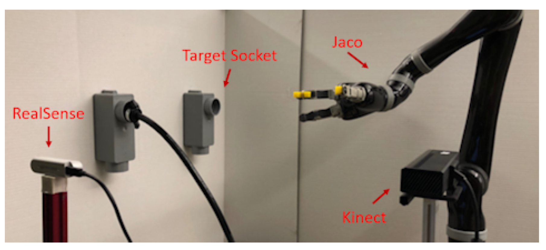
Figure 1. DARPA Robotics Challenge (DRC) Plug Task setup (© 2020 IEEE [29]).
Machines 08 00046 g001
Figure 2. Overall computational model of our system can be represented in an event-driven state machine (© 2020 IEEE [29]).
Machines 08 00046 g002
Figure 3. Steps for obtaining the filtered point cloud (© 2020 IEEE [29]): (left) YOLO object detection, (middle) color detection, (right) point cloud filter.
Machines 08 00046 g003
Figure 4. A modeling example with 10 sample points (© 2020 IEEE [29]).
Machines 08 00046 g004
Figure 5. (left) Cable tip frame, (right) cable frame (© 2020 IEEE [29]).
Machines 08 00046 g005
Figure 6. Cable tip pose alignment (© 2020 IEEE [29])
Machines 08 00046 g006
Figure 7. Simulation environment.
Machines 08 00046 g007
Figure 8. Cable model design.
Machines 08 00046 g008
Figure 9. Simulation-to-Real-to-Simulation (Sim2Real2Sim) flowchart representation.
Machines 08 00046 g009
Figure 10. Cable deformation in Gazebo.
Machines 08 00046 g010
Figure 11. Geometric model in Rviz.
Machines 08 00046 g011
Figure 12. Apriltags attached on the cable for recording the joint values.
Machines 08 00046 g012
Figure 13. Parameters relating three adjacent links. Three links are C i 1 , C i , and C i + 1 . w i is the angular velocity of link C i . m is the mass of the link. L i 1 , i is the vector from the origin of frame i 1 to the origin of frame i. L i 1 , c i is the vector from the origin of frame i 1 to the centre of mass C i . L i , c i is the vector from the origin of frame i to the centre of mass C i . z i is the vector pointing outward and is perpendicular to the paper. f i is the force exerted by link i 1 on link i. τ i is the torque exerted by link i 1 to link i with respect to the origin of the frame i 1 .
Machines 08 00046 g013
Figure 14. Cable model in OpenRAVE.
Machines 08 00046 g014
Figure 15. Updated model with estimated joint stiffness and damping.
Machines 08 00046 g015
Figure 16. From left to right: The robot completing the DRC Plug Task in simulation.
Machines 08 00046 g016
Figure 17. From left to right: The Jaco v2 robot completing the DRC Plug Task in the real world.
Machines 08 00046 g017
Figure 18. From left to right: The Gen3 robot completing the DRC Plug Task in the real world.
Machines 08 00046 g018
Figure 19. Experiment 1: The robot successfully grasps the cable with three different initial states.
Machines 08 00046 g019
Figure 20. Cable modeling with three different initial states.
Machines 08 00046 g020
Figure 21. Experiment 2: Power/HDMI cable pose alignment.
Machines 08 00046 g021
Figure 22. Pose differences between the cable tip frame and the pre-insert frame in Experiment 2.
Machines 08 00046 g022
Figure 23. Experiment 3: (top) Different weights (20 g, 50 g, 100 g) add to the pose alignment control loop as disturbances, (bottom) final pose of the cable after the pose alignment.
Machines 08 00046 g023
Figure 24. Setup in simulation and real world for comparison.
Machines 08 00046 g024
Figure 25. Frames in simulation and real world.
Machines 08 00046 g025
Figure 26. Comparison of the joint positions in simulation and real world (no external force).
Machines 08 00046 g026
Figure 27. Comparison of the joint positions in simulation and real world (a 50 g weight added to the tip).
Machines 08 00046 g027
Figure 28. Comparison of the joint positions in simulation and real world (a 100 g weight added to the tip).
Machines 08 00046 g028
Figure 29. Comparison of the cable deformation between simulation and real world (no external force).
Machines 08 00046 g029
Figure 30. Comparison of the cable deformation between simulation and real world (adding a 50 g weight to the tip).
Machines 08 00046 g030
Figure 31. Comparison of the cable deformation between simulation and real world (adding a 100 g weight to the tip).
Machines 08 00046 g031
Table 1. Estimated model parameters of the power cable for three different initial states.
Poses a 0 a 1 a 2 b 0 b 1 b 2
left−1.882−7.295−5.773−6.041−20.004−15.528
middle−0.385−2.670−2.191−1.917−6.981−5.243
right0.006−1.377−1.125−0.979−3.955−2.806