Abstract
This paper proposes a reliable and straightforward approach to mobile robots (or moving objects in general) indoor tracking, in order to perform a preliminary study on their dynamics. The main features of this approach are its minimal and low-cost setup and a user-friendly interpretation of the data generated by the ArUco library. By using a commonly available camera, such as a smartphone one or a webcam, and at least one marker for each object that has to be tracked, it is possible to estimate the pose of these markers, with respect to a reference conveniently placed in the environment, in order to produce results that are easily interpretable by a user. This paper presents a simple extension to the ArUco library to generate such user-friendly data, and it provides a performance analysis of this application with static and moving objects, using a smartphone camera to highlight the most notable feature of this solution, but also its limitations.
1. Introduction
Recently, the application of mobile robots in indoor environments has increased significantly, mainly due to the technology trends of service robotics and autonomous vehicles. A core technology needed for practically any application related to mobile robots or more generally unmanned vehicles is the localization of the moving agent itself within the environment. From this information, it is then possible to build several typical applications of mobile robots, such as autonomous navigation, multiple agents coordination, mapping, pursuit, and many more. A possible application of the tracking technologies is the study of the dynamic behavior of mobile robots in order to provide further insight. This knowledge can then be used to derive a dynamic model of these systems to develop a proper control architecture, in order to implement autonomous navigation capabilities.
Commercially available solutions addressing this issue are varied and adopt several different technologies. Depending on the particular technology adopted, the tracking system can provide different performances, but generally speaking, if the tracking system is carefully designed, its results are excellent. However, these performances come at a cost to initially set up the system, that may be expensive. Moreover, the setup required to perform the object tracking is highly structured; hence, a suitable space is required. This paper tries to address these two last issues, proposing a low-cost and unstructured solution.
In the next section, an overview of the related tracking technologies is presented. The methods section describes the theoretical methods used to estimate the markers and to evaluate the system performances. After that, the experimental setups required to evaluate the system are illustrated. The experimental results are then presented and discussed. To conclude the paper, the discussion and conclusion sections collect the comments and final remarks about this paper.
Related Research
GPS is the most widely known technology for localization. However, it is limited only to outdoor applications, since in indoor scenarios, it may lack the proper satellite coverage to work correctly, and even if the coverage is enough, its precision is generally inadequate for a mobile agent within an indoor location [1]. For these reasons, different technologies using infrared, light, radio, and ultrasound signals have been developed to overcome the critical issue of localization in indoor scenarios [1,2,3,4]. Generally speaking, these technologies estimate the location following the same working principle [5]: several nodes are located in a scenario composing a network, some of them are in a structured and known location, while the others are fixed to the moving agents to be localized, and signals are sent and received between them. Thanks to some signal properties, such as time of arrival, time of flight, angle of arrival and signal strength, it is possible to measure the distance between the node that has to be located and each of the known ones. Then, performing triangulation from the known distances, it is possible to estimate the location of the node correctly. The main differences in terms of performance and costs between these solutions are mainly due to the kind of signal transmitted between the nodes (Table 1). For example, Wi-Fi based systems are the most common wireless localization systems, simply because most of the node network is already available in many buildings to provide internet connection and it is easy to add new nodes to the system. The main downside is that the signals are generally weak, so to reduce the system inaccuracy, several fixed nodes are required. Lately, ultra wide band (UWB) systems have become one of the most interesting indoor localization technologies based on the use of radio signals [6], mainly due to its high accuracy and some interesting physical features of the short pulses itself, such as obstacle penetration, low noise sensitivity, and high throughput. On the other hand, this technology requires a suitable infrastructure of nodes, that can be expensive to implement to work properly.

Table 1.
Comparison between typical localization technologies.
A different kind of localization system is based on image processing and feature recognition. In these systems, it is possible to estimate the pose of a moving agent processing a video, looking for some particular features to map the 2D image of the frames to the 3D environment. By knowing a priori the dimensions of the features and how the camera transforms points between the image plane and the real environment (the so-called camera model), it is possible to estimate the position and the orientation of the feature and, therefore, of the related agent. What precisely the feature can be, may vary: it can be an easily identifiable moving agent local feature (e.g., SIFT-based systems [7,8]), but, usually, it is a set of artificial markers easily that are recognizable in the scene. Typically, these markers, also known as fiducial markers, are simple geometric figures with bright colors or a black and white pattern encoding a binary matrix. Among the several kinds of fiducial markers proposed in the literature [9,10,11], the square markers are the most widely used, because it is possible to estimate their pose from their four corners (Figure 1). For these reasons, several square fiducial markers have been developed [12,13,14,15], but in this article, ArUco markers [16,17,18] are used, because they were designed for the fast processing of high-quality images and because the core library is open-source [19]. ArUco marker detection uses an adaptive threshold method to increase robustness with different lighting conditions. It also proposes an approach to generate customizable marker sets with high error detection capabilities. ArUco also includes a marker code generation based on mixed integer linear programming, that produces the codes with the highest error detection and correction capabilities in the literature and can even guarantee optimality for small dictionaries.
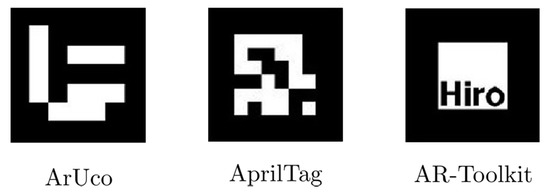
Figure 1.
Examples of square fiducial markers.
Fiducial markers, however, are mainly used in augmented reality applications, or more generally, camera-based systems (i.e., a camera mounted on a robot), so that all the information that can be estimated is available in the camera reference frame. Data represented in this reference frame are not always convenient and easy to understand by a user that desires to track a robot or a vehicle trajectory, in particular if the moving agent is not related at all to the camera. For example, in order to track a mobile robot in a room, it is more useful to estimate the pose about a reference frame fixed to the floor, or, more generally, to the plane of motion of the robot. By doing so, data interpretation by the users is much more immediate and easily interpretable. Moreover, the location of this reference frame could also be a relevant point of interest in the environment itself, so it could be interesting to track a moving agent with respect to (w.r.t. from now on) a relevant point. So, the objective of this study is to develop a system capable of estimating the pose of a robot w.r.t.; a known and convenient reference frame where the trajectory of the robot can be represented intuitively. This approach allows pose estimations to be obtained independently from the camera location, also giving the possibility to let the camera move within the environment while tracking the moving agents. The ArUco core library [19] is used as the starting point, and then it is extended to estimate the pose of the marker w.r.t.; a relevant reference frame instead of the camera one. This article gives a brief introduction about how detection works, then the developed algorithm to localize a moving agent w.r.t.; the desired reference frame is shown. The researchers’ primary objective is not to implement a simple SLAM system, but, instead, a trajectory tracking system able to provide intuitive insight regarding mobile robots’ dynamics for a user, in case a more expensive, structured and sophisticated setup is not available. Some other potential applications of this system are discussed in the discussion section.
The developed system is then tested to evaluate its performance with static and moving markers. In particular, tests are done with a smartphone camera to evaluate the system performance with a minimal and readily available setup, to prove, or not, if a low-cost solution like that can provide a good preliminary trajectory analysis of the moving objects.
Since this paper is an extended version of [20], it provides further insights regarding both the theoretical and experimental parts. Moreover, the system is evaluated with an actual mobile robot performing some trajectories.
This research topic has been developed to track robotic platforms with a setup adaptable to various fields of application, such as a precision agriculture UGV [21], a search and rescue UGV [22], or a stair-climbing wheelchair [23].
2. Materials and Methods
In this section, the original ArUco markers’ localization algorithm developed in [16,18,19] is briefly introduced and explained; then, the developed feature that enables the estimation of the pose of a marker w.r.t., the desired reference frame, is illustrated. At the end of the theoretical analysis, the experimental setups used to evaluate the developed system are presented.
2.1. Methods
The ArUco library can generate a calibration board that is, as shown in Figure 2, a chessboard composed of black squares and square markers. Thanks to this board, it is possible to perform the camera calibration to obtain all the required parameters, to perform a geometric transformation between the image plane of the camera to the actual environment, and vice versa. The calibration process is relatively straightforward: many pictures of the calibration board are taken with different perspectives, trying to cover all the possible scenarios the camera could be placed. It is important to note that the camera settings (mainly its lenses and its focus setting) must always be the same, and the same camera settings must be used during the following pose estimation process. By post-processing all of the pictures collected with the ArUco library, it is possible to get the camera parameters.
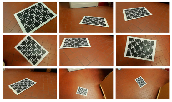
Figure 2.
Camera calibration process. The camera takes several pictures of the calibration board from different perspectives. By Post-processing all these images, it is possible to get the camera calibration parameters.
When the camera calibration is completed, the marker localization process begins. The process, visually represented in Figure 3, is commonly used in computer vision applications, with some minimal variations depending on the particular algorithms adopted. First of all, an image is opened (a); it can be a still image, or it can be a frame extracted from a video, and it is converted in a grayscale picture to improve the results of the next step, the adaptive thresholding process (b). At this point, all the contours, or at least all the contours related to a sufficient change of color, should be available; however, all the contours that are not closed and approximated by four sides are filtered out by a contour detection algorithm (c). All the remaining contours may form a square marker, so for each of them, it is done a process of perspective removal (d) and a binary code encoding (e), to verify if the contour is a marker or not. The binary encoding step consists of converting the unique pattern of black and white squares into a binary matrix of zeros (for the black squares) and ones (for the white ones) that encode the unique marker ID. If a marker is identified, its ID and its four corners’ coordinates in the image plane are stored. When all the possible candidates have been checked, the sequence is completed. The whole process is summarized in Algorithm 1.
| Algorithm 1: Automatic marker detection and localization algorithm | |||
| whileFrame of the video is availabledo | |||
| begin Automatic Markers Detection Process | |||
| Get frame from video; | |||
| Convert frame to grayscale; | |||
| Apply adaptive thresholding to frame; | |||
| Find contours; | |||
| Remove contours with low number of points; | |||
| Approximation of contours to rectangles; | |||
| Remove rectangles too close | |||
| Remove prospective to get frontal view | |||
| Apply Otsu’s threshold algorithm | |||
| Identify marker from its binary code; | |||
| ifmarker is identifiedthen | |||
| Refine corners; | |||
| end | |||
| Provide list of corners and IDs; | |||
| end | |||
| begin Marker Pose Estimation Process | |||
| Foreach IDdo | |||
| Apply transformation from 2D to 3D to corners; | |||
| Produce list of poses w.r.t. camera; | |||
| end | |||
| end | |||
| end | |||
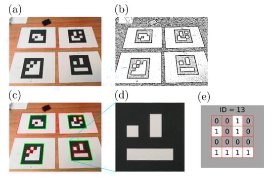
Figure 3.
Marker detection process. (a) Original frame. (b) Results of thresholding. (c) Contours detection; in green, the squares that will be identified as markers are shown, in red, instead, all the rejected squares. (d) Prospective removal. (e) Identification from binary.
When at least one marker has been identified, it is possible to estimate its pose thanks to the camera parameters obtained by the calibration process. These parameters define the pinhole camera model required to perform the geometric transformation between the projected image plane and the actual 3D environment (Figure 4). A simple pinhole camera model can be represented as follows:
where and are the 2D image coordinates,, and are the 3D camera coordinates, is the intrinsic matrix of the camera composed by some parameters obtained by the camera calibration, such as , (the focal lengths), and (the origin of the image plane), and (the skew factor). The camera calibration process also provides some distortion factors to compensate for the lens distortion.
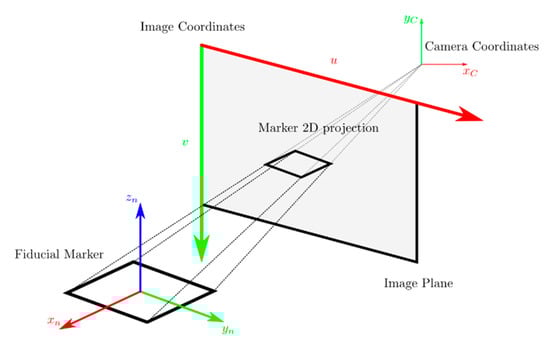
Figure 4.
Pinhole camera model applied to a single square marker. The camera model allows the image projection to be represented in the 3D environment, or vice-versa.
At this point, from the known 3D coordinates of the four corners, it is trivial to get the center of the square marker and its orientation, carrying out the pose estimation w.r.t.; the camera reference frame. To introduce some notation that is used in this article, from now on, the pose of a generic point in the reference frame is represented as follows
where the homogeneous transformation contains the rotation matrix and the translation vector needed to represent a generic reference frame or point in a reference frame .
All these operations are repeated for each marker identified in the previous steps, then a new video frame is loaded, and the algorithm is repeated until the last frame.
At this stage, all the homogeneous transformations , with , between the camera and all the identified markers are known. While these kinds of data can be useful and convenient for augmented reality or camera-centered applications, or more generally, for an algorithm, they are not so intuitive for a human user whose task is to track one or more mobile agents in order to study their trajectories. For this reason, an additional step to the core functionalities has been developed, with the intent to represent these poses w.r.t.; a convenient reference frame that can be physically placed where required, for example, in a relevant point of the plane of motion, so the user has a physical reference in the environment to which it is more intuitive to associate the trajectories of the moving objects.
As a convention defined here, this reference frame is represented by the ArUco marker with and it will be referenced as the “fixed reference frame,” even if it does not need to be static. Therefore, from the previous algorithm, it is possible to estimate the pose of this marker w.r.t. the camera reference frame , then applying the matrix inversion , the pose of the camera w.r.t.; the fixed reference frame is now known. So, in the end, it is possible to represent the pose of the nth marker w.r.t.; the reference one by a concatenation of homogeneous transformation (as represented in Figure 5 and described in Algorithm 2).
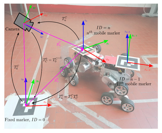
Figure 5.
Graphical representation of the relations between reference frames of the camera, the fixed reference and the generic nth marker and the corresponding homogeneous transformations.
| Algorithm 2: Improved Automatic marker detection and localization algorithm | ||||
| whileFrame of the video is availabledo | ||||
| begin Automatic Markers Detection Process | ||||
| Same as in Algorithm 1 | ||||
| end | ||||
| begin Improved Marker Pose Estimation Process | ||||
| foreach IDdo | ||||
| Apply transformation from 2D to 3D to corners; | ||||
| Produce list of poses w.r.t. camera; | ||||
| Reorder list | ||||
| ifID equal to 0then | ||||
| Compute | ||||
| else | ||||
| Compute | ||||
| end | ||||
| end | ||||
| Produce list of poses w.r.t. reference frame; | ||||
| end | ||||
| end | ||||
In particular, the position of the center of the nth marker is the translation vector , while its orientation can be derived by the rotation matrix and both these components can be obtained from the homogeneous transformation matrix . For the sake of completeness, during most of the execution of the algorithm and in the data logging, rotations are not represented by a rotation matrix, but by a rotation vector in the axis-rotation form to get more algorithm-efficient data. So, the generic rotation vector represents a rotation of an angle about an axis and it is related to the generic rotation matrix by these relations:
At this point, more natural results for a user are obtained, since the fixed marker acting, both conceptually and physically, as a reference frame could be placed where it is convenient and meaningful to represent the poses of the other markers fixed to the actual moving objects. By doing so, it is possible to achieve the required feature of estimating a trajectory w.r.t.; the desired frame in order to perform the required vehicle dynamics analysis. It is also relevant to state that the pose estimations could happen both in real-time, using a live video stream, and offline, processing a pre-recorded video.
Extending this concept, now the pose data are no more related to the camera location in the environment, so the camera may even move while recording the scene, but the system would still be able to estimate the pose correctly. However, it is essential to note a limitation of this last feature: to estimate the pose of a marker w.r.t. the fixed reference, the algorithm must identify both of them as markers, so they must appear in the frames recorded by the camera. If this condition is not satisfied, the algorithm cannot compute the inversion of homogeneous transformation and the successive concatenation of transformations.
Going even further, as briefly hinted before, it is also possible that the fixed reference frame is not fixed at all, and it can move around like all the other markers. This particular scenario can be useful when it is required to know the pose of an object w.r.t. a moving one, like in applications such as platooning, robot swarm, or agent pursuit. In these scenarios, it is even more critical that the camera sees all the markers, so letting the camera move around, maybe mounted on a flying drone, could be convenient in some scenarios.
Some quantities must be defined to evaluate system performances. Given the nth marker, several of its pose estimations are available if it is static (in the best scenario, there is an estimate for each frame of the video), so it is possible to define and compute the mean position and the relative standard deviation as follows, where is the number of collected samples.
In order to evaluate the correlation of distance from the camera and uncertainty, some additional parameters are defined. Moreover, these parameters are normalized using the marker side length to compare the results of all the tests fairly. The distance between the camera and the marker nth marker and the associated normalized parameters are defined as
As a side note, the norm of the relative position and the norm of standard deviation vector are used to condense the information in two scalar parameters, but it is also possible to perform a similar analysis using the vectors instead.
2.2. Experimental Setup
After this brief introduction about the methods used behind this study, the main elements of the experimental setup are presented. The first of the main elements is the camera: any camera could work, but to stay true to the readily available setup requirement, in this study, a typical smartphone camera, without additional lenses, is used. Such camera records video with a resolution of 1080p at 30 FPS. The camera has 12MP, an f/2.2 aperture, a sensor size of , and pixel size of . A USB webcam was also tested, but since its first results were mediocre, it was not used. As shown before, whichever camera is used, the calibration phase has to be done to get the camera parameters.
The second element required is a set of fiducial markers. In this system, ArUco markers are used. In particular, the 4x4 ArUco dictionary (another name for the set of markers, where the dimensions are the number of squares used to encode the marker ID) has been used to generate all the required markers. The adopted dictionary has little impact on the system itself: it is possible to get a higher number of unique IDs increasing the number of squares. This, however, comes at the cost of smaller squares in the binary pattern given the same overall size. 16 unique markers have been generated with the ID ranging from 0 to 15, with marker side length of 48 mm or 96 mm to perform the experimental evaluation of the system. Again, the exact ID value does not matter; it is simply necessary that all of the markers in the scene are unique, and that among them there is the reference one, that, as an arbitrary convention, is the maker with . Also, the exact number of markers does not matter; the actual limit is the number of unique markers that the dictionary can generate.
In the static tests, the markers are simply fixed to the floor, trying to cover the whole area that the camera can see (Figure 6). For a couple of static experimental setups, the markers are placed in a grid of known (measured) dimensions to evaluate the system accuracy; in other cases, the markers are placed randomly, trying to cover the whole camera field of view instead. A video records the scene for about 10 s, so it is possible to collect up to 300 estimations per marker during the whole sequence. After a recording is complete, the markers can be shuffled around, the camera can be moved in another position, or its height from the floor can be changed, and then a new test can be done.
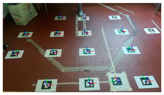
Figure 6.
Setup to evaluate the static performance of the system. This picture also shows that the algorithm places a reference frame at each identified marker center, while the unidentified ones remain without axes.
A remotely controlled robot is used to have some markers moving in a controllable way. The robot prototype, called Epi.q mod2 (Figure 7), is the last model of a unique family of mobile robots [24]. It is a modular robot composed of two almost identical modules (front and rear), that are linked together by a passive joint that enables relative roll and yaw movements between modules. The most important feature of this robot is its unique locomotion units that dynamically mix wheeled and legged locomotion [25], in order to overcome little obstacles. Two markers are fixed on the robot chassis, one for each module, to test the tracking system with moving objects, while the fixed reference marker is fixed on the floor where the robot moves. The robot is controlled to follow simple trajectories (e.g., straight and circular trajectories) defined by an internal code, or it can be directly controlled by a user with a remote controller to perform more complex maneuvers. Each robot module can be controlled as a differential drive robot; however, during these tests, only the front module is actuated, while the rear module is being pulled like a trailer. It is essential to highlight that, at the moment, there is no communication between the robot and the tracking system, so the two are independent. It may be possible, however, that in the future, the marker localization system could be improved and integrated with a mobile robot, to allow autonomous navigation in indoor scenarios.
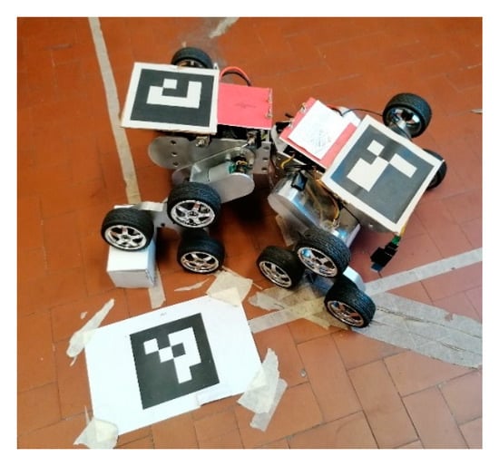
Figure 7.
Epi.q mod2, the remotely controlled mobile robot used for testing the localization system with moving markers while climbing a little obstacle. The markers with ID 1 and 2 are fixed respectively on the front (left in the photo) and rear (right) module. The fixed reference (Marker ID 0) is fixed to the floor instead.
3. Results
In this section, the results of the experimental tests to evaluate the performance of the proposed tracking system are presented. In the first part, the tests with static markers are discussed, while in the second part, the tests with moving markers are presented.
3.1. Static Markers
Table 2 collects the results of a test done with eight static markers, with accurately placed w.r.t. the reference marker, as shown in the first column. The results show that each marker average estimate is always within from the true value, a relatively good result compared to the marker size and to the possibility of tracking a moving robot. The uncertainty is limited too, but it is already noticeable an issue that is addressed in the next paragraphs.
Table 2.
Static test results: accuracy and uncertainty.
In Figure 8, it is possible to see the results of one of the many tests with a marker size of . The results are so good that the marker estimations distribution is hidden by the size of the points used to represent them, in particular for markers closer to the camera.
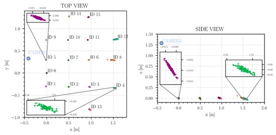
Figure 8.
Results of the localization algorithm. Marker side length of 96mm. For the marker closest to the camera, the actual point distributions are significantly smaller than the points used in the pictures.
The most remarkable test results aspect is that the point distribution relative to each marker lies along the line connecting the mean position of the marker and the camera position: this outcome is linked to the typical difficulties of estimating depth from a single camera. This issue is particularly evident in the XZ plane, because the minimum vertical distance for all the markers is always above 1.25 m (the camera height from the floor), so each marker always has a substantial uncertainty in the XZ plane. In contrast, in the XY plane, this effect is more apparent for markers farther away from the camera, so it is possible to state that this effect is due to the distance from the camera, or in other words, because of the well-known problem of measuring the depth from a single camera. This outcome is not a surprise, as it is a typical problem of single-camera image-based systems, and the common way to solve it could be a new experimental configuration with a stereo-camera, or with at least two cameras with known relative positions. These solutions allow the uncertainty to be noticeably reduced by fixing the depth estimation issue, but they also increase the setup costs, and in the case where several cameras are needed, the environment needs to be highly structured to support the system.
From these results, it is possible to state that the position of the markers is estimated where expected and the precision is higher for the markers closer to the camera ( around 0.5 mm), and it decreases a little when the marker is further away ( up to 5 mm, some outliers goes up to 20 mm). Slightly worse results are obtained with markers with a smaller side length (48 mm).
Even if the marker pose is represented in the desired frame independently from the camera position, the results show that the estimation uncertainty is related to the relative position of the camera and the markers, in particular the distance between them. In Figure 9, it can be easily seen that the normalized uncertainty increases when the normalized distance increases, and in particular, it can be stated that a parabolic function relates precision and distance. From this image, it is also possible to prove the claim that better precision can be achieved with larger markers, while a slightly worse precision can be achieved if smaller markers are used. An alternative interpretation of these data is that the smaller markers can be seen as markers with the same size as the other, but “virtually” further away from the camera.
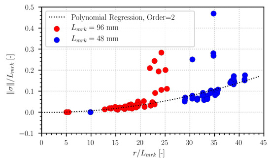
Figure 9.
Localization accuracy as a function of distance from the camera. Values are normalized using the marker side length.
Many characteristics of the established tracking method can already be derived from the results of the tests with static markers. Even if the markers’ poses are represented in the desired fixed reference frame, regardless of the camera position, the distance is still relevant as a parabolic function relates it to the uncertainty . The camera position is therefore key to obtain the optimal results in terms of precision, and the system setup has to be set accordingly, minimizing the relative distance between the camera and the markers. An experimental setup with a moving camera may help in this process, as it can reduce the distances as required or when it is needed, but if the camera moves too quickly, it is also possible to introduce motion blur. In the next part, this last problem is discussed in more detail, as it can also occur when the camera is static, and the markers are moving, or both are moving.
The angle between the marker plane and the relative distance vector also plays a role in the marker detection ability. If this angle is relatively small, perspective distorts the marker projection on the object plane, and the marker cannot be detected if the distortion is significant; however, there was no measuring instrument accurate enough to provide further insights. Nevertheless, qualitatively speaking, the range of angles from which the markers can still be tracked is compatible with most of the setups where a camera is capturing the environment from the top.
From these initial observations, it is clear that the parameters of the camera and its position are essential to a successful localization process. However, it may be possible to achieve slight performance improvements at the cost of higher expenses and complexity. First of all, the results shown here proved that a larger marker guarantees better precision, so it is advisable to use the largest marker possible. Another interesting solution might be to fix more than one marker to the object to be tracked, in order to perform a kind of data fusion approach. In doing so, some uncertainty can be filtered out, and some partial occlusion cases can also be overcome too: if at least one of the multiple markers is detected, its pose can be estimated. Further along this path, several cameras and several markers for the single object could be used to enforce a proper approach to data fusion and a proper setup capable of setting up camera occlusion scenarios. However, it is clear that going further in these directions, the initial requirement of a low-cost and readily available experimental setup to track some markers is lost.
3.2. Moving Markers
Two main issues need to be addressed when a moving marker has to be tracked. First, if the marker moves above a specific speed limit, or if the relative speed between the marker and the camera is too high, the video frame may become blurred, making it impossible to obtain an image with well-defined contours required to detect or identify the marker successfully during its movement. Referring to the previous part about how the markers tracking works, it is possible that, while moving, the marker may be detected as a potential marker, but its binary pattern is so blurred that its encoding process, and therefore the marker identification, fails. It is also possible, if the marker moves even faster, that the marker is not detected at all, and the identification phase is skipped. The latter possibility is generally more related to a marker moving far away from the camera rather than its actual speed in doing so. It may be possible to fail the marker detection phase if the marker in the image frame is so distorted that a convex four-sided polygon does not approximates it anymore. It is more common that this situation is due to a very distorted perspective than a fast-moving marker. Second, a moving marker, due to the perspective, can become virtually larger or smaller in the image frame if it moves closer or further away from the camera. So, while it moves closer to the camera, the localization results are generally better, but when the marker moves away, the uncertainty increases. It is also possible that the marker moves so far away that it becomes so small in the picture, that it is not possible to detect the marker anymore, or, as said before, it becomes so distorted by the perspective that it is impossible to detect the marker.
From the experimental evidence, it appears that the transformations between the 2D image projection and the actual environment have a significant influence in analyzing the dynamic system performances. Going further, it appears that perspective plays a major role in this. In Figure 10, horizontal and vertical displacements that take place in the 3D environment and that are projected on the image plane are represented. By focusing on the horizontal displacements in the figure, it appears that different equalities hold depending on which references are seen: in the 3D environment , while is a larger displacement, but in the image plane the equality holds, while is a shorter movement. In other words, two points moving at the same speed, but a different distance from the camera, appears to be moving at different speeds in the image plane, while two points moving at different speeds may appear to be moving at the same speeds in the image plane. This issue is also present, if not even more evident, for the vertical displacements.
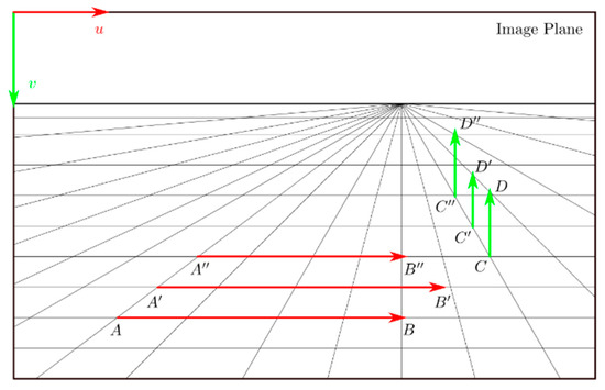
Figure 10.
Graphical representation of the issue of representing speeds in the image plane or in the 3D environment. In the image plane, the following relations are true and , while in the actual environment and are true instead.
Since the detection and identification of the actual markers seems to be strongly related to the image plane, in this article, the dynamic analysis of the system is done in the image plane using speeds measured in pixel per frame in the image space along the and axis. However, it is possible to perform a similar analysis in the real 3D environment if the camera model is known.
Figure 11 depicts how the extended algorithm can measure the speed of an object in the image space. At the beginning, the center of the fiducial marker is projected to the image plane and its position is estimated in pixels unit. After some time , the object gets detected and projected again. Hence, it is possible to compute the position difference between the two frames . The velocity in pixel/frame is obtained by dividing this variation by the frames increment.
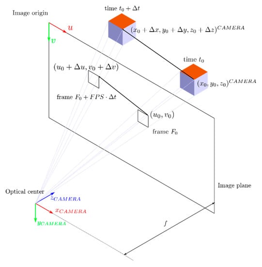
Figure 11.
Working principle of the pinhole camera model applied to a moving object.
The dynamic tests consist of the camera recording several trials where the robot moves from a still position to a reference speed in straight horizontal and vertical lines. Figure 12 shows how often a moving marker is identified while moving at a particular speed: a still marker is always detected and identified, while, for faster moving markers, the detection probability decreases. The detection probability becomes almost zero when a marker is moving with a horizontal over and a vertical speed over . As said before, the transformation matrix between the 3D world and its 2D projection is required to relate these values to the actual speed of the robot, since they can represent different speeds depending on the perspective. It also appears that the results in the vertical direction are slightly worse than the one in the horizontal direction. The most probable explanation is that while the robot moves horizontally, it stays about the same distance from the camera during its path, but if the robot moves vertically, it moves further away from the camera, worsening the localization results.
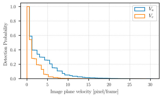
Figure 12.
Horizontal and vertical speeds detection rate in the image plane.
It should be possible to increase the number of analyzed frames increasing the camera FPS, improving the possibility to detect the markers, but also giving the possibility to collect more data enabling some filtering to estimate the missing estimation as well. Common camera sensors from a smartphone or a webcam can generally reach up to 60 FPS at the cost of image quality. High-end commercial camera sensors instead can reach 60 FPS without compromising the image quality. High-speed cameras would be the best solution, but with such instruments, the requirement to have a low-cost and readily available setup is lost.
A possible solution to the problem related to the image perspective could be trying to get the image plane as parallel as possible to the plane of motion of the markers; i.e., a top view of a simple planar motion. In this way, the depth has little if no effect, so the speeds are easily relatable. Regarding the relative camera-marker distance, it appears that centering the markers close to the camera optical axis reduces distortion effects that are evident when close to the border of the image.
The issues of detecting markers under challenging conditions such as inadequate lighting or high blur due to fast motion are very common while using this type of markers, that have been developed mainly for static or semi-static applications, like augmented reality. The trend to overcome these kinds of issues seems to avoid the identification of the marker by encoding a possible pattern of a closed region in favor of an identification based on machine learning classification [26]. The bits extraction steps to encode the marker require that the pattern is easily recognizable; however, it is not always possible if a lot of motion blur, or other conditions such as defocus, non-uniform lighting or small size, applies. For this reason, a classifier is trained with several labeled pictures of markers in different conditions, to identify the markers using a neural network instead. This leads to a more robust system, but the cost is a more computational heavy algorithm that may not work in real-time if there is a high number of markers. Moreover, the machine learning approach requires accurate algorithm training in order to work, even in static conditions.
3.3. Robot Trajectory
This section briefly shows the application of the localization algorithm that leads to the development of this tool: vehicle dynamics tracking of a mobile robot. The experimental data collected with the tracking system are then compared with a simulated dynamic model of the robot. The dynamic model is derived and described in [27]. The model is a planar dynamic model of modular articulated robots like Epi.Q. Due to the robot locomotion unit architecture, the model implements wheel-ground contact forces that take into account wheel slippage and skidding. The parameters required to simulate the model have been obtained through an experimental identification.
As before, Epi.q mobile robot with the two markers is used as a moving agent. Two pre-defined speed profiles are used as references for the left and right motors to obtain repeatable trajectories. The remote controller acts just like a remote power switch, without any other control of the robot. The most common maneuver that can provide useful vehicle dynamics insight, excluding the trivial straight path, is the circular one. The robot starts from a still position and accelerates to reach the steady-state condition; then, applying a higher velocity to one of the motors, the robot performs a circular trajectory with a constant curvature radius. Figure 13 presents the comparison between the filtered collected data and a dynamic simulation with the same initial conditions and inputs. The two trajectories are comparable, and the main difference between them seems, in particular, to be referencing the actual video recording, due to non-simulated dynamics effects. The robot locomotion units are subject to considerable wheel slippage, since all the wheels of the same units spin at the same speed, due to the employed gearing system. This effect is even more evident when lateral dynamics are considered. Given that these wheel dynamics are only partially implemented in the simulated model, and that the tracking system results shown before are sufficiently accurate and precise, it is supposed that the main source of divergence between the experimental data and the simulation is due to unmodelled dynamics, that with high probability, are related to the dynamics of the wheels. Nevertheless, it is possible to say that the tracking system can provide initial insights to begin the study of mobile robot dynamics using a minimal setup, achieving the intentions that lead to this study. It is clear that a proper tracking setup could, with high probability, overperform this system; however, it cannot be denied that, with the proposed tool, it is possible to collect data without any dedicated instruments with sufficient accuracy, to derive some useful information from the experimental data.
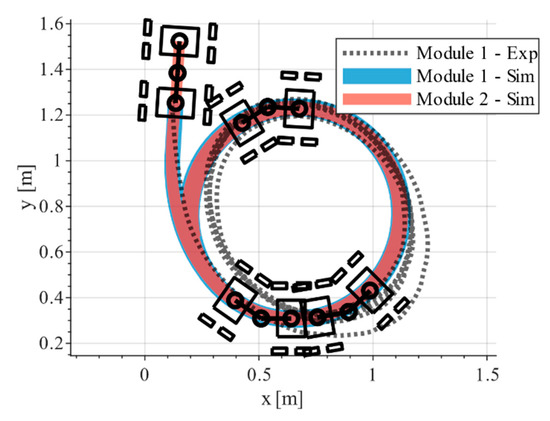
Figure 13.
Position estimation of markers 1 and 2 fixed to a robot performing a circular trajectory. It is possible to note that two shifted circles appear, due to wheels slippage and other dynamic effects.
4. Discussion
This article showed an extended fiducial marker tracking algorithm based on the ArUco library that can track a mobile robot indoors, allowing the user to estimate the location of the markers in the desired reference frame, enabling a more intuitive data representation for the user. Moreover, the performances of this tool have been tested positively, using a smartphone camera to verify if the whole setup could provide significant results to derive insight about the robot dynamics without the need of a commercial tracking setup, but using only a readily available instrument (the smartphone camera) and with minimal overall cost.
With markers with a side length of 96 mm, it is possible to estimate their location with a precision of less than 1 cm within a distance of 3 m from the camera, using a low cost and easy to use configuration. At the same time, the tracking system can obtain an accuracy that is less than 6 mm within a distance from the camera 1.5 m. It is possible to achieve even better precision and improved coverage increasing the size of the markers. Results from tests with different camera-marker distances show the relationship between camera precision and range: the lower the distance, the better the precision. Therefore, the established localization method can provide a location estimation that is accurate enough to be used in relatively small rooms. These results also fall within the expected ranges of similar systems based on image processing, but with the additional feature of more intuitive estimate representation. However, the adopted monocular camera setup leads to an inevitable issue related to depth estimation; therefore, comparable setups with more than one camera perform better than the proposed solution, in particular at longer ranges. It is planned to compare this system’s performance directly with a more sophisticated system in the future.
If more accuracy or range is needed, the camera sensor can be improved; the camera position can be modified to reduce the camera-marker distances, the size of the markers can be increased to make them appear “virtually” closer to the camera, the single object can be tracked using several markers fixed to it to implement a data fusion approach (probably the best approach, in the sense that it fixes three makers onto three different surfaces, perpendicular between them). The latter solution can also help in case of partial occlusion of the object.
The dynamic experiments have revealed that this method of position estimation is still robust and reliable when the markers move in the environment. The camera was able to detect movements of within ±20 pixel/frame in the horizontal direction and within ±10 pixel/frame in the vertical direction. Higher velocities were also observed and detected (in the horizontal direction in particular), but with significantly lower confidence. It is highly probable that a camera with a higher frame rate and an even better resolution may obtain even better results. However, further analysis will be required to understand better how the system behaves.
5. Conclusions
To conclude, this system can work as a marker tracking system enabling markers pose estimation w.r.t. an intuitive reference frame, in order to perform some trajectory analysis. In addition, this system can work using a readily available camera, such as a smartphone camera, and still provide significant results in contained environments. So, it is possible to conclude that this tool achieved the two requirements that led to its development: a readily available and low-cost setup that could enable any researcher to perform some trajectory analysis, even without a proper experimental setup.
By adding some kind of communication between this system and the robot, this localization algorithm could be used in real-time to send data to the robot, in order to achieve some kind of autonomous navigation capability where the relative motion w.r.t; a given reference is required.
Author Contributions
Funding acquisition, G.Q.; Methodology, A.B.; Project administration, G.Q.; Software, A.B.; Supervision, G.Q.; Writing—original draft, A.B.; Writing—review & editing, A.B. and G.Q. All authors have read and agreed to the published version of the manuscript.
Funding
This research received no external funding.
Conflicts of Interest
The authors declare no conflict of interest.
References
- Torres-Solis, J.; Falk, T.H.; Chau, T. A Review of Indoor Localization Technologies: Towards Navigational Assistance for Topographical Disorientation. Ambient Intell. 2010. [Google Scholar] [CrossRef]
- Dhobale, M.D.; Verma, P.S.; Joshi, P.R.; Tekade, J.K.; Raut, S. A Review on Indoor Navigation Systems and Technologies for Guiding the Users. Int. J. Sci. Res. Comput. Sci. Eng. Inf. Technol. (IJSRCSEIT) 2019, 5, 244–250. [Google Scholar]
- Ijaz, F.; Yang, H.K.; Ahmad, A.W.; Lee, C. Indoor positioning: A review of indoor ultrasonic positioning systems. In Proceedings of the 2013 15th International Conference on Advanced Communications Technology (ICACT), PyeongChang, Korea, 27–30 January 2013; pp. 1146–1150. [Google Scholar]
- Sanpechuda, T.; Kovavisaruch, L. A review of RFID localization: Applications and techniques. In Proceedings of the 2008 5th International Conference on Electrical Engineering/Electronics, Computer, Telecommunications and Information Technology, Krabi, Thailand, 14–17 May 2008; Volume 2, pp. 769–772. [Google Scholar]
- Mozamir, M.S.; Bakar, R.B.A.; Din, W.I.S.W. Indoor Localization Estimation Techniques in Wireless Sensor Network: A Review. In Proceedings of the 2018 IEEE International Conference on Automatic Control and Intelligent Systems (I2CACIS), Shah Alam, Malaysia, 20–20 October 2018; pp. 148–154. [Google Scholar]
- Alarifi, A.; Al-Salman, A.; Alsaleh, M.; Alnafessah, A.; Al-Hadhrami, S.; Al-Ammar, M.A.; Al-Khalifa, H.S. Ultra wideband indoor positioning technologies: Analysis and recent advances. Sensors 2016, 16, 707. [Google Scholar] [CrossRef] [PubMed]
- Se, S.; Lowe, D.; Little, J. Mobile robot localization and mapping with uncertainty using scale-invariant visual landmarks. Int. J. Robot. Res. 2002, 21, 735–758. [Google Scholar] [CrossRef]
- Se, S.; Lowe, D.; Little, J. Vision-based mobile robot localization and mapping using scale-invariant features. In Proceedings of the 2001 ICRA. IEEE International Conference on Robotics and Automation (Cat. No. 01CH37164), Seoul, South Korea, 21–26 May 2001; Volume 2, pp. 2051–2058. [Google Scholar]
- Kato, H.; Billinghurst, M. Marker tracking and HMD calibration for a video-based augmented reality conferencing system. In Proceedings of the 2nd IEEE and ACM International Workshop on Augmented Reality (IWAR’99), San Francisco, CA, USA, 20–21 October 1999; pp. 85–94. [Google Scholar]
- Fiala, M. Designing Highly Reliable Fiducial Markers. IEEE Trans. Pattern Anal. Mach. Intell. 2010, 32, 1317–1324. [Google Scholar] [CrossRef] [PubMed]
- Schmalstieg, D.; Fuhrmann, A.; Hesina, G.; Szalavári, Z.; Encarnação, L.M.; Gervautz, M.; Purgathofer, W. The Studierstube Augmented Reality Project. Presence Teleoperators Virtual Environ. 2002, 11, 33–54. [Google Scholar] [CrossRef]
- Da Neto, V.F.C.; de Mesquita, D.B.; Garcia, R.F.; Campos, M.F.M. On the Design and Evaluation of a Precise Scalable Fiducial Marker Framework. In Proceedings of the 2010 23rd SIBGRAPI Conference on Graphics, Patterns and Images, Gramado, Brazil, 30 August–3 September 2010; pp. 216–223. [Google Scholar]
- Atcheson, B.; Heide, F.; Heidrich, W. Caltag: High precision fiducial markers for camera calibration. In VMV 2010—Vision, Modeling and Visualization; VMW: Siegen, Germany, 2010; Volume 10, pp. 41–48. [Google Scholar]
- Olson, E. AprilTag: A robust and flexible visual fiducial system. In Proceedings of the 2011 IEEE International Conference on Robotics and Automation, Shanghai, China, 9–13 May 2011; pp. 3400–3407. [Google Scholar]
- DeGol, J.; Bretl, T.; Hoiem, D. ChromaTag: A Colored Marker and Fast Detection Algorithm. In Proceedings of the 2017 IEEE International Conference on Computer Vision (ICCV), Venice, Italy, 22–29 October 2017; pp. 1481–1490. [Google Scholar]
- Garrido-Jurado, S.; Muñoz-Salinas, R.; Madrid-Cuevas, F.J.; Marín-Jiménez, M.J. Automatic generation and detection of highly reliable fiducial markers under occlusion. Pattern Recognit. 2014, 47, 2280–2292. [Google Scholar] [CrossRef]
- Garrido-Jurado, S.; Muñoz-Salinas, R.; Madrid-Cuevas, F.J.; Medina-Carnicer, R. Generation of fiducial marker dictionaries using Mixed Integer Linear Programming. Pattern Recognit. 2016, 51, 481–491. [Google Scholar] [CrossRef]
- Romero-Ramirez, F.J.; Muñoz-Salinas, R.; Medina-Carnicer, R. Speeded up detection of squared fiducial markers. Image Vis. Comput. 2018, 76, 38–47. [Google Scholar] [CrossRef]
- Munoz-Salinas, R. ARUCO: A Minimal Library for Augmented Reality Applications Based on OpenCv; Universidad de Córdoba, 2012; Available online: https://www.uco.es/investiga/grupos/ava/node/26 (accessed on 30 May 2020).
- Botta, A.; Quaglia, G. Low-Cost Localization For Mobile Robot With Fiducial Markers. In Proceedings of the 25th Chiefdom Symposium (2019) 2nd International Jc-IFToMM Symposium, Kanagawa, Japan, 26 October 2019. [Google Scholar]
- Quaglia, G.; Cavallone, P.; Visconte, C. Agri_q: Agriculture UGV for Monitoring and Drone Landing. In Mechanism Design for Robotics, Proceedings of the Mechanism Design for Robotics, held in Udine, Italy, 11–13 September 2018; Gasparetto, A., Ceccarelli, M., Eds.; Springer International Publishing: Cham, Switzerland, 2019; pp. 413–423. [Google Scholar]
- Quaglia, G.; Cavallone, P. Rese_Q: UGV for Rescue Tasks Functional Design; American Society of Mechanical Engineers Digital Collection: Pittsburgh, PA, USA, 2019. [Google Scholar]
- Quaglia, G.; Nisi, M. Design and Construction of a New Version of the Epi.q UGV for Monitoring and Surveillance Tasks; American Society of Mechanical Engineers Digital Collection: Houston, TX, USA, 2016. [Google Scholar]
- Bruzzone, L.; Quaglia, G. Locomotion systems for ground mobile robots in unstructured environments. Mech. Sci. 2012, 3, 49–62. [Google Scholar] [CrossRef]
- Mondéjar-Guerra, V.; Garrido-Jurado, S.; Muñoz-Salinas, R.; Marín-Jiménez, M.J.; Medina-Carnicer, R. Robust identification of fiducial markers in challenging conditions. Expert Syst. Appl. 2018, 93, 336–345. [Google Scholar] [CrossRef]
- Brena, R.F.; García-Vázquez, J.P.; Galván-Tejada, C.E.; Muñoz-Rodriguez, D.; Vargas-Rosales, C.; Fangmeyer, J. Evolution of indoor positioning technologies: A survey. J. Sens. 2017, 2017, 21. [Google Scholar] [CrossRef]
- Botta, A.; Cavallone, P.; Carbonari, L.; Tagliavini, L.; Quaglia, G. Modelling and experimental validation of articulated mobile robots with hybrid locomotion system. In Proceedings of the 3rd IFToMM ITALY Conference, Naples, Italy, 9–11 September 2020. Accepted. [Google Scholar]


© 2020 by the authors. Licensee MDPI, Basel, Switzerland. This article is an open access article distributed under the terms and conditions of the Creative Commons Attribution (CC BY) license (http://creativecommons.org/licenses/by/4.0/).