Simulation of Subcritical Vibrations of a Large Flexible Rotor with Varying Spherical Roller Bearing Clearance and Roundness Profiles

Abstract

In large rotor-bearing systems, the rolling element bearings act as a considerable source of subcritical vibration excitation. Simulation of such rotor bearing systems contains major sources of uncertainty contributing to the excitation, namely the roundness profile of the bearing inner ring and the clearance of the bearing. In the present study, a simulation approach was prepared to investigate carefully the effect of varying roundness profile and clearance on the subcritical vibration excitation. The FEM-based rotor-bearing system simulation model included a detailed description of the bearings and asymmetricity of the rotor. The simulation results were compared to measured responses for validation. The results suggest that the simulation model was able to capture the response of the rotor within a reasonable accuracy compared to the measured responses. The bearing clearance was observed to have a major effect on the subcritical resonance response amplitudes. In addition, the simulation model confirmed that the resonances of the 3rd and 4th harmonic vibration components in addition to the well-known 2nd harmonic resonance (half-critical resonance) can be significantly high and should thus be taken into account already in the design phase of large subcritical rotors.

1. Introduction

Large rotor-bearing systems are commonly used in the industry as a part of, e.g., electric motors and generators, turbines in renewable or fossil energy production, and paper, steel and non-ferrous metal manufacturing machinery. The rolling element bearings act as a considerable source of excitation, which is seldom modeled accurately. The simulation of such rotor bearing systems contains major sources of uncertainty contributing to the excitation, namely the roundness profile of the bearing inner ring and the clearance of the bearing. The subcritical vibration excitation originating from the bearings causes response in the rotor system, leading occasionally to a subcritical resonance, when the excitation frequency and the natural frequency coincide. Elevated responses cause increased wear leading to an inclined need for maintenance. In addition, the increased vibration responses affect negatively on the end-product in industries, which use large rotors to manipulate the end-product with the rotor surface.

Over the years, many studies have extensively used the Finite Element Method (FEM) to model rotor bearing systems. Nelson [1] utilized the shear deformable Timoshenko beam elements to model the rotor shaft. Jei and Lee [2] extended the modeling process to design asymmetrical rotor bearing systems. Along with the asymmetricity, they also accounted for effects of inertia, gyroscopic moments, internal damping, and gravity. Using modal transformation to generate a reduced model, they generated responses, which were accurate compared to analytical responses. Kang et al. [3] studied the steady state response of asymmetric rotors by considering the deviatoric inertia and the change in stiffness due to asymmetry of a flexible rotor. Using the harmonic balance method, they numerically demonstrated that among other factors such as stiffness and damping of bearings, asymmetry of the shaft affected critical rotor speeds. Similarly, Ganesan [4] studied the effect of bearing stiffness and shaft asymmetry on the vibration response for cases where excitation frequencies are closer to the natural frequencies of the rotor. They concluded that a proper combination of bearing stiffness and asymmetricity promotes more stability in a rotor due to the mitigation of unbalance response. Overall, the existing literature describes the effects of asymmetry on the vibration response of rotors, verified by different methods based on numerical analysis.

Another key factor affecting the vibration response in rotors is the waviness profile in rolling elements, rotor and bearing inner and outer rings. In general terms, waviness refers to the measurable unevenness in the surface of real components, caused by manufacturing inaccuracies or surface wear. As one of the early researchers on this topic, Wardle [5,6] investigated how surface waviness affects vibration, using both numerical and experimental analyses. Meyer et al. [7] devised an analytical method to study vibration response due to different distributed defects. They verified the analytical models for waviness of the balls, the inner and the outer races of bearing with experimental results. Aktürk [8] investigated how surface waviness of bearing affects rotor vibration. His research focused on the inner and outer races, and the bearing balls of a rigid rotor. The study showed that vibration arises at the rotating speed of the inner ring, multiplied by the number of the harmonic waves (lobe number). Using a similar model, Arslan and Aktürk [9] studied the rolling element vibration in the radial directions in both time and frequency domains, with and without considering the defects. Furthermore, Harsha and Kankar [10] conducted a study on how the surface waviness effects the stability of a rigid rotor. The study showed that the number of balls and the order of waviness have a significant effect on the nonlinear vibrations of the system due to bearing waviness.

The past two decades have seen more research on the analysis of rotor vibration due to bearing waviness. Zhang et al. [11] studied the effect of multiple excitations, including bearing waviness on rotor stability by exciting one parameter at a time. The study showed that waviness amplitude has the highest effect in the instability regions, compared to initial phase of waviness, unbalance and bearing preloads. Sopanen and Mikkola [12,13] modeled a deep-groove ball bearing, which included the effect of surface waviness amongst other defects on the inner and outer races. The second part of the study consisted of a comparison between the model-based numerical results with those existing in the literature. They concluded that diametrical clearance inside the bearing considerably affects the vibration response of the system.

A few studies have also incorporated a multibody dynamic approach for modeling of a ball bearing. In a theoretical study, Liu et al. [14] developed a ball bearing using the multibody dynamic approach. Their research suggested that, for a bearing operating at high speed, the waviness in the outer race results in higher vibration in the system, compared to waviness in the inner race. Recently, Halminen et al. [15,16] used a multibody approach and studied the waviness of touchdown bearings in an active magnetic bearing supported system. In the event of contact, the highest effect of surface waviness was observed for case studies with inner race eccentricity and ellipticity. Sopanen et al. 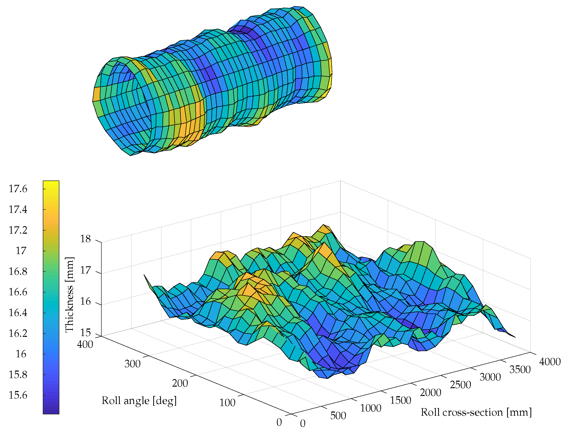[17] combined an extensive rotor-bearing model with multibody approach to perform dynamic analysis of subcritical superharmonic vibrations. As a test case, they considered a paper machine roll with non-idealities such as variation in shell thickness and bearing waviness. Compared to experimental modal analysis, the optimized simulation model was able to accurately predict the half-critical resonance (2X, i.e., the excitation is occurring twice per revolution resulting in resonance peak at half the critical speed), which is significant for such industrial application.

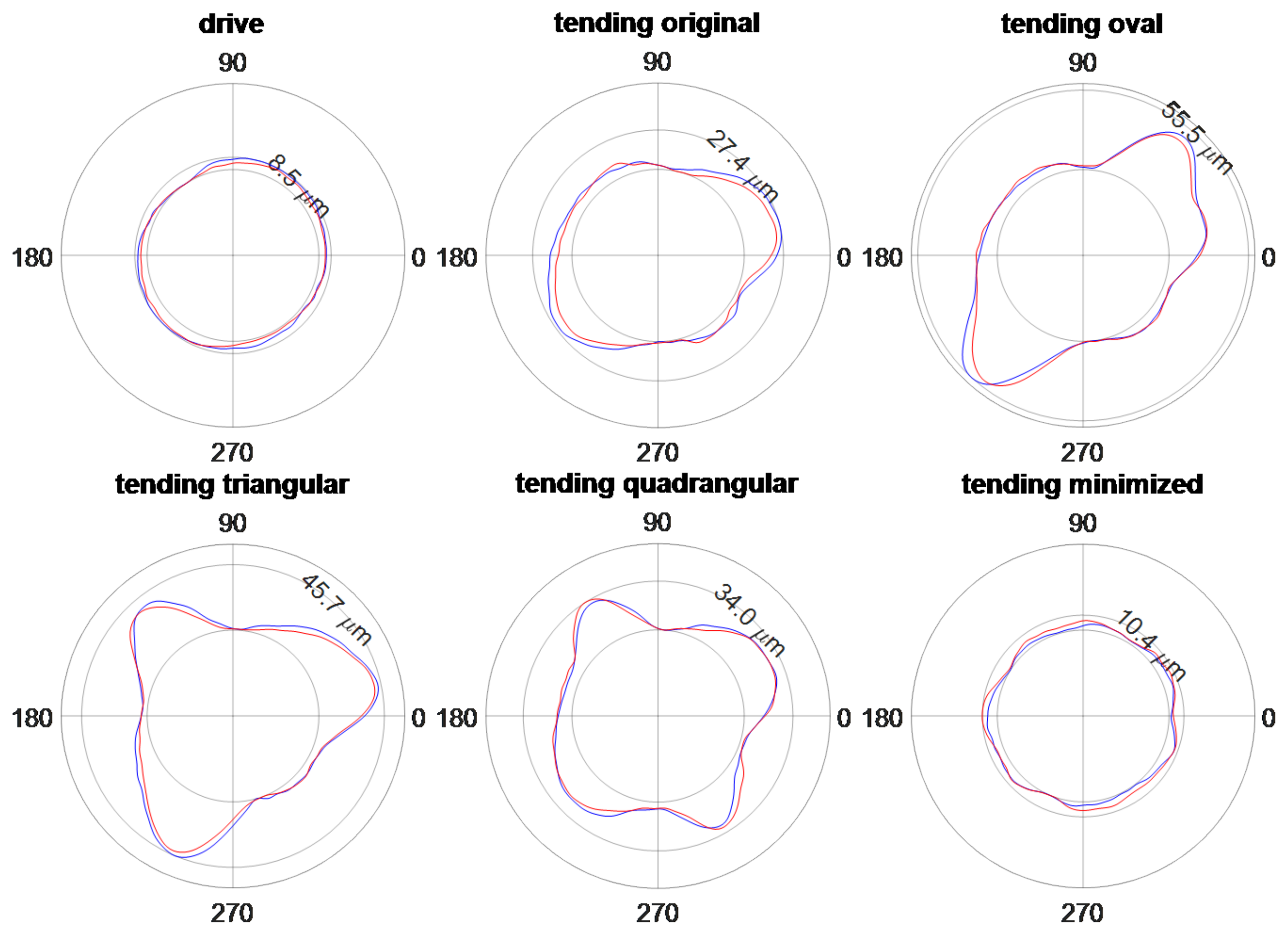
Viitala et al. [18] studied the effect of the bearing inner ring by introducing different roundness profiles and detecting the subcritical vibrations in a paper machine roll. They introduced five different waviness profiles to the inner ring, which was mounted on the rotor shaft. The aim of the study was to minimize the subcritical harmonic resonance responses occurring at half (2X) to one-fourth (4X) times the natural frequency of the first bending mode. This was achieved by minimizing the roundness error of the inner ring. In addition, four other cases with varying roundness profiles were studied for the bearing inner ring. These include the original (as manufactured), oval, triangular, and quadrangular roundness profiles. The different profiles were achieved by insertion of slim metal strips between the bearing installation shaft and the conical adapter sleeve of the bearing.

Heikkinen et al. [19] used asymmetric 3D beam elements to model a paper machine roll to study the subcritical vibrations. The responses from the simulation model were compared with measured responses. In the study, it was concluded that the asymmetry only has a minor effect on the responses, unlike the bearing inner ring roundness profiles, which had a notable effect. The study focused mainly on capturing the half-critical resonance (2X). The 2X frequencies were captured in a reasonable accuracy compared to the measurements. However, as stated by Heikkinen et al. [19], all measured resonance response amplitudes were not repeated accurately by the simulation model. This reveals that other factors are also affecting the results, e.g., damping and as Sopanen and Mikkola [12] revealed, diametral clearance has a great effect on the system response. Harsha [20] studied the radial bearing internal clearance effect in the dynamic response and categorized the responses into three levels: first, very small clearance yields a very linear and predictable system; second, with small clearances, the system response is very sensitive to changes, e.g., rotation speed and clearance; third, chaotic behavior occurs with large clearance. Bearing clearance has an effect on the system dynamics and the 2X response amplitude, as with large clearance (loose bearing) the system excitation is greater than with very small clearance. The clearance is usually very small, within tens of micrometers to hundreds of micrometers and by dissembling the bearing and assembling it back to the rotor, the end result for clearance varies.

The engineering practice in large rotor design is currently widely aware of the vibration problems resulted by half-critical resonance. However, Viitala et al. [18] showed experimentally that remarkable resonance amplitudes can be observed also at one-third (3X) and one-fourth (4X) rotational frequencies. This creates a need to develop efficient and accurate simulation tools to consider these phenomena already in the design phase. The current state-of-the-art commercial FEM software does not include sophisticated nonlinear bearing models that could be used to study, for example, rotor responses due to bearings waviness or defects in a transient domain.

This study presents a novel simulation approach to investigate the frequencies and amplitudes of the first bending mode 2X, 3X, and 4X resonance responses of a large flexible rotor-bearing system subcritical vibration due to varying bearing roundness profile and varying radial bearing clearance. The investigation was limited to harmonic lateral vibration; axial bearing clearance, non-synchronous vibration, torsional, and axial vibrations were neglected. Higher-order harmonic resonance responses were neglected in the present study, since their resonances occur at very low frequencies, which are considered to be outside the operating frequency range in typical applications. The vibration responses obtained by simulation were validated against measurements conducted by Viitala et al. [18].

The results of this study and the resulting simulation method contribute to large rotor design and its dynamical operation optimization. Conceptually, the validated simulation model can be utilized, e.g., to generate teaching datasets for machine learning algorithms to classify certain root failure causes, as in Sobie et al. [21]. Parameters such as bearing clearance, bearing roundness profile, foundation stiffness, external load, material properties, and rotor design can be varied in the proposed simulation model with a systematic approach and doing rapid prototyping in the design phase for the large rotor cases with low effort.

2. Simulation Model and Experimental Setup

This chapter presents the theoretical background and methods of the study. The bearing model and the bearing waviness measurements are presented in Section 2.1. Section 2.2 describes the investigated rotor system, its FEM based model, and the measurement setup, which was used to capture the validating measurement data. Finally, the simulation procedure is introduced in Section 2.3.

2.1. Bearing Modeling and Measurement

2.1.1. Spherical Roller Bearing Model

A spherical roller bearing (SRB) model proposed by Ghalamchi et al. [22] is utilized in this study. In the following, the main aspects of the model as well as modeling of the bearing clearance and inner ring waviness are described. Figure 1 illustrates the radii of curvature of the roller, outer race, and inner race of a spherical roller bearing.

The total elastic deformation of $i^{th}$ rolling element, $j^{th}$ row located at angle ${\beta }_j^i$ can be determined from the relative displacements between the inner and outer races. Based on the geometry, the distance $\left(A_0\right)$ between inner and outer raceway curvature centers $(O_{in}$ and $O_{out})$ can be calculated as [22]

$$A_0=r_{By}^{out}+r_{By}^{in}-d_r-{\displaystyle \frac{c_d}{2}}$$

(1)

where $r_{By}^{out}$ and $r_{By}^{in}$ are inner and outer raceway curvatures, respectively, while $d_r$ is the roller diameter and $c_d$ is the diametral clearance. The displacements for roller i, in row j in the axial direction $\left({\delta }_{zj}^i\right)$ and radial directions $\left({\delta }_{rj}^i\right)$ can be calculated as:

$$\begin{array}{cc}\hfill {\delta }_{zj}^i& =A_{0}sin\left({\varphi }_0\right)+e_z,\hfill \\ \hfill {\delta }_{rj}^i& =A_{0}cos\left({\varphi }_0\right)+e_{x}cos\left({\beta }_j^i\right)+e_{y}sin\left({\beta }_j^i\right),\hfill \end{array}$$

(2)

where $e_x$, $e_y$, and $e_z$ represent the relative displacements between the inner and outer race and ${\varphi }_0$ is the initial contact angle. The contact angle is negative for the 1st row and positive for the 2nd row of the bearing.

The resulting loaded distance, i.e., the distance difference of loaded and non-loaded, for roller i in row j as a function of attitude angle of roller $\left({\beta }_j^i\right)$ can be written as follows:

$$A\left({\beta }_j^i\right)=\sqrt{{\left({\delta }_{zj}^i\right)}^2+{\left({\delta }_{rj}^i\right)}^2}$$

(3)

The compression of a single roll along the common normal as a function of attitude angle due to relative motions of inner and outer rings is

$$d\left({\beta }_j^i\right)=r_{By}^{out}+r_{By}^{in}-A\left({\beta }_j^i\right).$$

(4)

As shown in Equations (1) to (4), the bearing clearance $c_d$ contributes to the contact deformation of individual rollers and thus changes the load distribution between rollers. In case of radially loaded zero-clearance bearing, the load is theoretically distributed to rollers in 180° circumference, while, in case of large clearance, the load can be shared by only few rollers. However, it should be noted that the effect of clearance is not so straightforward in case of non-circular bearing rings with waviness. The bearing inner ring waviness profile is included to the elastic deformation of the roller i in the row j as follows:

$$d_{{\beta }_j^i}^w=\sum _{k=1}^n{c}_{k}cos\left[k\left({\beta }_{ij}-\theta \right)+{\varphi }_k\right],$$

(5)

where $d_{{\beta }_j^i}^w$ is the elastic deformation due the bearing inner ring waviness, ${\beta }_{ij}$ is the angular position of the roller, $\theta$ is the rotation angle of the inner ring, k harmonic waviness order, $c_k$ is the $k^{th}$ order waviness amplitude, and ${\varphi }_k$ is the phase angle of $k^{th}$ order waviness, respectively. The modeling approach assumes that the elastic compression is completely in the rollers while the not-round inner race and perfectly circle outer race are assumed to be rigid.

The total elastic compression for an individual roller can be written as follows:

$${\delta }_{{\beta }_j^i}=d_r-d\left({\beta }_j^i\right)+d_{{\beta }_j^i}^w$$

(6)

In the loaded condition, the contact angle for individual roller elements can be defined as

$${\varphi }_j^i={tan}^{-1}\left({\displaystyle \frac{{\delta }_{zj}^i}{{\delta }_{rj}^i}}\right).$$

(7)

Using Hertzian contact theory, the contact force of each roller having positive contact deformation can be calculated as

$$F_j^i=k_c^{tot}{\left({\delta }_{{\beta }_j^i}\right)}^{1.5},$$

(8)

where $k_c^{tot}$ is the roller contact stiffness coefficient and is calculated as

$$k_c^{tot}={\displaystyle \frac{1}{{\left[{(1/k_c^{in})}^{2/3}+{(1/k_c^{out})}^{2/3}\right]}^{3/2}}}$$

(9)

where $k_c^{in}$ and $k_c^{out}$ are the inner and outer race contact areas, respectively. The total bearing forces in different translational directions can be calculated as a sum of all individual roller forces. Bearing clearance and the waviness of the inner ring consequently affect the total bearing force by changing the internal load distribution of the bearing. In practice, this leads to time-dependent dynamic excitation and time-varying stiffness of the bearing. In this study, the values of clearance ($c_d$) shown in Equation (1) are varied from 10 μm to 120 μm. In addition, the waviness amplitude $c_k$, order of waviness amplitude k and phase of waviness amplitudes ${\varphi }_k$ shown in Equation (5) are varied to the measured values, and these are shown in Section 2.1.2 in

Table 1. Bearing waviness amplitudes used in the simulation model.

	First   Roller  Element  Path		Second  Roller  Element  Path
k	Amplitude (${\mathit{c}}_{\mathit{k}}$) [μm]	Phase (${\mathit{\varphi }}_{\mathit{k}}$) [deg]	Amplitude (${\mathit{c}}_{\mathit{k}}$) [μm]	Phase (${\mathit{\varphi }}_{\mathit{k}}$) [deg]
Service end
Case 1—original
1	0	0	0	0
2	10.035	–40.7	7.1650	–39.3
3	2.6100	80.8	3.0650	75.7
4	4.2350	63.7	4.6950	69.0
Case 2—oval
1	0	0	0	0
2	18.145	–75.7	16.320	–75.9
3	2.2900	86.2	3.0950	71.4
4	9.8300	–0.2	8.4950	–6.7
Case 3—triangular
1	0	0	0	0
2	7.3200	–77.1	6.2200	–66.3
3	16.455	58.7	15.925	57.9
4	4.8250	9.7	4.9350	3.5
Case 4—quadrangular
1	0	0	0	0
2	1.8700	–73.4	1.7800	7.0
3	3.4750	48.0	2.8850	45.7
4	10.280	50.4	10.730	47.8
Case 5—optimized
1	0	0	0	0
2	1.9300	–31.6	1.2100	3.2
3	0.9150	–155.3	1.0700	–115.7
4	0.2900	–196.6	1.2700	–220.4
Drive end
1	0	0	0	0
2	2.9500	–94.5	2.6550	–80.6
3	1.0650	–131.9	0.4300	–177.5
4	0.6700	–169.8	0.9100	–94.5

.

2.1.2. Bearing Waviness Measurement

The rotor was suspended by a double row of spherical roller bearings (SKF 23124 CCK/W33) at both ends (Figure 2). The $d_1$ is the bore diameter, $d_2$ is the approximate inner race diameter at bearing end, $d_r$ roller diameter, D is the outer race diameter, $D_1$ is the outer race approximated inner diameter at bearing end, B is the bearing width, and $B_4$ the lock nut width. In the bearing model, the z is the number of rollers, $n_z$ rows of rollers, $r_{By}^{out}$ outer race contour radius, $r_{By}^{in}$ inner race contour radius, ${\varphi }_0$ is the free contact angle, and $E_{roller}$ and $E_{ring}$ are the Modulus of Elasticity of the roller and rings and ${\nu }_{roller}$ and ${\nu }_{ring}$ the Poisson’s ratios, respectively. The bearing clearance of the experimental rotor system was identified to contain remarkable uncertainty due to several assembly and disassembly procedures of the service sided bearing. The roundness profile of the installed bearing inner ring was modified by inserting thin steel shims between the rotor shaft and the conical bearing adapter sleeve as depicted in Figure 3.

The bearing was disassembled to modify the bearing geometry. The bearing clearance was varied in the simulation model in a controlled manner to investigate its effect on the rotor response.

The bearing inner ring roundness profile was measured while installed on the rotor shaft (Figure 4). This ensured that the acquired roundness profile was the actual roundness profile of the inner ring in the operating conditions.

The roundness profile was measured utilizing the four-point method.[18,23,24]. The four-point method is able to differentiate the roundness profile and the error motion of the workpiece in a reliable way. Traditional roundness measurement machines could not be used due to the large size of the workpiece. Five different roundness profiles of the bearing inner ring were measured at the service end of the rotor: original, oval, triangular, quadrangular, and minimized roundness error. Figure 5 depicts the roundness profiles. The original geometry was measured as such without any intended modification. The drive end was not modified, but the roundness profile was measured nevertheless. Table 1 depicts the values of roundness error including the amplitude and phase of the waviness of different orders that can be combined by means of a Fourier series.

2.2. Studied Rotor System

Figure 6 illustrates the studied rotor system. The rotor is supported by two spherical roller bearings located in both ends. The bearing housings are bolted to 2.5 cm steel plate that is welded to two OD 19.5 cm steel tubes with wall thickness of 2 cm. The other end of the steel tubes are welded to 5 cm thick steel plate that is bolted from the centre to the stiff steel foundation. The rotor is driven though a coupling between the rotor drive-end and electric motor controlled by a frequency converter.

2.2.1. Simulation Model of the Rotor System

The asymmetric rotor is modeled using the Finite Element Method (FEM) including the description of asymmetry. The rotor was modeled employing Timoshenko beam elements. The tubular rotor wall thickness variation was included in the model by defining the area moments of inertia individually for both cross-sectional principal axes as described in [19]. The rotor is supported with a double row of spherical roller bearings (SKF 23124 CCK/W33) that are implemented in the model using the modeling method discussed in Section 2.1.1. In the FE model, the rotor is discretized into 24 beam elements using 25 nodes along the rotor’s length (Figure 7). The discretization facilitates the integrations of other components into the model, using the nodes at each key location of the rotor. Each rotor node has two translational and two rotational degrees of freedom (DOFs). The geometry and physical parameters of the rotor contribute as input to the model. For instance, the bearings are located at nodes 2 and 24. The support is connected at bearing locations with additional nodes. The support structures contribute to the total mass (bearing, bearing housing and the two cylinder bed) an additional mass of 190 kg each at their respective locations. Furthermore, the overhanging part from the tube end modeled as an additional mass point, i.e., not providing additional stiffness to the system, of approximately 6 kg at node 6 and node 20, respectively. Lastly, for the initial balancing of the tube roll, the balancing planes are located at nodes 6 and 20 where a balancing mass of 2.6 kg and 2.8 kg are added at each plane.

The foundation stiffness of the simulation model was defined by utilizing foundation design and the corresponding stiffness values obtained from static FE analysis and then matched with the measured peak response frequencies in the horizontal and vertical directions. The corresponding stiffness values in the horizontal and vertical directions are 18 MN/m and 195 MN/m, respectively. Damping of the support is fine-tuned according to the shape of the measured response curves and the damping ratios are evaluated as 1.3% in the vertical direction and 2.3% in the horizontal direction.

2.2.2. Measurement of the Rotor System

The wall thickness of the tubular rotor is variable due to a commonly used manufacturing method where the rotor is made from a thick sheet plate that is bent into a tubular form, welded and turned from the outer circle. The thickness variation was measured to provide input data for the asymmetric rotor simulation model. Figure 8 depicts the thickness variation [25]. An ultrasound probe was used to measure the rotor shell thickness. Water was used as an ultrasound transmitting medium between probe and the roll. The thickness measurement consisted of 20 measurements along the circumference of the rotor and 36 measurements along the rotor axial direction leading altogether to a measurement grid of 720 points. The result showing thickness variation up to 2 mm, as the nominal thickness was 16.5 mm, is presented in Figure 9.

The experimental rotor system and the measurement results are presented by Viitala et al. [18]. The dynamic response of the rotor was measured utilizing a measurement environment built on a commercial roll grinding machine that was presented previously in Figure 6. The response was measured in horizontal and vertical directions at the middle cross-section of the rotor at a rotational frequency range of 4–18 Hz with 0.2 Hz increments using the four-point method to extract the roundness profile and the rotor center point movement from the measured signals of the four laser sensors. An encoder was used to collect 1024 samples per revolution. A hundred revolutions of data were acquired at each rotational frequency step. The data sets were synchronously averaged to reduce noise and measurement uncertainty [26,27,28]. Finally, the center point movement data was analyzed using FFT to obtain the response spectra of the rotor in horizontal and vertical directions.

2.3. Simulation Procedure

The tubular rotor model dynamic behavior was verified by experimental modal analysis measurements of the loosely supported (free-free) rotor. In the measurement, the rotor was lifted from the pedestal and suspended by flexible ropes in order to obtain the free-free modes. The measured free-free frequencies are 70 Hz for the first bending and 168.5 Hz for the second bending mode. In the model, the first bending frequency is 70 Hz and 179 Hz for the second bending mode. As typical in the beam element-based rotor models, the first bending mode can be tuned well to match the measured frequencies while the second bending mode is usually slightly higher than measured. Next, the bearing model and the description of the foundation stiffness was included in the rotor model. The critical speeds of supported rotor were compared with the measurements to verify the supported model dynamical behavior. The simulation procedure for the created rotor model was conducted in seven steps for each of the 60 studied case as follows:

• Define varying input parameters including bearing clearance and rotational speed
• Define a static equilibrium position of the system
• Analyze transient response of nine-second time span at constant rotational speed
• Convert the transient response into frequency domain using FFT
• Repeat from Step 1 until all rotational speeds are calculated
• Plot response curves as functions of rotational speed i.e., three-dimensional waterfall graph
• Capture subcritical peak responses from waterfall graphs

The simulation was performed in a time domain, i.e., transient response of the rotor was observed. The transient response was studied at constant rotational speed and the simulation started at the equilibrium position of the static rotor. The studied time span was nine seconds and the simulation time step was 0.0005 s. The studied rotational speeds were between 4 and 17 Hz with a 0.05 Hz rotational speed increment resulting in 281 studied rotational speeds. A total of five different cases were studied according to the studied waviness configurations in which the bearing clearance varied from 10 μm to 120 μm with a 10 μm increment. The bearing clearance was identified as one of the key sources for change in the response amplitudes.

The response data in the time domain were converted to frequency domain by Fast Fourier Transform (FFT). In addition, 16,384 FFT points (2000 Hz/16,384 = 0.122 Hz increment) and Hanning windowing was used. The individual response curves in the frequency domain are then plotted as a function of rotation speed generating waterfall graphs for each of the 60 studied cases. The maximum peaks at 1/2, 1/3, and 1/4 rotation speeds are captured from waterfall graphs for further analysis.

3. Results

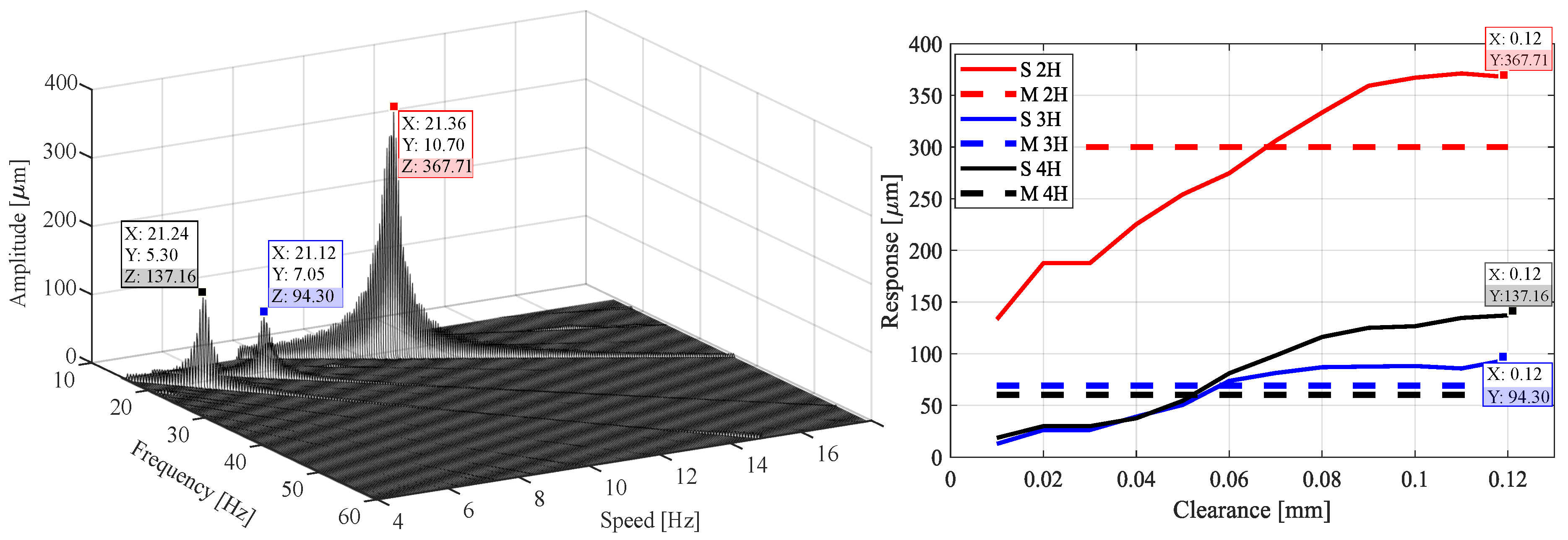
In the simulation model, the responses in the middle cross-section of the rotor were studied, similarly to the measurement by Viitala et al. [18]. The left side of Figure 10 shows a waterfall plot in Case 1 with 120 μm bearing clearance. The resonance peaks of the second, third, and fourth (2H, 3H and 4H) subharmonic response components were studied in both horizontal and vertical directions. On the right side of the figure, the corresponding response peaks are shown in a two-dimensional graph, the x-axis representing the bearing clearance. The response peak values with all bearing geometries (Cases from 1 to 5) with varying bearing clearance (10 μm to 120 μm with 10 μm increment) at the middle of the rotor are shown in the results. The nominal clearance for the bearing is 60 μm. The proposed simulation method enables investigation of the combined effect of the bearing clearance and geometry on the rotor response.

In Figure 11, Figure 12, Figure 13, Figure 14 and Figure 15, the solid lines correspond to the simulated values and the dashed lines to the measured values. In the analysis, the drive end waviness remains fixed and the service end is variable. However, in the simulation, the bearing clearance was changed for the drive end and the service end simultaneously as both clearances were unknown.

3.1. Case 1—Original Bearing Inner Ring Roundness Profile in the Service End

Table 2. Average amplitudes and phases of the two roller element paths (see Figure 5) used in Case 1 for the service end and the drive end. For the phase, the circular average was utilized.

Amplitude   Component	2nd Harmonic	3rd Harmonic	4th Harmonic
Case 1 (service end)	8.60 μm ($-40.1deg$)	2.83 μm ($77.9deg$)	4.46 μm ($66.5deg$)
Case 1 (drive end)	2.78 μm ($-87.67deg$)	0.98 μm ($-154.7deg$)	0.63 μm ($-125.5deg$)

presents the bearing inner ring roundness profile amplitudes and phases used as inputs for the simulation model for the service and drive end. The drive end roundness profile remains the same for cases 1 to 5 while the service end varies according to the studied case. The measured roundness profile was adapted to the simulation model. The highest roundness profile amplitudes were measured for the second harmonic component. Case 1 represents the ’original case’, in which the bearing was installed on the rotor shaft according to the bearing supplier instructions without manual modification.

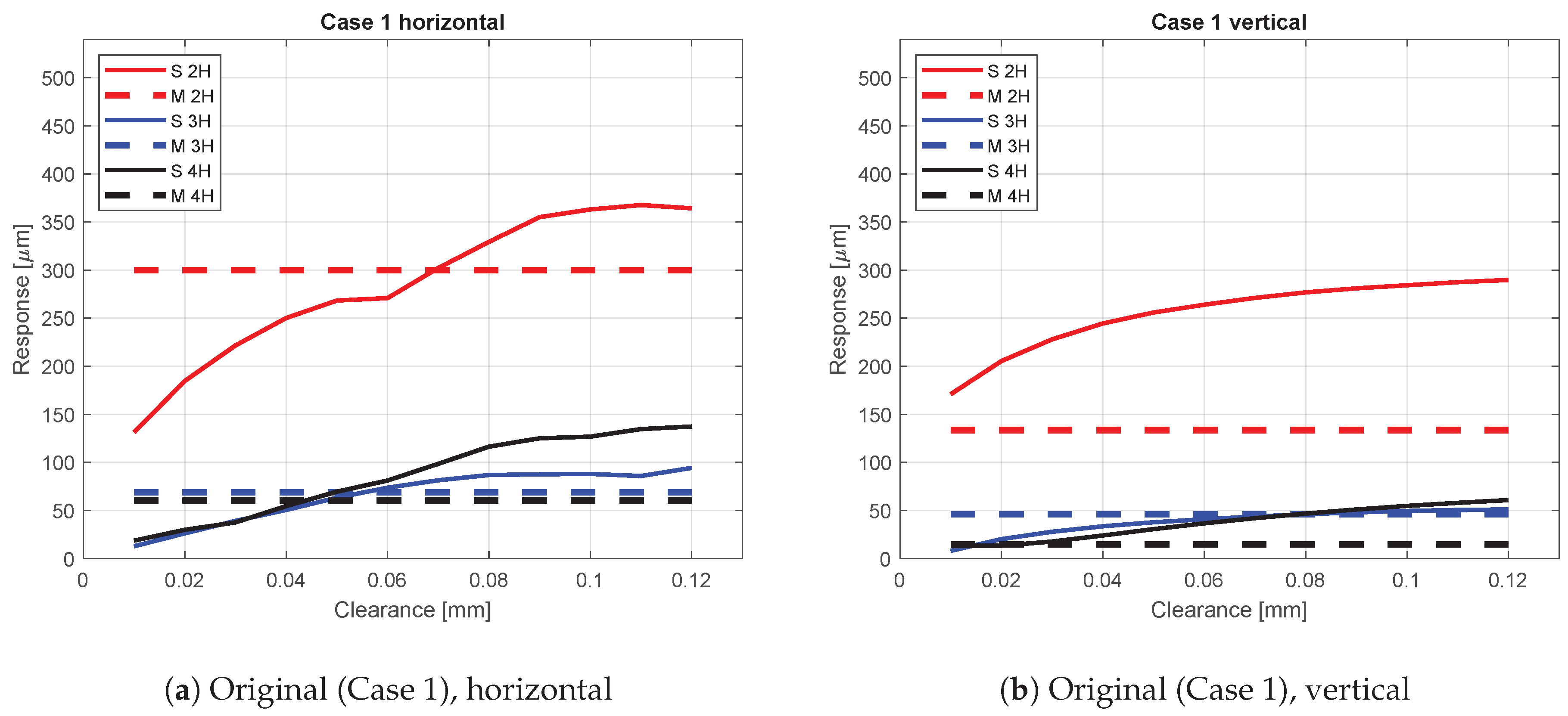
Figure 11 presents the simulation results produced with the original bearing inner ring roundness profile in the service end of the rotor.

Consequently, the results show that larger clearance between the roller elements of the bearing and the bearing outer ring increased the subcritical response amplitudes at the subcritical resonance frequencies. Even though the velocity increment utilized in the simulation model was small (0.05 Hz), some variation can be observed particularly in the horizontal 2nd harmonic component, when the clearance is 0.05–0.06 mm, but, in general, the trend seems clear. Lower change rate can be seen in the vertical direction. However, this relates to the foundation stiffness and is also observed with measured responses. Suggested by the results presented in Figure 11, the clearance value in the range from 0.05 to 0.08 mm provides the best agreement between the simulation and the measurement in horizontal direction. However, some difference can be detected in the vertical 3rd harmonic component, which attains the measured amplitude level in high clearance value. In the vertical direction, the 2nd harmonic component has substantially higher response compared to the measured values.

3.2. Case 2—Oval Bearing Inner Ring Roundness Profile in the Service End

Table 3. Average amplitudes and phases of the two roller element paths (see Figure 5) used in Case 2 for the service end and the drive end. For the phase, the circular average was utilized.

Amplitude Component	2nd Harmonic	3rd Harmonic	4th Harmonic
Case 2 (service end)	17.23 μm ($-75.7deg$)	2.67 μm ($77.7deg$)	9.15 μm ($-3.2deg$)
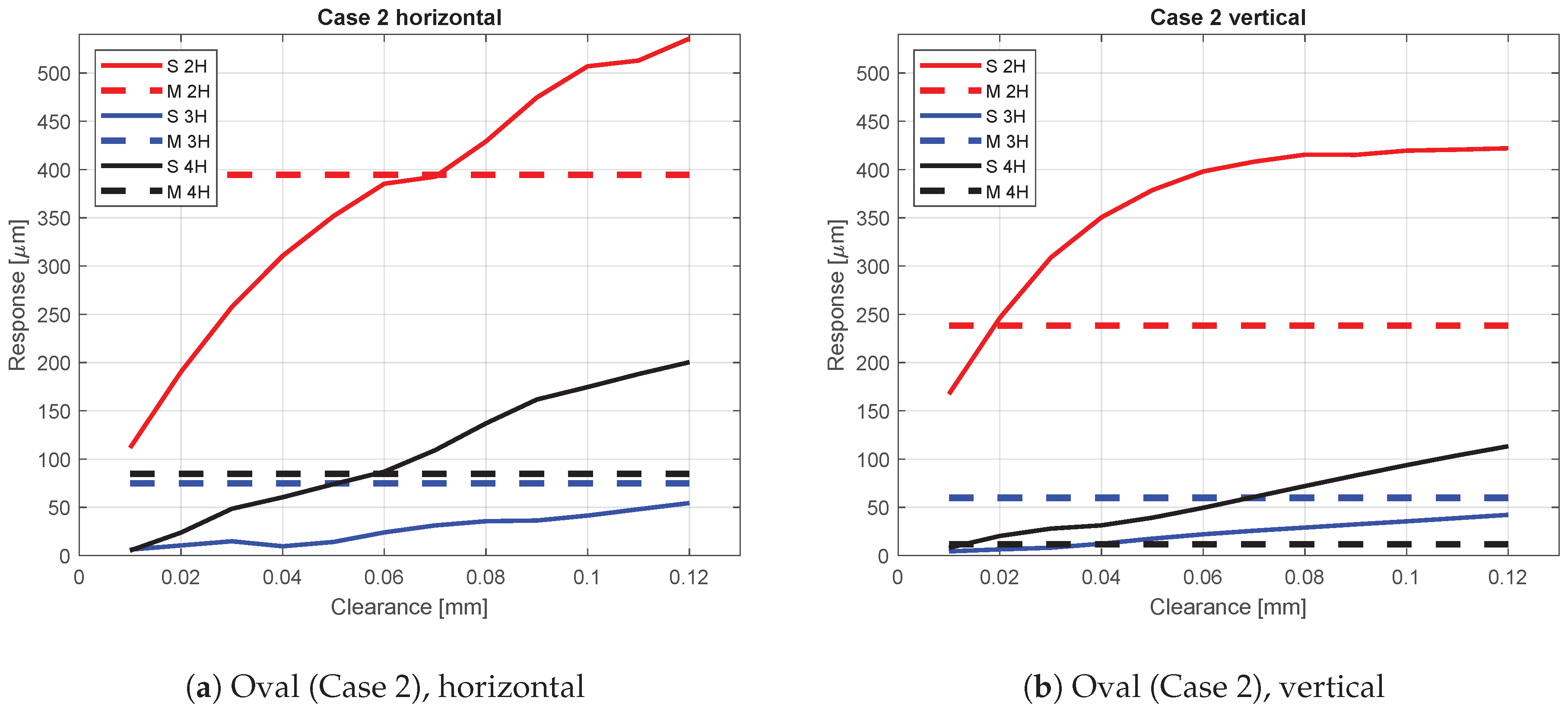
Case 2 (drive end)	2.78 μm ($-87.67deg$)	0.98 μm ($-154.7deg$)	0.63 μm ($-125.5deg$)

presents the bearing inner ring roundness profile amplitudes and phases used as inputs for the simulation model. In the second case, the amplitude of the second harmonic roundness component was intentionally increased using thin steel shims between the shaft and the conical adapter sleeve.

The results are presented as a function of the bearing clearance. Again, the response amplitudes at subcritical resonances (2H, 3H, and 4H) are shown. The simulation model clearly reacted to the increased 2nd harmonic roundness component of the bearing inner ring with elevated second harmonic response amplitudes. The 2nd and the 4th harmonic component in the horizontal direction behaved similarly compared to Case 1. However, the 3rd harmonic component increased only moderately with the increasing clearance and remained clearly lower than in the original case also with the largest clearances. Accordingly, the highest increases were in the 2nd and 4th harmonic components of the bearing inner ring roundness profile, whereas the 3rd harmonic roundness component remained almost the same compared to the original bearing geometry.

The main effect on the vertical direction response can be seen in the increased 2nd harmonic component, especially with larger clearance values. The 3rd and 4th harmonic component changed only slightly; similar to the horizontal response, the 3rd harmonic remained even lower than in the original case, and the 4th harmonic increased notably more with the inclining clearance. These remarks apply both to the measured and simulated responses.

The results presented in Figure 12 show that the simulated clearance value has divergence when trying to find agreement with the measurement result presented with the dashed line. Horizontal direction 2nd and 4th harmonic components as well as vertical direction 4th harmonic component suggest a clearance of 0.06–0.07 mm. However, in the vertical direction, the 2nd harmonic attains the measured response at 0.01–0.02 mm clearance and 4th harmonic in vertical direction at 0.01 mm clearance. The 3rd harmonic in the horizontal and vertical directions did not attain the measured amplitude at all.

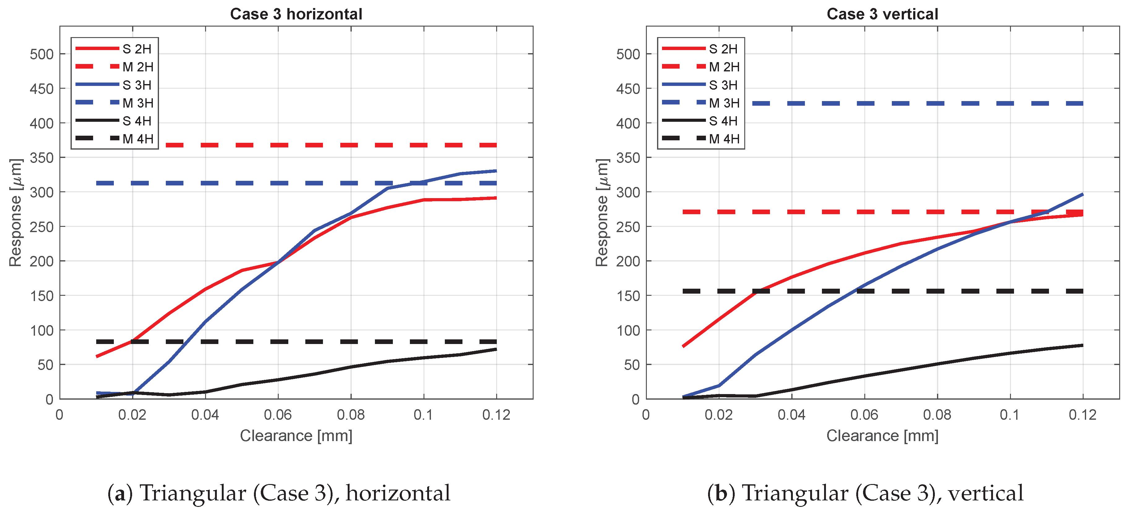
3.3. Case 3—Triangular Bearing Inner Ring Roundness Profile in the Service End

Table 4. Average amplitudes and phases of the two roller element paths (see Figure 5) used in Case 3 for the service end and the drive end. For the phase, the circular average was utilized.

Amplitude Component	2nd Harmonic	3rd Harmonic	4th Harmonic
Case 3 (service end)	6.74 μm ($-72.2deg$)	16.19 μm ($58.3deg$)	4.87 μm ($6.6deg$)
Case 3 (drive end)	2.78 μm ($-87.67deg$)	0.98 μm ($-154.7deg$)	0.63 μm ($-125.5deg$)

presents the bearing inner ring roundness profile amplitudes and phases used as inputs for the simulation model. The roundness profile of the bearing inner ring in the service end was intentionally modified to a triangular geometry. As a consequence, the 3rd harmonic horizontal resonance had the largest amplitude.

Figure 13 presents the simulation results produced with the triangular bearing inner ring roundness profile in the service end of the rotor.

In the horizontal direction, the simulation model reacts clearly to the increased 3rd harmonic roundness component. Hence, the 3rd harmonic resonance peak response attains the measured value with a clearance circa 0.09 mm. The 2nd and 4th harmonic components incline as well with the increasing clearance, however, does not attain the measured response values.In contrast, the vertical direction result shows a disagreement between the simulation model and the measurement. The 2nd and the 3rd harmonic components increased significantly more with the increasing clearance than in the previous cases, but all the components were notably far from the measured values.

With clearance values from 0.01 mm to 0.03 mm, a decrease or a very low increase in the 3rd harmonic response of both directions can be observed. This may be explained with the 3rd harmonic roundness component of the bearing inner ring, which was circa 16 μm (0.016 mm), creating a ’three-point support’, and thus preventing the bearing excitation three times per revolution with smaller bearing clearances.

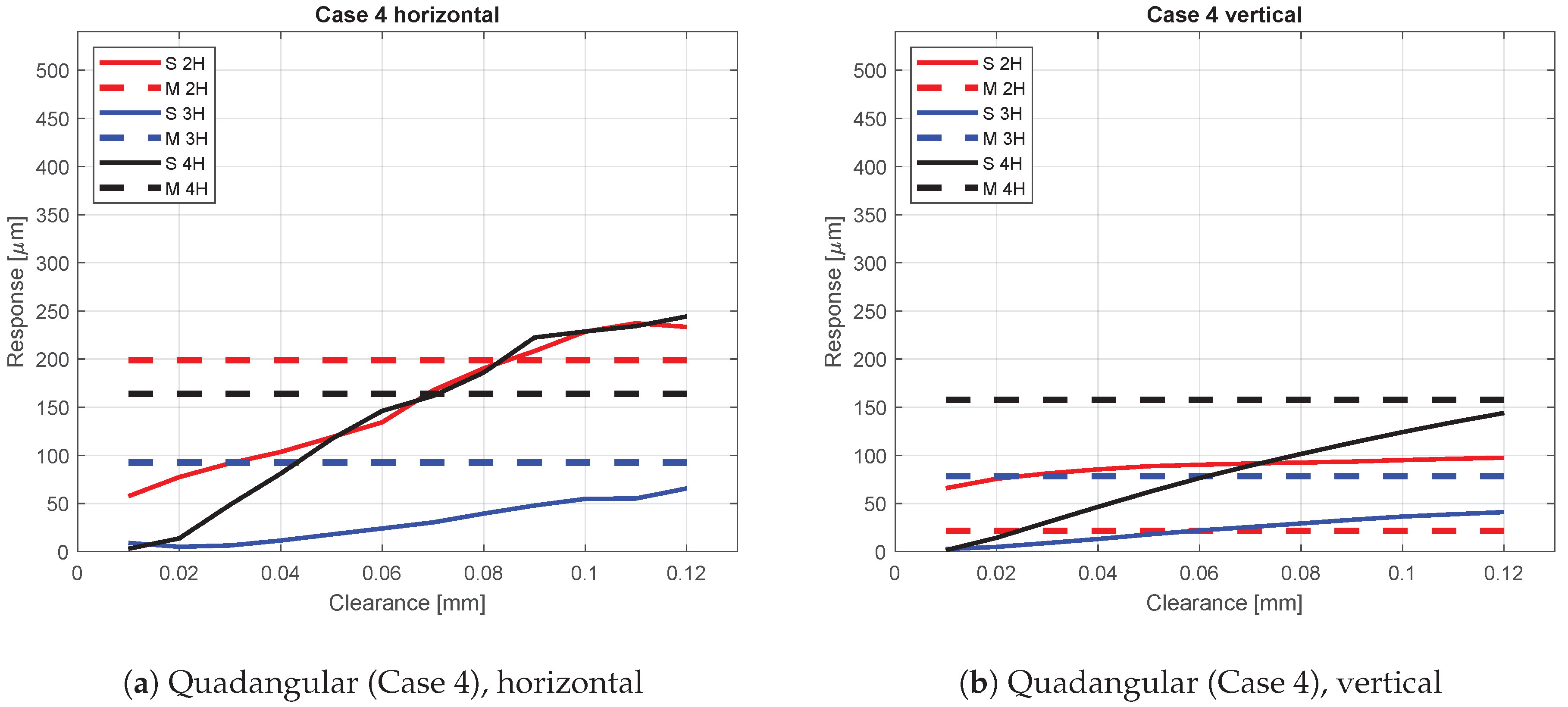
3.4. Case 4—Quadrangular Bearing Inner Ring Roundness Profile in the Service End

Table 5. Average amplitudes and phases of the two roller element paths (see Figure 5) used in Case 4 for the service end and the drive end. For the phase, the circular average was utilized.

Amplitude Component	2nd Harmonic	3rd Harmonic	4th Harmonic
Case 4 (service end)	1.39 μm ($-34.4deg$)	3.18 μm ($46.9deg$)	10.50 μm ($49.5deg$)
Case 4 (drive end)	2.78 μm ($-87.67deg$)	0.98 μm ($-154.7deg$)	0.63 μm ($-125.5deg$)

presents the bearing inner ring roundness profile amplitudes and phases used as inputs for the simulation model. In the fourth case, the amplitude of the fourth harmonic roundness component was intentionally increased. As a consequence, the 4H component had the largest amplitude.

Figure 14 presents the simulation results produced with the quadrangular bearing inner ring roundness profile in the service end of the rotor.

The simulation model clearly reacts to the quadrangularity with elevated 4th harmonic response of the rotor in both horizontal and vertical directions. The 3rd harmonic roundness component has a very low value (in the order of 3 μm), which may partly explain the attenuated 3rd harmonic responses.

The vertical direction 4th harmonic response is limited compared to measurement, but presents, however, a clear increase with increasing bearing clearance. The measured 2nd harmonic response in the vertical direction was very low and the simulated response surpasses it clearly.

The horizontal direction of the 2nd and 3rd harmonic components suggests a clearance in the range of 0.07–0.08 mm. However, other components present significantly divergent results.

Similar to Case 3, a very low increase can be observed in the horizontal 4th harmonic component with clearance values from 0.01 mm to 0.02 mm. The explanation may be the same, now consequently ’four-point support’ preventing the bearing-based excitation four times per revolution with smaller bearing clearances.

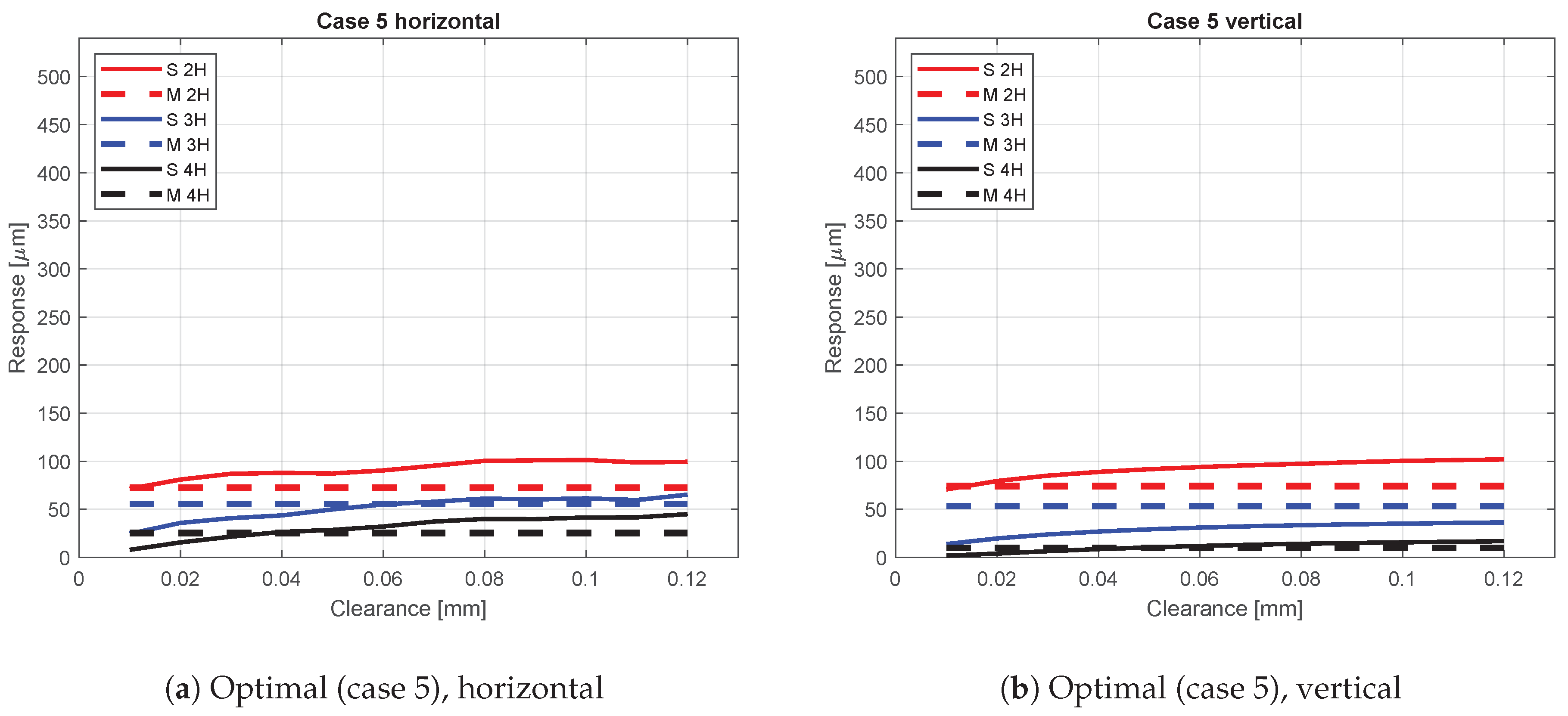
3.5. Case 5—Minimized Roundness Error of the Bearing Inner Ring in the Service End

Table 6. Average amplitudes and phases of the two roller element paths (see Figure 5) used in Case 5 for the service end and the drive end. For the phase, the circular average was utilized.

Amplitude Component	2nd Harmonic	3rd Harmonic	4th Harmonic
Case 5 (service end)	1.50 μm ($-18.3deg$)	0.93 μm ($-133.8deg$)	0.77 μm ($143.9deg$)
Case 5 (drive end)	2.78 μm ($-87.67deg$)	0.98 μm ($-154.7deg$)	0.63 μm ($-125.5deg$)

presents the bearing inner ring roundness profile amplitudes and phases used as inputs for the simulation model. In the fifth case, the roundness error, and thus also the amplitude of all the roundness components, was minimized with thin steel shims. As a consequence, all the roundness components had relatively small amplitudes.

Figure 15 presents the simulation results produced with the optimized bearing inner ring roundness profile in the service end of the rotor.

The measured results showed evidently the lowest total response of the rotor. The simulation model also produced the lowest responses. In the horizontal direction, the 2nd harmonic component measured and simulated responses coincide already with the smallest clearance. The 3rd and 4th harmonic component responses suggests clearance of 0.04–0.06 mm. In the vertical direction, the simulated 2nd harmonic response exceeds the measured response at 0.02 mm clearance and 3rd harmonic response does not attain the measured response even at the highest clearance. The 4th harmonic response in the vertical direction suggest clearance of 0.05–0.06 mm. The results of Case 5 show the lowest growth of the response amplitudes against the bearing clearance.

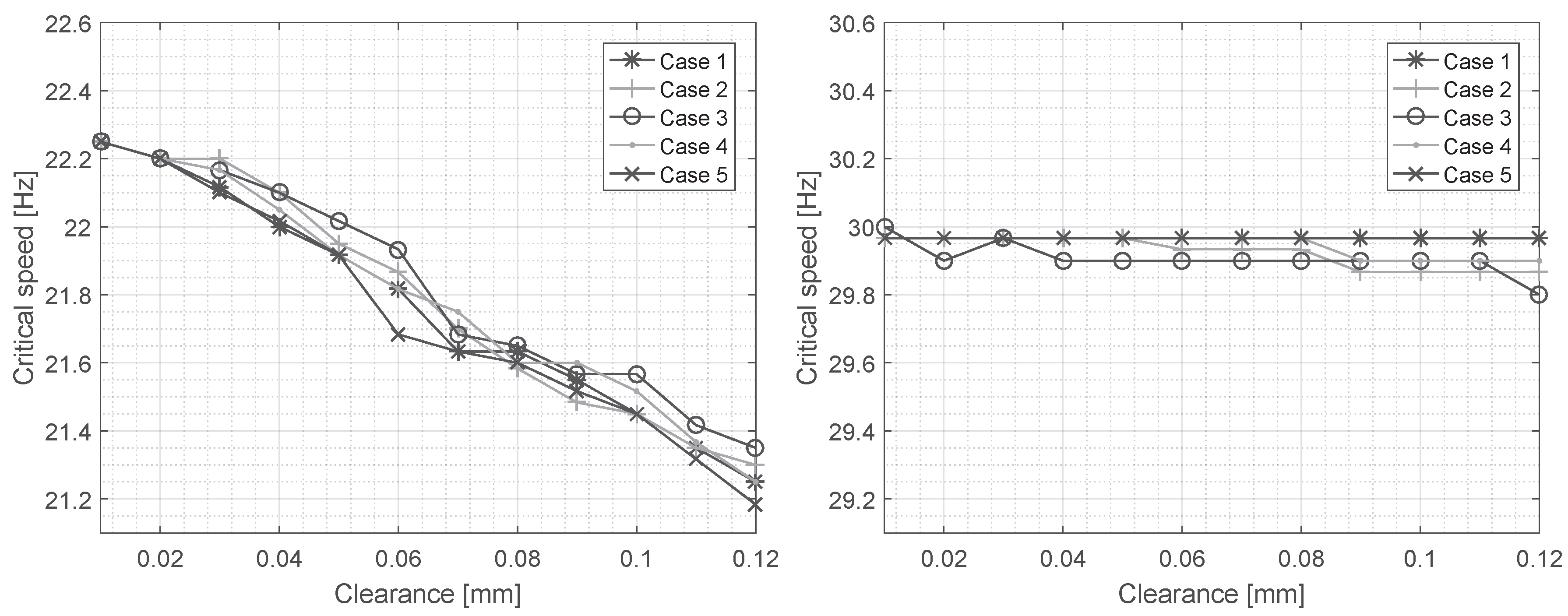
3.6. Bearing Clearance Effect on the Critical Speeds

Figure 16 depicts the average critical speeds in cases from 1 to 5 with respect to the bearing clearance. The average critical speeds were obtained by calculating the average of the critical speeds of the subcritical harmonic resonance frequencies. For example, multiplying 2H resonance frequency by 2, multiplying 3H resonance frequency by three and multiplying 4H resonance frequency by four and finally taking the average yielded the average critical speed. The measured average values for Cases 1 to 5 in horizontal direction 21.7 Hz, 21.7 Hz, 21.2 Hz, 21.4 Hz, and 20.8 Hz showing trend of decreasing the critical speed and having variation range of 0.9 Hz and in a vertical direction 30.1 Hz, 29.8 Hz, 29.9 Hz, 29.9 Hz, and 29.9 Hz showing small decrease in the critical speed by the cases and having a total range in 0.3 Hz.

The critical speeds presented in Figure 16 show a clearly decreasing trend with the increasing bearing clearance, especially in the horizontal direction. In the vertical direction, the critical speed remains merely the same in cases 1 to 5. Comparison of the horizontal direction critical speed between the measurement (21.6 Hz) and the simulation (Figure 16 left) suggests that the bearing clearance was circa 0.07–0.09mm.

4. Discussion

The present study introduces a rotor-bearing system simulation model, which takes the bearing clearance into account and is able to emulate the bearing inner ring waviness. The results suggest that the simulation model output reacts clearly to the varying bearing inner ring roundness profile and the bearing clearance. The frequencies of the subcritical resonance peaks were captured accurately compared to a measurement case used for validating, suggesting that the simulation model is able to predict the critical speeds of the rotor system in horizontal and vertical directions. Separated critical speed suggests a clear difference in the foundation stiffnesses of the horizontal and vertical directions. The response amplitudes of the subcritical resonance peaks were investigated in five different cases with varying bearing clearance. The accuracy of the amplitude capture was found reasonable, despite the fact that variations in different cases were detected in comparison against the validating measurement case.

4.1. Results Compared to the Validating Measured Rotor System

Both the simulation model and the measurements suggest that the rotor system has a different stiffness in horizontal and vertical directions. This can be observed from the natural frequency estimates calculated from the subcritical resonance peak frequencies (see Figure 16) and generally lower amplitudes in the vertical direction. Consequently, the structure of the test bench provides a stiffer foundation in the vertical direction, and, since the simulation model mimicked the measurement test bench, the phenomenon was successfully seen in the simulation results.

In Case 1, the simulated and measured responses were very well aligned in horizontal and vertical directions. In addition, the measured and simulated results coincide close to the 50–70 μm bearing clearance (except vertical 2nd and 3rd harmonic responses). This suggests that 60 μm bearing clearance at both the drive end and service end bearings results in an almost similar behavior that was measured.

In Case 2, the increase of the 2nd harmonic amplitude was clearly captured in the simulation results in both horizontal and vertical directions. Compared to the measurements, the simulated 4th harmonic resonance response had higher responses than the measured values. In the vertical direction, the simulated 3rd harmonic responses were lower than the measured values.

In the horizontal direction of Case 3, the responses obtained with the simulation model were well aligned with the measured values. However, in the vertical direction, the measured values showed substantially higher responses compared to the other four cases, being even higher than the horizontal direction responses. Compared to the simulation, the responses were off by a factor of three. In general, the Case 3 vertical responses were significantly higher compared to the vertical direction amplitudes in the other four cases. The average waviness component amplitudes of the bearing roundness profile (2nd 6.74 μm, 3rd 16.19 μm and 4th 4.87 μm) were at a similar range compared to the other cases. The measurement result in this particular case might be erroneous or 3rd harmonic waviness consequently results in a dynamic phenomenon, which was not captured using the simulation model.

In Cases 3 and 4 (Figure 13 and Figure 14), very limited responses for 3rd and 4th harmonic components were obtained with small bearing clearances. The authors suggest that, because the waviness amplitudes are larger than the bearing clearance, there is no room for 3X and 4X excitations and thus the response is attenuated.

In Case 4, the 2nd and 4th harmonic components showed the highest responses, even though the 4th harmonic bearing roundness profile component had clearly the highest input amplitude. In addition, in most other cases, the 2nd harmonic vibration resonance remained dominant. There are many other sources for 2X excitation as well, such as bending stiffness variation of the tubular rotor, which partially provides an explanation for this phenomenon.

In Case 5, the simulated 2nd harmonic response in the horizontal and vertical directions reached the highest responses already at low clearance values. In the horizontal direction, 3rd and both horizontal and vertical direction 4th harmonics reach equal responses compared to the measured case approximately at a 60 μm clearance range.

4.2. Uncertainties in Capturing the Peak Responses

The accuracy of capturing the response peaks in the simulation and in the measured validation case relates consequently to the sampling rate and the resolution of rotational frequency steps of the rotor, as the resonance peak occurs at a certain frequency. Coarse resolution results in missing the highest values of the response peaks. In the measurements, a rotational speed increment of 0.2 Hz was used. This was identified to be one of the sources causing uncertainty in the results, consequently leading to lower resonance responses. In contradiction, a 0.05 Hz rotational speed increment was used in the simulation, which resulted in a relatively low uncertainty in capturing the highest response peaks. Increasing the resolution in future studies is considered to reduce the uncertainty and to increase the quality of the resulting data sets.

Foundation stiffness has a significant impact on critical speeds, as suggested by the results of the present study as well. The horizontal direction foundation stiffness was approximately one-tenth of the vertical direction stiffness, resulting in critical speeds of 21.6 Hz and 30.0 Hz in horizontal and vertical directions, respectively.

4.3. Limitations and Further Research

In the simulation model, the bearing clearance was varied simultaneously for the drive end and the service end. However, in the actual system, the clearances were not identified or controlled, which could be considered in future studies. The bearing clearance was also changing due to different case studies since the bearing was disassembled and assembled multiple times during the measurement procedure. In future considerations, an accurate method to measure the bearing clearance should be investigated to reduce the uncertainty of the input parameters to the simulation model. In addition, the bearing model may have to be improved to include the flexibility of the outer race to provide an accurate bearing excitation mechanism and thus capture dynamic responses more accurately.

In the vertical direction, the responses obtained via simulation are generally lower than what was obtained with measurements in all cases. This suggests that the bearing outer race roundness error could affect the responses. In the simulation model, the assumption of a rigid bearing outer race is used, and thus the flexibility of the outer race is neglected. The flexibility and roundness profile of the outer race are topics of further research and could explain the lower responses in the vertical direction compared to the measured ones.

4.4. Practical Considerations

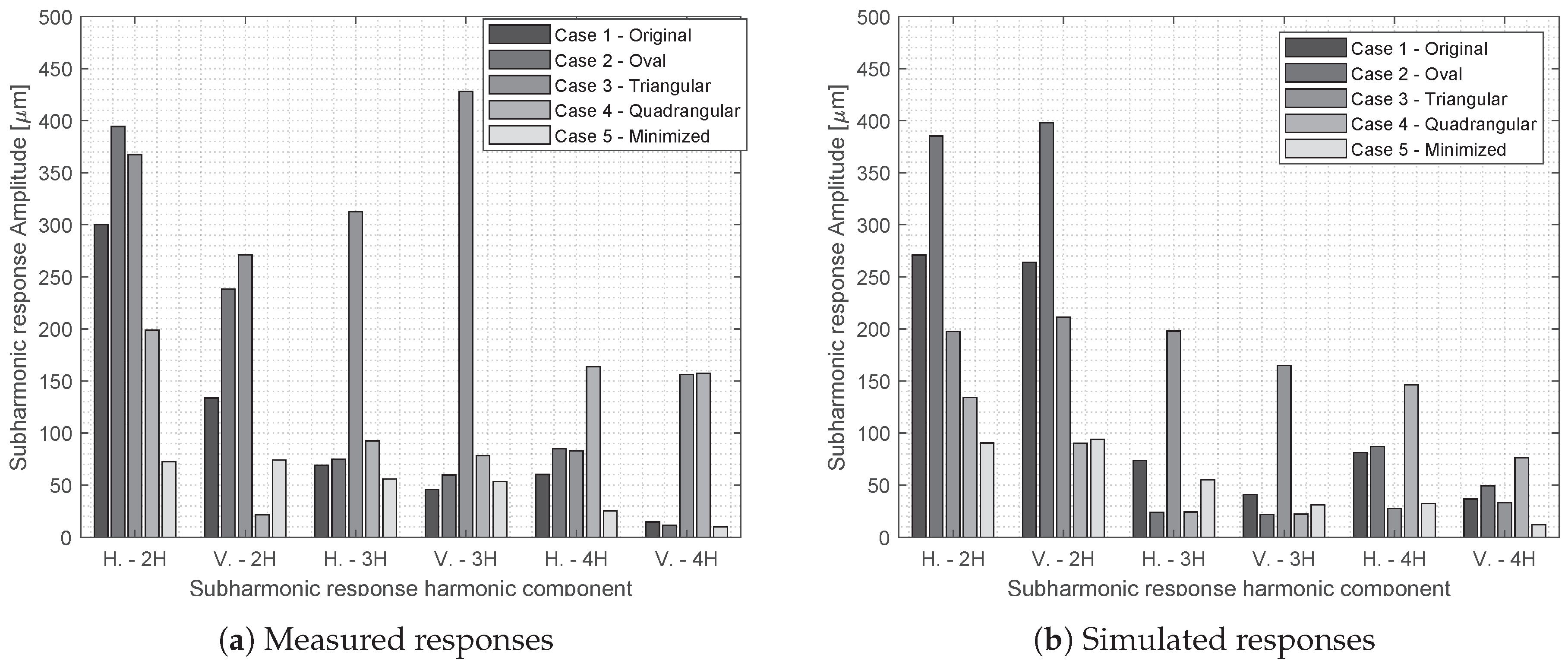
The rotor system simulation model including a rotor modeled using FEM combined with a spherical roller element bearing model resulted in similar behavior as was observed in a validating measurement case. Figure 17 depicts the harmonic response components in horizontal and vertical directions and their amplitudes on the cases 1 to 5. On the left are the measured responses and left the simulated responses at nominal bearing clearance (60 $\mathsf{\mu }$m). It compares the 3rd and 4th harmonic response of the rotor to the well-known 2nd harmonic component for all the cases, and as hypothesized in the research, the figure shows that those components have significant contribution to the rotor response.

The bearing inner ring waviness was observed to have a notable effect on the rotor subcritical behavior, as was discussed by Viitala et al. [18], and now confirmed also by the present simulation study. As a similar behavior could be replicated with the simulation model, it suggests that the bearing excitations and the 3rd and 4th harmonic vibration resonances, in addition to the industrially well-known 2nd harmonic (half-critical), could be considered already in the design phase of large flexible rotors. In addition, it was pointed out and confirmed by Sopanen and Mikkola [12] and Harsha [20] that the rolling element bearing clearance has a great effect on the observed responses. For example, in Case 2 in the horizontal direction, the second subharmonic response with a 10 μm bearing clearance resulted in a circa 120 μm response and with 120 μm bearing clearance over a 540 μm response indicating a magnitude difference of factor 4.5. In practical engineering, this result promotes the importance of assembling the bearings using the correct clearance, or to select a bearing with small clearance.

Another practical way of using the simulation model is generating teaching data for machine learning. The simulation model could be used for computing tens of thousands of different scenarios, e.g., by varying the bearing clearance, material properties, rotor design and foundation stiffness components. Providing a similar data set through measurements is hardly possible and would require an unavailable amount of time and resources. The resulting data-based model could be used as a proxy to the simulation model to predict rotor behavior in various states with low computational effort and time. In addition, various kinds of virtual sensors could be created using the simulation model to generate the virtual measurement data.

5. Conclusions

The present study introduces a novel rotor-bearing system simulation approach, which takes the bearing clearance and the bearing waviness carefully into account and investigates their effect on the subcritical rotor response. The simulation model was validated with measured responses of a large-scale flexible rotor system, where different roundness profiles of the supporting bearing inner ring were introduced. The measurement results confirm the simulation results, which show that the bearing inner ring roundness errors have a great impact on the dynamic behavior of the rotor. The bearing clearance was identified to have a great effect on the subcritical resonance response peaks, and thus it should be carefully considered when assembling bearings. The rotor response in the middle inclined three-fold by increasing the bearing clearance within the defined realistic clearance range. This kind of behavior consequently increases the wear of the rotor-bearing system components and the need of maintenance, and decreases the quality of end product in industries, such as paper, steel, and non-ferrous metal manufacturing, in which the end product is manipulated, formed, and transferred with the surface of such rotors. In addition, the 3rd and 4th harmonic resonance components were found to have notable responses, which suggests considering those already in the design phase in addition to the industrially well-known half critical (2nd harmonic) response.

References

1. Nelson, H.D. A finite rotating shaft element using Timoshenko beam theory. J. Mech. Des. 1980, 102, 793–803. [Google Scholar] [CrossRef]
2. Jei, Y.G.; Lee, C.W. Finite element model of asymmetrical rotor-bearing systems. KSME J. 1988, 2, 116–124. [Google Scholar] [CrossRef]
3. Kang, Y.; Shih, Y.P.; Lee, A.C. Investigation on the steady-state responses of asymmetric rotors. J. Vib. Acoust. 1992, 114, 194–208. [Google Scholar] [CrossRef]
4. Ganesan, R. Effects of bearing and shaft asymmetries on the instability of rotors operating at near-critical speeds. Mech. Mach. Theory 2000, 35, 737–752. [Google Scholar] [CrossRef]
5. Wardle, F. Vibration forces produced by waviness of the rolling surfaces of thrust loaded ball bearings Part 1: Theory. Proc. Inst. Mech. Eng. Part J. Mech. Eng. Sci. 1988, 202, 305–312. [Google Scholar] [CrossRef]
6. Wardle, F. Vibration Forces Produced by Waviness of the Rolling Surfaces of Thrust Loaded Ball Bearings Part 2: Experimental Validation. Proc. Inst. Mech. Eng. Part J. Mech. Eng. Sci. 1988, 202, 313–319. [Google Scholar] [CrossRef]
7. Meyer, L.; Ahlgren, F.; Weichbrodt, B. An Analytic Model for Ball Bearing Vibrations to Predict Vibration Response to Distributed Defects. J. Mech. Des. 1980, 102, 205–210. [Google Scholar] [CrossRef]
8. Aktürk, N. The Effect of Waviness on Vibrations Associated Witli Ball Bearings. J. Tribol. 1999, 121, 667–677. [Google Scholar] [CrossRef]
9. Arslan, H.; Aktürk, N. An investigation of rolling element vibrations caused by local defects. J. Tribol. 2008, 130, 041101. [Google Scholar] [CrossRef]
10. Harsha, S.; Kankar, P. Stability analysis of a rotor bearing system due to surface waviness and number of balls. Int. J. Mech. Sci. 2004, 46, 1057–1081. [Google Scholar] [CrossRef]
11. Zhang, X.; Han, Q.; Peng, Z.; Chu, F. A comprehensive dynamic model to investigate the stability problems of the rotor–bearing system due to multiple excitations. Mech. Syst. Signal Process. 2016, 70, 1171–1192. [Google Scholar] [CrossRef]
12. Sopanen, J.; Mikkola, A. Dynamic model of a deep-groove ball bearing including localized and distributed defects. Part 1: Theory. Proc. Inst. Mech. Eng. Part J.-Multi-Body Dyn. 2003, 217, 201–211. [Google Scholar] [CrossRef]
13. Sopanen, J.; Mikkola, A. Dynamic model of a deep-groove ball bearing including localized and distributed defects. Part 2: Implementation and results. Proc. Inst. Mech. Eng. Part J.-Multi-Body Dyn. 2003, 217, 213–223. [Google Scholar] [CrossRef]
14. Liu, W.; Zhang, Y.; Feng, Z.J.; Zhao, J.S.; Wang, D. A study on waviness induced vibration of ball bearings based on signal coherence theory. J. Sound Vib. 2014, 333, 6107–6120. [Google Scholar] [CrossRef]
15. Halminen, O.; Aceituno, J.F.; Escalona, J.L.; Sopanen, J.; Mikkola, A. A touchdown bearing with surface waviness: A dynamic model using a multibody approach. Proc. Inst. Mech. Eng. Part J. -Multi-Body Dyn. 2017, 231, 658–669. [Google Scholar] [CrossRef]
16. Halminen, O.; Aceituno, J.F.; Escalona, J.L.; Sopanen, J.; Mikkola, A. A touchdown bearing with surface waviness: Friction loss analysis. Mech. Mach. Theory 2017, 110, 73–84. [Google Scholar] [CrossRef]
17. Sopanen, J.; Heikkinen, J.; Mikkola, A. Experimental verification of a dynamic model of a tube roll in terms of subcritical superharmonic vibrations. Mech. Mach. Theory 2013, 64, 53–66. [Google Scholar] [CrossRef]
18. Viitala, R.; Widmaier, T.; Kuosmanen, P. Subcritical vibrations of a large flexible rotor efficiently reduced by modifying the bearing inner ring roundness profile. Mech. Syst. Signal Process. 2018, 110, 42–58. [Google Scholar] [CrossRef]
19. Heikkinen, J.E.; Ghalamchi, B.; Viitala, R.; Sopanen, J.; Juhanko, J.; Mikkola, A.; Kuosmanen, P. Vibration analysis of paper machine’s asymmetric tube roll supported by spherical roller bearings. Mech. Syst. Signal Process. 2018, 104, 688–704. [Google Scholar] [CrossRef]
20. Harsha, S. Nonlinear dynamic response of a balanced rotor supported by rolling element bearings due to radial internal clearance effect. Mech. Mach. Theory 2006, 41, 688–706. [Google Scholar] [CrossRef]
21. Sobie, C.; Freitas, C.; Nicolai, M. Simulation-driven machine learning: Bearing fault classification. Mech. Syst. Signal Process. 2018, 99, 403–419. [Google Scholar] [CrossRef]
22. Ghalamchi, B.; Sopanen, J.; Mikkola, A. Simple and versatile dynamic model of spherical roller bearing. Int. J. Rotating Mach. 2013, 2013. [Google Scholar] [CrossRef]
23. Widmaier, T.; Hemming, B.; Juhanko, J.; Kuosmanen, P.; Esala, V.P.; Lassila, A.; Laukkanen, P.; Haikio, J. Application of Monte Carlo simulation for estimation of uncertainty of four-point roundness measurements of rolls. Precis. Eng. 2017, 48, 181–190. [Google Scholar] [CrossRef]
24. Viitala, R.; Widmaier, T.; Hemming, B.; Tammi, K.; Kuosmanen, P. Uncertainty analysis of phase and amplitude of harmonic components of bearing inner ring four-point roundness measurement. Precis. Eng. 2018, 54, 118–130. [Google Scholar] [CrossRef]
25. Juhanko, J.; Porkka, E.; Widmaier, T.; Kuosmanen, P. Dynamic geometry of a rotating cylinder with shell thickness variation. Est. J. Eng. 2010, 16, 285. [Google Scholar] [CrossRef] [Green Version]
26. McFadden, P. A revised model for the extraction of periodic waveforms by time domain averaging. Mech. Syst. Signal Process. 1987, 1, 83–95. [Google Scholar] [CrossRef]
27. Braun, S. The synchronous (time domain) average revisited. Mech. Syst. Signal Process. 2011, 25, 1087–1102. [Google Scholar] [CrossRef]
28. McFadden, P.; Toozhy, M. Application of synchronous averaging to vibration monitoring of rolling element bearings. Mech. Syst. Signal Process. 2000, 14, 891–906. [Google Scholar] [CrossRef]
Figure 1. Parameters in a spherical roller bearing and radii of curvature of the roller, outer race, and inner race, and axial and transverse cross-sections of the studied bearing.
Machines 08 00028 g001
Figure 2. Spherical roller bearing SKF 23124 CCK/W33 with conical adapter sleeve H 3124. Both rows contain 21 roller elements.
Machines 08 00028 g002
Figure 3. The bearing inner ring roundness profile was modified by inserting steel shims between the conical adapter sleeve and the rotor shaft [18].
Machines 08 00028 g003
Figure 4. The bearing inner ring roundness profile was measured while installed on the rotor shaft [24].
Machines 08 00028 g004
Figure 5. The roundness profiles of the installed bearing inner ring. The two profiles indicated in red and blue represent the roundness profiles in the middle of both roller paths of the bearing inner ring. The roundness error value in the figure represents the larger roundness error of the red and blue curve. The service end bearing inner ring was modified to five different geometries. The drive end bearing was not modified.
Machines 08 00028 g005
Figure 6. The measurement setup to capture dynamic responses was built on a commercial roll grinding machine [18].
Machines 08 00028 g006
Figure 7. FEM discretized sketch of rotor model. The number below the rotor correspond to the node numbers in the FEM model, whereas the numbers above are the rotor dimensions in meters.
Machines 08 00028 g007
Figure 8. The thickness variation measurement setup utilizing an ultrasound probe [19].
Machines 08 00028 g008
Figure 9. The thickness variation of the tubular test roll.
Machines 08 00028 g009
Figure 10. Peak responses for 2H, 3H, and 4H captured from the waterfall graphs. The peak responses were collected into a figure with all different bearing clearances. In this particular waterfall plot, the clearance was 120 μm.
Machines 08 00028 g010
Figure 11. Case 1—Original bearing inner ring roundness profile in the service end. Simulated rotor resonance peak amplitudes at subcritical resonance frequencies with varying bearing clearance from 0.01 mm to 0.12 mm. The dashed lines show the measured value. S 2H refers to the simulated second harmonic component, whereas M 3H refers to the measured third harmonic component
Machines 08 00028 g011
Figure 12. Case 2—oval bearing inner ring roundness profile in the service end.
Machines 08 00028 g012
Figure 13. Case 3—triangular bearing inner ring roundness profile in the service end.
Machines 08 00028 g013
Figure 14. Case 4—quadrangular bearing inner ring roundness profile in the service end.
Machines 08 00028 g014
Figure 15. Case 5—minimized roundness error of the bearing inner ring in the service end.
Machines 08 00028 g015
Figure 16. Critical speeds for cases 1 to 5 in horizontal direction (left) and vertical direction (right).
Machines 08 00028 g016
Figure 17. Measured and simulated harmonic component responses in horizontal (H.) and vertical (V.) directions in the studied cases 1 to 5.
Machines 08 00028 g017