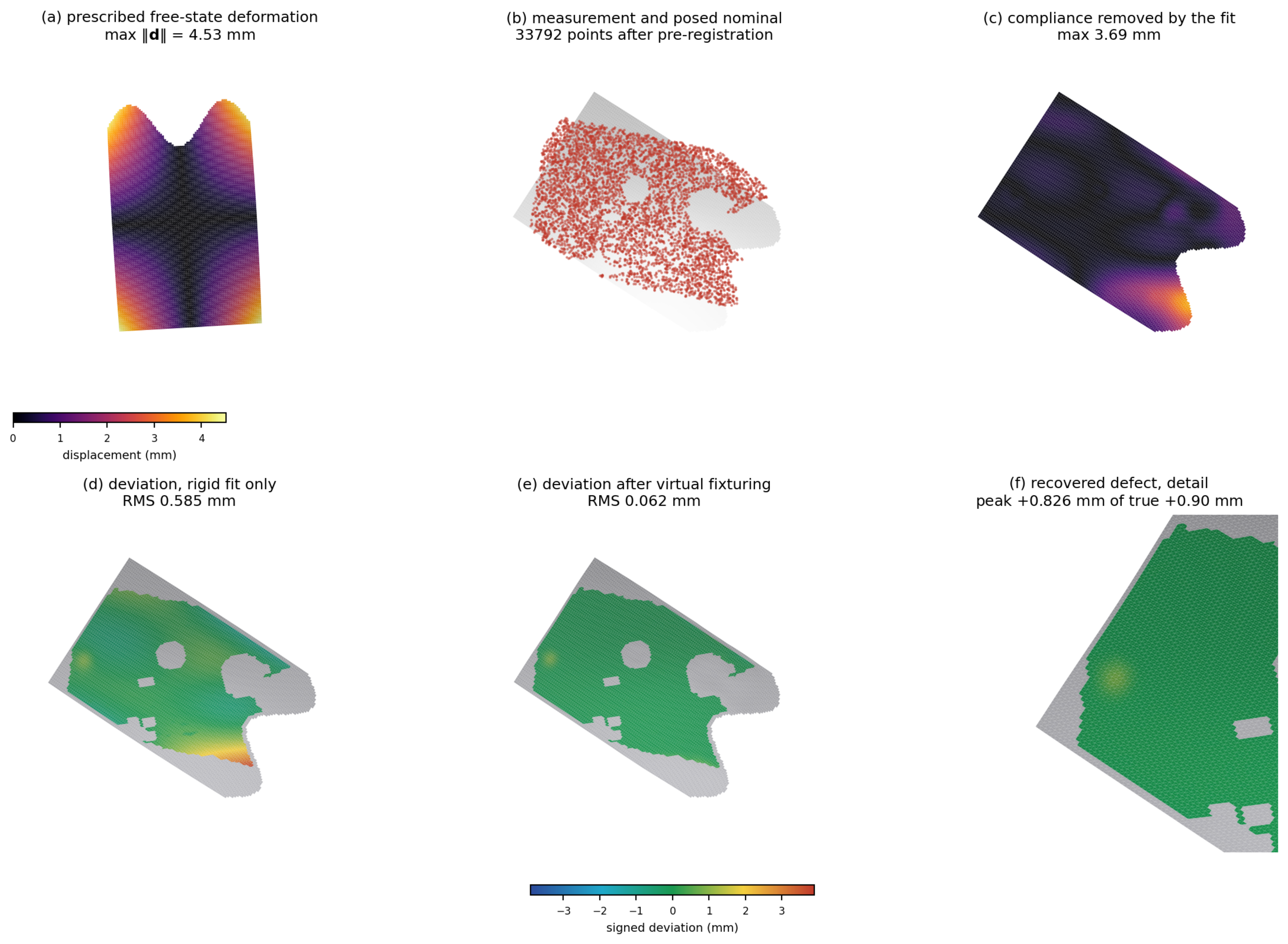
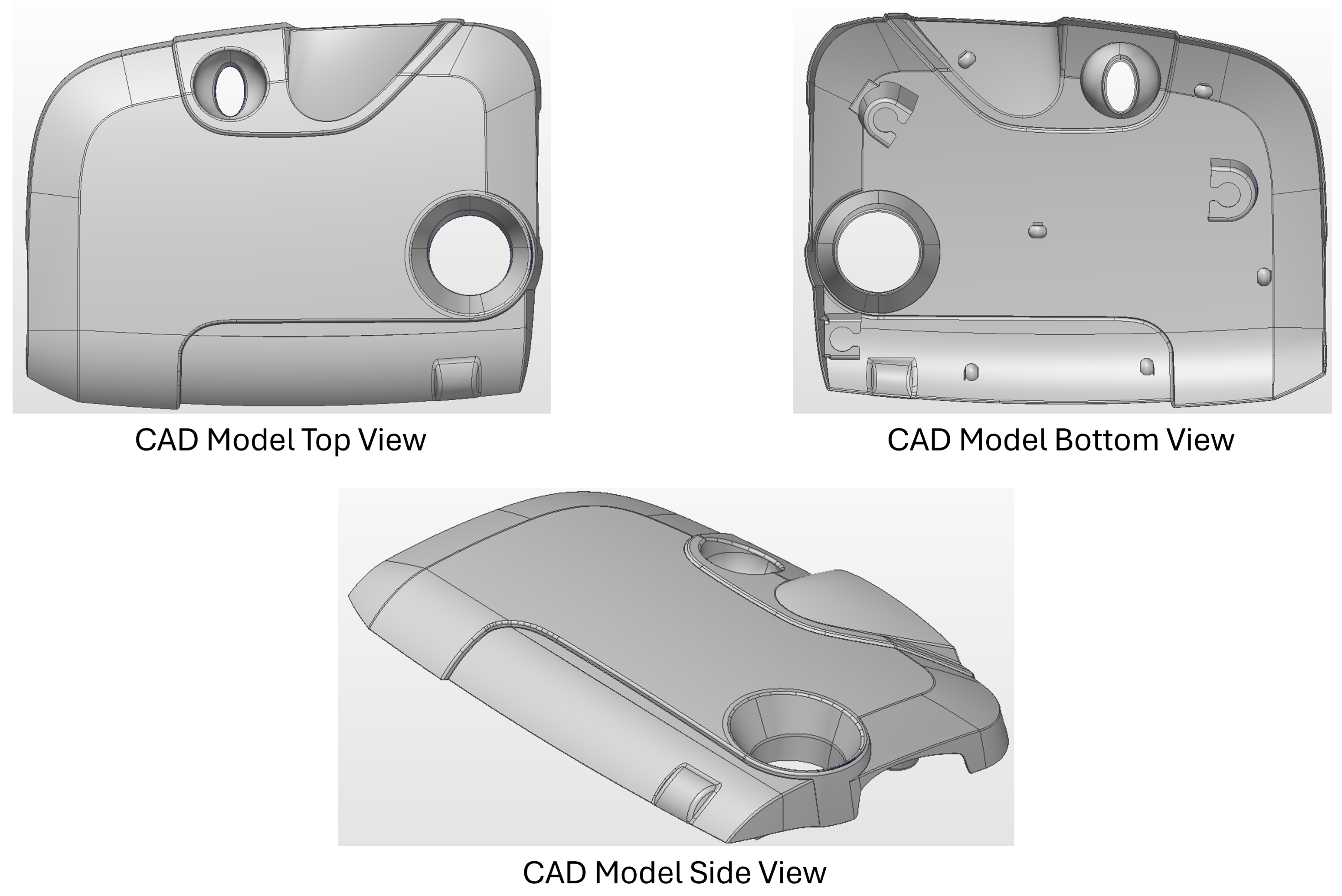
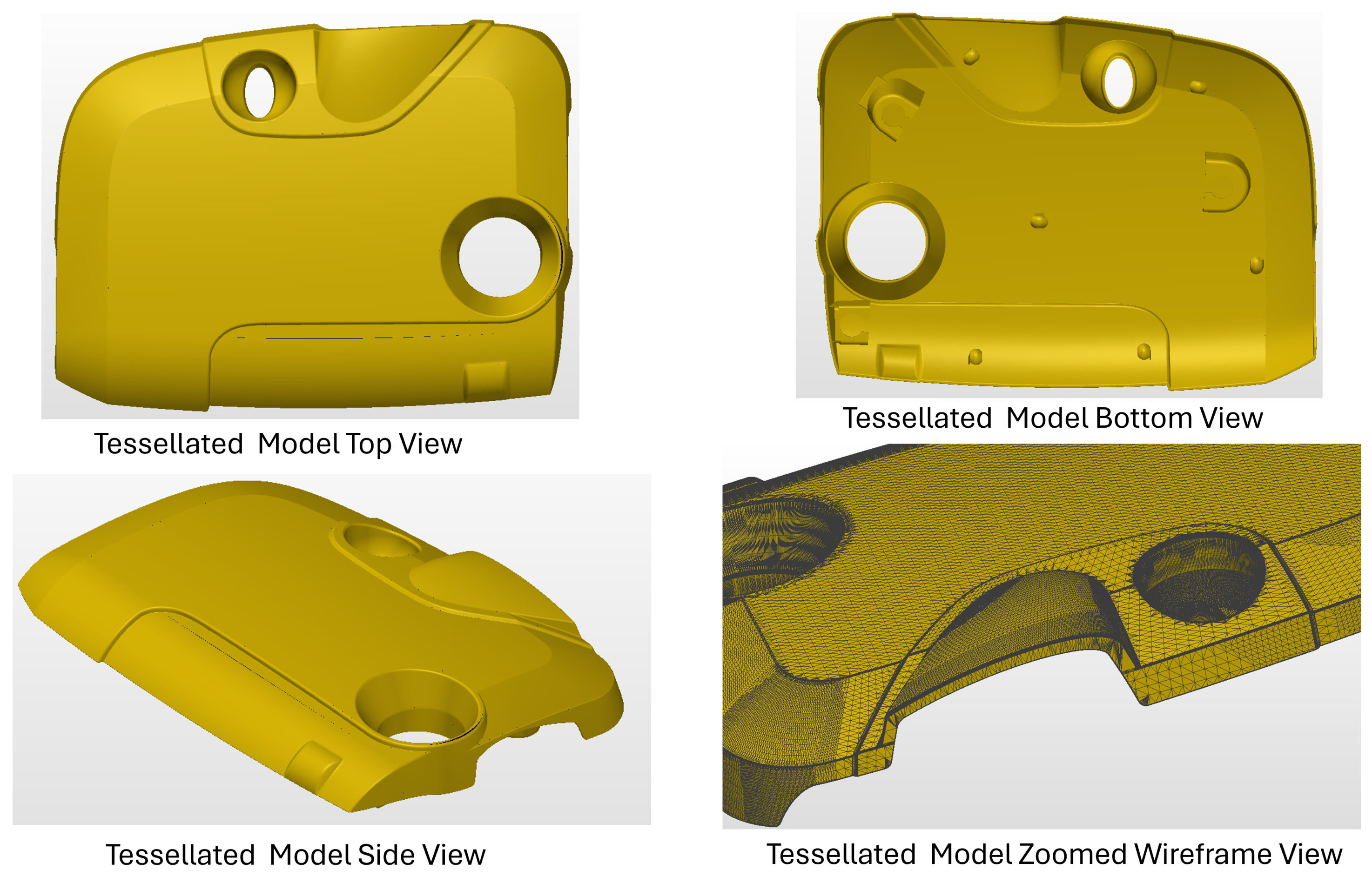
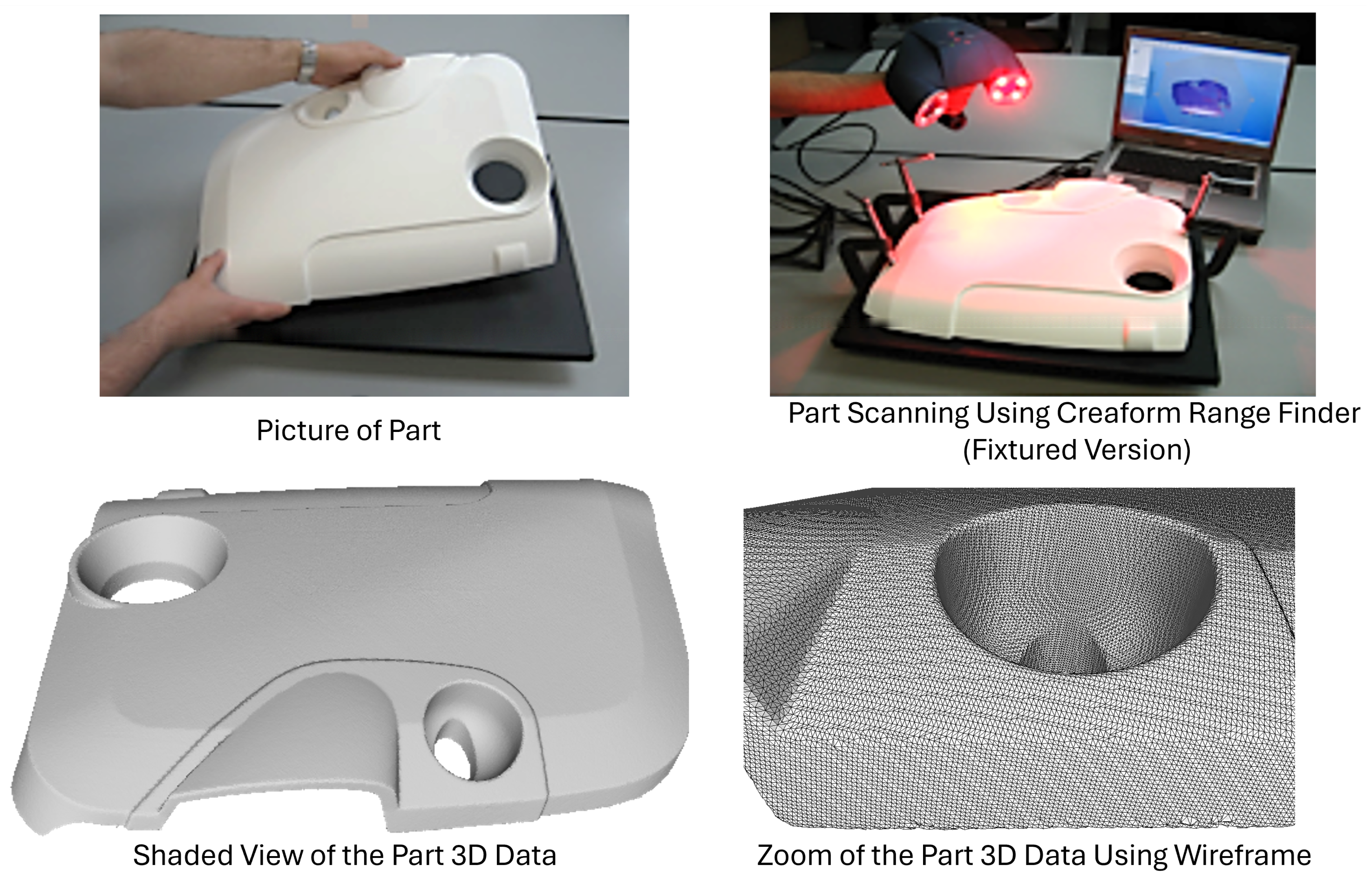
Article

Automatic Inspection of Flexible Parts Using Virtual Fixturing

Department of Computing Science, University of Alberta, 8900 114 St NW, Edmonton, AB T6G 2V4, Canada
Machines 2026, 14(9), 1057; https://doi.org/10.3390/machines14091057
Submission received: 28 July 2026 / Revised: 6 September 2026 / Accepted: 7 September 2026 / Published: 16 September 2026
(This article belongs to the Section Automation and Control Systems)

Abstract

A flexible part has no unique shape until it is constrained, which makes dimensional inspection difficult. Standard practice clamps it in a dedicated jig and probes it with a coordinate measuring machine or a range sensor. We replace the jig with virtual fixturing. From partial range views of the unfixtured part, the pipeline recovers a coarse pose between the scan and the CAD model using a robust geodesic bilateral curvature algorithm, deforms the model towards the scan by non-rigid registration, and computes deviations along the model surface normal to decide whether the part is in tolerance. On a prismatic part and a game-controller housing, the method is more accurate than optimal-step non-rigid ICP, radial basis function FEM, and coherent point drift, because the generated deformations come from an operator closely related to the proposed method’s own regularizer, those margins favor it by construction and are reported with that caveat. On a generated thin-shell test part the measurement uncertainty of the implementation is measured at about 0.039 mm, dominated by the registration rather than by the sensor. The pipeline is then exercised on a physically scanned injection-molded engine cover, a 612 mm part whose free-state residual against its nominal model is 4.62 mm at the verified global optimum. No independent coordinate-measuring-machine reference was available for that part, so this experiment is reported as a free-state residual and a controlled comparison with and without the feature set, not as a statement of absolute measurement accuracy.

1. Introduction

Dimensional inspection compares measurements of a manufactured part with its nominal CAD model and reports whether the deviations fall within the tolerance or not. For a rigid part, the procedure is well understood: the part is digitized by a 3D scanner or a coordinate measuring machine (CMM), the measured data are aligned to the model, and the residual deviations are tested against the tolerance.
In classical dimensional metrology, a manufactured part is seated in a retaining fixture that establishes the reference frame of the data set against which geometric dimensioning and tolerancing (GD&T) standards such as the ISO 1101 [1] and thebroader ISO GPS [2] system are evaluated. For a CMM, a contact touch probe is mechanically driven across the part, measuring surface points one at a time. This approach achieves micrometer-level accuracy and full traceability, which is why it remains the reference method for tight tolerancing tasks. Its limitations are speed and sparsity: it captures only tens to hundreds of discrete points rather than the entire surface, and a dedicated CMM program must be written for each new part. Because each measurement cycle is slow and must be programmed in advance, CMM inspection is poorly suited for high-throughput production lines or parts with complex and freeform geometries, where small-scale point sampling can completely miss localized defects. The reliance on physical fixturing and part-specific programming also introduces setup overhead and limits flexibility when product variants change frequently. As a result, CMM measurement is typically reserved for offline sample-based quality control rather than 100% in-line inspection, which requires the development of faster, non-contact optical, full-surface scanning techniques that trade some accuracy for dramatically higher coverage and speed.
Over the last two decades, non-contact optical range sensors have displaced the touch probe for surface inspection. Handheld structured-light and laser scanners scan the part and return a dense point cloud, hundreds of thousands of samples of the visible surface, within seconds. Modern optically tracked laser scanners reach this density at accuracies approaching those of a CMM over a working volume of a few cubic meters. The nature of the data is different in kind. A single view captures only the unoccluded, front-facing portion of the surface, so a complete scan is a set of partial range views, each a noisy sheet of points carrying occlusion gaps, dropout, and range noise, rather than a short list of exact coordinates. What the density buys is a full-field deviation map, a deviation value at every point of the visible surface rather than at a handful of probed locations, which turns inspection from point sampling into surface comparison and lets a localized defect reveal itself wherever it lies. In exchange, the burden shifts from mechanical setup to computation: the partial, noisy views must be registered to the model in software rather than aligned by a jig.
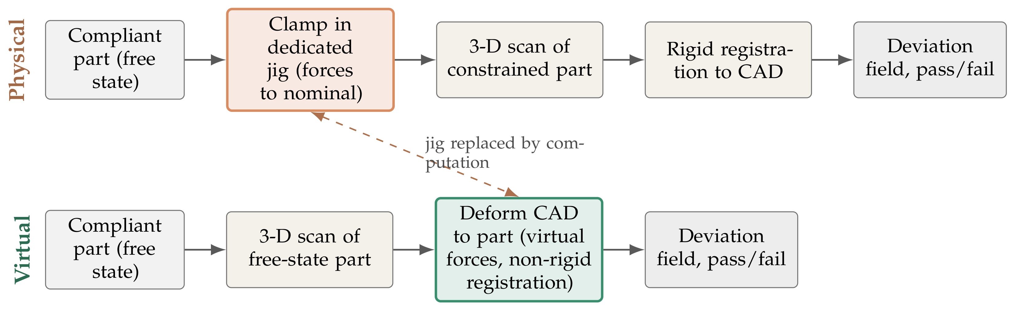
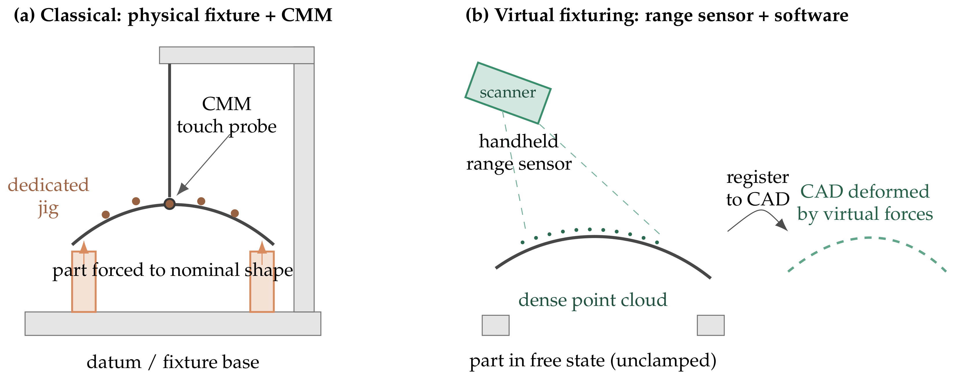
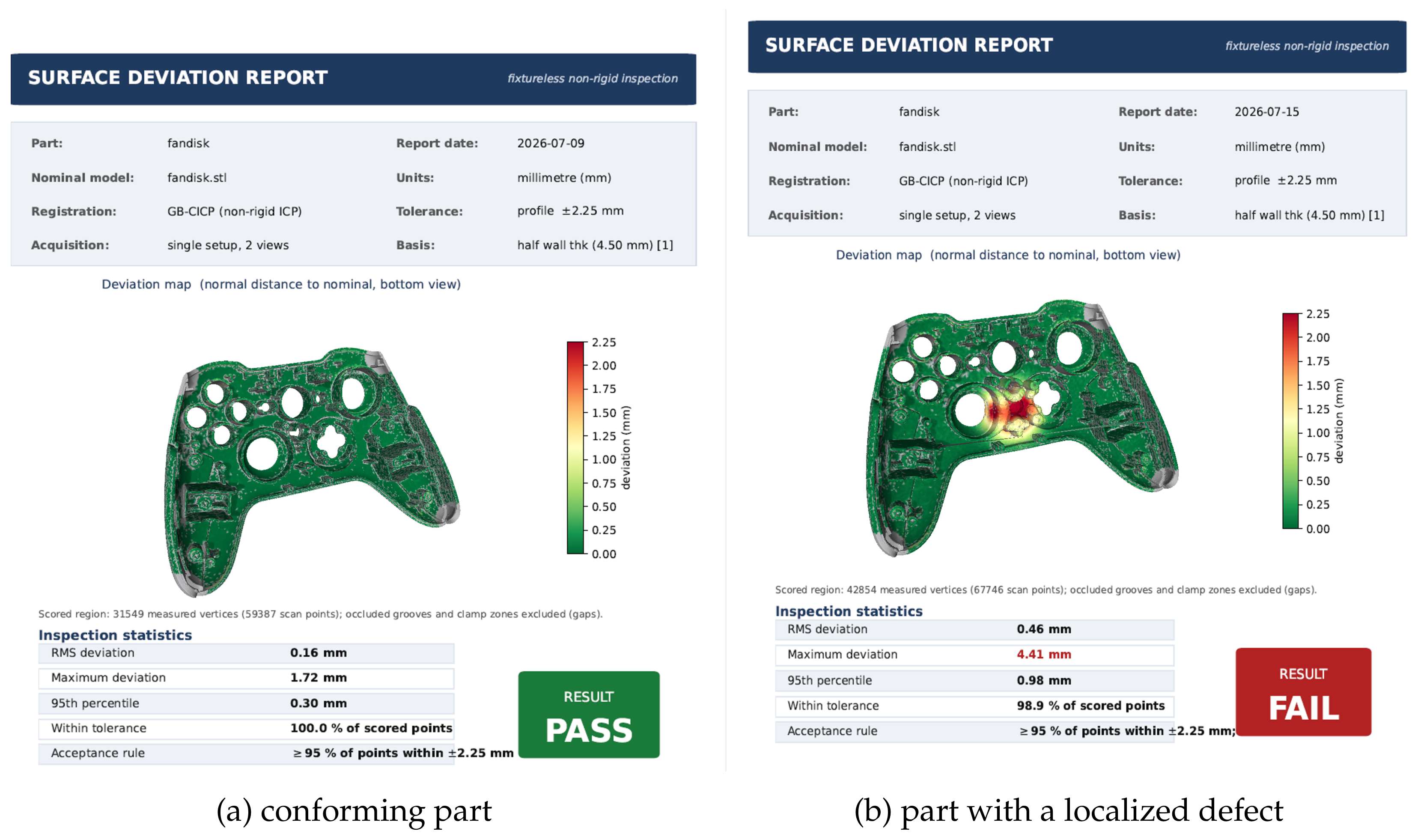
This registration step estimates the single rigid transformation ( R , t ) It is precisely this combination, speed, contact-free acquisition, and full-field coverage, that renders unfixtured scanning, and therefore virtual fixturing, practical, because the unconstrained part can now be captured quickly enough to be inspected in software rather than on a jig. Figure 1 contrasts the two arrangements.

1.1. Inspecting Non-Rigid Parts

The rigidity assumption breaks down for many industrial parts. Compliant components such as thin polymer covers and sheet-metal panels flex appreciably under their own weight or material stresses. They reach their functional shape only after they have been assembled and bolted to a neighboring structure called a jig. When such a part is measured free-standing, it will deviate from the nominal model even if it is fully within specification: the measured deviation reflects the unconstrained flexion of a conforming part rather than any manufacturing defect. A naive rigid comparison would, therefore, reject good parts and accept bad ones. At the root of the difficulty lies the fact that a compliant part has no single shape to compare against. Some criterion must first decide which of its many free-state configurations is to serve as the reference. This is precisely the problem addressed in this paper. Instead of directly comparing the measured surface with the nominal CAD model, the proposed method must first disentangle the deformation from the defect, identifying the reversible elastic flexion that even a good part exhibits in its free state.
Using a jig works, but at a cost that scales with the product mix rather than with the number of parts measured. Because the jig is specific to the part, every new component, and often every revision of an existing one, demands new tooling that must be designed, built, and certified. Mounting and releasing each part is manual and slow, limiting the process to the production line and the metrology room. The fixturing forces are themselves a source of measurement uncertainty: an over-constrained or misplaced clamp can press a defect flat or introduce a distortion that inspection then misreads as genuine form error. The upper part of Figure 2 summarizes this workflow. These drawbacks are compounded in high-mix, low-volume production, increasingly the norm in aerospace, automotive, and consumer electronics, where the fixed cost of each jig is amortized over only a handful of parts. Most fundamentally, physical fixturing conflates two roles that should remain separate: it simultaneously defines the reference configuration and physically enforces it, so any imperfection in the jig, from wear, thermal drift, or a clamp placed slightly off its contact point, propagates directly into the measurement. This coupling motivates a shift toward virtual fixturing, in which the constraining loads are applied computationally rather than mechanically, decoupling the definition of the reference shape from the physical act of holding the part.
Virtual fixturing was introduced by Jaramillo et al. [3], and the same principle underlies the generalized numerical inspection fixtures of the Tahan group [4,5]; Section 2 reviews both lines of work and their alternatives. The approach is illustrated in the lower part of Figure 2.
The trade-off migrates from hardware to computation: the fidelity of the inspection now hinges on how faithfully the deformation model reproduces the part’s true elastic behavior and on whether that deformation can be evaluated quickly enough to keep pace with production. It is precisely this tension, between physical accuracy and the speed demanded by in-line inspection, that motivates the surrogate deformation models explored in this paper.

1.2. The Deformable Registration Problem

Cast in registration terms, virtual fixturing is a non-rigid registration of the CAD model to the scan, regularized so that the recovered deformation is physically plausible. This means that the model may bend as a real compliant part would but cannot stretch or fold in ways that would mask a genuine defect. Once the model has been brought onto the scan reference, everything downstream, the deviation map, and the pass-or-fail decision follow exactly as in the rigid case. The entire difficulty is therefore concentrated in the deformable registration procedure itself. The open question it raises is a precise one: which registration algorithm recovers the free-state surface faithfully enough to be able to inspect, given only the partial, noisy range views that a real sensor returns. Also, is the algorithm able to recover the original part surface accurately enough to perform the inspection? These two objectives are not obviously the same. An algorithm may reconstruct the overall surface with low average error yet smooth over the very local features that signal a defect, while another may track the surface less faithfully in aggregate but preserve the sharp residuals that inspection depends upon. Distinguishing these behaviors is exactly what a rigorous inspection must expose.
We resolve this by making the deformation the output of a physical model. Instead of directly defining an artificial displacement field, we define virtual loads and boundary conditions on the nominal CAD such as support points, gravity, and forces at the application points, and then solve the resulting elastostatic equilibrium. The deformed surface is then known exactly because we computed it, but physically admissible by construction because it satisfies equilibrium, compatibility, and the constitutive law. In practice, the free states are drawn from the part’s lowest elastic modes, which span exactly the flexure a compliant part exhibits while remaining cheap to sample, and a separately prescribed local defect is superimposed on this physical deformation so that reconstruction accuracy and defect detectability can be scored independently against the same known reference. One property of this design must be stated at the outset rather than left to the reader to notice. The generator’s intrinsic operator is closely related to the smoothness prior that GB–CICP uses as its regularizer, so on generated data the proposed method’s prior matches the data-generating process, while its competitors’ priors do not. Any margin GB–CICP shows on such data is therefore partly a property of the experimental design rather than of the algorithm. We mitigate this in three ways: the concern is restated at the point of comparison in Section 8.1; the physically scanned part of Section 8.4, whose compliance is imposed by gravity and free-state handling, is deformed by no operator we chose and is accordingly treated as the arbiter of the comparison; and the released generator accepts alternative deformation models so that the ranking can be retested against a prior unrelated to any competitor’s, which we identify in Section 11 as required future work.

1.3. Paper Organization

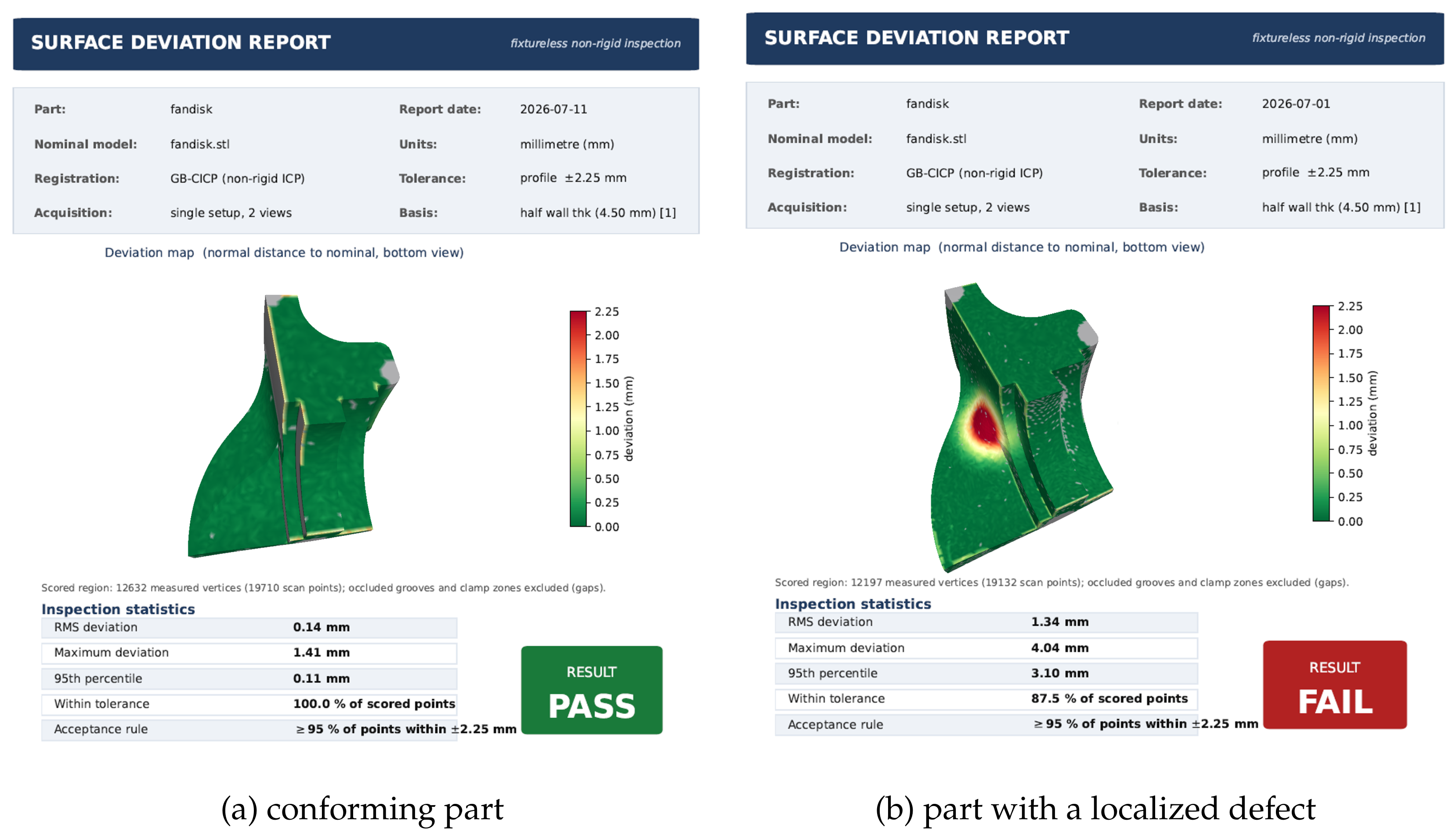
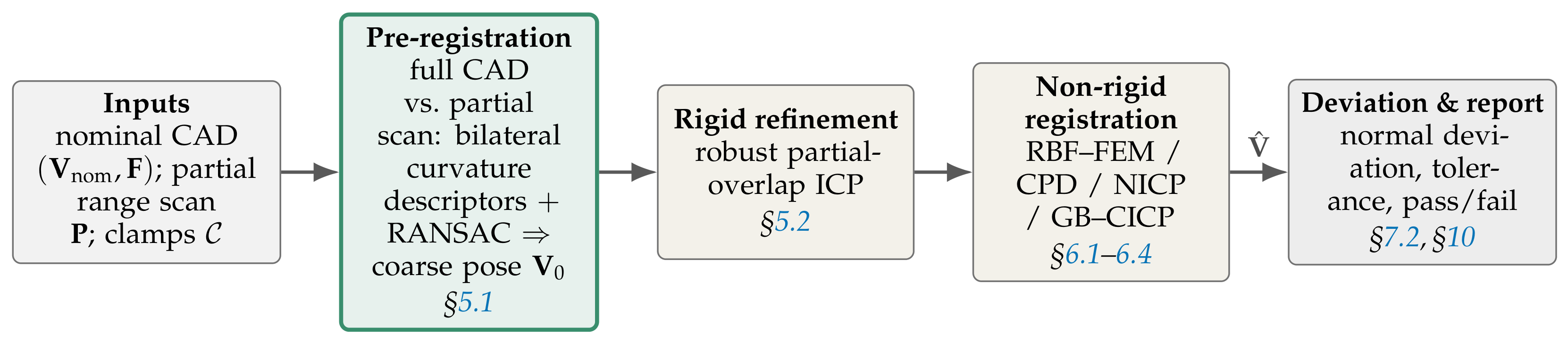
In this framework, the paper describes the inspection process from end to end and examines the registration on which it rests. Beginning from a partial, noisy range view of the free-state part, a coarse pose is first recovered by matching the complete undeformed CAD model to the scan using a novel geodesic bilateral curvature descriptors algorithm (Section 5.1). Based on this initial registration, a non-rigid registration algorithm then deforms the model onto the scan, and the residual is scored as a point-to-surface deviation against a tolerance derived from the part’s wall thickness, or from its bounding-box diagonal where no single thickness is defined. Applying the 95% in-tolerance pass combined with a maximum deviation threshold rules, a pass-or-fail conformance report can be determined (Section 7.2 and Section 10). For the deforming step, the study compares four registration algorithms of increasing freedom: the RBF–FEM seed method, coherent point drift, non-rigid optimal-step ICP, and a geodesic biharmonic curvature variant of non-rigid ICP on identical parts, scans, and scoring rule (Section 3, Section 4, Section 5, Section 6, Section 7 and Section 8).
That comparison is carried out on generated scans of two CAD models, which is what makes the exact ground truth available. Generated data alone cannot settle the question, however, for two reasons: the deformations are produced by an operator related to the proposed method’s own regularizer, so the comparison is not neutral between the candidates, and a generated mesh cannot reproduce the conditions a real acquisition imposes. The evaluation therefore closes on a physically scanned part. Section 8.4 carries the identical pipeline, without modifications, through an injection-molded automotive engine cover digitized in the free state with a commercial hand-held range sensor, whose compliance is imposed by gravity rather than by any prior we chose, and reports both the deviation field on the part as manufactured and a controlled comparison in which known material is added while the nominal, the pose, and the processing are held fixed. Section 8.3 then quantifies the limit of what can be detected as a function of the amplitude and width of the defect, and Section 9 gives an uncertainty analysis for the deviation field in which the registration, not the sensor, is the dominant term. Two CAD models are used for that comparison, and because their deformations are generated by an operator related to the proposed method’s own regularizer, the complete process is then run without retuning on a physically scanned part, an injection-molded automotive engine cover digitized in the free state with a commercial hand-held range sensor, whose compliance is imposed by gravity rather than by any prior we chose (Section 8.4). Section 8.3 quantifies the defects the process can and cannot resolve as a function of their amplitude and width, and Section 9 gives an uncertainty budget for the deviation field in which the registration, not the sensor, is the dominant term.

2. Background and Related Work

This section reviews the literature relevant to the proposed algorithm. The organizing thread is the inspection problem: we first trace how dimensional inspection has been formulated for rigid parts and then extended to flexible ones, identifying the open question, which registration algorithm a fixtureless inspection process should adopt. We then review the registration and deformation techniques from which the proposed inspection methods are based and close with the discrete operators and sensor models that allow those candidates to be evaluated against exact ground truth on generated data, before the process is taken to a physically scanned part where no such ground truth exists.

2.1. Dimensional Inspection and the Rigid Assumption

Dimensional inspection compares a measured surface with a nominal CAD model and reports whether the deviations between them fall within tolerance. As mentioned previously, when the part is rigid, the alignment is a single rigid motion of six degrees of freedom, and the literature on freeform inspection is organized almost entirely around this case. A review of freeform surface inspection techniques is presented in Li and Gu [6] and a survey of freeform metrology by Savio et al., De Chiffre, and Schmitt [7] both structure the problem in the same way: acquire the surface, fit it rigidly to the nominal model, and read the deviation, with methodological attention falling on the acquisition and the fitting rather than on the assumption they share. Advances in instrumentation have broadened the range of data entering this pipeline. The multi-sensor data fusion reviewed by Weckenmann et al. [8] combines tactile, optical, and computed-tomography measurements into a single richer representation of the surface. Richer data, however, do not change the logic of the comparison: regardless of the sensor, the alignment step still presumes that the part possesses one nominal shape to be aligned to, so that any residual after alignment can be attributed to manufacturing error.

2.2. Inspection of Flexible and Non-Rigid Parts

A distinct subfield of inspection explicitly treats deformation along two main strategies. The first compensates for distortion by simulating the constraining forces. Weckenmann et al. applied virtual forces to a finite element (FEM) model built from the measured sheet-metal surface [9], and Gentilini and Shimada predicted the post-assembly shape by combining laser digitization with an FEM simulation of the assembly process [10]. Both require digitizing essentially the whole deformed surface to work. The second strategy avoids physical fixturing altogether. Abenhaim and colleagues introduced an approach for inspecting flexible parts without special fixtures [11], and the generalized numerical inspection fixture of Radvar-Esfahlan and Tahan replaced the jig with a geometric computational constraint [4]. This approach has continued to develop, for instance, with robustness and rectification procedures for fixtureless inspection of non-rigid parts [5]. The challenges, notions, and state of the art of the non-rigid inspection problem are surveyed by Abenhaim et al. [12]. The work of ref. [3] belongs to the force-simulation family, but inverts the data requirement of ref. [9]. It deforms the CAD model rather than a measured surface, requires only clamping regions, and approximates the FEM solution with a field of radial basis functions for speed. A companion study extended the idea to inspection from partial views [13]. What none of these works provides is a registration step scored against a known free-state surface, so it remains hard to say which registration algorithm an inspection process should adopt. This gap frames the review of the registration methods that follows.

2.3. Rigid Registration Algorithms

Every inspection pipeline, rigid or not, must perform a rigid registration step, at least as initialization. The step originates from the iterative closest point (ICP) algorithm [14,15,16], which alternates closest point correspondence with a rigid fit and which the Chen and Medioni algorithm recasts in point-to-plane form for faster convergence [15]. Practical variants and their convergence and sampling tradeoffs are cataloged by Rusinkiewicz and Levoy [17], and probabilistic and globally optimal formulations were generalized by [18] and Go-ICP [19]. Because the closest-point ICP requires a good initial pose, feature-based and global methods such as fast point feature histograms [20] and fast global registration [21] are used to fully automate the registration process.

2.4. Non-Rigid Registration Algorithms

For a deformable part, the residual after the initial rigid alignment is itself a deformation field, so the rigid fit must be replaced by a regularized non-rigid one. This is the component on which the fixtureless inspection of flexible parts ultimately rests. Probabilistic point-set methods include the robust thin-plate-spline point matching of Chui and Rangarajan [22] and the coherent point drift of Myronenko and Song [23]. Surface-based methods include optimal-step non-rigid ICP [24], template fitting to range scans [25], global correspondence optimization [26], and global non-rigid alignment of multiple scans [27]. The survey by Tam et al. presents the evolution of the algorithms from rigid to non-rigid registration [28].

2.5. Recent Learning-Based and Deformable Registration

In recent years, registration has been dominated by learning-based algorithms, although few have been assessed in a metrology setting. The early pipelines combined point representations [29] with end-to-end alignment, as in PointNetLK [30] and the deep closest point [31], and with learned local descriptors such as fully convolutional geometric features [32] and D3Feat [33]. Robustness to outliers and partial overlap was addressed by RPM-Net [34], deep global registration [35], PREDATOR for low-overlap pairs [36], and transformer matchers including GeoTransformer [37] and REGTR [38]. The area was comprehensively surveyed by Guo et al. [39], these algorithms largely assume rigidity. The deformable case has only recently received comparable attention: Lepard learns partial matching for both rigid and deformable scenes and introduced the 4DMatch benchmark [40], the neural deformation pyramid performs non-rigid registration per pair without training data [41], and transformer formulations have been applied directly to non-rigid shape registration [42].

2.6. Surface Deformation and Variational Methods

The deformation prior that a non-rigid inspection method imposes, and the deformations against which it must be tested, come from variational surface modeling. The Laplacian surface editing [43], as-rigid as-possible modeling [44], and embedded deformation graphs [45] span the nonlinear end, while the linear methods that obtain a smooth displacement by minimizing a quadratic bending energy are surveyed by Botsch and Sorkine [46]. The bounded biharmonic weights of Jacobson et al. [47] are a direct relative of the proposed algorithm.

2.7. Discrete Operators and Geodesic Methods

The operators underlying both our deformation and our curvature-aware registration algorithm are classical. The cotangent Laplacian originates with Pinkall and Polthier [48], discrete differential-geometry operators for curvature and area on triangle meshes are consolidated by Meyer et al. [49], and the standard treatment of these tools is the polygon mesh processing literature [50]. The intrinsic geodesic viewpoint that motivates the curvature-compatible correspondence weighting connects to the exact and approximate geodesic computation on the meshes [51,52] and to the heat method for geodesic distance [53]. The same intrinsic philosophy underlies the functional map framework for shape correspondence [54] and its learned descendants [55], which represent maps on the Laplace–Beltrami eigen-basis and are most effective in quasi-isometric deformations produced by thin-plate bending.

2.8. Three-Dimensional Sensor Modeling

Evaluating inspection methods based on simulation requires a model that simulates the behavior of real range data sensors. The range sensing technology and its two decades of development are reviewed by Blais [56]. Structured-light acquisition, the dominant modality for the parts considered here, is surveyed in the tutorials by Salvi et al. [57] and Geng [58]. The volumetric image-range integration of Curless and Levoy [59] established the partial-view multi-scan setting that our scanner model reproduces, including self-occlusion and missing data.

3. Defining the Virtual Fixturing Inspection Pipeline

Given the nominal CAD mesh ( V nom , F ) with n vertices, a multi-view registered measurement point cloud P = { p k } k = 1 m , and the indices C of the clamping vertices, the task is to produce an estimated deformed surface V ^ R n × 3 expressed in the nominal vertex set. Virtual fixturing computes V ^ under two competing requirements: the estimate must fit the measured scan, while the deformation carrying V nom to V ^ must remain physically plausible. Plausibility means that the surface may bend as a real compliant part would under its support and clamping loads, but may not stretch, shear, or fold in ways that no elastic body would sustain. This second requirement is what keeps the estimate from merely interpolating measurement noise or absorbing a genuine manufacturing defect into the deformation field, and it is precisely the constraint that each algorithm encodes through its physical deformation prior.
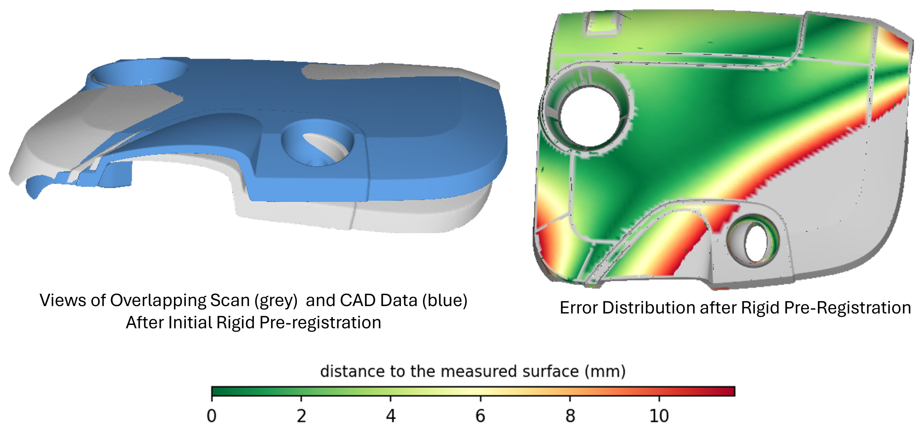
However, before any deformation can be applied to the CAD model, the measured data and the model must share a common reference frame. Establishing it is the role of the pre-registration stage, which proceeds in two steps. The first assembles the point cloud: the tracked scanner of Section 4 places every swath directly in the tracker frame, so the views accumulate into a single coordinate system without scan-to-scan alignment. The result is a point cloud P , in a common frame, covering the visible part. Since the part is placed freely in the scanner volume, P initially lies at an arbitrary rotation and translation with respect to V nom . A global initial alignment followed by rigid ICP refinement estimates the six-degree-of-freedom transform that best fits the cloud to the nominal mesh, and this transform is applied to P once and for all. This initial registration removes the unknown placement of the part relative to the model, but no rigid motion can account for the compliant free-state deformation itself. The misfit remaining after rigid alignment is therefore exactly the signal the non-rigid stage uses.
The four deformable registration algorithms studied in this paper differ only in how strongly and through which mechanisms they enforce physical plausibility. Crucially, the four non-rigid methods are all initialized from the samerigid pre-registration, so that the comparison isolates the deformation prior rather than the pose search: any difference in the recovered V ^ is attributable to the prior alone, not to a better or worse starting pose. Figure 3 traces the data-processing stages from beginning to end.

4. Multiview Part Digitization and Deformation Modeling

This section sets out the two ingredients on which the inspection process relies: how the part is digitized and how its deformed free state is generated. We first describe the physical data acquisition we emulate, an optically tracked handheld laser scanner that sweeps the part and returns a single registered point cloud, and then the simulator that reproduces it. Rather than measuring real parts, we simulate the data acquisition process using an orthographic sweep with a depth buffer, a grazing-angle cutoff, range noise, and dropout at the clamps, so that each virtual view carries the same partial coverage, self-occlusion, noise, and missing data a real handheld sensor introduces. This simulated acquisition is driven by a deformation model, described in the second half, that turns the nominal CAD mesh into a smooth, physically plausible free-state surface with exactly known ground truth. The two form one pipeline: the deformation model prescribes the truth, and the simulated scanner produces a realistic observation of it, together defining the input P and the reference surface against which every registration algorithm of Section 5 and Section 6 is scored.

4.1. Multiview Digitization Using Real Range Sensors

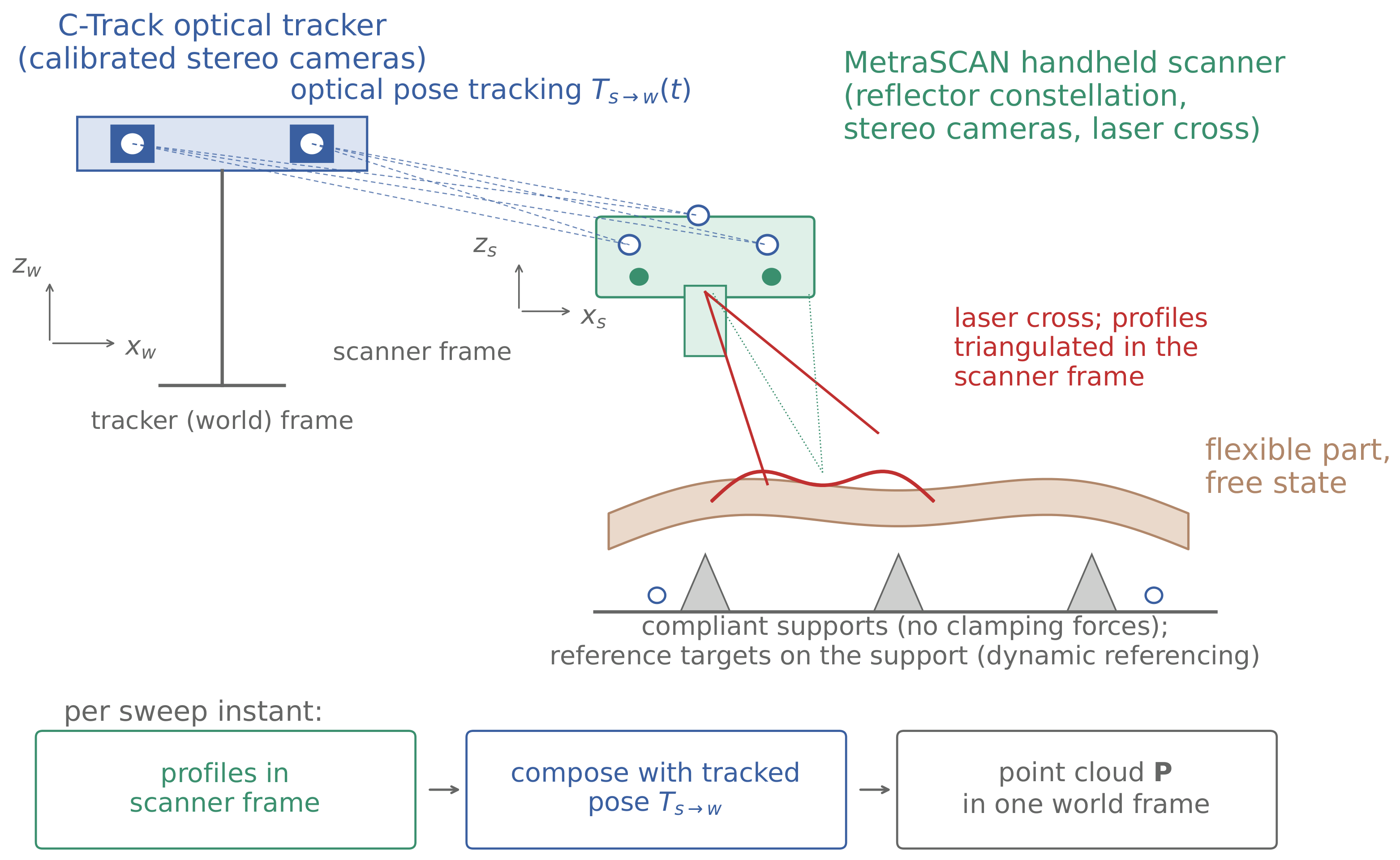
The inspection process shown in Figure 3 starts with scanning the freeform part’s surface with an optically tracked handheld laser scanner. Handheld scanners establish their own pose in one of two ways. Self-positioning scanners, such as the Creaform HandySCAN family, triangulate their pose from retro-reflective targets that must first be applied to the part or to a frame around it. For obvious reasons, this type of scanner is not very practical for online inspection. Optically tracked scanners, such as the Creaform MetraSCAN paired with its C-Track optical tracker, invert the arrangement: a fixed stereo tracker continuously observes a constellation of reflectors mounted on the scanner body itself, so the scanner pose is known in the tracker frame at every instant, and the part carries no targets at all. The arrangement is not unique to Creaform. Nikon’s K-series optical CMM TRACK light-emitting diodes mounted on its ModelMaker handheld laser scanners; the ZEISS T-SCAN, originating from Steinbichler, is tracked by the T-TRACK stereo tracker; and Hexagon pairs a Leica laser tracker with a handheld scanner, the same principle as an interferometric tracker and a camera-based orientation unit in place of the stereo pair. Articulated measurement arms such as the FARO and Hexagon scanning arms achieve the same target-free referencing mechanically, at the price of tethering the scanner to the arm’s reach. For a flexible part, this target-free operation is important, since applying and pressing targets onto a compliant surface loads exactly the geometry one is trying to measure in its free state.
Capturing the surface of the part then proceeds by sweeping, as sketched in Figure 4. The scanner projects a set of laser lines onto the surface. Its onboard cameras triangulate the illuminated profiles in the scanner frame, and the tracker pose, composed of each profile, places the points directly in a single world frame. Sweeping the scanner over the part accumulates overlapping swaths that are natively expressed in that common frame, so the multiple views of our sensor model arrive already mutually registered, and no scan-to-scan alignment is needed. The part rests in its free state on compliant supports. If the part or its support can move during the sweep, reference targets placed on the support rather than on the part let the tracker compensate for the rigid motion, a mode the manufacturer calls dynamic referencing. The operator sweeps until the inspected face is covered, which is exactly the ring of viewpoints the simulator of Section 4.2 synthesizes, and the same artifacts appear for the same reasons: no data behind occlusions, weak return at grazing incidence and on shiny surfaces, and dropout where the supports contact the part.
The output of such a session is an unordered point cloud in the tracker frame, which is precisely the input P that our pipeline assumes. The tracker frame bears no relation to the CAD frame, which is why the process begins with the descriptor-based pre-registration of Section 5.1 rather than with an assumed initial pose, and everything downstream, the non-rigid registration and the conformance report, is unchanged whether P came from the virtual scanner or from a tracked laser scanner.
The accuracy of such a system is worth examining because it decomposes in a way that maps directly onto the dataset’s noise model. Three contributions stack. The first is the accuracy of the scanner head itself, the laser-triangulated profile points in the scanner frame, which for current Creaform metrology-grade heads is stated by the manufacturer at the level of a few hundredths of a millimeter. The second is the pose error of the optical tracker, which enters every point through the composed transformation and grows with the tracker-to-scanner distance. For this reason the tracked combination is specified not by a single number but by a volumetric accuracy over a stated working volume, and the manufacturer’s figures for the MetraSCAN and C-Track pair keep this combined error below roughly a tenth of a millimeter over working volumes of several cubic meters, under acceptance procedures in the spirit of VDI/VDE 2634. The third is the measurement itself: calibration state, surface finish and color, incidence angle, and ambient conditions, all of which move the realized accuracy away from the datasheet value, which is why current data sheets should be consulted for any specific configuration rather than figures repeated here. The important structural point is that the error budget of a tracked scanner is dominated by a smooth, slowly varying pose component plus a per-point triangulation noise, and it is the second of these that limits inspection of a single part standing well inside the tracking volume.

4.2. Simulating Multiview Range Sensing

The strategy of prescribing ground truth and synthesizing the observation, rather than measuring a real scene with range sensors and labeling it, is well established in places where exact labels are otherwise unobtainable. Synthetic imagery has trained and evaluated optical-flow estimators and scene-flow estimators [60], and synthetic trajectories underlie RGB-D reconstruction and SLAM benchmarks [61]. For shape, large model repositories such as ModelNet [62] and ShapeNet [63] provide clean geometry, and the FAUST dataset provides paired meshes with exact correspondence specifically to evaluate registration [64]. Our evaluation applies the same principle to a manufacturing problem where paired scan and deformation data do not exist: it prescribes the deformation field and synthesizes the scan, so that registration accuracy becomes directly measurable.
Our simulator is designed to reproduce the four artifacts that matter for fixtureless inspection, partial coverage, self-occlusion, range noise, and missing data at the clamps, so that the views a registration algorithm sees carry the same difficulties a real handheld sensor would introduce. For each acquisition point of view v k , the surface is projected orthographically along v k onto an image grid, and a depth buffer retains only the nearest sample per pixel, which removes the self-occluded surface. A grazing-angle cutoff then discards vertices whose normal is nearly perpendicular to the view direction, | n i · v ^ k | < τ g , since a real scanner returns little signal at the grazing incidence. Each retained sample is perturbed by Gaussian range noise along the view direction,
p = x + η v ^ k , η N ( 0 , σ 2 ) ,
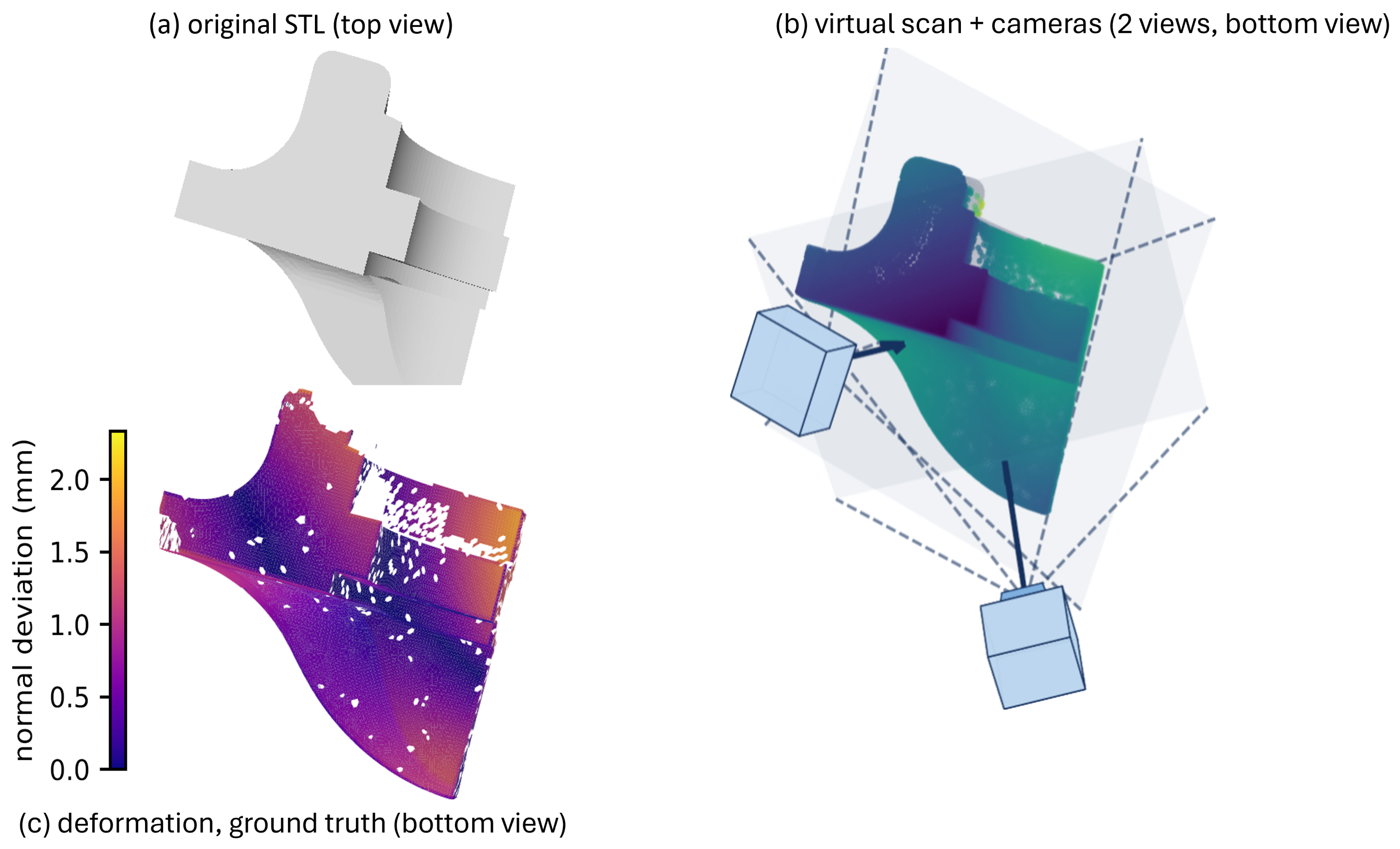
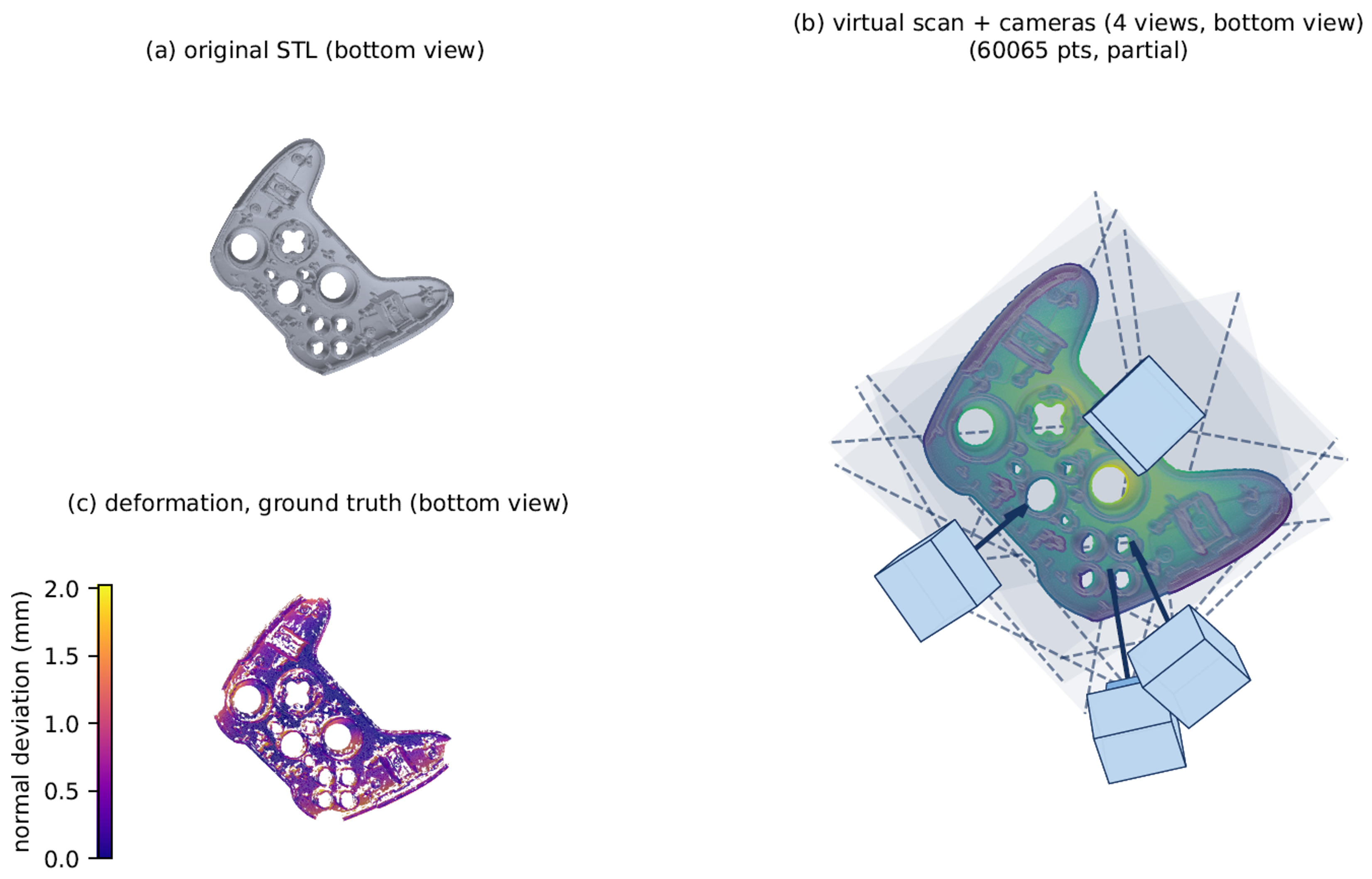
at one of the three noise levels σ . Random thinning then removes a fraction of the points to model dropout, and an additional dropout disk of fixed radius around each clamp reproduces the missing-data regions that appear around force-application points in real measurements. The points from all views are concatenated into a single unordered cloud. For every measured point, we record the index of the vertex from which it originated. This generator correspondence is used only to define the inspected (measured) vertex set and to score accuracy and is never passed to a registration algorithm. Figure 5 shows the acquisition geometry on a real STL part: panel (a) is the nominal CAD surface, panel (b) a two-view scan together with a virtual camera and its view frustum in each acquisition pose, and panel (c) the prescribed deformation retained as the exact ground truth.
Figure 5. The generator pipeline on the fandisk CAD model, shown in bottom view throughout. (a) The original STL as CAD reference, shaded. (b) A virtual scan from two viewpoints, each acquisition viewpoint marked by its virtual camera and view frustum, returning a partial point cloud over the surface visible to the cameras. (c) A prescribed deformation applied to the part and kept as exact ground truth, colored by normal deviation. The recovered inspection deviation for this case is reported in Figure 6.
Machines 14 01057 g005
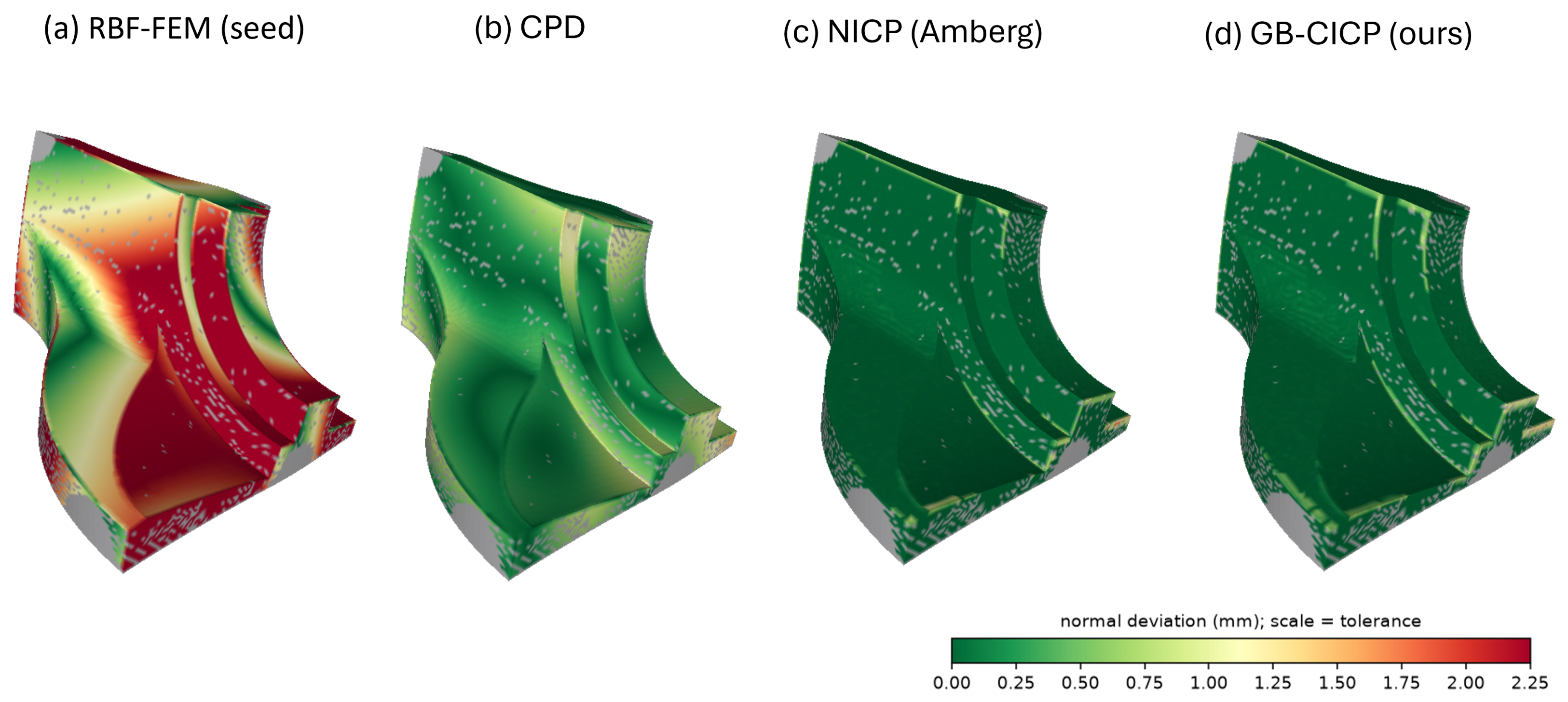
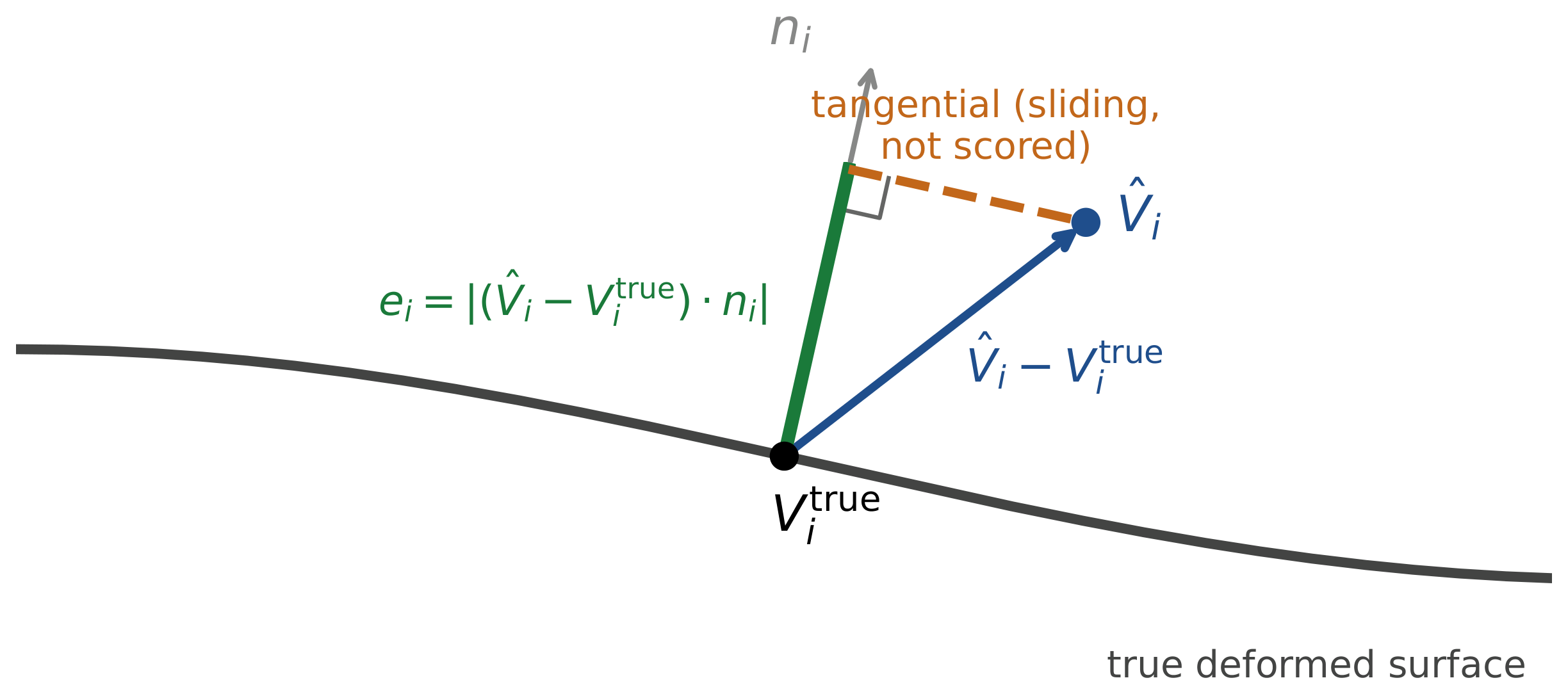
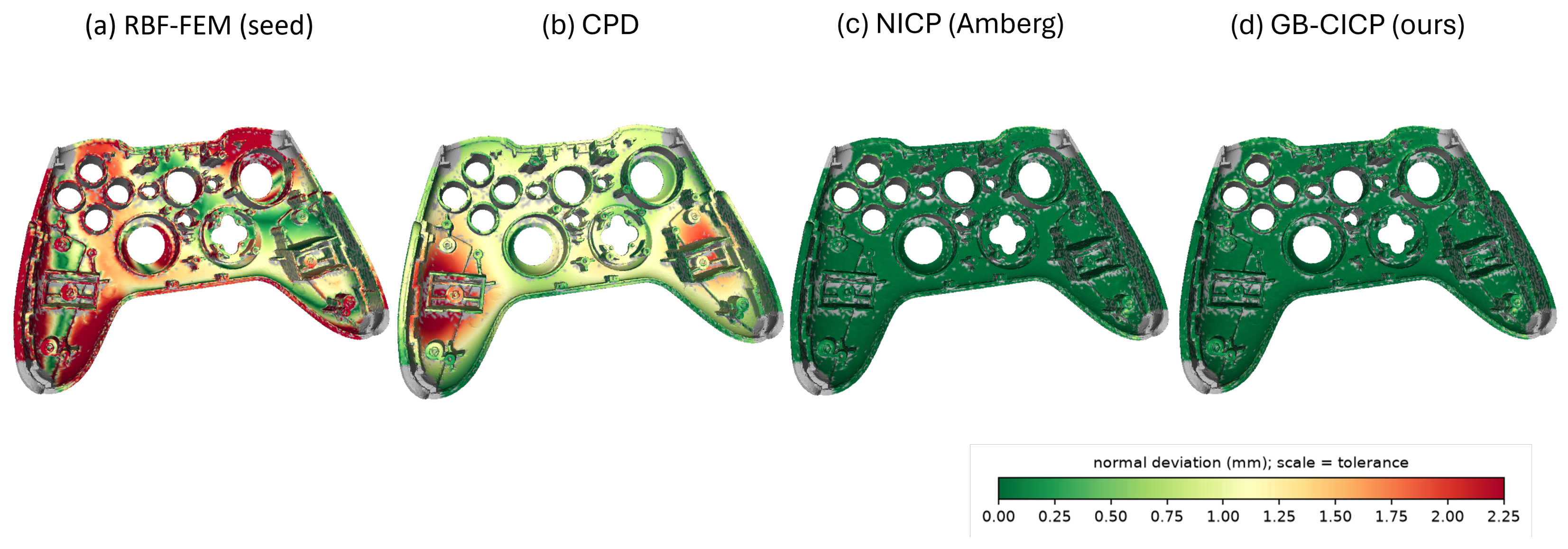
Figure 6. The four entrants on the fandisk worked example of Section 7.1 (the part of Figure 5). Because the scan is a one-sided surface, deviation is measured along the surface normal—the quantity a deviation report uses—so tangential sliding, which leaves the surface in place and which no point-based method can observe, is correctly excluded. GB–CICP (0.12 mm RMS) and NICP (0.14 mm) recover the surface almost exactly; CPD (0.47 mm) leaves visible residual; and RBF–FEM, starved by the data deliberately missing at the clamps, fails outright (2.56 mm RMS, 7.19 mm maximum). Only the vertices the scanner measured are scored, so the occluded groove interiors and the clamp regions appear as gaps rather than as spurious deviation.
Machines 14 01057 g006
Simulating acquisition, rather than scanning physical parts, is what makes evaluation possible, and it is preferable here for four reasons. The most important one is ground truth: the central quantity this study measures is how far a recovered surface lies from the true free-state shape, and on a physically scanned part that shape is unknown, as one could only compare a scan against another scan, never against a number. Because the simulator produces the free-state surface and the range view of it together, every point carries an exact reference and an exact generator correspondence, so the accuracy becomes a measured quantity instead of a visual impression. Second, control: the artifacts that most stress fixtureless registration such as noise amplitude, the number and placement of viewpoints, the degree of thinning, and the size of the clamp dropout. These parameters can be dialed to prescribed levels and swept independently, isolating the effect of each, whereas a physical rig couples them and fixes them at whatever the hardware happens to deliver. Third, neutrality and reproducibility: a real acquisition would bind the results to one sensor’s resolution, optics, and noise signature, undermining exactly the scanner-agnostic claim we seek. A parametric simulator instead spans a family of sensing conditions and lets any reader regenerate the identical dataset without access to our hardware or parts. Fourth, scale and cost: obtaining hundreds of deformed specimens with metrology-grade ground truth would require fabricating, deforming, and reference-measuring each one on a CMM, an effort that does not scale. The simulator generates a statistically large and balanced dataset at negligible cost. The trade-off is fidelity, as a simulator can only reproduce the artifacts it models, which is why we deliberately inject the four that dominate fixtureless scanning and validate the acquisition geometry against a real STL part in Figure 5, so that the synthetic views remain representative of the measurements that the process would face in practice.

4.3. How to Simulate a Deformed Free-State Surface

The virtual scanner described in the previous section does not measure the nominal CAD model but its freely deformed counterpart after manufacturing. Before any acquisition can be simulated, we must therefore decide what that deformed surface is. The scanner is, in essence, a map that takes a shape as input and returns a partial, noisy view of it. The shape it digitizes is the free-state configuration that a compliant part assumes once released from its fixture. For this deformation to be physically plausible, it must be smooth and introduce a low distortion. The generator and the scanner thus form two stages of a single pipeline: the deformation model turns the nominal STL model into a plausible free-state surface with exactly known ground truth, and the scanner then samples that deformed surface under realistic sensing conditions.
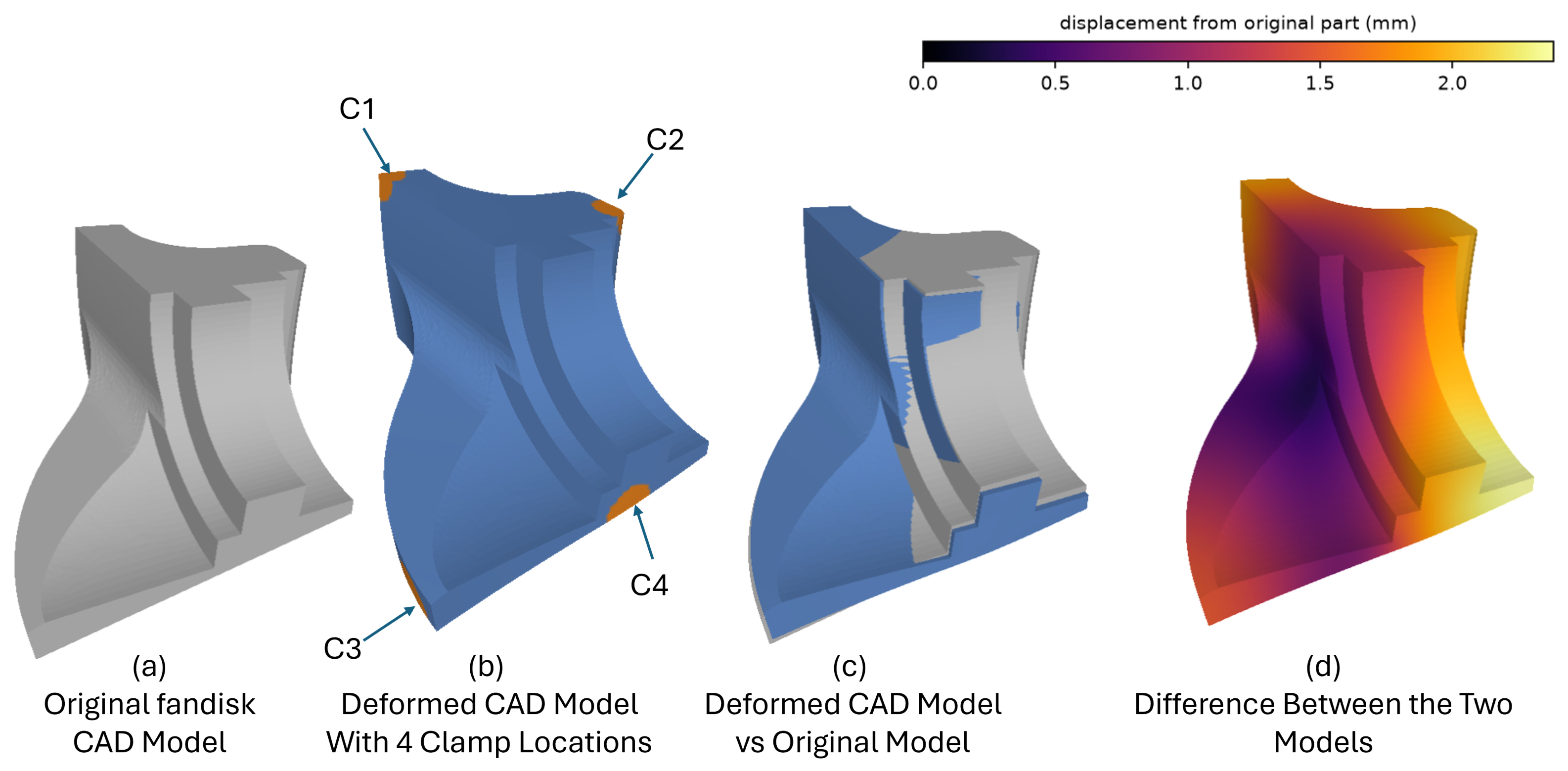
The deformation is applied directly to the full CAD geometry, represented as a STL triangle mesh ( V nom , F ) with n vertices. The mesh is deformed as a whole, rather than through a parametric surrogate such as a fitted NURBS patch or a coarse FEM cage, so the generated free state carries the complete geometric detail of the inspected part. A deformation is encoded as a per-vertex displacement field d R n × 3 , obtained as the minimizer of a discrete surface bending energy defined directly on the triangulation, subject to prescribed displacements at the clamping handles H , the same vertices that the inspection pipeline of Section 3 receives as the clamp indices C ,
min d d L M 1 L d s . t . d H = g .
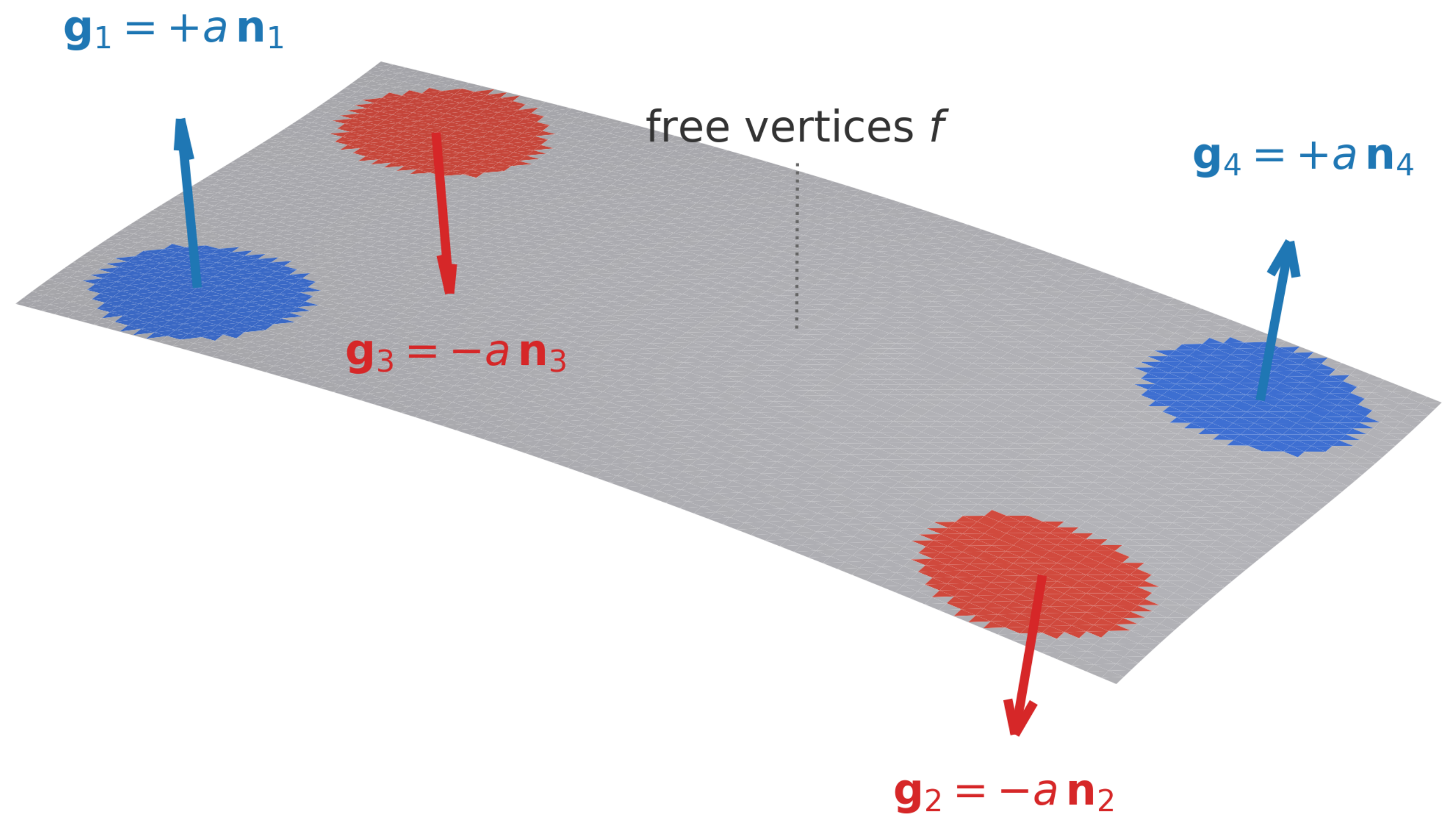
The constraint set mimics the physical fixation of the part: the handles H are small groups of vertices at the locations where the clamps grip the part, and the vector g collects the displacements imposed there, while every other vertex is left free to move as the energy dictates (Figure 7).
In Equation (2), L R n × n is the Laplacian cotangent of the mesh, whose off-diagonal entries L i j = 1 2 ( cot α i j + cot β i j ) sum the cotangents of the two angles opposite the shared edge ( i , j ) , with diagonal L i i = j i L i j ; and M is the diagonal lumped mass matrix, with M i i equal to one third of the total area of the triangles incident to the vertex i. Both operators are assembled directly from the STL faces F , so the energy is intrinsic to the geometry as delivered: no re-meshing, surface fitting, or parametric reconstruction of the part is required at any point. The product B = L M 1 L is the discrete squared (bi-)Laplacian. Its constrained minimizer is the smoothest possible interpolation of the motion of the handle over the entire mesh, the deformation that bends the whole model as gently as the constraints allow. Partitioning the vertices into a free set f and the handle set H reduces Equation (2) to the sparse linear system
B f f d f = B f h g , d H = g ,
So, a single sparse factorization of B f f followed by three back-substitutions, one per coordinate, delivers the displacement field exactly, up to the linear-solver tolerance. Because factorization is reused across right-hand sides, ground truth costs one linear solve per generated free state, which makes it practical to produce large, graded families of test cases spanning many modes and amplitudes.
This deformation generator is the physical foundation on which the entire algorithm evaluation rests, and its choice is deliberate on two counts. First, it produces the right kind of deformation for a thin, compliant part represented by its full triangulation. The squared-Laplacian energy penalizes changes of surface curvature while leaving in-plane extension essentially free, so the free states it generates are smooth and near-isometric: the model bends and twists as a coherent physical shell would, rather than stretching, tearing, or developing localized creases anywhere on the geometry. A deformation drawn from Equation (2) is therefore not an arbitrary warp of the STL but an admissible configuration of it precisely the property the ground truth must have if the recovered deviations are to be meaningful. Second, and central to the fairness of the comparison, the operator B = L M 1 L that generates the data is the same intrinsic operator that regularizes our GB–CICP method in Equation (12). The ground truth thus lives on the manifold of admissible deformations that the intrinsic prior is built to represent, whereas the extrinsic priors of CPD and NICP can only approximate that manifold in the ambient embedding. The benchmark consequently rewards a method not for matching its own generator by construction but for encoding the physically correct notion of bending that all of the compared methods are meant to approximate.
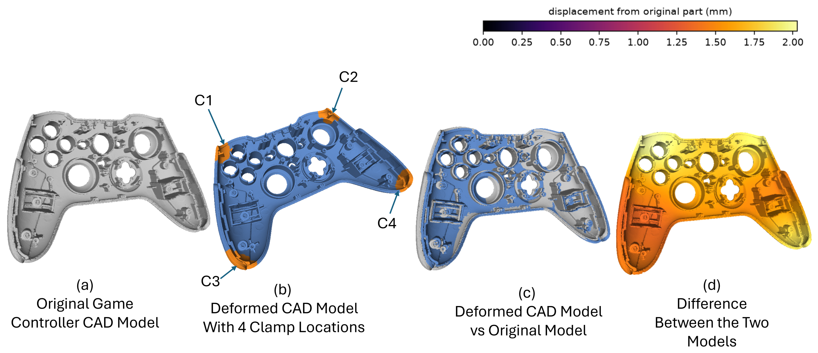
It remains to specify the motion of the handle g . The prescribed displacements are directed along the normal local surface of the STL, which matches the normal bending forces used in the seed study. Writing a for an amplitude scaled to the size of the part, n c for the outward normal at the handle c, and s c { 1 , + 1 } for a sign per-handle, the prescribed motion at the handle c is g c = a s c n c . The sign pattern realizes three canonical modes: a global bend, with all signs equal, bowing the model in phase. A twist, alternating the sign around the boundary so that opposite corners move in opposite directions, and a saddle, assigning the sign by quadrant to produce an anticlastic shape. These are the lowest and softest deformation modes that the constrained mesh admits and hence the configurations that a compliant part most readily assumes in its free state. So, sampling amplitude and sign across them span the dominant flexing behavior of the full model while keeping every generated shape a genuine minimizer of the bending energy. Varying a then controls how far each mode is driven, producing a graded family of free states whose severity is known in advance and whose deformation is admissible by construction. Figure 8 and Figure 9 illustrate the output of the deformation generator on the two parts used for testing. The first, the fandisk, is a prismatic part typical of machined industrial components: its surface is composed of planar and gently curved faces meeting at sharp feature edges, the kind of geometry on which curvature cues are concentrated along a few crisp creases. The second is a video game controller, a considerably more complex but far less feature-rich shape, whose smooth, boxy faces carry much less curvature information than the fandisk’s crisp creases, making both deformation and subsequent registration more challenging. In each figure, the prescribed biharmonic field bends the part between its clamping regions while preserving its local surface detail, producing the physically plausible free-state configurations that serve as ground truth in our evaluation.

5. Pre-Registration Algorithms

This section describes the two rigid registration stages that precede any deformable registration. The first is the pre-registration, which recovers a coarse alignment between the complete CAD model and an arbitrarily placed partial scan. It relies on robust geodesic bilateral curvature descriptors, so that correspondences are driven by intrinsic surface features rather than mere proximity. The second is a robust rigid refinement of this coarse pose, which, since it applies no deformation, doubles as the fixtureless baseline against which the non-rigid methods of Section 6 are measured. Together, the two stages carry the pipeline from an unknown initial placement to a rigidly seated model, leaving as residual exactly the deformation that no rigid motion can absorb.

5.1. Geodesic Bilateral Curvature Registration Algorithm

Every input data point uses nearest-point correspondences, which are meaningful only once the model and the point cloud already share a coarse pose. Failure to do so results in false registrations generated by local minima. Recovering that pose from an arbitrary initial placement is the job of the pre-registration algorithm. This pre-registration is performed using the geodesic bilateral curvature descriptor registration algorithm recently proposed by Boulanger [65]. We summarize the algorithm here and refer the reader to this paper for the full treatment.
The method uses the bilateral filter algorithm, normally a mesh-denoising tool, as a feature descriptor, in four steps:

5.1.1. I-Curvature Field

In a triangle mesh with vertices x i , mixed Voronoi areas A i , and the cotangent Laplacian L , the discrete mean and Gaussian curvatures are
H i = ( L x ) i · n i 2 A i , K i = 1 A i 2 π t i θ i t ,
where ( L x ) i = 2 H i A i n i is the mean-curvature normal and θ i t is the tip angle at i of an incident triangle t. Projecting the mean-curvature normal onto the outward normal n i , rather than taking its length, keeps the sign of H i , which distinguishes a convex from a concave neighborhood and is needed by the shape index below. The principal curvatures follow as κ i 1 , 2 = H i ± max ( 0 , H i 2 K i ) , from which we form the Koenderink shape index and curvedness:
S i = 2 π arctan κ i 1 + κ i 2 κ i 1 κ i 2 , C i = 1 2 ( κ i 1 ) 2 + ( κ i 2 ) 2 .
The pair separates the type of the local shape, carried out by S i [ 1 , 1 ] , from its magnitude, carried out by C i , so that a shallow ridge and a sharp one share a shape index while differing in curvature. Two degeneracies are handled explicitly: the radicand is floored at zero, since H and K are estimated by different discrete formulas and need not satisfy H i 2 K i exactly on a real mesh, and S i is set to zero at umbilic vertices, where κ i 1 = κ i 2 leaves the ratio undefined. Because S i is a ratio of curvatures, it is poorly conditioned when both vanish. The curvature measure C i carries the reliable signal in such near-planar patches, and the bilateral filter of the next step suppresses the residual noise in S i before it reaches the descriptor.

5.1.2. II-Geodesic Bilateral Curvature Filter

Each curvature field f { H , K , S , C } is smoothed by a bilateral filter whose spatial weight is a Gaussian of the geodesic distance g ( i , j ) on the surface and whose range weight is a Gaussian of the curvature difference,
B σ s , σ r [ f ] i = 1 Z i j N i ( σ s ) exp g ( i , j ) 2 2 σ s 2 exp ( f i f j ) 2 2 σ r 2 f j ,
with normalizer Z i the sum of the same weights and geodesic neighborhood N i ( σ s ) = { j : g ( i , j ) 3 σ s } . Geodesic distances come from the heat method or the Dijkstra algorithm. The range term prevents averaging across creases, so ridges survive while within-region noise is removed.

5.1.3. III-Curvature Scale Space and Descriptor

Sweeping the spatial bandwidth on L scales σ s ( ) = ρ h , multiples of the mean edge length h, builds a curvature scale space. Stacking the filtered curvatures across scales gives the per-vertex descriptor
d i = B σ s ( ) , σ r [ f ] i f { H , K , S , C } , = 1 , , L R 4 L ,
which is invariant to rigid motion because curvature is intrinsic, and discriminative because it is multi-scale. The range bandwidth is tied to the estimated scan noise η ^ by σ r = max ( σ r 0 , c η ^ ) , so on noisier data the descriptor widens its range gate and the proportion of correct matches is held up at the source, where it limits the whole pipeline.

5.1.4. IV-Matching and Pose

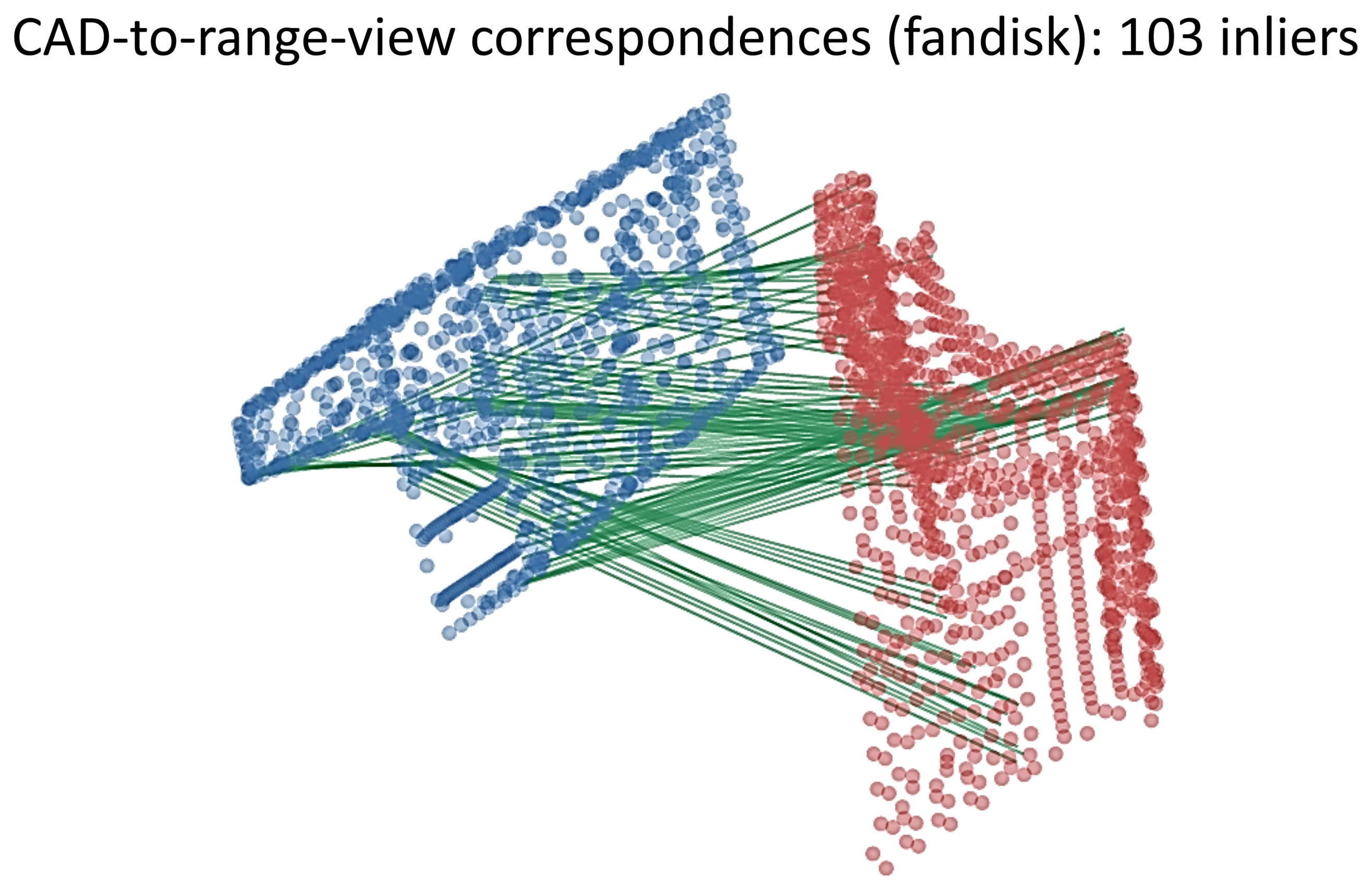
The match is between the complete CAD model and a partial, noisy point cloud, so most model vertices have no scan counterpart, and the two surfaces are sampled and corrupted differently. Two steps make the comparison robust to this. First, the raw descriptors on the two surfaces are brought into a common space by a joint normalization, one shared per-feature mean and variance estimated over both sets, so that the clean, complete model and the partial, noisy scan are compared on equal footing rather than through their separate statistics. Second, the normalized descriptors { d i M } and { d j P } are matched by the mutual nearest neighbors in R 4 L using a Lowe ratio test, so ambiguous matches are discarded. A RANSAC algorithm then draws minimal triplets from the surviving matches, estimates a rigid ( R , t ) by the Kabsch solution of Equation (8), and keeps the transform with the most inliers under an absolute gate R x i M + t x j P τ r , a small fixed fraction of the part diagonal. An absolute rather than residual-relative gate is what lets a correct minority of matches outvote the partial-overlap outliers. Point-to-point ICP from the scan to the transformed model then refines the pose. The Algorithm 1 collects the steps and returns the coarse pose V 0 = R V nom + t .
Algorithm 1 Pre-registration by geodesic bilateral curvature descriptors [65]
Require: complete CAD V nom , partial scan P , scales { ρ } = 1 L , noise estimate η ^ , gate τ r
1: σ r max ( σ r 0 , c η ^ ) ▹ range gate from noise
2:for  Z { V nom , P }  do
3:      compute H , K , S , C on Z ▹ Equations (4) and (5)
4:      for  = 1  to L do
5:             σ s ρ h ; f ˜ ( ) B σ s , σ r [ f ] for f { H , K , S , C } ▹ Equation (6)
6:      end for
7:      assemble raw descriptors d Z ▹ Equation (7)
8:end for
9:jointly normalize { d M } , { d P } to a shared mean and variance
10: M mutual nearest neighbors, Lowe ratio test
11: ( R , t ) RANSAC over M , Kabsch fits, absolute inlier gate τ r ▹ Equation (8)
12:refine ( R , t ) by point-to-point ICP, scan to transformed model
13:return coarse pose V 0 = R V nom + t
This algorithm produces the rigidly posed model that every deformable registration algorithm takes as its starting point. The rigid alignment of Section 5.2 subsequently refines that pose and doubles as the standalone baseline against which the non-rigid methods are measured. What makes the pre-registration a dependable front end is that its matching is feature-aware rather than proximity-driven for the ICP. Correspondence based on nearest points alone breaks down in smooth or flat regions, where many candidate matches lie at nearly identical distances, and the true correspondence is masked by a tangential ambiguity: the surface can slide along itself with almost no change in point-to-point distance, so a purely metric criterion has no way to decide which of the near-tied alignments is the correct one. In practice, this is precisely the failure mode of the ICP that started far from the solution. It locks onto a locally consistent but globally wrong pose. Matching on curvature descriptors dissolves the ambiguity because it anchors the correspondence to an intrinsic property of the surface, one that is carried along with the part under any rigid motion and therefore cannot slide with the pose. Where the geometry is locally uninformative, the descriptor still distinguishes a flat patch near a rounded corner from an identical-looking patch near a crease, and the coarse alignment it returns remains stable exactly where proximity-based matching is weakest.
Beyond this robustness, the pre-registration is deliberately constructed on the same surface representation as our strongest entrant. The geodesic biharmonic curvature ICP introduced below rests on the same intrinsic view of the surface: the geodesic neighborhoods, bilateral filtering, and curvature signatures used here for descriptor matching are assembled from the cotangent Laplacian and the surface metric, the same operators from which the bending prior of Section 6.4 is built, so a single description of the surface serves both the coarse pose search and the non-rigid refinement that follows. This shared foundation amounts to more than an economy of implementation. The features that make the initial alignment reliable are the very features the deformable stage later uses to separate smooth compliant bending from genuine local deviation, so the two stages reason about the surface in consistent terms instead of handing off between mismatched descriptions, each with its own blind spots. Any error mode of the representation is also shared and, therefore, visible, rather than compounded across a change of description. The coarse stage locates the part, and the fine stage deforms it, and because both read the surface through the same intrinsic curvature lens, the transition between them introduces no representational seam. The two stages are not identical in their use of that lens as the descriptor stage filters curvature along geodesic neighborhoods, while the deformable stage penalizes bending through the intrinsic operator alone.

5.2. From Coarse Registration to Rigid Alignment as a Baseline

Rigid alignment serves as both the fixtureless baseline and the initializer for every non-rigid method, so we state it first. Given the putative correspondences between a moving point set A and a fixed set B with weights w i , the rigid weighted fit minimizes i w i R a i + t b i 2 admits the closed-form Kabsch solution
H = i w i ( a i a ¯ ) ( b i b ¯ ) , H = U Σ V , R = V diag ( 1 , 1 , det ( V U ) ) U ,
where a ¯ , b ¯ are the weighted centroids and t = b ¯ R a ¯ . The determinant factor protects against reflections and keeps R S O ( 3 ) . ICP alternates this fit with a nearest-neighbor correspondence step, and for fixtureless data, one detail of that step is decisive: its direction. Since the scan covers only part of the surface, matching every model vertex to the cloud would drag the unscanned regions inward; matching instead each scanpoint to its nearest model vertex ensures that model regions never measured exert no pull. Outliers are suppressed with a Tukey biweight, w i = 1 ( d i / 4.685 σ ^ ) 2 2 for d i < 4.685 σ ^ and zero otherwise, where σ ^ = 1.4826 median i d i is a robust scale estimate. Each iteration costs one k-d tree query per scan point against the n model vertices O ( m log n ) , and the procedure converges within a few tens of iterations. The baseline estimate is V ^ = R V nom + t : no deformation is applied, and the residual is any part of the free-state deformation that a rigid motion cannot absorb.

6. Four Deformable Registration Algorithms

We compare four deformable registration algorithms, ordered by how they constrain the deformation they recover. The RBF–FEM method (Section 6.1) imposes a mechanics-based prior, driving a radial basis deformation from the clamp displacements so that the recovered shape follows the part’s elastic response. Coherent point drift (Section 6.2) treats the scan as samples of a Gaussian mixture and regularizes the displacement field toward global coherence, a purely probabilistic prior with no mechanical content. Optimal-step non-rigid ICP (Section 6.3) attaches an affine transform to every vertex and couples neighbors through a stiffness weight that is relaxed as the iteration proceeds, trading a geometric smoothness prior for freedom as the fit tightens. Finally, our geodesic biharmonic curvature ICP (Section 6.4) penalizes the bending energy of the displacement over the intrinsic surface, enforcing smoothness through the same intrinsic curvature operators used by the pre-registration.

6.1. RBF–FEM: The Original Method

The method of ref. [3] drives a smooth model deformation from the estimated clamp displacements. After rigid pre-alignment to a base V 0 , the position of each clamp c C is compared against the scan: the clamp target t c is taken as the median of the scan points within a small radius of V 0 , c , with a nearest-point fallback when that neighborhood is empty, and the estimated clamp displacement is g ^ c = t c V 0 , c . It plays the role that the prescribed g c of Equation (2) plays in the generator but is recovered from the scan rather than imposed. These sparse displacements are then propagated to the whole model by a multi-quadric radial basis function [66,67]. Placing a center at each clamp and setting a width per-center ε c = min c c V 0 , c V 0 , c equal to the nearest inter-clamp distance, the basis is
ϕ c ( x ) = x V 0 , c 2 + ε c 2 .
The interpolation weights W rbf solve the small dense system Φ CC W rbf = G , where ( Φ CC ) c c = ϕ c ( V 0 , c ) and G stack the clamp displacements, and the deformed model follows as V ^ = V 0 + Φ V C W rbf (Equations (4) and (5) of [3]). The cost is dominated by a | C | × | C | solution and is negligible.
Physical plausibility in this method is not enforced by an explicit mechanical model but is inherited from the structure of the interpolator, which acts as a cheap surrogate for the finite-element elastic response it was designed to approximate. Three properties do the work. First, the multi-quadric kernel is smooth and globally supported, so the recovered field V ^ V 0 varies gently across the surface and contains no local oscillation or discontinuity. The model bends as a continuous sheet rather than deforming point-by-point, which is precisely the behavior of a compliant part that flexes under distributed load. Second, tying the per-center width ε c to the inter-clamp spacing fixes the characteristic length of that bending to the physical scale of the constraints themselves, so the deformation relaxes between clamps over the same distance a real plate would rather than peaking artificially at each fixture point. Third, and most important for inspection, the field interpolates only the handful of clamp displacements and, therefore, lives in a low-dimensional, low-frequency subspace: it can reproduce the smooth, admissible flexure of the part, but is structurally incapable of expressing a small, localized, high-curvature feature. Thus, a genuine defect cannot be absorbed into the deformation and is instead left in the residual, where the deviation report can see it—exactly the separation between admissible deformation and true form error that virtual fixation requires.
However, the same structural property sets the method’s limits. The deformation it can express is exactly as rich as the clamp displacements it can recover: with only a few centers, it interpolates but never extrapolates detail between them, and any elastic behavior finer than the clamp spacing is simply outside its representable space. More critically, its physical fidelity is entirely based on the accuracy of driving displacements g ^ c , and these are estimated at the clamps—precisely the locations where a fixtureless free-state scan is thinnest, since the force-application points are self-occluded and prone to dropout. When data near a clamp are missing, g ^ c is itself corrupted, and because the smooth field faithfully propagates whatever it is given, a corrupted constraint yields a confidently smooth but physically wrong deformation. This is why the method, designed for a fixtured workflow with reliable clamp correspondences, degrades in the fixtureless regime: its mechanism for preserving physical plausibility is sound, but it is anchored to the least observable part of the scan.

6.2. Coherent Point Drift (CPD)

The coherence of point drift [23] casts the registration as the fitting of a Gaussian mixture. The rigidly aligned source vertices Y serve as the mixture centroids, the scan points X are the data, and an expectation–maximization loop alternates between estimating soft correspondences Π i j —the posterior probability that the scan point j was generated by the source vertex i under an isotropic Gaussian of variance σ 2 —and updating a displacement field. The field is regularized by a motion-coherence prior that penalizes non-smooth motion through a Gaussian kernel G i j = exp ( y i y j 2 / 2 β 2 ) , so that nearby points are compelled to move together. The maximization step solves a linear system of the form ( G + λ cpd σ 2 diag ( Π 1 ) 1 ) W cpd = diag ( Π 1 ) 1 Π X Y for the coefficient matrix W cpd , where β sets the spatial scale of coherence and λ cpd its strength. The continuous warp it defines, v v + i exp ( v y i 2 / 2 β 2 ) W cpd , i , is evaluated at every nominal vertex, so the estimate is CPD’s own deformation field rather than an external interpolation. For tractability, the mixture is fitted on a decimated source and target, since the correspondence matrix is dense.
Unlike the RBF method, the CPD enforces physical plausibility through an explicit regularizer rather than through the sparsity of its drivers, and the two parameters β and λ cpd give direct control over the elastic behavior it admits. The motion-coherence prior is a smoothness penalty in a reproducing-kernel Hilbert space: it charges an energy cost to any deformation whose high-frequency content is large, so the field that minimizes it is the smoothest warp consistent with the correspondences, which is the discrete analog of an elastic body preferring the lowest-energy configuration that satisfies its loads. The width β plays the role of a stiffness length scale, setting the distance over which the neighboring material is forced to move coherently: a large β makes the part behave as a rigid sheet that bends only globally, a small β allows more local flexure, and λ cpd trades the overall fidelity to the scan against the adherence to this smoothness. Because the penalty suppresses exactly the high-curvature, short motions that a compliant part cannot physically produce, a genuine localized defect is expensive to reproduce and tends to remain in the residual rather than being fitted away, which is the same admissible deformation versus true form error separation, obtained here from an energy prior rather than from a low-dimensional basis.
The defining feature and the limitation of this prior is that its coherence is measured in Euclidean space: the kernel G i j depends only on the straight-line distance y i y j and is blind to the surface itself. Two points that are close across a fold, a gap, or a thin section are therefore coupled and forced to move together, even though they are far apart along the part and mechanically independent. The regularizer thus encodes a notion of physical plausibility that is correct in the bulk but wrong wherever the part folds back on or near itself. This is precisely the configurations a flexing free-state part is prone to.

6.3. Optimal-Step Non-Rigid ICP (NICP)

The optimal-step formulation of ref. [24] is the closest classical rival to our method and the strongest extrinsic baseline. Each vertex i carries its own 3 × 4 affine transform X i , stacked in a 4 n × 3 unknown X . Writing D for the matrix n × 4 n whose i-th row places the homogeneous vertex [ v i 1 ] in the block of columns belonging to i, the deformed vertices are D X , and the energy is
E ( X ) = W D D X U F 2 + α 2 ( M G ) X F 2 .
The first term drives each transformed vertex to its nearest scan point U i through a robust gate W D . The second is a stiffness term in which M is the node–arc incidence matrix of the mesh edges, so that ( M G ) X measures the difference between the affines of adjacent vertices and G = diag ( 1 , 1 , 1 , γ ) balances their rotational and translational parts. Each step is a normal-equation solve
α 2 ( M G ) ( M G ) + D W D D X = D W D U ,
a sparse system in 4 n unknowns, with the stiffness weight α annealed over a decreasing schedule from a near-rigid start to a flexible fit and the correspondences refreshed at each level.
Where the RBF method preserves plausibility through a sparse basis and CPD through a global smoothness energy, NICP encodes it locally and mechanically: the stiffness term is a discrete elastic energy defined on the mesh connectivity itself. By penalizing the difference between the affine transforms of edge-adjacent vertices, it asks neighboring material to deform consistently, so that the surface bends and twists as a coherent membrane rather than letting individual vertices move independently—a direct discrete analog of an elastic continuum resisting differential strain between adjacent elements. Two design choices give this energy its physical character. The trade-off matrix G = diag ( 1 , 1 , 1 , γ ) separates the rotational from the translational part of each affine, so γ adjusts how much relative sliding is allowed between neighbors before it is penalized as a stretch, and the annealed schedule on α realizes a physically meaningful continuation, beginning almost perfectly rigid and gradually softening the effective stiffness, so the model first captures the global pose and large-scale bending and admits finer flexure only as the stiffness relaxes. This coarse-to-fine relaxation both avoids spurious local minima and, crucially for inspection, prevents a localized defect from being fit early: while the surface is still stiff, the defect is too costly to reproduce and is deferred to the residual, and it is captured only if the final, most flexible level is soft enough to bend into it.
Because the stiffness couples every edge, the prior is richer than the sparse RBF field and, being local, adapts to the mesh rather than to a single global scale. Its limitation is shared with CPD and is the point our method departs from: the prior is extrinsic. It asks neighboring transforms to agree, but measures both neighborhood and agreement in the embedding space rather than along the surface adjacency is the mesh graph embedded in R 3 , and the affine difference is an ambient quantity. The local-affine model also permits stretch and shear, not only bending, so at low stiffness it can express deformations that no inextensible sheet-metal or polymer panel would sustain. The enforced physical plausibility is therefore genuine but ambient: correct where the surface and its embedding agree, yet liable to couple material across a fold or a near self-contact and to admit non-isometric strain, precisely the regimes a surface-intrinsic, near-isometric prior is designed to exclude.

6.4. Geodesic Biharmonic Curvature ICP (GB–CICP)

Our algorithm replaces the extrinsic priors above with the intrinsic thin-plate bending energy that also generates the dataset deformations, and it weights correspondences by surface-orientation compatibility. Working from a rigidly aligned base V 0 , it solves at each iteration for an incremental displacement field e that minimizes the energy
E ( e ) = i = 1 n w i ( V 0 , i + e i ) t i 2 + λ e L M 1 L e ,
where t i is the scan point closest to the current iterate V i and L M 1 L is the same discrete bending operator as in Equation (2). Setting the gradient to zero gives the sparse linear system
W + λ L M 1 L e = W ( T V 0 ) ,
with W = diag ( w i ) and T the matrix stacking the matched scan points t i . The data weight is the product of two factors,
w i = exp d i 2 / 2 ( 3 σ ^ ) 2 Welsch robustness · max 0.05 , | n i · n ˜ j ( i ) | normal compatibility ,
where d i is the distance to the matched scan point, σ ^ the robust scale of Section 5.2, n i the nominal vertex normal, and n ˜ j ( i ) the scan normal estimated locally by principal component analysis. The Welsch factor discounts far matches, while the second factor discounts matches across incompatible surface orientation—precisely where a curved part folds back on itself. The smoothness weight is scaled to the operator magnitude, λ = λ 0 / diag ( L M 1 L ) ¯ , so a single λ 0 is transferred across meshes of different resolution, and it is annealed by a factor of 0.8 per iteration, so the fit starts smooth and relaxes toward the data.
In this method, the physical plausibility of the recovered surface is preserved by construction rather than approximated. The regularizer e ( L M 1 L ) e is a discrete thin-plate bending energy: it charges a cost proportional to the change in curvature that the displacement induces, so the minimizer is the configuration that reaches the scan while bending as little as an elastic plate would. This is the same energy that generates the synthetic free states, so the prior encodes exactly the class of deformations the parts actually undergo. The model is regularized toward the true manifold of admissible flexure rather than toward a generic notion of smoothness. Three properties make this constraint faithful. First, the operator is intrinsic: because L M 1 L is built from the surface metric, smoothness is enforced along the part and never across the gaps between folds that mislead a Euclidean prior, so material that is far apart geodesically is left mechanically independent even when it is near in the embedding. Second, the bending energy penalizes only change of curvature, not membrane strain, matching the near-inextensible behavior of sheet-metal and polymer panels that bend freely but resist stretching. The warp it favors is therefore close to isometric, as a real compliant part’s free-state flexure is. Third, annealing on λ realizes a stiff-to-flexible continuation analogous to gradually releasing a physical constraint: the surface first accepts only global low-curvature bending and is allowed finer flexure only as the penalty relaxes, so a localized defect, being high-curvature and geodesically compact that remains too costly to absorb and is left in the residual for the deviation report to see, rather than smoothed into the deformation.
Two further choices keep this physical prior clean. The curvature-compatibility factor in Equation (14) refuses correspondences whose surface orientation disagrees, so the bending energy is never driven by matches that would fold the model against its own normals. The data term is made consistent with the same intrinsic geometry that the regularizer assumes. And the increment is measured from the aligned base V 0 rather than from the raw nominal, which keeps the rigid pose out of the bending penalty, were it measured from the unaligned model, the operator would spuriously penalize the very rotation needed to seat the model on the scan and so misattribute pose to elastic energy. The net effect is a registration whose deformation is physically admissible by the same standard used to create the ground truth, at negligible cost: each outer iteration is a sparse Cholesky factorization of a n × n matrix with three right-hand sides, comparable to a single linear solution, so the method runs in a couple of seconds per part.
Algorithm 2 Geodesic biharmonic curvature ICP (GB–CICP)
1: V 0 robust partial-overlap rigid ICP of V nom to P Section 5.2
2: Q L M 1 L ;    λ λ 0 / diag ( Q ) ¯ ;    V V 0
3:precompute nominal normals n and PCA scan normals n ˜
4:for  iter = 1  to T do
5:        t i , d i nearest scan point to V i for all ik-d tree
6:        w i Welsch ( d i ) · normal-compatibility ( n i , n ˜ j ( i ) ) ▹ Equation (14)
7:       solve ( W + λ Q ) e = W ( T V 0 ) ▹ Equation (13), 3 RHS
8:        V V 0 + e ;    λ 0.8 λ
9:end for
10:return  V ^ = V

6.5. Shared Settings and Complexity

All four non-rigid methods receive the same rigid initialization and the same clamp indices, and all return an estimate on the nominal vertex set, so that the metrics of Section 7.2 apply uniformly and any difference in the reported accuracy can be attributed to the deformation prior alone rather than to differences in setup or output representation. Automatic discovery of the clamping vertices lies outside the scope of the present study and is left as an evaluation stage for future work. Here, the indices are supplied, so that the comparison isolates the registration itself and is not confounded by errors in locating the constraints.
Beyond accuracy, the methods occupy different points on a cost-versus-prior trade-off, and the ranking by expressiveness of the deformation prior is largely mirrored by the ranking in computational cost. At one extreme, the rigid alignment and RBF–FEM are effectively free: the former solves a small pose problem, and the latter a dense system only as large as the handful of clamps, so both complete in negligible time, but their deformation models are correspondingly limited. GB–CICP sits next, costing one sparse Cholesky factorization of an n × n matrix per outer iteration and completing in about two and a half seconds per part, which buys the full intrinsic bending prior at a cost comparable to a single linear solve. CPD is appreciably more expensive, dominated by the dense correspondence matrix formed in the expectation step of its mixture fit, which remains costly even with the source and target decimated for tractability. Optimal-step NICP is the most expensive of the four, solving a larger 4 n system—four unknowns per vertex—at each of several annealed stiffness levels, and runs some five to six times slower than GB–CICP. These timing figures are reported in Table 5 of Section 8.5, so that the precision of each method can be read against the computational price it demands—a trade-off that matters directly when the process is to be moved from the metrology room to the production line.

7. Testing Methodology

The objective of this section is to define the structure of a dataset sample, to explain how each sample is generated deterministically from a single random seed, and to show why this construction yields a reproducible benchmark with exact ground truth, something no physical acquisition campaign can provide.
A data set sample is a triple consisting of a nominal CAD surface, a deformed version of that surface, and a scan of the deformed surface acquired with the virtual scanner of Section 4.2. The nominal surface is the STL mesh designed. The deformed surface is the free state configuration produced by the bending-energy generator of Section 4.3, and the scan is the partial noisy point cloud returned by the virtual scanner from that free state. Located alongside the triple is the displacement field that carries the nominal mesh onto the deformed one, which serves as the ground truth. Because this field is expressed on the nominal vertex set, it provides the exact free-state position of every point, a reference against which any recovered surface can be scored and one that no physical acquisition could supply.

7.1. Scanning Two Deformable CAD Models

Given an STL file generated by a CAD system, the toolkit selects clamping handles automatically from the part’s principal extent, assigns an inspection tolerance, and runs the same inspection pipeline for each algorithm. We demonstrate this on the two generated test parts, the fandisk and the game controller housing. The physically scanned part of Section 8.4 is acquired with a real sensor and is not subject to this model. The two parts are also acquired with different numbers of viewpoints, chosen to match how much of each surface a real scanner could reach: the fandisk is scanned from two views and the more strongly self-occluding controller with four viewpoints.
Figure 5 illustrates the scan generator on the fandisk model, shown below, the side that houses the characteristic grooves, so that the deformation and deviation patterns on the inspected face are legible. The shaded mesh is the CAD reference (a); a virtual scan from two viewpoints, with the acquisition cameras and their view frustum drawn in, returns the partial point cloud a real scanner would see (b); and a prescribed deformation is applied to the part and recorded as exact ground truth (c). Two views suffice here, because the fandisk is largely convex and its flat faces present favorable incidence over a wide angular range, so a pair of opposing poses already covers the inspected face with little grazing loss. The prescribed deformation is a moderate-amplitude bend combined with a mild twist, with the handle motion set to a = 2% of the diagonal of the bounding-box (about 2 mm on this part). The resulting displacement field has an RMS of 1.40 mm, and a rigid comparison alone leaves a normal-deviation RMS of 1.41 mm (Table 5), against the ±2.25 mm tolerance that the rule of Section 7.2 gives for this part. The amplitude is chosen so that the crease-rounding failure mode is visible: a smoothing prior tends to round exactly the sharp edges that define the part, and at this amplitude, that error is large enough to carry a method past the pass threshold.
Figure 10 is the same for the game controller housing, a case with the opposite character: no sharp features, but a large, boxy body whose smooth, weakly curved faces carry little curvature information. The face is shown from the top shell that the automatic orientation stage selects for scanning. The same three panels are shown. Shaded CAD reference (a), a virtual scan of four viewpoints with cameras and view frusta (b), and a prescribed free-state deformation kept as exact ground truth (c). Four views are used here rather than two because the controller’s grips and deeply recessed underside are self-occluded from any single direction. Two views would leave large no-data regions across the curved flanks, whereas four poses distributed around the shell recover a connected outward-facing surface while still leaving the underside and grip interiors as genuine gaps. The deformation is a smoother and more globally distributed flexure than the fandisk’s with a global bend combined of a mild twist, giving a displacement field of 1.44 mm RMS that reaches roughly 2 mm at the upper edge and the grip tips. The amplitude reflects the greater extent of the part rather than any greater physical compliance: as noted in Section 8.2 the thin-plate generator is exercised here in a solid housing and is not a mechanical model of it. Where the fandisk tests whether a method preserves creases, the controller tests whether it recovers this large smooth flexure from a scan that covers only the outward-facing shell, exercising the missing-data regime the earlier sections emphasized.
For each part, the recovered deviation, scored only on the vertices the scanner actually measured, so that occluded interiors and clamp regions appear as gaps rather than spurious deviation, is reported with the results in Figure 6. This is the same workflow as the evaluation scores, applied to models that did not come from the procedural set, and is how a user would point the generator at their own parts. Concretely, the loader cleans the mesh, optionally rescales it to a target size, and densifies or decimates it. It then selects the handles as the vertices nearest the corners of the part’s principal (PCA) bounding rectangle, so the choice is orientation-independent, and, when no thickness is supplied, sets the tolerance to a small fraction of the bounding-box diagonal. Scoring is finally restricted to the vertices the scanner actually measured, which excludes occluded interiors and the far side of a closed solid, so the reported deviation reflects only what the inspection could have observed.

7.2. Evaluation Protocol

A registration algorithm uses only the nominal CAD model, the scan point cloud, and the clamping vertex indices, and returns an estimated deformed surface V ^ on the nominal vertex set. It never sees the ground-truth displacement field or the point-to-vertex correspondence recorded by the generator. This separation is what makes the score meaningful: the algorithm is given exactly the information available on a real shop floor and is graded against information that only the synthetic construction possesses, so nothing about the answer can leak into the method that produced it.
Because the scanned data lie on the surface of the CAD model rather than on a set of tracked material points, we score inspection deviation rather than raw displacement. With n i being the unit outward normal of the true deformed CAD surface, let e i = | ( V ^ i V i true ) · n i | be the deviation per-vertex along that normal (Figure 11). This is deliberately the quantity on which a deviation report acts: the residual between the estimate and the truth splits into a normal component, which lifts the surface off where it should sit and is genuinely observable, and a tangential component, which merely slides the estimate along the surface without changing the geometry. Tangential sliding is not a defect and, because it moves a point to another location on the same surface, cannot even be recovered from surface samples. So, counting it would penalize a method for an ambiguity inherent to surface measurement rather than for any real error. Scoring only the normal component thus aligns the metric with what physical inspection of the part could actually detect.
Two distinct residuals appear in what follows and should not be conflated. The inspection deviation e i defined here compares the estimate with the ground truth. It is available only in generated data, where it is the quantity reported in Table 1 and Table 2 and is displayed in the deviation maps. The scan-to-model residual used in Section 8.1 to trace convergence instead compares the registered surface with the measured points. It is the quantity a real deployment can compute, and being a fit residual against noisy, one-sided data rather than an error against the truth, it is bounded below by the scan noise. For a method that fits the scan closely, the fit residual is the larger of the two—GB–CICP recovers the surface to 0.12 mm of inspection deviation while sitting at a 0.28 mm scan-to-model residual, while a method that misfits badly shows the reverse, since a deformation driven to the wrong shape departs from the truth faster than it departs from the sparse points it was fitted to. The two numbers are therefore not comparable across methods and are never mixed below.
Across the set of scored vertices S , we summarize the deviation with three complementary statistics: the root-mean-square value RMS = 1 | S | i S e i 2 , which reflects the typical accuracy across the entire surface. The maximum max i S e i , which captures the single worst point, and the 95th percentile P 95 , a robust stand-in for the worst case that a single outlier or a noisy normal estimate would otherwise distort. Reporting all three matters because they can disagree: a method may achieve a low RMS by fitting the surface well on average but incur a large maximum precisely at a crease, a feature edge, or a localized defect, and it is that tail, not the mean, that governs whether a real part is correctly judged.
Acceptance follows the seed study, with the tolerance adapted to a general CAD model rather than to a thin plate of a single known thickness. The geometric tolerance τ is taken as half the local wall thickness when the CAD model provides one. For an arbitrary STL solid, where no single thickness is defined, τ is set instead to a small fixed fraction of the part’s bounding-box diagonal, so that the criterion scales with the size of the part and remains well-defined on any geometry. The fraction is stated with each part. The fandisk’s ±2.25 mm occupy about 2.25% of its bounding-box diagonal. Two further conditions, introduced in Section 10 and motivated there, apply to every result in this paper: τ must exceed the measured chain floor of Section 9, so that the tolerance is one that the measurement system can resolve, and acceptance requires both an area criterion and a region criterion, because the area criterion alone admits localized defects. A vertex is in tolerance if e i τ . A part passes the area criterion if at least 95% of its scored area is in tolerance, so that a few borderline points do not reject an otherwise conforming part and overall pass only if it also satisfies the region criterion. The set of scores S depends on what the inspection could observe: for procedural parts whose full surface is generated and visible, every vertex is scored, while for a closed or partially visible CAD solid, the set is restricted to the vertices the scanner actually measured, since a deviation cannot be claimed where nothing was observed. This keeps the pass/fail decision honest—occluded interiors and the far side of a closed body appear as gaps rather than as spurious deviation or unearned agreement.

8. Results

8.1. The Fandisk: Pre-Registration and Deformable-Stage Accuracy

As mentioned previously, the part CAD model is first automatically oriented by using a principal-component analysis of the mesh to identify its dominant face, and then the requested side is turned toward the scan simulator. This allows the CAD file saved in an arbitrary orientation to be aligned with the virtual scanner. The oriented part is then placed in a known pose such as a rotation of 121.4°, specified by the extrinsic Euler angles (120°, 45°, 10°), combined with a translation. The scan simulator next performs a virtual scan from two orthographic views, which are automatically selected by aiming each view against the mean surface normal of the posed part so that the visible faces are well covered. A Gaussian range noise of zero mean and 0.02 mm standard deviation is added to the points synthesized along the viewing direction to simulate acquisition noise. The result is a single partial point cloud, which combines both views, which covers 51% of the surface of the part (Figure 12, red).
This partial scan is registered on the complete CAD model (blue) with the geodesic bilateral curvature descriptor algorithm of Section 5.1. Each surface point carries a 16-dimensional descriptor: four geodesic scales { 1.5 , 2.4 , 3.8 , 6.0 } h , in units of the mean length of the edge, each contributing to the mean curvature H, the Gaussian curvature K, and the shape and curvedness indices S and C. The model and scan descriptors are jointly normalized to a shared mean and variance, so the complete, clean model and the partial, noisy scan are compared on equal footing, and candidate correspondences are determined by mutual nearest neighbors in this descriptor space. As mentioned in Section 5.1, the RANSAC search algorithm then draws minimal subsets from these candidates, keeping the rigid transform with the most inliers under an absolute distance gate. The final pose is then computed from the inliers using a point-to-point ICP algorithm. The partial overlap and the scan noise make this substantially harder than aligning two complete meshes because most model vertices have no counterpart in the scan, and the two surfaces are sampled and corrupted differently. nevertheless, matching succeeds independently of the initial pose between the CAD model and the scanned data: for the fandisk, 209 mutual matches are initially found, of which a geometrically consistent subset of 103 survives as RANSAC inliers.
Figure 13 trace the residual RMS from scan-to-model through the entire pipeline, now measured against a deformed scan of the fandisk. This is the fit residual of Section 7.2, not the inspection deviation of Table 2. The two are reported on different scales for the reasons given there. The RANSAC initialization delivers a coarse pose with a residual of 0.87 mm, and the rigid ICP refinement settles within the first iterations onto a plateau of 0.86 mm so that no further rigid iteration is necessary. This plateau is not a failure of the pose search: with the part physically deformed (the imposed deformation field has an RMS of 1.40 mm), 0.86 mm is the floor attainable by any rigid transform, and the flat curve shows that the pre-registration has already extracted all six rigid degrees of freedom after RANSAC. Recovering the remaining residual is precisely the task of the deformable stage. Starting from this rigid estimate, the proposed GB–CICP drives the residual to 0.28 mm within about five iterations, matching the non-rigid ICP baseline (0.26 mm) while remaining well below the methods that fail to model the deformation adequately: coherent point drift stalls at 0.65 mm, and the RBF–FEM variant overshoots to 1.45 mm, worse than the rigid plateau itself. The recovered pose and subsequent deformable correction are therefore accurate to well within the inspection tolerance. In the evaluation this coarse pose is available by construction, since the nominal mesh and the scan share a coordinate frame, so the deformation results reported below isolate the deformation prior rather than the pose search. The pre-registration is exercised here to show that the pipeline recovers an adequate starting pose even when the scan is delivered in an arbitrary placement. Figure 14 shows the CAD model and the range view before alignment and, once the recovered pose is applied, the scanned region of the CAD model shaded by its residual difference from the registered scan.
Table 2 compares the four deformable registration algorithms. All deviations are measured along the surface normal, the quantity a deviation report uses. GB–CICP posts the best value in every column: an RMS of 0.12 mm, a 95th-percentile deviation of 0.05 mm that is more than forty times within the tolerance of ±2.25 mm, and the tightest worst case at 1.40 mm. NICP is a close second on the bulk statistics (0.14 mm RMS, 0.07 mm P 95 ) but leaves a larger localized excursion of 1.75 mm, and for an acceptance rule, it is the worst-case excursion, not the average, that decides whether a part passes the inspection process. CPD trails at 0.47 mm RMS: on this partial scan its Euclidean coherence prior fails to engage the twist, leaving a residual three to four times above the two locally coupled priors. RBF–FEM, starved by deliberately missing data in the clamps, fails outright at 2.56 mm RMS with a maximum of 7.19 mm, well outside of tolerance. The ordering is monotone in how well each method’s non-rigid freedom is matched to the data: freedom anchored to missing data (RBF–FEM), a loosely coupled prior that cannot engage the twist (CPD), and the two locally coupled priors (NICP, GB–CICP) that resolve it.
The choice of metric does the real work here. In this part, roughly half of the applied twist is tangential sliding: motion that carries surface points along the surface without moving the surface itself and that no range scan can observe, since a scanner sees where the surface is and not how material slid within it. A point-to-point error would therefore be dominated by this unobservable, and in fact irrecoverable, tangential component, which is neither a defect nor something any method could or should undo. Under such a score, every algorithm appears to collapse onto a common floor, and the comparison loses its power to discriminate. Measured along the surface normal, however, the tangential motion drops out by construction and the algorithms separate cleanly. What remains after the normal projection is exactly the quantity that a dimensional deviation report would flag, so the metric that makes the methods distinguishable is also the metric that matters for inspection.
The direct comparison of GB–CICP with NICP and CPD is the reason that those two are included alongside our method. GB–CICP and NICP share a structural feature: both priors couple the deformation of neighboring vertices, so a displacement imposed in one region is propagated smoothly to its surroundings. That coupling is what allows them to engage the global twist and drive the bulk of the residual down to a small multiple of the scan noise. CPD’s prior, by contrast, enforces coherence through a Gaussian kernel in the ambient Euclidean space rather than along the surface, and on this partial scan that coherence is too weak to recover the twist. The missing and one-sided data leave its Euclidean field under-constrained, which is precisely the partial-overlap regime that later Bayesian formulations of coherent point drift were introduced to address. Between the two front runners, GB–CICP leads on all three error statistics and most meaningfully on the worst case, 1.40 against 1.75 mm, where NICP’s remaining error concentrates in a single localized excursion rather than spreading thinly across the surface. A concentrated worst case error is the more dangerous one for inspection, because it is what a tolerance test is meant to catch.
One caveat must be clarified. GB–CICP’s smoothness term is the same discrete biharmonic operator that generates the prescribed deformation, so on this dataset it carries an inductive-bias advantage: the ground truth lives on exactly the manifold of shapes its prior favors. Real scans, whose true deformation is set by the part’s physics and matches no prior model by construction, would remove that advantage. The fair competitive reading is therefore the conservative one: GB–CICP and NICP are the two front runners, with GB–CICP ahead on this part, and the decisive test that separates them is one run on data drawn from no method’s prior. Section 8.4 provides that test. The physical part measured there is deformed by gravity and free-state handling rather than by any operator we chose, so no method’s smoothness prior is privileged, and the synthetic margins reported in this section should be read as favoring GB–CICP by construction until they are confirmed there. We state this in the strongest form available to us: the numbers in Table 1 and Table 2 are not evidence that GB–CICP’s prior is correct, only that it matches the generator. The evidence that continues the question is given in Section 8.4.
The RBF–FEM outcome deserves a fair reading of its own, because taken out of context, its large error could be mistaken for a failure of the method rather than of its operating assumptions. RBF–FEM was designed for a fixtured workflow in which the clamp correspondences are reliable and densely informative, and in that setting it delivered the order-of-magnitude speed-up that motivated it. The present evaluation deliberately places it in the harder fixtureless regime, with data missing precisely at the clamp locations, no-return regions, and the seed study itself identified around the force-application points. In that regime its few-center radial-basis extrapolation is starved of exactly the clamp information on which it depends, and the deformation it reconstructs away from the centers is correspondingly unconstrained. The evaluation therefore does not contradict the original result: it locates the boundary of the method’s operating envelope, showing where a fixtured-workflow prior ceases to hold once the fixture and the data it would have provided is removed. Mapping that boundary is one of the things that a controlled comparison of this kind is for.

8.2. A Second CAD Model: The Game Controller

To show that the preceding results are not tuned to a single part, we repeat the fandisk experiment end to end on a second, more complex CAD model: a game controller housing, taken exactly as it arrives from the CAD system, with no cleanup, remeshing, or manual preparation. Its tessellation contains 299,693 triangles, which the program first decimates into 153,240 faces. The part is then automatically oriented, and the algorithm selects the top face to scan. The posed part is scanned from four automatically selected views with the acquisition noise set at 0.02 mm, producing a partial cloud that covers 48% of the surface. Every stage that follows runs with the same settings as the fandisk run, and nothing is retuned for the new geometry.
The controller is a deliberately adversarial case for the descriptor. Its largely smooth, boxy faces carry far less curvature information than the fandisk’s feature-rich surface, so the descriptor space is crowded with near-duplicates: of 606 mutual descriptor matches, only a geometrically consistent subset of 10 survives as RANSAC inliers. That sparse subset is nevertheless sufficient for RANSAC to produce a pose close enough for ICP to converge. The coarse pose is rough with a scan-to-model residual of 7.9 mm RMS, an order of magnitude above the fandisk’s 0.87 mm starting point. This is why the rigid ICP works correspondingly harder, decaying over some 25 iterations rather than settling within the first few (Figure 15). It converges all the same to a plateau of about 1.4 mm. This plateau is not a failure of refinement: the scanned part carries a deformation field of 1.44 mm RMS, so 1.4 mm is the floor attainable by any rigid transform, and the flat tail of the curve shows that the six rigid degrees of freedom have been fully extracted. Figure 16 shows the model and the view of the range before and after this alignment. As in the fandisk, recovering the residual that remains below this floor is precisely the task of the deformable stage.
Table 1 scores the four entrants in deformable-stages on the controller along the surface normal, the amount a deviation report uses, and the order reproduces the fandisk ranking. GB–CICP again posts the best value in every column: 0.12 mm RMS, a 95th percentile of 0.17 mm, and the tightest worst case at 1.55 mm. NICP is again a close second in bulk statistics (0.14 mm RMS) and essentially ties the GB–CICP’s maximum (1.56 mm), though its wider 95th percentile (0.25 mm) shows the residual spreading over more of the surface rather than concentrating in a single excursion. CPD trails at 0.76 mm RMS, further behind than on the fandisk, consistent with its loosely coupled Euclidean prior degradation as the scan becomes sparser and the geometry less prominent. RBF–FEM, starved once more of the clamp data on which its few-center extrapolation depends, fails outright at 2.67 mm RMS with a maximum of 7.31 mm. The repetition is the point: the same ranking, with nearly the same front-runner margins, emerges on a part with different topology, different curvature content, and different coverage, which says the pipeline’s behavior transfers across geometries rather than being fitted to one.
The conformance reports behave as they did on the fandisk. The free-state part passes cleanly, with 100% of the scored points in tolerance at a scan-to-model RMS of 0.16 mm, while the same part carrying the prescribed boss defect fails, with only 90.0% of the scored points in tolerance. The report therefore does in this geometry what an inspection report must do: separate a compliant part from a defective one, with the defect localized rather than smeared into a global misfit. One qualification applies, and we state it plainly. Unlike the thin-shell parts of the dataset, the controller is a solid housing, so the thin-plate deformation model is not a physical model of its compliance. In reality, a solid part of this stiffness would not deform by millimeters in the free state. The run should accordingly be read as exercising the pipeline stages—pre-registration, registration, and reporting—on a challenging geometry, not as a mechanical simulation of this particular part.

8.3. Defect Detectability Against Size and Magnitude

A non-rigid registration that is free to deform the nominal onto the measurement can absorb a localized defect into the deformation field, in which case the defect disappears from the residual and the part passes. This is the central failure mode of the entire approach and the guards described in Section 6.4 exist to prevent it. This section measures how well they do so, because a qualitative argument is not sufficient for a criterion on which a conformance decision rests.

8.3.1. Simulation Test Geometry

To study detectability, we use a third synthetic geometry, distinct from the two parts of Section 8.1 and Section 8.2, and we describe it here because the choice is dictated by the study rather than by preference.
The part is a doubly curved open shell, shown in Figure 17. Writing u 1 , u 2 for the two principal directions of the vertex distribution and u 3 for its normal, the surface is a graph over its own mid-plane,
S = c + ξ 1 u 1 + ξ 2 u 2 + w ( ξ 1 , ξ 2 ) u 3 : ( ξ 1 , ξ 2 ) Ω ,
with c the centroid, Ω R 2 the trimmed in-plane domain, and w a smooth single value height. Its bounding box is 174 × 110 × 42 mm, giving a bounding diagonal of d = 210.0 mm. The extent of the in-plane is roughly 95 × 66 mm and the out-of-plane range of w is 38.1 mm, so the shell rises by about a fifth of its width. The surface carries 19,144 mm2 area on 8544 vertices and 16,650 triangles, is open with 436 boundary edges and is single-sided: it has no back face, so all it is reachable with a modest view set.
In what follows, two differential properties matter. The median absolute mean curvature is | H | = 5.2 × 10⁻³ mm−1, a radius of curvature of about 192 mm, so the shell is gently curved relative to its size and the defect amplitudes that the grid below varies over, 0.30 to 1.50 mm, are small perturbations of it. The median absolute Gaussian curvature is | K | = 2.6 × 10⁻⁵ mm−2, about two orders of magnitude below H 2 , so the surface is free from the sharp creases on which the curvature descriptors are concentrated. It is therefore a hard case for pre-registration and an easy one for the deviation measure, which is the combination a detectability study wants: the defect must be resolved against a smooth background rather than against surface detail.
The median edge length is 1.894 mm, or 0.90% of the bounding diagonal. The grid below varies the width of the defect σ from 3 to 12 mm, so the narrowest defect spans approximately three elements and the widest about thirteen. This is the property that decides the choice of host. A detectability grid requires defects several times wider than the tessellation, so that a recovered amplitude reflects the surface and not the mesh, and it requires the defect region to be densely covered. The fandisk does not satisfy either: its median edge is 1.3% of its diagonal, so the narrowest defect here would barely cover one element, and being a closed solid, its coverage from the same view set falls below a third. Running the grid on it returns recovered amplitudes exceeding the true ones by an order of magnitude, which measures the part’s own registration residual rather than any defect.
That requirement is itself a limit on the method, and we state it as one. On a part whose mesh is coarse relative to the defects sought, or whose coverage is low, the deviation field cannot resolve defects at all and no parameter setting repairs it. The fandisk is such a part under the view set used here, and Section 8.4.4 shows that the physically scanned engine cover is another, for different reasons and by a much wider margin.

8.3.2. Definition of Detectability

A defect is detectable when the deviation it produces is large enough to be distinguished from the deviation that the pipeline reports everywhere else. Both terms are needed: an amplitude alone says nothing without the level from which it must be separated, which is why we report a ratio rather than a recovered depth.
Let the prescribed defect be a Gaussian bump of amplitude a and characteristic width σ , applied along the normal surface and centered at x 0 in the free-state configuration of the shell of Section 8.3.1, so that the displacement at a point x is
δ ( x ) = a exp x x 0 2 σ 2 n ( x ) .
Let e i be the inspection deviation of Section 7.2 at the scored vertex i, let C be the set of vertices that survive the coverage mask and the boundary exclusion, and let r i = v i x 0 be the distance from vertex i to the defect center. Partition of the scored vertices into a defect neighborhood and a background,
D = { i C : r i R d } , B = { i C : r i > R b } ,
with fixed lengths R d and R b fixed lengths, held constant throughout every cell of the study, chosen so that R d exceeds the widest defect considered and R b is comfortably beyond its skirt, here R d = 12 mm and R b = 60 mm. With the width convention of (16) the narrowest bump has fallen to 1.1 × 10⁻⁷ of its peak at R d and the widest to 0.37, while every width is below 10−11 at R b , so D contains the peak and the informative skirt of the defect at every width while B is free of it well below the noise floor.
The recovered amplitude is the largest deviation reported inside the defect neighborhood, and the background is a high quantile of the deviation reported far from it.
a ^ = max i D | e i | , b = Q 0.95 { | e i | : i B } ,
with Q 0.95 the 95th percentile. The detectability is their ratio,
ρ = a ^ b = max i D | e i | Q 0.95 { | e i | : i B }
and the recovery fraction is a ^ / a , reported as a percentage. The localization error is r i with i = arg max i D | e i | , the distance from the recovered peak to the true center.
Three choices in (18) and (19) are deliberate. The numerator is a maximum rather than a mean because a defect is a local extremum, and an inspector acts at its peak. The denominator is the 95th percentile rather than the maximum, because the background maximum is itself an extreme value over many vertices and is dominated by the boundary of the measured region, which would make ρ a statement about the mask rather than about the defect. And both are taken in | e i | rather than in the signed deviation, because a defect may be proud or sink while the background is two-sided.
Fixing these radii rather than scaling them with σ is essential, and we record why because the natural choice is the wrong one. If D is taken as r i 3 σ , its area grows as σ 2 , so a wide defect takes its maximum over an order of magnitude more vertices than a narrow one, and since a ^ in (18) is a maximum, its expectation grows with the sample count even when no defect is present. If B is taken as r i > 5 σ it simultaneously retreats to a different and quieter part of the surface. Both effects flatter the widest cells. Under σ -scaled windows, the smallest amplitude in this study returned ρ = 2.1 at σ = 7 mm but ρ = 3.6 at σ = 12 mm, apparently improving as the defect widened, which is physically impossible for a smoothness-regularized fit. Inspecting that cell shows a reported peak of 0.150 mm taken over 1085 vertices against a true recovered peak of 0.044 mm near the center, so the figure was the largest of a thousand background samples rather than the defect. With fixed radii, the same row reads 3.7, 1.5, 1.1, monotone in σ as it must be. Any study of this kind should hold the windows fixed, or report a ^ at the known center rather than as a windowed maximum.
We call a defect reliably separable when ρ 3 . The threshold is a convention, not a derivation: with the background defined at the 95th percentile, ρ 3 places the recovered peak far enough above the bulk of the deviation field that a region-based acceptance criterion (Section 10) will isolate it rather than merge it into the surrounding form error. Values near unity mean that the defect is indistinguishable from the background and the pipeline has not detected it at all, whatever amplitude it reports.
Note that ρ is a property of the measurement chain and not of the part alone. It depends on acquisition noise, coverage, registration, and in particular on the band-limit , which is the subject of the results below.
Table 3 crosses the defect amplitude from 0.30 to 1.50 mm, against the spatial extent of the defect, σ { 3 , 7 , 12 } mm, in fixed acquisition noise of 0.03 mm, with every other parameter at the values used throughout Section 8. Each cell reports a ^ / a , b and ρ as defined above. The localization error, discussed below, is 0.4–2.1 mm in every cell with ρ > 1 and is omitted from the table for space. Figure 18 shows the twelve prescribed defects in the host geometry, so that the amplitude a and width σ that are being varied can be seen directly rather than inferred from the table.

8.3.3. Simulation Results

The deformation in every cell is drawn from a closed-form analytic field, an explicit function of the part’s two in-plane principal coordinates applied along the surface normal, which is the minimizer of no bending energy and therefore shares its prior with no entrant. This is how we discharge, for this experiment, the concern raised in Section 4.3. The grid is repeated with the biharmonic generator of that section, and a comparison is reported among the conclusions in the following.
Figure 19 follows one cell of the grid, a = 0.90 mm at σ = 7 mm, throughout the pipeline in this geometry, so that the numbers in Table 3 can be read against the fields that they summarize. The prescribed free-state deformation reaches 4.53 mm, about 2 percent of the bounding diagonal and five times the defect it conceals. The fit recovers 3.69 mm of it, and the deviation the inspection reports drop from 0.585 mm RMS under a rigid best fit to 0.062 mm after virtual fixation, a factor of nine. The defect itself, invisible on the rigid map because compliance dominates it everywhere, emerges at +0.826 mm against a true +0.90 mm once the compliance is removed.
Five conclusions follow, and three of them qualify the claims made earlier in this paper.
The single-pass band-limit trades recovery against background, and the default sits at the wrong end of that trade, but the deviation background is not sensor noise. At the default band-limit, it is 0.234–0.260 mm against a noise floor of 0.013 mm, a factor of nearly 20, so almost all of it is free-state compliance, the fit was not permitted to remove. Tightening to 0.8 mm removes more of it and the background falls to 0.040–0.048 mm, improving ρ three to four times, but the recovered amplitude falls with it, from 54–88 percent to 16–78, because the same smoothness that removes compliance also follows the defect. The heuristic default of Section 6.4, = max ( 1.5 r c , 0.01 d ) , returns 2.54 mm here and is roughly three times too large for detection work, but no single-pass setting is good for both detection and size.
The trade is not fundamental, and separating the two controls removes it: The background is set by how much compliance the fit may remove. The recovered amplitude is determined by whether the defect enters the data term at all. Those are different quantities and do not need to share a parameter. The two-pass scheme fits once at = 0.8 mm, flags the vertices whose signed residual exceeds three robust scales, withholds the measurement within 1.5 coverage radii of them, and refits at = 0.5 mm. The second fit cannot absorb the defect because it never sees it, so the band-limit is free to be aggressive about compliance. The third column group of Table 3 reports the result: recovers 25–95 percent of the amplitude against a 0.037–0.070 mm background in the cells where the defect is detected, improves the better single-pass setting on both axes at once in eight of those cells and clears ρ 3 in ten of twelve cells versus four by default. In the mid-grid cell, a = 0.90 mm at σ = 7 mm, ρ increases from 2.5 at the default to 11.8, a factor of nearly five, while the recovered amplitude rises from 72 to 92 percent. The gain is greatest where the defect is already detectable and smallest where it is not: at a = 0.30 mm the two-pass scheme cannot rescue a defect the first pass failed to flag, and ρ is essentially unchanged from the single-pass value.
The scheme has one failure mode and one guard. If the first pass flags a large fraction of the surface, that indicates a fit that has gone wrong rather than a part covered in defects, and withholding the flagged measurement would leave the second fit under-constrained. The implementation therefore returns to the single-pass result when the flagged fraction exceeds a stated limit, 20% by default. Across the grid, the flagged fraction is 7.7–9.4 percent and the fallback never fires, but the guard matters on parts whose free-state deformation is large relative to their defects, and we have not yet exercised the scheme on the physical part of Section 8.4.
Absorption is governed by defect width, not by amplitude: At any fixed band-limit, recovery falls steeply as σ grows and barely moves as the amplitude grows: at = 0.8 mm it runs 62, 31, 19 percent down the 0.30 mm row and 78, 62, 34 percent down the 1.50 mm row, while across each column at fixed σ it varies by a few points only. This is the expected behavior of any smoothness prior and not a defect of the implementation: a wide, shallow excursion is indistinguishable from compliance because compliance is precisely the smooth part of the deformation. The band-limit attenuates a feature of characteristic size s by approximately 1 / ( 1 + ( / s ) 2 ) , so widening the defect at fixed moves it into the band the registration is allowed to remove. The smallest detectable defect is therefore a curve in the amplitude–width plane rather than a single number, and Figure 18 shows the twelve cases in which it is measured.
Removing the shared prior degrades performance measurably, and the qualitative conclusions survive: Repeating the grid with the biharmonic generator of Section 4.3, whose operator is closely related to GB–CICP’s regularizer, gives a background of 0.185–0.194 mm at the default band-limit against 0.234–0.260 mm for the analytic generator reported in Table 3: sharing the prior lowers the background by about a fifth and raises every detectability ratio correspondingly, the largest from 5.0 to 6.6 and the mid-grid cell from 2.5 to 3.5. Recovered amplitudes are almost unchanged, 54–84 percent against 54–88, so the method’s ability to preserve a defect does not depend on the shared prior even though its ability to remove compliance does. This is the inductive-bias advantage of Section 4.3 made quantitative, and it is why Table 3 is reported under the analytic generator: the numbers there are the ones that do not flatter the proposed method. The margins in Section 8, which use the biharmonic generator, should be discounted by a similar factor.
The localization is reliable wherever detection succeeds: The recovered peak lies within 0.4–2.1 mm of the true center in every cell with ρ > 1 , including those where the amplitude is strongly attenuated. The detected defect is placed correctly, which allows the region-based acceptance criterion of Section 10 to act on it. The defect is placed in a fixed location 77 mm from the centroid part, identical in every cell, so that amplitude and width are the only variables. That location is closer to the trimmed boundary than the central one, and the exclusion band applied there makes these figures mildly conservative.
The guards are separable, and disabling them reproduces exactly the failure this section is intended to exclude. In the mid-grid cell, a = 0.90 mm at σ = 7 mm, the two-pass scheme recovers 92 percent of the amplitude at ρ = 11.8. Removing the band-limit alone reduces the recovery to 7 percent and ρ to 1.7, and removing the robust rejection also leaves the recovery at 7 percent and ρ at 1.4. The band-limit is thus the guard that matters most, and without it the defect is gone whatever else is done. What makes this diagnostic rather than merely bad is that the scan-to-model residual is indifferent to the collapse: it reads 2.514, 2.510, and 2.509 mm across the three configurations, varying by two parts in a thousand while the recovered defect falls by a factor of 13. A fit that has entirely absorbed the defect is indistinguishable, on its own residual, from one that has preserved it. We draw the general conclusion explicitly because it bears on how any comparison in this literature should be read: the scan-to-model residual is insensitive to defect absorption, so it is not evidence of a better inspection, and a deformable registration method cannot be selected on it alone. The same effect is visible in Table 2, where NICP’s residual approaches GB–CICP’s while its defect recovery does not, and on the physical part of Section 8.4, where an unguarded fit reports coverage above the ratio of measured to nominal surface area, an impossibility that identifies over-fitting without any ground truth.

8.4. Validation with an Injection-Molded Automotive Engine Cover

The two preceding experiments scan a CAD model with a simulated sensor, which gives a known pose, a known deformation field, and a known defect, and thus allows the accuracy claims of Table 1 and Table 2. None of that is available on a real part. This section closes the loop by running the identical pipeline, with no changes, on an injection-molded automotive engine cover measured with a commercial hand-held range sensor. The part is a large, thin, genuinely compliant molding, precisely the class of part that motivates fixtureless inspection, and it is measured in the free state.

8.4.1. Part, Nominal Model, and Acquisition

Figure 20 shows the nominal model as it arrives from the CAD system and Figure 21 its tessellation. The nominal is delivered as an unwelded triangle soup: 115,093 vertices for 227,523 triangles, exactly three per triangle, so that no two triangles share a vertex. This is common in exported STL and it is not benign for any method built on a discrete differential operator, since without shared vertices the mesh has no connectivity, the cotangent Laplacian is empty, and every edge is a boundary edge. Welding with a relative tolerance of 10−6 of the bounding diagonal recovers a usable surface similar to the original.
The part was digitized with a Creaform hand-held range sensor (Figure 22), producing 373,510 triangles on 195,677 mm2 at a native resolution of 0.975 mm and an estimated noise floor of 0.010 mm, one standard deviation, obtained from the residual of fits from the local plane. The nominal surface area is 198,270 mm2, so the measured area is 98.7% of the modeled area. This ratio is a ceiling rather than the achieved coverage: it limits how much of the nominal the measurement could in principle account for, while the fraction actually scored after the coverage mask and the boundary exclusion is the 52% reported in Section 8.4.4. The ratio is worth computing on any real inspection, because it is an upper bound on honest coverage that requires no ground truth, and a run reporting coverage above it is matching nominal vertices to measurements of other features. The scan of this part is third-party data and its public release is subject to clearance by the part owner. If clearance is not granted, the derived deviation fields, the registration residuals, and the summary statistics reported in this section are released in place of the raw scan. These are sufficient to reproduce every number and every figure in this section, though not to rerun the registration from the raw point cloud.

8.4.2. Rigid Pre-Registration

Figure 23 shows the pose recovered by the pre-registration stage of Section 5.1 and the residual it leaves. The residual trimmed scan-to-model after rigid refinement is 4.62 mm, roughly 0.75% of the diagonal bounding of 612 mm and more than two orders of magnitude above the sensor noise. On the synthetic parts, a residual of this size would indicate a failed pose. Here it does not: we verified the result by restarting the rigid refinement from twenty independent initial poses, four principal-axis hypotheses, and sixteen random rotations, and several distinct starts converge to the same basin within 0.01 mm while the median start ends at 10.4 mm. Further iteration increases the residual rather than reducing it. The alignment is therefore at its global optimum, and the 4.62 mm is the part’s own free-state deflection, not the registration error. A large compliant molding measured unfixtured deflects by millimeters, which is the premise of this paper stated by the measurement itself rather than assumed.

8.4.3. Recovering the Deformation

Figure 24 reports the deviation field on the part, after the deformable stage. We adopt the data-referenced convention, evaluating every measured point against the nominal surface, which is what commercial inspection software such as PolyWorks from InnovMetric [68] reports. The color-coded difference field of Figure 24 (left) was calculated using PolyWorks Inspector Suite 2025 to verify that the deviation is not an artifact of our own implementation. The histogram and the statistics quoted below are computed using the toolkit released over 300,000 samples drawn uniformly by area from the measured surface. Sampling by area rather than by mesh vertex matters because the scanner’s tessellation is denser where the surface is curved, and a per-vertex histogram would therefore over-weight the curved regions.
In these samples, the deviation has an RMS of 0.777 mm, a mean of −0.009 mm and a maximum excursion of 15.4 mm. The distribution is strongly peaked: the median absolute deviation is 0.011 mm, 91.0% of the measurement lies within ±0.5 mm and 94.3% within ±1 mm, while the 95th percentile is 1.159 mm and the 99th is 3.651 mm. Almost all of the surface therefore agrees with the deformed nominal to a few hundredths of a millimeter, and the RMS of 0.777 mm is carried by a small minority of points far from the mode, rather than by any general disagreement. This is a case where RMS alone is a poor summary, and we report the percentiles alongside it for that reason.
The mean of −0.009 mm shows that the fit is essentially unbiased, but the tails are not symmetric: 0.437% of the measurement lies beyond −5 mm against 0.134% beyond +5 mm, so the negative tail is about three times heavier. Measurement lying inside the nominal envelope therefore predominates over measurement lying outside it. We do not attempt to attribute this. It is consistent with the part sitting slightly inside its nominal envelope over parts of the surface, with residual compliance the band-limited fit was not permitted to remove, and with the scanner’s behavior at grazing incidence near the trimmed edges, and the present experiment cannot separate those. What matters for the controlled comparison of Table 4 is that the asymmetry is a property of the part and the measurement chain, established here in the defect-free scan, so that it serves as a control when material is subsequently added: a change confined to one tail cannot then be attributed to a pose shift, a scale error, or a different fit.
We repeat the qualification that governs all numbers in this section. In the absence of an independently referenced measurement of the same part, the residual 0.777 mm contains the part’s true form error, the residual registration error, and the sensor noise, and nothing presented here separates them. The estimated noise floor of 0.010 mm is two orders of magnitude below the residual, so acquisition noise is not the limiting term.

8.4.4. The Detectability of Defects on the Real Part

Section 8.3 measures how small a pipeline defect can be resolved, and does so on synthetic data because a defect of known amplitude and width is required. However, the generated host is not required: displacing the vertices of a real scan along their own normals by a prescribed Gaussian leaves the part’s true geometry, its real free-state compliance, the real sensor noise, and the real coverage untouched, and supplies ground truth for the defect alone. The released toolkit provides this injection, and we applied it here to ask whether the detectability figures of Section 8.3 transfer to a production part.
They do not, and the reason is worth reporting. Before injecting anything, we measured the background in the defect-free scan, scored at the nominal vertices that survive the coverage mask and the boundary exclusion, rather than over the area-uniform samples of Table 4:
QuantityValue
Trimmed pose residual4.62 mm
Scored coverage52%
Median absolute deviation0.374 mm
95th percentile21.4 mm
99th percentile29.3 mm
Maximum34.2 mm
The background b of (18) is thus 21.4 mm on a part that does not have an injected defect at all. For a defect to reach ρ 3 against that background, it would have to be some 64 mm in amplitude, a tenth of the bounding diagonal of the part. Injecting defects of 0.5 mm confirmed arithmetic directly: they returned ρ = 0.1 . A detectability grid on this part would measure nothing but its own floor.
Two further observations follow from the same run. The two-pass scheme of Section 6.4 declined on these data: its first pass flagged 23.9% of the surface as anomalous, the guard against masking genuine compliance fired at its 20% limit, and the routine returned to the single-pass result. This is the failure mode that section anticipates, occurring on the first real part the scheme met, and it is the reason the guard exists. And the distribution is strikingly bimodal in character: a median absolute deviation of 0.374 mm against a 95th percentile of 21.4 mm means the fit is excellent over most of the surface and poor over a minority, rather than uniformly mediocre.
However, that floor is not uniform on the part and the distinction matters enough to be measured rather than asserted. Taking the baseline residual of the deformable fit against the defect-free scan, vertex by vertex, its median is 0.014 mm and its 75th percentile 0.037 mm, while its 95th percentile is 1.162 mm and its maximum 15.6 mm. Eighty-seven percent of the measured surface lies below 0.2 mm. The floor of roughly 21 mm quoted above is therefore a property of a minority of the surface, concentrated along the trimmed rim and around the two holes, and not of the part as a whole.
This has a direct consequence for how a detectability experiment on real data must be designed, and we state it because our first attempt got it wrong. A defect is recovered against whatever the pipeline already reports where it sits, so a defect placed on a high-residual region measures that residual and not itself. Injecting the 4 × 3 grid into regularly spaced lattice points, without regard to the baseline, recovered amplitudes of 271 and 504 percent of the prescribed values in cells that happened to fall near the rim, against local backgrounds of 1.1 and 1.9 mm. Those figures are not measurements of the pipeline.
Placement must therefore be conditioned on the baseline residual and on the scale of the defect being placed. A cell of width σ is scored on a radius footprint 3 σ , so a site quiet over three millimeters but noisy over 60 is a poor host for a wide defect and a perfectly good one for a narrow one. Smoothing the residual at a single fixed scale corrects the narrow cells and leaves the wide ones untouched, as we also found by doing it. Smoothing it once per distinct σ and placing each cell in the quietest well-supported site at its own scale is what the released injector does. Such sites exist in abundance on this part: 47.9% of the surface has a mean residual below 0.1 mm even when averaged over a 60 mm footprint.
With that placement, shown in Figure 25, the twelve cells are in local residuals of 0.009 to 0.126 mm, and 11 of the 12 recover between 99 and 107 percent of their prescribed amplitude, including a defect of 0.5 mm recovered at 102 percent against a local background of 0.033 mm. That is, the pipeline solves a half-millimeter defect in a 612 mm production part, and it is a stronger demonstration than any of the results generated in Section 8.3 because compliance, noise, and coverage are all real. The one remaining failure, the cell of 1.0 mm at σ = 20 mm, returns 478 percent at a local residual of 0.126 mm, the driest of the 12 sites. We have not established its cause and do not use it.
The two results are not in conflict, and it is worth being explicit about why. A detectability floor of roughly 21 mm describes the part taken as a whole, including the regions where the nominal and the measurement genuinely disagree, whereas a sub-millimeter defect is recoverable on the majority of the surface where they agree. What a fixtureless inspection can resolve is therefore not a single number for a part but a field over it, and an honest report should say where on the part its stated sensitivity applies.
The detection floor is set by the registration and the nominal, not by the sensor. The three identified contributors are the part’s 4.55 mm free-state deflection, the unwelded patchwork nominal with its 29,101 surviving open boundary edges and the 18.7% of area its boundary exclusion removes, and the 52% coverage of a one-sided scan. The estimated acquisition noise of 0.010 mm is three orders of magnitude below the floor and does not play a role in it.
The detection floor measured in the generated data in Section 9 is 0.011 mm. The floor measured here, on a real part with a nominal of production-quality and a commercial sensor, is approximately 21 mm: three orders of magnitude larger, and none of the difference attributable to the sensor. A method validated only in simulation would not be aware of this. The parameter studies of Section 8.3 and Section 9 therefore characterize the algorithm under controlled conditions and should be read as an upper bound on what it achieves. What a given production part achieves must be measured on that part, which is what the released validation ladder and this injection facility are for.

8.4.5. What the Real Part Shows That the Simulation Cannot

Three findings here do not appear in the synthetic experiments and, in our view, are the reason to run on a real part at all.
First, added material is invisible to a nominal-referenced measure, by construction rather than by tuning. A feature standing proud of the surface occupies space the nominal does not model, so no nominal vertex points at it and no nominal normal passes through it. In this part, measured with the registered nominal kept fixed, adding 3075 mm2 of material changed the nominal-referenced RMS from 0.1979 to 0.1970 mm and the maximum from 5.076 to 4.858 mm, the maximum decreased. A profile tolerance is the right instrument for a surface in the wrong place and the wrong instrument for material that should not exist, and the two require separate passes over the data.
Second, the tail statistics carry the defect signal, and the bulk statistics do not, as quantified above. We would accordingly recommend that a fixtureless inspection report state the 99.9th percentile and the fraction beyond a stated threshold alongside RMS, rather than RMS alone.
Third, the coverage ceiling derived from the two surface areas is a check on the registration that does not need ground truth, and it is decisive on real data. It is the only test we have found that identifies over-fitting, a deformable registration that has followed the measurement rather than measured it, without knowing the answer in advance.

8.4.6. Experimental Limitations

We express the limits of this experiment plainly. There is no ground truth: the defect-free deviation of 0.777 mm contains the real form error of the part, the residual registration error, and the measurement noise, and these are not separable without a calibrated reference artifact. The added features were introduced into the measured surface rather than manufactured into the part, so they test the detection chain rather than the molding process. And the boundary exclusion forced by the patchwork nominal removes 18.7% of the area from scoring, so the reported coverage understates what a properly trimmed, welded nominal would allow. None of these affects the controlled comparison between the two columns of Table 4, which shares the same nominal, the same pose and the same processing throughout.
A caveat applies to every quantity reported in this section. No coordinate measuring machine reference was available for this part, so the deviations quoted here are computed against the released nominal model and against a controlled comparison of the same scan processed with and without the feature set. They quantify the free-state residual and the influence of the feature set on the registration. They are not traceable measurements of the part, and no claim of absolute accuracy is made or implied. Establishing absolute precision in physical parts requires an independent reference and remains the main validator outstanding, as stated in Section 12.

8.5. Inspection Runtime on CPU and GPU

Table 5 tabulates the execution time of each registration method at the resolution the conformance report uses on the fandisk: the 25,894-vertex subdivided mesh registered to a 14,522-point two-view scan. Both columns are measured on the same desktop machine by a released script (time_methods.py) that reproduces the report’s exact setup, times one registration per method, and checks the recovered surface against the known ground truth, once with the standard CPU driver (multi-core, with the CHOLMOD solver available) and once with the GPU driver (–gpu, NVIDIA RTX 4070 Ti SUPER) under the hybrid dispatch described below. The RMS column, identical in both runs, certifies that each timed run is correct.
Table 5. Execution time per registration method on the fandisk at report resolution (25,894 vertices, 14,522 scan points), measured on one desktop machine with the CPU driver and with the GPU driver (NVIDIA RTX 4070 Ti SUPER, size-based hybrid dispatch). The sparse-Cholesky solver is available to both. The normal-deviation RMS on the scanned vertices, identical in both runs, certifies each timed run is a correct one.
MethodCPU Driver (s)GPU Driver (s)RMS (mm)
Rigid ICP0.30.31.41
RBF–FEM (seed)0.30.32.56
CPD6.26.00.47
NICP (optimal step)13.913.60.14
GB–CICP (ours)2.52.50.12
The path to these numbers is worth reporting because a profile-guided algorithmic fix ended up delivering what hardware acceleration was expected to. The initial implementation re-factorized each method’s sparse system at every iteration, since the data weights and the annealed regularization change the matrix values even though its sparsity is fixed. On a single 2.1 GHz Xeon core this put GB–CICP at 17.6 s and NICP at 172.7 s, with 13.4 of GB–CICP’s seconds inside the factorization and essentially none in neighbor search. A first GPU port attacked exactly that cost, replacing the factorizations by a warm-started conjugate-gradient solve on the device, and brought NICP to 16.3 s, a tenfold gain. But the systems are symmetric positive definite, and switching the CPU solve to a sparse Cholesky (CHOLMOD when available, exact SuperLU as fallback) recovered most of that gain without a GPU: 7.3 s and 36.8 s on the single core—a 2.4× and 4.7× improvement—and the desktop values of Table 5 once multiple cores participate. With that fix in place, the GPU driver no longer improves any method at this mesh size, the two columns agree within measurement noise, and CPD’s apparent earlier GPU speedup is revealed as a host difference, since its implementation was never GPU-accelerated. The timings recorded with the original solver therefore overstate GB–CICP’s and NICP’s costs, Table 5 supersedes them, while all accuracy columns remain.
What remains genuinely for the GPU is scale. The hybrid dispatch keeps neighbor search on the multi-threaded CPU KD-tree below 60,000 reference points, where its O ( N log M ) work beats exact brute-force GPU search, an earlier uniform port confirmed this by slowing the report stages from 9.6 s to 23.6 s, and engages the GPU above the threshold, on Controller-scale meshes where the CPU tree becomes the bottleneck and where the conjugate-gradient solve also removes the direct factorization’s memory failure on multi-million-triangle inputs. The RMS column is identical between the two drivers throughout, so none of these choices changes answers, only cost, and with the solver fixed, the most expensive of the four, NICP, runs at 13.9 s where the original implementation recorded an order-of-magnitude penalty.

9. Measurement Uncertainty of the Deviation Field

The pipeline produces a deviation field on which a pass/fail decision rests, so the uncertainty of that field determines which decisions it can support. A deviation of +0.12 mm is a conformance finding only if the measurement chain can resolve 0.12 mm. Otherwise, it is an artifact and the reader has no way to tell the two apart from the deviation map alone. This section quantifies the four contributions, each measured in the released implementation rather than assumed, and states what they imply for the tolerance.

9.1. Breakdown of the Error Contributions

Sensor range noise, propagated: The acquisition noise is estimated from the residual of local plane fits at a neighborhood radius of a few sample spacings, where a machined surface is planar to well below the noise level. For the physical part of Section 8.4 this gives 0.010 mm, one standard deviation. The deviation at a nominal vertex is a weighted mean over the measurements within the coverage radius, so the noise is averaged down by roughly the square root of the neighbor count. At the 12 to 17 neighbors the default radius provides, the propagated contribution is approximately 0.01 mm in the thin-shell test part of Section 8.3 in the resolution of the report. Range noise is therefore not the limiting term, which is worth stating because it is the term a reader would expect to dominate.
Pipeline minimum error: Ingestion, unit resolution, pose recovery, and scoring all contribute error even when there is nothing to fix. Case A of the released validation ladder measures this directly: a rigid, defect-free part, scanned and processed end to end, with no deformation to recover and no defect to find. Everything the pipeline reports in that case is its own error. In the thin-shell test part, the chain minimum error is 0.011 mm RMS with a worst case of 0.046 mm. No tolerance tighter than this is verifiable on this part with this chain.
Unremoved compliance: The band-limit that prevents the registration from absorbing defects also prevents it from removing all of the compliance, and what remains appears in every report as deviation the part does not have. Case B, compliant and defect-free, measures it: 0.030 mm RMS after fixing against 0.199 mm before, so approximately 85% of the free-state deformation is removed and the remainder enters the uncertainty budget. This term is under operator control through feature_mm and trades directly against defect recovery, as Section 8.3 quantifies.
Replication of registrations: A single run is deterministic: identical inputs, resolution, and seed reproduce identical output. The non-rigid stage is nevertheless sensitive to which measurements it sees. Holding the part, the nominal, the pose and every parameter fixed, and varying only the random resampling of the measured surface, the fixed deviation RMS moves over 0.175–0.218 mm and the maximum deviation over 1.99–2.31 mm across seeds. The RMS spread, about 0.02 mm taken as the half-range, is tolerable. The spread in the maximum is not, because it means that individual out-of-tolerance regions appear in some runs and not others. Table 6 collects the four contributions.

9.2. Consequences for the Conformance Decision

Combining the RMS contributions in quadrature gives approximately 0.039 mm on the thin-shell test part at the resolution of the report. Three consequences follow, and we apply them throughout the revised paper.
First, a reported deviation of the order of 0.1 mm on this part is within a small multiple of the combined uncertainty and cannot by itself establish an out-of-tolerance condition. Section 10 therefore requires that the tolerance τ exceed the measured chain floor for the part in question, and the validation ladder is released so that a user can measure that floor on their own geometry and scanner before choosing τ rather than afterward.
Second, region-level findings inherit the repeatability spread, which is the largest exactly where it matters, in the maximum. We accordingly recommend, and the released driver documents, that any part whose decision turns on a single region be run under several resampling seeds, with only regions appearing in all runs treated as findings. This is a limitation of the present non-rigid stage rather than a property with which we are content. Reducing the sensitivity of the resample is the most concrete piece of future work identified by this study.
Third, the budget is dominated by the registration, not by the sensor. Buying a more accurate scanner would not materially improve these numbers. That is an unexpected result for a dimensional inspection method and redirects effort from acquisition to the algorithm, which we regard as the most useful practical finding of this analysis.

9.3. What the Budget Does Not Cover

Two terms are absent and we do not wish to imply otherwise. There is no contribution to systematic sensor error, calibration drift, or reflectance dependence because separating those from part error requires a calibrated artifact measured on the same instrument, which we did not have. And on a real part the budget cannot be verified against a reference: the 0.777 mm defect-free deviation reported in Section 8.4 contains the part’s true form error, the residual registration error, and the sensor noise, and no analysis presented here separates them. The budget above is therefore a lower bound on the uncertainty of a real inspection, established on data where the truth is known, and should be read as such.

10. From the Deviation Field to a Standard Inspection Report

Fixtureless non-rigid inspection is useful only if its output drives the same conformance decision as a fixtured CMM report would. The registration stage exists precisely to absorb the flexible distortion that free-state handling, clamping, and gravity impose on a compliant part, distortion that is not a manufacturing defect, so that what remains after alignment is the part’s true form error. Once the nominal surface has been registered to the scan, a report is generated in three steps:
  • For each measured point, the signed normal deviation between the scanned surface and the registered nominal is computed. Its magnitude is the point-to-surface distance of Section 7.2, now taken against the registered nominal rather than against a ground truth that a real acquisition does not supply. Its sign distinguishes the material that stands proud of the nominal surface from the material that falls short of it. This signed field is what the color maps of Figure 6 and Figure 26 display.
  • Each surface or feature carries a tolerance τ : in the simplest case a single profile-of-a-surface band ± τ , and in general geometric tolerances per-feature (GD&T) carried as product manufacturing information in the nominal model. A modern STEP AP242 file [69] stores this information alongside the geometry, so the tolerance band is read from the same file that supplies the nominal surface.
  • A point is in tolerance when the magnitude of its deviation does not exceed τ , and acceptance is decided by two criteria that must both be satisfied. The area criterion requires that at least a stated fraction of the scored area be in tolerance, here 95%, following the seed study. The region criterion requires, in addition, that no connected out-of-tolerance region exceed a stated area.
    The second criterion is new to this work, and it is not a refinement. Against the defect study of Section 8.3, the area criterion alone passes a genuine 0.90 mm defect covering 144 mm2: a small area defect cannot move a percentage across the surface, however severe it is, so a part that has a dent nearly a millimeter deep satisfies a 95% rule comfortably. A criterion that accepts such a part is not an inspection criterion. Out-of-tolerance vertices are therefore grouped into connected regions on the mesh, so that regions follow the surface rather than Euclidean proximity, and a part is rejected if any region exceeds the stated area even when the area criterion is satisfied. This is also what an inspector acts on: a single dent of ten square millimeters and a thousand scattered points of the same total area are different findings and warrant different dispositions.
    We report the 99.9th percentile and the fraction of the measurement beyond a stated threshold alongside RMS, maximum and 95th percentile, because Section 8.4 shows that on a localized defect the bulk statistics barely respond while the tail statistics carry the signal: on the physical part, adding known material moved the median by a factor of 1.07 and the 95th percentile by 1.36, against 5.03 for the 99.9th percentile and 9.60 for the fraction beyond +5 mm. A report leading with RMS alone would have understated that finding by an order of magnitude.
    The part conforms when every inspected surface satisfies both criteria. The resulting report is the pair this paper produces for every sample: a color deviation map that paints the surface green inside the band and red outside. A metrologist would search for out-of-tolerance clusters and their location, and a table of statistics per-surface: RMS, maximum and 95th-percentile deviations, the in-tolerance fraction, and a pass/fail flag. Figure 27 for the fandisk and Figure 28 for the game controller assemble these elements into one-page conformance reports, one for a part without defects and one for the same part carrying a localized defect.
Because every entry derives from the registered surfaces and a scalar tolerance, it is easy to submit the report in a standard digital form for downstream quality systems, for example the Quality Information Framework (QIF) [70], which carries inspection characteristics and their measured results and so closes the loop from the STEP nominal and its tolerances to a machine-readable conformance record. Nothing in this chain is specific to the virtually scanned data set: the same deviation field, classification, and summary are produced when the scan comes from a real part, which is why the evaluation measures the quality of the registration on which the entire report depends.

11. Discussion and Limitations

Most of the evaluation in this paper is based on generated data, and this is at the same time its strength and its principal limitation. Section 8.4 adds one physically scanned part, which changes what can be claimed, but does not remove the limitation, and we begin by saying precisely what that experiment does and does not establish.
It establishes that the pipeline runs end to end, without retuning, on a real compliant molding measured with a commercial sensor in the free state. The free-state deflection such a part exhibits is large, 4.62 mm on a 612 mm part, and is a genuine deflection rather than a registration failure, as twenty independent pose restarts confirm, that a nominal model delivered as unwelded triangle soup is a routine and non-trivial precondition no simulation exposes, and through a controlled comparison in which the same part, nominal and processing are held fixed while known material is added, that the pipeline responds to a known change in the way the theory predicts, with the untouched negative tail of the distribution serving as an internal control.
It does not establish absolute accuracy. There is no independent reference measurement of that part: the defect-free deviation of 0.777 mm contains the error of the true form of the part, the residual registration error and the sensor noise, and nothing in this paper separates them. A calibrated CMM measurement of the same part in its fixtured state remains the missing piece of the validation, and we identify it as the highest-priority next step rather than as an optional extension. Four geometries, one of them physical, are evidence that the method is transferred across topology, curvature content, coverage, and compliance origin. They are not proofs of generality, and we do not claim it as such.
The second limitation concerns the generated deformations themselves, and it is the one we regard as most consequential for how the comparison should be read. As stated in Section 4.3, the generator’s intrinsic operator is closely related to GB–CICP’s regularizer, so the synthetic margins favor the proposed method by construction. Retesting the ranking against a deformation model unrelated to any competitor’s prior, ideally one driven by measured compliance of a physical part rather than merely by a different operator, is required before the ranking can be asserted as a property of the algorithms. We have not done it here.
The third concern what the deviation measure can see at all. The nominal-referenced deviation used throughout is evaluated at nominal vertices along nominal normals, which is the quantity against which a profile tolerance is written and the right instrument for a surface in the wrong place. It is structurally blind to added material: a boss, weld bead, flash, or uncut tab occupies space the nominal does not model, so no nominal vertex points at it. Measured in the physical part with the registered nominal held fixed, adding 3075 mm2 of the material changed the nominal-referenced RMS from 0.1979 to 0.1970 mm and the maximum from 5.076 to 4.858 mm. The maximum decreased. Detecting added material requires a second, data-referenced pass that asks the dual question how far each measurement lies from the nominal, and the two passes together are needed to cover both failure directions. The released implementation provides both, and the present paper reports the data-referenced pass only for the physical part.
The remaining limitations concern the generated data as before. An analytically defined deformation is what makes the ground truth exact and the evaluation quantitative, but it also means the deformations are drawn from a linear thin-plate model and the scans from an idealized sensor. The thin-plate choice is defensible for the thin parts considered here, and it matches the seed study’s own observation that bending dominates, thicker parts, large rotations, and contact or self-collision nevertheless fall outside the model and would require a nonlinear or volumetric generator. The sensor simulator reproduces occlusion, range noise, and dropout, but not structured artifacts such as specular dropout patterns or calibration bias. A further limitation is that the clamp locations are supplied to the registration algorithms rather than discovered by them. Another concern is how the two registration stages were exercised. Like every closest-point method, the deformable algorithms converge only from a nearby alignment, and the deviations of Table 1 and Table 2 were obtained from a pose that the dataset grants for free, since the nominal mesh and the scan share a coordinate frame by construction. Those numbers therefore measure deformation recovery given a good initial guess rather than the global-alignment problem itself. That problem is the job of the descriptor-based pre-registration of Section 5.1 [65], which Section 8.1 exercises separately from an arbitrary placement. What has not been tested are the two stages run jointly and at scale: the coupled pipeline is demonstrated on the two worked examples rather than swept across the full dataset, so the failure rate of the coarse stage, and how a poor coarse pose propagates into the deformable one, remain to be characterized.
A more subtle limitation lies in what the evaluation rewards. The benchmark scores how faithfully a method reproduces the applied deformation, and on that axis the most flexible registration wins: GB–CICP approaches the sensor floor precisely because its per-vertex biharmonic fit can follow almost any smooth motion of the surface. However, fault-detecting inspection demands something partly opposite. The residual left after registration is the inspection signal, and it must contain exactly one thing: genuine form error. The registration is therefore asked to separate two kinds of departure from nominal that are mixed in the same scan. The compliant fixturing distortion, which is not a defect and must be removed, and the localized form error, which is the defect and must survive untouched as reportable deviation. A maximally flexible fit cannot make this separation, because nothing in its prior distinguishes the two: presented with a scan containing a localized boss or dent, it absorbs much of the defect along with the distortion and in doing so shrinks the very residual the report exists to measure. The annealing schedule of Section 6.4 mitigates this rather than resolving it. While the penalty is still large, a high-curvature, geodesically compact defect is too expensive to reproduce and is deferred to the residual, but the schedule is a tuning choice, and driven far enough, it relaxes the surface until it can bend into the defect after all. The better a fully flexible method scores on recovery, the more thoroughly it commits this error.
The remedy is to build the distinction into the deformation space itself. Confining the admissible deformation to the compliant, physically realizable modes of the part. This was the original design intent of the seed RBF–FEM method: the registration removes the fixturing flex, which lies inside that space, while a localized defect, which is not a compliant mode and lies outside it, has nowhere to go but the residual. The defect is preserved not by tuning a stiffness parameter but by construction. The recovery scores of Section 8 also do not speak of this property, as they reward the reproduction of the applied deformation and are silent on what survives in the residual. The method’s poor showing there locates the limits of its recovery, whether the separation its design intends survives the fixtureless regime is a question that this evaluation does not settle. The failure-path reports of Figure 27 and Figure 28 are computed in that spirit: in each, the compliant distortion has been registered away, and the injected defect remains as the out-of-tolerance group that the report flags.

12. Conclusions and Future Work

This paper has described a virtual-fixturing inspection process for flexible parts that carries a free-state 3D scan of the part through pre-registration of the CAD model to the partial view, non-rigid registration, and finally a normal-deviation conformance report. Every stage was exercised on four parts of deliberately contrasting character: the feature-rich fandisk, a smooth, boxy game-controller housing, the doubly curved thin shell that hosts the detectability study, and a physically scanned injection-molded automotive engine cover measured in the free state with a commercial hand-held range sensor. On all three, the process runs end to end, from an arbitrary initial placement through pre-registration to a signed conformance report, with no manual setup and no per-part tuning. The registration comparison itself is scored separately from the common frame provided by the dataset. The registration comparison, which requires the exact ground truth only generated data provide, reads the same on the two generated geometries: the geodesic biharmonic curvature non-rigid ICP recovers the surface most accurately on every statistic. Optimal-step non-rigid ICP follows closely, coherent point drift trails, and falls further behind as the scan grows sparser and the surface less featured, and the original RBF–FEM method, sound in its fixtured setting, breaks down once the clamp data it depends on are absent. That both the ranking and the front-runner margins persist from one part to another, across differences in topology, curvature content, and coverage, indicates that what is being measured is the behavior of the pipeline rather than of any one geometry, although the margins themselves favor the geodesic method by construction and should be read with the caveat of Section 4.3. The conformance reports are consistent with this on both generated parts, accepting the free-state model and rejecting the same part once it carries a prescribed localized defect. For practice, the most consequential observation is that recovering a surface and detecting a defect are different jobs: the registration that fits best absorbs a localized defect and is the least able to report it, so an inspection deployment must select its registration with the task in mind. The physical part settles a question that the generated data could not answer. Its compliance is imposed by gravity and free-state handling rather than by any operator we chose, so no method’s smoothness prior is privileged there, and the pipeline transferred to it without retuning: a 4.62 mm free-state deflection over a 612 mm span, confirmed genuine by twenty independent pose restarts, resolved to a 0.777 mm residual deviation field. It also produced three findings, which the simulation could not. A nominal model delivered as an unwelded triangle soup is a routine precondition that no generated mesh exposes. Localized defects are carried by the tail of the deviation distribution and not by their bulk, so an inspection report that leads with the RMS understates them by an order of magnitude. In addition, a nominal-referenced deviation measure is structurally blind to added material, which requires a second referenced pass to detect.
What the physical experiment does not provide is an independent reference. The residual 0.777 mm contains the true form error of the part, the residual registration error, and the sensor noise, and here nothing separates them. A calibrated measurement of the same part in its fixtured state is therefore the single most important remaining step, and it is what would convert the present demonstration of transfer into a statement of absolute accuracy. Beyond it, the immediate next steps are to broaden the evaluation to further geometries and to nonlinear and volumetric deformation, to retest the registration ranking against a deformation model unrelated to any competitor’s prior so as to remove the inductive-bias advantage the generator grants the geodesic method, to make automatic clamp detection a stage of the process, and to reduce the sensitivity of the non-rigid stage to measurement resampling reported in Section 9. The current implementation is structured so that new methods and new data can be added without modification to the process itself.
  • Reproducibility.
The part generator, the deformation and scanner models, the registration algorithms, the metrics and the driver that produces all the numbers and figures in this paper are released with the manuscript as a single Python package. The data set is deterministically regenerated from seeds.

Funding

This research received no external funding.

Institutional Review Board Statement

Not applicable.

Informed Consent Statement

Not applicable.

Data Availability Statement

The reference implementation, the deformation and scanning generators, the end-to-end inspection driver with its GPU variant, and the evaluation scripts that reproduce all results and figures are released with the manuscript at https://github.com/pierre-boulanger/Deformable-Inspection (accessed on 1 September 2026). The scan of the injection-molded part used in Section 8.4 is third-party data whose release is subject to clearance by the part owner. Should clearance not be granted, the derived deviation fields, registration residuals, and summary statistics for that part are released in its place, which is sufficient to reproduce every number and figure reported in that section.

Conflicts of Interest

The author declares no conflict of interest.

References

  1. ISO 1101:2017; Geometrical Product Specifications (GPS)—Geometrical Tolerancing—Tolerances of Form, Orientation, Location and Run-Out, 4th ed. International Organization for Standardization: Geneva, Switzerland, 2017.
  2. ISO 14638:2015; Geometrical Product Specifications (GPS)—Matrix Model, 1st ed. International Organization for Standardization: Geneva, Switzerland, 2015.
  3. Jaramillo, A.E.; Boulanger, P.; Prieto, F. On-line 3-D system for the inspection of deformable parts. Int. J. Adv. Manuf. Technol. 2011, 57, 1053–1063. [Google Scholar] [CrossRef] [Scilit]
  4. Radvar-Esfahlan, H.; Tahan, S.-A. Nonrigid geometric metrology using generalized numerical inspection fixtures. Precis. Eng. 2012, 36, 1–9. [Google Scholar] [CrossRef] [Scilit]
  5. Sattarpanah Karganroudi, S.; Cuillière, J.-C.; Francois, V.; Tahan, S.-A. Assessment of the robustness of a fixtureless inspection method for nonrigid parts based on a verification and rectification process. Int. J. Adv. Manuf. Technol. 2018, 97, 3899–3917. [Google Scholar]
  6. Li, Y.; Gu, P. Free-form surface inspection techniques state of the art review. Comput.-Aided Des. 2004, 36, 1395–1417. [Google Scholar] [CrossRef] [Scilit]
  7. Savio, E.; De Chiffre, L.; Schmitt, R. Metrology of freeform shaped parts. CIRP Ann. 2007, 56, 810–835. [Google Scholar] [CrossRef] [Scilit]
  8. Weckenmann, A.; Jiang, X.; Sommer, K.-D.; Neuschaefer-Rube, U.; Seewig, J.; Shaw, L.; Estler, T. Multisensor data fusion in dimensional metrology. CIRP Ann. 2009, 58, 701–721. [Google Scholar] [CrossRef] [Scilit]
  9. Weckenmann, A.; Weickmann, J. Optical inspection of formed sheet metal parts applying fringe projection systems and virtual fixation. Metrol. Meas. Syst. 2006, 13, 321–334. [Google Scholar]
  10. Gentilini, I.; Shimada, K. Predicting and evaluating the post-assembly shape of thin-walled components via 3D laser digitization and FEA simulation of the assembly process. Comput.-Aided Des. 2011, 43, 316–328. [Google Scholar] [CrossRef] [Scilit]
  11. Abenhaim, G.N.; Tahan, A.S.; Desrochers, A.; Bonnet, R. A novel approach for the inspection of flexible parts without the use of special fixtures. ASME J. Manuf. Sci. Eng. 2011, 133, 011009. [Google Scholar] [CrossRef] [Scilit]
  12. Abenhaim, G.N.; Desrochers, A.; Tahan, A.S. Nonrigid parts’ specification and inspection methods: Notions, challenges, and the state of the art. Int. J. Adv. Manuf. Technol. 2012, 63, 741–752. [Google Scholar] [CrossRef] [Scilit]
  13. Jaramillo, A.E.; Prieto, F.; Boulanger, P. Fast dimensional inspection of deformable parts from partial views. Comput. Ind. 2013, 64, 1076–1081. [Google Scholar] [CrossRef] [Scilit]
  14. Besl, P.J.; McKay, N.D. A method for registration of 3-D shapes. IEEE Trans. Pattern Anal. Mach. Intell. 1992, 14, 239–256. [Google Scholar] [CrossRef] [Scilit]
  15. Chen, Y.; Medioni, G. Object modelling by registration of multiple range images. Image Vis. Comput. 1992, 10, 145–155. [Google Scholar] [CrossRef] [Scilit]
  16. Zhang, Z. Iterative point matching for registration of free-form curves and surfaces. Int. J. Comput. Vis. 1994, 13, 119–152. [Google Scholar] [CrossRef] [Scilit]
  17. Rusinkiewicz, S.; Levoy, M. Efficient variants of the ICP algorithm. In Proceedings of the Third International Conference on 3-D Digital Imaging and Modeling, Quebec City, QC, Canada, 28 May–1 June 2001; pp. 145–152. [Google Scholar] [CrossRef] [Scilit]
  18. Segal, A.; Haehnel, D.; Thrun, S. Generalized-ICP. In Proceedings of the Robotics: Science and Systems V, Seattle, WA, USA, 28 June–1 July 2009. [Google Scholar]
  19. Yang, J.; Li, H.; Campbell, D.; Jia, Y. Go-ICP: A globally optimal solution to 3D ICP point-set registration. IEEE Trans. Pattern Anal. Mach. Intell. 2016, 38, 2241–2254. [Google Scholar] [CrossRef] [Scilit] [PubMed]
  20. Rusu, R.B.; Blodow, N.; Beetz, M. Fast point feature histograms (FPFH) for 3D registration. In Proceedings of the IEEE International Conference on Robotics and Automation, Kobe, Japan, 12–17 May 2009; pp. 3212–3217. [Google Scholar]
  21. Zhou, Q.-Y.; Park, J.; Koltun, V. Fast global registration. In Proceedings of the 14th European Conference on Computer Vision, Amsterdam, The Netherlands, 8–16 October 2016; pp. 766–782. [Google Scholar]
  22. Chui, H.; Rangarajan, A. A new point matching algorithm for non-rigid registration. Comput. Vis. Image Underst. 2003, 89, 114–141. [Google Scholar] [CrossRef] [Scilit]
  23. Myronenko, A.; Song, X. Point set registration: Coherent point drift. IEEE Trans. Pattern Anal. Mach. Intell. 2010, 32, 2262–2275. [Google Scholar] [CrossRef] [Scilit] [PubMed]
  24. Amberg, B.; Romdhani, S.; Vetter, T. Optimal step nonrigid ICP algorithms for surface registration. In Proceedings of the 2007 IEEE Conference on Computer Vision and Pattern Recognition, Minneapolis, MN, USA, 17–22 June 2007. [Google Scholar]
  25. Allen, B.; Curless, B.; Popović, Z. The space of human body shapes: Reconstruction and parameterization from range scans. ACM Trans. Graph. 2003, 22, 587–594. [Google Scholar]
  26. Li, H.; Sumner, R.W.; Pauly, M. Global correspondence optimization for non-rigid registration of depth scans. Comput. Graph. Forum 2008, 27, 1421–1430. [Google Scholar] [CrossRef] [Scilit]
  27. Brown, B.J.; Rusinkiewicz, S. Global non-rigid alignment of 3-D scans. ACM Trans. Graph. 2007, 26, 21. [Google Scholar] [CrossRef] [Scilit]
  28. Tam, G.K.L.; Cheng, Z.-Q.; Lai, Y.-K.; Langbein, F.C.; Liu, Y.; Marshall, D.; Martin, R.R.; Sun, X.-F.; Rosin, P.L. Registration of 3D point clouds and meshes: A survey from rigid to nonrigid. IEEE Trans. Vis. Comput. Graph. 2013, 19, 1199–1217. [Google Scholar] [CrossRef] [Scilit] [PubMed]
  29. Qi, C.R.; Su, H.; Mo, K.; Guibas, L.J. PointNet: Deep learning on point sets for 3D classification and segmentation. In Proceedings of the 2017 IEEE Conference on Computer Vision and Pattern Recognition (CVPR), Honolulu, HI, USA, 21–26 July 2017; pp. 652–660. [Google Scholar]
  30. Aoki, Y.; Goforth, H.; Srivatsan, R.A.; Lucey, S. PointNetLK: Robust & efficient point cloud registration using PointNet. In Proceedings of the 2019 IEEE/CVF Conference on Computer Vision and Pattern Recognition (CVPR), Long Beach, CA, USA, 15–20 June 2019; pp. 7163–7172. [Google Scholar]
  31. Wang, Y.; Solomon, J.M. Deep closest point: Learning representations for point cloud registration. In Proceedings of the 2019 IEEE/CVF International Conference on Computer Vision (ICCV), Seoul, Republic of Korea, 27 October–2 November 2019; pp. 3523–3532. [Google Scholar]
  32. Choy, C.; Park, J.; Koltun, V. Fully convolutional geometric features. In Proceedings of the 2019 IEEE/CVF International Conference on Computer Vision (ICCV), Seoul, Republic of Korea, 27 October–2 November 2019; pp. 8958–8966. [Google Scholar]
  33. Bai, X.; Luo, Z.; Zhou, L.; Fu, H.; Quan, L.; Tai, C.-L. D3Feat: Joint learning of dense detection and description of 3D local features. In Proceedings of the IEEE/CVF Conference on Computer Vision and Pattern Recognition (CVPR), Seattle, WA, USA, 13–19 June 2020; pp. 6359–6367. [Google Scholar]
  34. Yew, Z.J.; Lee, G.H. RPM-Net: Robust point matching using learned features. In Proceedings of the IEEE/CVF Conference on Computer Vision and Pattern Recognition (CVPR), Seattle, WA, USA, 13–19 June 2020; pp. 11824–11833. [Google Scholar]
  35. Choy, C.; Dong, W.; Koltun, V. Deep global registration. In Proceedings of the IEEE/CVF Conference on Computer Vision and Pattern Recognition (CVPR), Seattle, WA, USA, 13–19 June 2020; pp. 2514–2523. [Google Scholar]
  36. Huang, S.; Gojcic, Z.; Usvyatsov, M.; Wieser, A.; Schindler, K. PREDATOR: Registration of 3D point clouds with low overlap. In Proceedings of the IEEE/CVF Conference on Computer Vision and Pattern Recognition (CVPR), Nashville, TN, USA, 20–25 June 2021; pp. 4267–4276. [Google Scholar]
  37. Qin, Z.; Yu, H.; Wang, C.; Guo, Y.; Peng, Y.; Xu, K. Geometric transformer for fast and robust point cloud registration. In Proceedings of the IEEE/CVF Conference on Computer Vision and Pattern Recognition (CVPR), Seattle, WA, USA, 13–19 June 2020; pp. 11143–11152. [Google Scholar]
  38. Yew, Z.J.; Lee, G.H. REGTR: End-to-end point cloud correspondences with transformers. In Proceedings of the IEEE/CVF Conference on Computer Vision and Pattern Recognition (CVPR), Seattle, WA, USA, 13–19 June 2020; pp. 6677–6686. [Google Scholar]
  39. Guo, Y.; Wang, H.; Hu, Q.; Liu, H.; Liu, L.; Bennamoun, M. Deep learning for 3D point clouds: A survey. IEEE Trans. Pattern Anal. Mach. Intell. 2021, 43, 4338–4364. [Google Scholar] [CrossRef] [Scilit] [PubMed]
  40. Li, Y.; Harada, T. Lepard: Learning partial point cloud matching in rigid and deformable scenes. In Proceedings of the IEEE/CVF Conference on Computer Vision and Pattern Recognition (CVPR), New Orleans, LA, USA, 18–24 June 2022; pp. 5554–5564. [Google Scholar]
  41. Li, Y.; Harada, T. Non-rigid point cloud registration with neural deformation pyramid. In NIPS ’22: Proceedings of the 36th International Conference on Neural Information Processing Systems; Curran Associates Inc.: Red Hook, NY, USA, 2022. [Google Scholar]
  42. Trappolini, G.; Cosmo, L.; Moschella, L.; Marin, R.; Melzi, S.; Rodolà, E. Shape registration in the time of transformers. In NIPS ’21: Proceedings of the 35th International Conference on Neural Information Processing Systems; Curran Associates Inc.: Red Hook, NY, USA, 2021. [Google Scholar]
  43. Sorkine, O.; Cohen-Or, D.; Lipman, Y.; Alexa, M.; Rössl, C.; Seidel, H.-P. Laplacian surface editing. In SGP ’04: Proceedings of the 2004 Eurographics/ACM SIGGRAPH Symposium on Geometry Processing; Association for Computing Machinery: New York, NY, USA, 2004; pp. 175–184. [Google Scholar]
  44. Sorkine, O.; Alexa, M. As-rigid-as-possible surface modeling. In SGP ’07: Proceedings of the Fifth Eurographics Symposium on Geometry Processing; Eurographics Association: Goslar, Germany, 2007; pp. 109–116. [Google Scholar]
  45. Sumner, R.W.; Schmid, J.; Pauly, M. Embedded deformation for shape manipulation. ACM Trans. Graph. 2007, 26, 80. [Google Scholar] [CrossRef]
  46. Botsch, M.; Sorkine, O. On linear variational surface deformation methods. IEEE Trans. Vis. Comput. Graph. 2008, 14, 213–230. [Google Scholar] [CrossRef] [Scilit] [PubMed]
  47. Jacobson, A.; Baran, I.; Popović, J.; Sorkine, O. Bounded biharmonic weights for real-time deformation. ACM Trans. Graph. 2011, 30, 78. [Google Scholar] [CrossRef] [Scilit]
  48. Pinkall, U.; Polthier, K. Computing discrete minimal surfaces and their conjugates. Exp. Math. 1993, 2, 15–36. [Google Scholar] [CrossRef] [Scilit]
  49. Meyer, M.; Desbrun, M.; Schröder, P.; Barr, A.H. Discrete differential-geometry operators for triangulated 2-manifolds. In Visualization and Mathematics III; Springer: Berlin/Heidelberg, Germany, 2003; pp. 35–57. [Google Scholar]
  50. Botsch, M.; Kobbelt, L.; Pauly, M.; Alliez, P.; Lévy, B. Polygon Mesh Processing; AK Peters/CRC Press: Boca Raton, FL, USA, 2010. [Google Scholar]
  51. Kimmel, R.; Sethian, J.A. Computing geodesic paths on manifolds. Proc. Natl. Acad. Sci. USA 1998, 95, 8431–8435. [Google Scholar] [CrossRef] [Scilit] [PubMed]
  52. Surazhsky, V.; Surazhsky, T.; Kirsanov, D.; Gortler, S.J.; Hoppe, H. Fast exact and approximate geodesics on meshes. ACM Trans. Graph. 2005, 24, 553–560. [Google Scholar] [CrossRef] [Scilit]
  53. Crane, K.; Weischedel, C.; Wardetzky, M. Geodesics in heat: A new approach to computing distance based on heat flow. ACM Trans. Graph. 2013, 32, 152. [Google Scholar]
  54. Ovsjanikov, M.; Ben-Chen, M.; Solomon, J.; Butscher, A.; Guibas, L. Functional maps: A flexible representation of maps between shapes. ACM Trans. Graph. 2012, 31, 30. [Google Scholar]
  55. Donati, N.; Sharma, A.; Ovsjanikov, M. Deep geometric functional maps: Robust feature learning for shape correspondence. In Proceedings of the IEEE/CVF Conference on Computer Vision and Pattern Recognition (CVPR), Seattle, WA, USA, 13–19 June 2020; pp. 8592–8601. [Google Scholar]
  56. Blais, F. Review of 20 years of range sensor development. J. Electron. Imaging 2004, 13, 231–243. [Google Scholar] [CrossRef] [Scilit]
  57. Salvi, J.; Fernandez, S.; Pribanic, T.; Llado, X. A state of the art in structured light patterns for surface profilometry. Pattern Recognit. 2010, 43, 2666–2680. [Google Scholar] [CrossRef] [Scilit]
  58. Geng, J. Structured-light 3D surface imaging: A tutorial. Adv. Opt. Photonics 2011, 3, 128–160. [Google Scholar] [CrossRef] [Scilit]
  59. Curless, B.; Levoy, M. A volumetric method for building complex models from range images. In SIGGRAPH ’96: Proceedings of the 23rd Annual Conference on Computer Graphics and Interactive Techniques; Association for Computing Machinery: New York, NY, USA, 1996; pp. 303–312. [Google Scholar]
  60. Mayer, N.; Ilg, E.; Häusser, P.; Fischer, P.; Cremers, D.; Dosovitskiy, A.; Brox, T. A large dataset to train convolutional networks for disparity, optical flow, and scene flow. In Proceedings of the IEEE Conference on Computer Vision and Pattern Recognition (CVPR), Las Vegas, NV, USA, 27–30 June 2016; pp. 4040–4048. [Google Scholar]
  61. Handa, A.; Whelan, T.; McDonald, J.; Davison, A.J. A benchmark for RGB-D visual odometry, 3D reconstruction and SLAM. In Proceedings of the IEEE International Conference on Robotics and Automation (ICRA), Hong Kong, China, 31 May–7 June 2014; pp. 1524–1531. [Google Scholar]
  62. Wu, Z.; Song, S.; Khosla, A.; Yu, F.; Zhang, L.; Tang, X.; Xiao, J. 3D ShapeNets: A deep representation for volumetric shapes. In Proceedings of the IEEE Conference on Computer Vision and Pattern Recognition (CVPR), Boston, MA, USA, 7–12 June 2015; pp. 1912–1920. [Google Scholar]
  63. Chang, A.X.; Funkhouser, T.; Guibas, L.; Hanrahan, P.; Huang, Q.; Li, Z.; Savarese, S.; Savva, M.; Song, S.; Su, H.; et al. ShapeNet: An information-rich 3D model repository. arXiv 2015, arXiv:1512.03012. [Google Scholar]
  64. Bogo, F.; Romero, J.; Loper, M.; Black, M.J. FAUST: Dataset and evaluation for 3D mesh registration. In Proceedings of the IEEE Conference on Computer Vision and Pattern Recognition, Columbus, OH, USA, 23–28 June 2014; pp. 3794–3801. [Google Scholar]
  65. Boulanger, P. Geodesic Bilateral Curvature Descriptors for Robust Surface Registration. 2026. Available online: https://www.researchgate.net/publication/405110274_Geodesic_Bilateral_Curvature_Descriptors_for_Robust_Surface_Registration (accessed on 25 August 2026).
  66. Carr, J.C.; Beatson, R.K.; Cherrie, J.B.; Mitchell, T.J.; Fright, W.R.; McCallum, B.C.; Evans, T.R. Reconstruction and representation of 3D objects with radial basis functions. In SIGGRAPH ’01: Proceedings of the 28th Annual Conference on Computer Graphics and Interactive Techniques; Association for Computing Machinery: New York, NY, USA, 2001; pp. 67–76. [Google Scholar]
  67. de Boer, A.; van der Schoot, M.S.; Bijl, H. Mesh deformation based on radial basis function interpolation. Comput. Struct. 2007, 85, 784–795. [Google Scholar] [CrossRef] [Scilit]
  68. InnovMetric Software Inc. PolyWorks Inspector: 3D Dimensional Analysis and Quality Control Software. Québec, Canada. Available online: https://www.innovmetric.com/products/polyworks-inspector (accessed on 25 August 2026).
  69. ISO 10303-242; Industrial Automation Systems and Integration—Product Data Representation 1933 and Exchange—Part 242: Application Protocol: Managed Model-Based 3D Engineering (AP242). International Organization for Standardization: Geneva, Switzerland, 2020.
  70. ISO 23952; Automation Systems and Integration—Quality Information Framework (QIF)—An Integrated Model for Manufacturing Quality Information. International Organization for Standardization: Geneva, Switzerland, 2020.
Figure 1. Twoclamped into a dedicated fixture that forces it to its nominal shape and fixes the datum frame, and a coordinate measuring machine probes discrete surface points by contact. (b) Virtual fixturing: the part is left in its free state and a handheld optical range sensor captures a dense point cloud of the visible surface; the nominal CAD model is then deformed to that scan in software, so the physical jig and the touch probe are replaced by a scan and a non-rigid registration.
Machines 14 01057 g001
Figure 2. Two routes to inspecting a compliant part. Physical fixturing (top) clamps the part into a dedicated jig that forces it to its nominal shape, then inspects it as a rigid part. Virtual fixturing (bottom) scans the part in its free state and instead deforms the CAD model to match the scan, replacing the part-specific jig and its manual setup with a computation. Both routes end at the same deviation-and-tolerance decision.
Machines 14 01057 g002
Figure 3. Data-processing pipeline. The nominal CAD model, the scan, and the clamp indices enter a pre-registration stage (Section 5.1) that fixes a coarse pose by matching the complete CAD model to the partial range view through geodesic bilateral curvature descriptors and RANSAC, a robust rigid refinement (Section 5.2) seats the model on the scan and also serves as the baseline. One of four non-rigid registration algorithms then deforms the model to the scan, producing the estimated surface V ^ , and the normal-deviation metric with the tolerance turns V ^ into a pass/fail conformance report.
Machines 14 01057 g003
Figure 4. Functional arrangement of an optically tracked handheld laser scanner (Creaform MetraSCAN with the C-Track tracker, drawn schematically). A fixed, calibrated stereo tracker continuously observes a constellation of reflectors on the scanner body, giving the scanner pose T s w ( t ) in the tracker (world) frame at every instant as the part itself carries no targets. The scanner projects a laser cross whose illuminated profiles are triangulated by its onboard cameras in the scanner frame, and composing each profile with the tracked pose places the points directly in the single world frame, so the accumulated cloud P arrives already registered. The flexible part rests in its free state on compliant supports. Optional reference targets on the support, not the part, let the tracker compensate rigid motion (dynamic referencing).
Machines 14 01057 g004
Figure 7. Clamping configuration used by the deformation generator. The handle vertices H (highlighted) are small patches at the fixturing locations of the part. Each handle c is assigned a prescribed displacement g c directed along the local surface normal (arrows). All remaining vertices are unconstrained, and the biharmonic energy of Equation (2) propagates the handle motion smoothly over the rest of the mesh.
Machines 14 01057 g007
Figure 8. Free-state generation on the fandisk CAD model. (a) The nominal STL geometry, shaded. (b) Location (orange) of four clamps on the deformed free state part; (c) The deformed free state produced by the biharmonic generator (blue), overlaid on the nominal model (grey). The two surfaces separate where the prescribed handle motion drives the part away from its as-designed shape. (d) The deformed model colored by per-vertex displacement magnitude from the nominal part (mm). The field varies smoothly across the surface, from the nearly stationary dark region at the center to more than 2 mm at the driven corners, confirming that the generated deformation is a gentle, globally coherent bending rather than a localized distortion. The recovered inspection deviation for this case is reported in Figure 6.
Machines 14 01057 g008
Figure 9. Free-state generation on the game-controller shell. (a) The nominal STL geometry, shaded; (b) Location (orange) of four clamps on the deformed free state part; (c) The deformed free state (blue) overlaid on the nominal model (grey); the separation is most visible along the outer rim and the grips, where the bending mode displaces the shell furthest from its as-designed pose. (d) The deformed model colored by per-vertex displacement magnitude from the nominal part (mm), ranging from about 1.3 mm over the central face to nearly 2 mm at the upper edge and grip tips. The smooth, monotone variation of the field across the whole shell is characteristic of the low-order bending modes produced by the generator. The recovered inspection deviation for this case is reported in Figure 6.
Machines 14 01057 g009
Figure 10. The generator pipeline on the game controller housing, a smooth, low-feature CAD part, shown from the top shell throughout. (a) The original STL as CAD reference, shaded. (b) A virtual scan from four viewpoints, each marked by its virtual camera and view frustum. The grips and underside remain self-occluded, leaving the characteristic missing-data regions of a fixtureless scan. (c) A prescribed free-state deformation applied to the part and kept as exact ground truth, colored by normal deviation. The recovered inspection deviation for this case is reported in Figure 6.
Machines 14 01057 g010
Figure 11. How the inspection deviation is computed. For corresponding vertices on the estimated surface V ^ i and the true deformed surface V i true , the residual is split into its component along the surface normal n i , the scored deviation e i = | ( V ^ i V i true ) · n i | , and a tangential component. Tangential sliding leaves the surface where it belongs and cannot be observed from surface points, so it is not counted as deviation.
Machines 14 01057 g011
Figure 12. Pre-registration on the fandisk between the full nominal CAD model (blue) and a partial, noisy range-sensor view (red, 51% surface coverage, two views, 0.02 mm noise) of the part at a known 121.4° pose. Green segments are the bilateral curvature descriptor matches retained as RANSAC inliers. The descriptor is built from intrinsic curvature and is invariant to the rigid pose. The construction follows [65] and the run is computed with the toolkit.
Machines 14 01057 g012
Figure 13. Convergence of the CAD-to-range-view registration on the fandisk (original model vs. deformed scan). The coarse RANSAC pose starts the refinement at a scan-to-model RMS of 0.87 mm, and rigid ICP settles within the first iterations onto a 0.86 mm plateau—the floor attainable by any rigid transform, since the part carries a deformation field of 1.40 mm RMS (dashed). From this rigid estimate the proposed GB–CICP reduces the residual to 0.28 mm, on par with non-rigid ICP (0.26 mm), while coherent point drift stalls at 0.65 mm and RBF–FEM overshoots to 1.45 mm. This run represents the partial-overlap operating point of the pipeline. The complementary full-mesh rigid-recovery validation of the descriptor in [65] reaches the floating-point floor.
Machines 14 01057 g013
Figure 14. Rigid pre-registration of the fandisk. (Left): the complete CAD model (grey) and the partial range-sensor view (red) before alignment, each in its own frame. (Right): after applying the recovered pose V 0 = R V nom + t , the scanned region of the CAD model is Phong-shaded by its per-vertex difference to the registered scan. Because the scanned part is deformed, the residual does not vanish under the rigid pose: it sits at the 0.86 mm RMS rigid floor of Figure 13, concentrated where the 1.40 mm RMS deformation field displaces the surface, well above the 0.02 mm scan noise. This residual map is exactly the signal handed to the deformable stage. Computed with the toolkit.
Machines 14 01057 g014
Figure 15. Convergence of the CAD-to-range-view registration on the controller (original model vs. deformed scan). With only 10 RANSAC inliers on this descriptor-poor surface, the coarse pose starts the refinement at 7.9 mm RMS, and rigid ICP decays over some 25 iterations onto the 1.4 mm plateau set by the part’s deformation field (1.44 mm RMS, dashed)—slower than the fandisk’s near-immediate settling, but to the same kind of rigid floor. From this estimate the deformable entrants reduce the scan-to-model residual further, GB–CICP and non-rigid ICP settling lowest within a few iterations while coherent point drift and RBF–FEM stall above them.
Machines 14 01057 g015
Figure 16. Rigid pre-registration of the controller, produced by the released driver as in Figure 14. (Left): the complete CAD model and the partial range view before alignment. (Right): the scanned region of the CAD model shaded by its per-vertex difference to the registered scan. Because the scanned part is deformed, the residual does not vanish under the rigid pose: it sits at the 1.4 mm RMS rigid floor of Figure 15, concentrated where the 1.44 mm RMS deformation field displaces the surface. This residual map is the signal handed to the deformable stage.
Machines 14 01057 g016
Figure 17. The thin-shell host geometry of the detectability study. (a) The nominal surface, a doubly curved open shell of 174 × 110 × 42 mm carrying 19,144 mm2 of area on 16,650 triangles. (b) The tessellation over the central region. The median edge length of 1.894 mm is 0.90% of the bounding diagonal, so the narrowest defect in the grid spans about three elements. (c) Mean curvature H, with a median magnitude of 5.2 × 10⁻³ mm−1 corresponding to a radius of about 192 mm. The near-vanishing Gaussian curvature, | K | = 2.6 × 10⁻⁵ mm−2, makes the surface nearly developable and free of creases, so a defect is resolved against a smooth background rather than against surface detail.
Machines 14 01057 g017
Figure 18. The twelve prescribed defects of Table 3, shown on the host geometry. The part, the free-state deformation and the defect location are identical in every cell. Only the amplitude a and the width σ vary, so the grid isolates those two parameters. Color is the prescribed displacement along the surface normal on a common scale, so amplitude is read from the color and width from the extent of the colored region. The figure beneath each panel is the measured detectability ratio under the analytic generator: green where the defect is reliably separable from the background, amber where it is marginal, red where it is not separable at all. Reading down a column shows detectability improving with amplitude at fixed width; reading across a row shows it degrading with width at fixed amplitude, which is the asymmetry the band-limit predicts and the principal limitation of the approach.
Machines 14 01057 g018
Figure 19. One cell of the detectability grid, a = 0.90 mm at σ = 7 mm, carried through the pipeline on the thin-shell geometry of Section 8.3.1. (a) The prescribed free-state deformation, magnitude up to 4.53 mm, drawn from the analytic generator so that it is the minimizer of no method’s regularizer. (b) The simulated measurement, 33,792 points retained, shown with the nominal after pre-registration. (c) The compliance the band-limited two-pass fit removed, up to 3.69 mm. (d) The deviation reported by a rigid best fit, 0.585 mm RMS: the free-state deflection is charged to the part and the defect is not distinguishable within it. (e) The deviation after virtual fixturing, 0.062 mm RMS, on the same color scale. (f) Detail at the defect, recovered at +0.826 mm against a true amplitude of +0.90 mm. Grey denotes surface outside the coverage mask or within the excluded boundary band.
Machines 14 01057 g019
Figure 20. The nominal CAD model of the injection-molded engine cover used for the physical experiment, shown from the top, the bottom, and in an oblique view. The part is a large, thin molding, 612 mm across its bounding diagonal, of the compliant class that fixtureless inspection targets.
Machines 14 01057 g020
Figure 21. The tessellation of the nominal model, with a zoomed wireframe view. The model is delivered as an unwelded triangle soup of 115,093 vertices for 227,523 triangles, three per triangle, and is welded to the same tolerance as the nominal surface.
Machines 14 01057 g021
Figure 22. Physical acquisition. The molded part, the Creaform hand-held range sensor in use, and the resulting measured surface shown shaded and in wireframe. The scan carries 373,510 triangles over 195,677 mm2 at a native resolution of 0.975 mm, with an estimated noise floor of 0.010 mm (one standard deviation) from the residual of local plane fits.
Machines 14 01057 g022
Figure 23. Rigid pre-registration on the physical part. (Left): the measured surface and the nominal model after coarse alignment and rigid refinement. (Right): the residual distance field. The trimmed residual of 4.62 mm is the part’s free-state deflection rather than registration error: twenty independent restarts converge to the same basin within 0.01 mm, while the median restart ends at 10.4 mm, and further iteration increases the residual.
Machines 14 01057 g023
Figure 24. Deviationfield and data-referenced histogram on the part as manufactured, after the deformable stage. Over 300,000 area-uniform samples the deviation has an RMS of 0.777 mm, a 95th percentile of 1.159 mm, a mean of −0.009 mm, and a maximum of 15.4 mm, with 0.134% beyond +5 mm and 0.437% beyond −5 mm. In the absence of a calibrated artifact this residual contains the part’s form error, the residual registration error, and the sensor noise, which are not separable.
Machines 14 01057 g024
Figure 25. Defect recovery on the physically scanned part. The twelve cells are in local residuals of 0.009 to 0.126 mm, and 11 of the 12 recover between 99 and 107 percent of their prescribed amplitude, including a defect of 0.5 mm recovered at 102 percent against a local background of 0.033 mm.
Machines 14 01057 g025
Figure 26. The four deformable-stage entrants on the game-controller housing, the second real-CAD example alongside the fandisk of Figure 6. Because the scan is a one-sided surface, deviation is measured along the surface normal—the quantity a deviation report uses—so tangential sliding, which leaves the surface in place and which no point-based method can observe, is correctly excluded. GB–CICP (0.12 mm RMS) and NICP (0.14 mm) recover the surface almost exactly; CPD (0.76 mm) leaves visible residual; and RBF–FEM, starved by the data deliberately missing at the clamps, fails outright (2.67 mm RMS, 7.31 mm maximum). Only the vertices the scanner measured are scored, so occluded regions appear as gaps rather than as spurious deviation.
Machines 14 01057 g026
Figure 27. Example surface-deviation reports for the fandisk, assembled from the pipeline output. (a) The as-modeled part conforms: once the compliant distortion is registered out, every scored point lies within the profile band and the verdict is pass. (b) The same part carrying a raised boss that is not a compliant deformation: it survives the registration as residual form error, exceeds the band over a clear region, drops the in-tolerance fraction below the acceptance threshold, and the verdict is fail. Both reports are produced by the GB–CICP registration of Section 6.4. Detecting such defects depends on the registration being limited to the part’s compliant modes so that it removes the fixturing distortion without absorbing the defect. A maximally flexible fit would mask it. The tolerance band, deviation map, statistics, and verdict are the report components described above.
Machines 14 01057 g027
Figure 28. Conformance reports for the Controller, as in Figure 27: (a) the free-state part passes; (b) the part carrying a localized defect fails.
Machines 14 01057 g028
Table 1. Results of the four deformable-stage entrants on the game-controller housing. RMS, maximum, and 95th-percentile values are inspection deviations measured along the surface normal, in mm, scored only on the vertices the scanner measured. Best in bold.
MethodRMS (mm)Max (mm) P 95 (mm)
RBF–FEM (seed)2.677.315.52
CPD0.762.431.48
NICP (Amberg)0.141.560.25
GB–CICP (ours)0.121.550.17
Table 2. Results of the four entrants on the fandisk worked example. RMS, maximum, and 95th-percentile values are inspection deviations measured along the surface normal, in mm, scored only on the vertices the scanner measured. Best in bold.
MethodRMS (mm)Max (mm) P 95 (mm)
RBF–FEM (seed)2.567.195.12
CPD0.471.930.94
NICP (Amberg)0.141.750.07
GB–CICP (ours)0.121.400.05
Table 3. Defect detectability on the thin-shell test part, under the analytic generator so that no method’s prior is shared with the deformation. a ^ / a is the recovered peak amplitude as a fraction of the true one, b the background of (18), and ρ the detectability of (19), bold where ρ 3 and the defect is reliably separable. The defect neighborhood and background use the fixed radii R d = 12 mm and R b = 60 mm in every cell, so that all cells take their maximum over the same number of vertices and their background from the same region. The first two column groups are single-pass fits at two band-limits . The third is the two-pass scheme of Section 6.4. Single-pass trades recovery against background because one parameter controls both. The two-pass scheme separates them and improves on the better single-pass setting in both simultaneously in eight of the ten cells where the defect is detected, the two exceptions lying at σ = 3 mm, where recovery improves while ρ is unchanged to within a few percent. Acquisition noise is 0.03 mm and the noise floor of the deviation estimate is 0.013 mm.
= 2.54 mm = 0.8 mmTwo-Pass, 0.8 → 0.5 mm
a σ a ^ / a ρ a ^ / a ρ a ^ / a b ρ
(mm)(mm)(%) (%) (%)(mm)
0.303881.0623.8740.0603.7
0.307821.0311.9350.0731.5
0.3012660.8191.2150.0411.1
0.603842.0698.9930.04312.9
0.607741.7445.8880.0638.5
0.6012541.3162.0250.0483.1
0.903883.17514.7950.03723.1
0.907722.5478.6920.07011.8
0.9012541.9193.6570.05110.2
1.503855.07824.7910.05624.2
1.507774.56220.0950.06422.4
1.5012553.33411.6790.05521.5
Table 4. Data-referenced deviation on the physically scanned engine cover, with and without the three added features, computed over 300,000 area-uniform samples of the measured surface against an identical registered nominal. Positive values denote measurement lying outside the nominal, that is added material. The change column is the ratio of the two, except in the mean signed row, where it is the difference. The statistics in bold are those that carry the added-material signal. The negative tail, which does not move, is the control.
Statistic (mm)No Defectswith DefectsChange
Mean signed−0.0091 +0.1725+0.18
RMS0.77721.9757×2.54
Median |dev|0.01130.0121×1.07
P 95 |dev|1.15911.5764×1.36
P 99 signed2.2347.364×3.30
P 99.9 signed5.66528.495×5.03
Max signed (+)15.43330.041×1.95
Min signed (−)−15.536−15.598×1.00
Beyond +5 mm (%)0.1341.290×9.60
Beyond −5 mm (%)0.4370.412×0.94
Table 6. Uncertainty budget for the deviation field, each contribution measured on the released implementation. The dominant terms are the registration repeatability and the unremoved compliance, not the sensor noise.
ContributionMagnitudeMeasured by
Sensor range noise, propagated0.013 mm RMSPlane-fit residual, averaged
Pipeline minimum error0.011 mm RMS (0.046 max)Ladder case A
Unremoved compliance0.030 mm RMSLadder case B
Registration repeatability0.043 mm RMS (0.3 max)Repeated resampling
Combined, RMS terms in quadrature≈0.055 mm
Disclaimer/Publisher’s Note: The statements, opinions and data contained in all publications are solely those of the individual author(s) and contributor(s) and not of MDPI and/or the editor(s). MDPI and/or the editor(s) disclaim responsibility for any injury to people or property resulting from any ideas, methods, instructions or products referred to in the content.