Time-Series Machine Learning for Fault Diagnosis and Severity Estimation in Industrial Processes

Abstract

Industrial fault detection and diagnosis are essential for maintaining operational reliability and minimizing performance degradation in process industries. This study presents an integrated machine learning framework for fault detection, fault-type classification, and fault severity estimation using a synthetic chemical-process time-series dataset comprising six reactors operating under multiple conditions. The framework combines a five-class fault diagnosis model with a gated severity estimation stage that is activated only when a fault is detected, enabling simultaneous assessment of process condition and operational impact. Eight process variables were selected through statistical and process-oriented analysis, while one-minute difference features and reactor identity information were incorporated to capture short-term process dynamics and equipment-specific operating characteristics. The framework was evaluated using an episode-aware methodology incorporating fault-episode partitioning, leakage-prevention measures, grouped cross-validation, and episode-level analysis. The selected classification model achieved a balanced accuracy of 76.25% and a macro F1-score of 82.44%. For severity estimation, the complete end-to-end pipeline achieved R² = 0.153 across active-fault observations, illustrating the impact of fault detection errors on downstream severity assessment. When evaluated across all observations, including predominantly normal conditions, the corresponding R² increased to 0.871. Under an oracle scenario using the true fault type, severity estimation achieved R² = 0.920. The results provide fault-specific and episode-level insights and support a proof of concept within this synthetic industrial process environment.

1. Introduction

The increasing digitalization of industrial production systems has generated large volumes of process data that can be exploited to improve operational reliability, product quality, and equipment utilization. Advanced monitoring systems are now capable of continuously collecting measurements from sensors, actuators, and control components, enabling the application of data-driven techniques for process supervision and fault management. In this context, machine learning has emerged as a powerful tool for extracting meaningful patterns from complex industrial datasets and supporting intelligent decision-making. Traditional threshold-based monitoring approaches often struggle to detect subtle process deviations or distinguish between multiple fault conditions, particularly in highly interconnected industrial environments. As a result, data-driven fault detection and diagnosis (FDD) methods have attracted considerable research interest due to their ability to learn complex relationships directly from operational data [1,2,3,4]. Recent reviews have highlighted the growing role of machine learning in real-time fault detection and diagnosis for Industry 4.0 environments, while also emphasizing challenges related to data quality, model generalization, and deployment in industrial settings [5].

Fault detection and diagnosis constitute fundamental components of modern industrial condition monitoring and condition-based maintenance strategies, where the early identification of abnormal operating conditions can reduce downtime, maintenance costs, and production losses [6,7]. Fault detection aims to determine whether abnormal process behavior is present, whereas fault diagnosis seeks to identify the specific fault category responsible for the deviation. Accurate diagnosis allows maintenance personnel and process operators to implement appropriate corrective actions, thereby reducing downtime, preventing secondary failures, and minimizing economic losses. Recent advances in machine learning, including artificial neural networks, support vector machines, ensemble learning methods, and deep learning architectures, have demonstrated promising performance in industrial fault-classification tasks [8,9].

Recent research has further demonstrated the effectiveness of machine learning and deep learning techniques for industrial condition monitoring and predictive maintenance [10]. For example, hybrid CNN-LSTM architectures have been successfully applied to rolling-bearing wear prediction by combining convolutional feature extraction with temporal sequence learning, enabling accurate estimation of equipment degradation [11]. Similarly, CNN-, LSTM-, and CNN-LSTM-based models have shown promising performance for the detection of corona faults in switchgear systems using time-series sensor measurements [12]. These studies further highlight the growing importance of data-driven approaches for extracting diagnostic information from complex industrial processes and equipment and support the increasing adoption of machine learning in industrial monitoring applications. Nevertheless, despite the successful application of machine learning methods to fault detection, fault classification, and equipment degradation monitoring, comparatively less attention has been devoted to integrated frameworks that combine fault diagnosis with quantitative fault severity estimation.

Beyond fault identification, industrial decision-making frequently requires information regarding fault severity. Knowledge of fault severity can assist operators in prioritizing maintenance actions, estimating production losses, and assessing operational risk. Estimating the degree to which a fault degrades process performance is therefore an important complement to fault diagnosis. However, severity estimation is generally more challenging because the relationship between process measurements and operational degradation is often nonlinear and may vary across different fault categories and equipment units. Consequently, severity estimation is commonly treated as a regression problem in which process variables are used to predict a continuous degradation indicator. Integrating fault diagnosis and fault severity estimation within a unified monitoring framework can provide a more comprehensive assessment of process condition than fault classification alone.

Time-series process data introduce additional challenges and opportunities for machine learning-based monitoring. Industrial faults often develop gradually, with process variables exhibiting temporal trends before and during abnormal operation [13,14]. Consequently, incorporating short-term temporal information may improve the ability of a model to distinguish between normal and faulty operating conditions. Furthermore, industrial systems frequently contain multiple production units operating under different conditions, making equipment-specific context potentially important for accurate prediction [15,16]. Understanding the contribution of temporal features and equipment identity information therefore remains an important research topic for industrial fault diagnosis systems.

This study investigates an integrated machine learning framework for fault detection, fault-type diagnosis, and fault severity estimation using the Chemical Process Monitoring Time-Series Dataset. The dataset represents the operation of a simulated industrial chemical process consisting of six reactors operating under two process regimes and includes four fault categories together with an efficiency-loss indicator. Two supervised learning tasks are examined. The first task formulates fault detection and diagnosis as a five-class classification problem involving normal operation and four fault conditions. The second task formulates fault severity estimation as a regression problem in which the current efficiency-loss percentage is predicted during active faults. Artificial neural network models are developed and compared with conventional benchmark models, while the influence of temporal difference features and reactor identity information is systematically evaluated.

The main contributions of this work are fourfold:

• A unified, application-oriented, machine learning pipeline is developed for fault detection, fault diagnosis and fault severity estimation. The framework connects five-class classification with a gated regression stage, which is activated only when the classifier predicts one of the four active-fault types. This allows the process condition and its current operational effect to be evaluated within the same monitoring procedure.
• The contribution of short-term process dynamics is systematically investigated through simple, domain-informed one-minute difference features, demonstrating that temporal-change information enhances fault diagnosis performance beyond instantaneous process measurements alone without requiring a sequence-model architecture.
• The role of equipment-specific context is examined by incorporating reactor identity information into both classification and regression models, revealing its significant impact on fault recognition and severity estimation performance.
• A robust evaluation methodology based on fault-episode-aware data partitioning, leakage-prevention measures, episode-level analysis, and grouped cross-validation is implemented to assess performance across held-out fault episodes of known fault types.

Collectively, these contributions move the evaluation beyond isolated classification and regression results by examining how the two tasks interact within the complete monitoring pipeline. The analysis shows that good overall metrics are not sufficient, because performance can vary across fault types and individual episodes. Reliable assessment therefore requires both quantitative metrics and the examination of model outcomes in relation to the data and operating events. The main novelty lies in this controlled, episode-aware evaluation of an integrated fault-diagnosis and severity estimation procedure.

The remainder of this paper is organized as follows. Section 2 presents the dataset, preprocessing procedures, feature engineering strategy, and machine learning framework. Section 3 reports the experimental results for fault classification, severity estimation, and the integrated monitoring pipeline, together with robustness analyses. Finally, Section 4 summarizes the main findings, discusses the limitations of the study, and outlines directions for future research. Finally, Section 5 concludes the paper by summarizing the main contributions and outlining directions for future research.

2. Fault-Diagnosis and Severity-Estimation Methodology

2.1. Dataset Description

This study utilized the Chemical Process Monitoring Time-Series Dataset, a publicly available synthetic dataset representing the operation of a simulated industrial chemical process. The dataset comprises measurements collected from six reactors operating under two production regimes over a continuous 90-day period, sampled at one-minute intervals. The original dataset contains 777,600 observations and 21 variables describing process conditions, equipment behavior, operating setpoints, and fault information.

Four process fault categories were considered in addition to normal operation, resulting in a five-class fault diagnosis problem. The target variable for classification was fault_type, where class 0 denotes normal operation and classes 1–4 correspond to distinct fault conditions. A second supervised learning task was defined using efficiency_loss_pct as a continuous target representing the current efficiency degradation associated with an active fault. The variable time_to_fault_min was excluded because the study focused on fault diagnosis and fault severity assessment rather than fault prognosis.

A total of 35 fault episodes were identified across the six reactors, comprising 27,901 fault observations. Fault durations ranged from 202 to 1417 min, with a median duration of 771 min. The available dataset documentation did not include the complete simulator equations used to generate the process measurements and efficiency-loss target. Therefore, the possibility of dependencies introduced during the synthetic data-generation process cannot be entirely excluded.

2.2. Problem Formulation

The proposed framework addresses two complementary monitoring tasks:

• Fault detection and diagnosis, formulated as a multi-class classification problem involving normal operation and four fault categories.
• Fault severity estimation, formulated as a regression problem aiming to estimate the current efficiency-loss percentage during active faults.

The classification stage determines the operational condition of the process, while the regression stage quantifies the associated severity whenever a fault is detected. Together, these tasks form an integrated monitoring architecture capable of providing both diagnostic and severity-related information.

2.3. Data Partitioning and Leakage Prevention

The temporal structure of industrial process data introduces strong dependencies among neighboring observations. To prevent information leakage, the dataset was partitioned using a grouped strategy based on fault episodes and calendar days [17,18].

Fault observations were grouped according to continuous fault episodes, while normal operating observations were grouped by day. Entire groups were assigned either to the training or checking partition, ensuring that observations from the same fault incident or operating day could not appear in both datasets.

Twenty-seven fault episodes were assigned to the training partition and eight episodes to the checking partition. Similarly, normal-operation data from 72 days were allocated to training and data from 18 days to checking. All preprocessing operations, feature selection procedures, and model fitting were subsequently performed using training data only. Because the dataset contained only 35 fault episodes, reserving an additional test set would have further reduced fault-type representation; consequently, the checking partition was used for model comparison and selection and does not provide a fully independent test estimate.

2.4. Data Preprocessing

Preprocessing was conducted separately for classification and regression due to differences in their input and target requirements. For classification, observations were retained only when all required input variables and fault labels were available. For regression, the dataset was additionally restricted to active-fault observations with valid positive efficiency-loss values.

For each modeling dataset, continuous features were standardized by subtracting the training-partition mean and dividing by the corresponding training-partition standard deviation. All scaling parameters were estimated exclusively from the training data and subsequently applied unchanged to the checking partition. Categorical variables, including reactor identity and fault type when used as model inputs, were represented using one-hot encoding.

This procedure ensured complete separation between training and checking data throughout preprocessing and minimized the risk of data leakage.

2.5. Feature Engineering and Selection

Feature selection was performed exclusively on training observations. Sixteen original process variables and two engineered variables were considered during the analysis. The engineered variables were defined as follows:

$$\mathrm{T}\mathrm{e}\mathrm{m}\mathrm{p}\mathrm{E}\mathrm{r}\mathrm{r}\mathrm{o}\mathrm{r}\mathrm{=}\mathrm{\mid }\mathrm{R}\mathrm{e}\mathrm{a}\mathrm{c}\mathrm{t}\mathrm{o}\mathrm{r}\mathrm{T}\mathrm{e}\mathrm{m}\mathrm{p}\mathrm{e}\mathrm{r}\mathrm{a}\mathrm{t}\mathrm{u}\mathrm{r}\mathrm{e}\mathrm{-}\mathrm{T}\mathrm{e}\mathrm{m}\mathrm{p}\mathrm{e}\mathrm{r}\mathrm{a}\mathrm{t}\mathrm{u}\mathrm{r}\mathrm{e}\mathrm{S}\mathrm{e}\mathrm{t}\mathrm{p}\mathrm{o}\mathrm{i}\mathrm{n}\mathrm{t}\mathrm{\mid }$$

$$\mathrm{P}\mathrm{r}\mathrm{e}\mathrm{s}\mathrm{s}\mathrm{u}\mathrm{r}\mathrm{e}\mathrm{E}\mathrm{r}\mathrm{r}\mathrm{o}\mathrm{r}\mathrm{=}\mathrm{|}\mathrm{R}\mathrm{e}\mathrm{a}\mathrm{c}\mathrm{t}\mathrm{o}\mathrm{r}\mathrm{P}\mathrm{r}\mathrm{e}\mathrm{s}\mathrm{s}\mathrm{u}\mathrm{r}\mathrm{e}\mathrm{-}\mathrm{P}\mathrm{r}\mathrm{e}\mathrm{s}\mathrm{s}\mathrm{u}\mathrm{r}\mathrm{e}\mathrm{S}\mathrm{e}\mathrm{t}\mathrm{p}\mathrm{o}\mathrm{i}\mathrm{n}\mathrm{t}\mathrm{|}$$

Feature relevance was evaluated using multiple complementary criteria [19,20]. For fault classification, one-way ANOVA, effect-size analysis, mutual information, and correlation analysis were employed. For regression, Pearson correlation coefficients, mutual information scores, and fault-specific severity relationships were examined.

Based on statistical evidence and process relevance, eight variables were selected for both learning tasks:

•

Vibration RMS;

•

Motor current;

•

Conversion rate;

•

Feed flow rate;

•

Coolant flow rate;

•

Reactor temperature;

•

Temperature error;

•

Ambient temperature effect.

To capture short-term process dynamics, six additional one-minute difference features were generated for the classification task:

•

Δ Reactor Temperature;

•

Δ Vibration RMS;

•

Δ Motor Current;

•

Δ Conversion Rate;

•

Δ Feed Flow Rate;

•

Δ Coolant Flow Rate.

These features represent the difference between consecutive measurements obtained exactly one minute apart for the same reactor.

2.6. Fault-Classification Models

Fault diagnosis was formulated as a supervised multi-class classification problem in which each observation was assigned to one of five operating states corresponding to normal operation ($C_0$) and four fault categories ($C_1-C_4$). The objective was to learn a mapping between the selected process variables and the corresponding operating condition, enabling the identification of active faults and the diagnosis of their type.

Three benchmark classifiers were initially evaluated to establish reference performance levels before the ANN experiments. The first was a majority-class classifier that always predicted the most frequent class, thereby providing a minimal performance reference and illustrating the effect of class imbalance on conventional accuracy measures [21]. The second was multinomial logistic regression [22], which served as a representative linear classification approach. The third was a nonlinear tree-ensemble benchmark. Together, these reference models enabled the subsequent ANN configurations to be assessed against simple, linear, and nonlinear alternatives.

Artificial Neural Networks (ANNs) were selected as the primary modeling approach because of their ability to capture complex nonlinear relationships that are commonly encountered in industrial process-monitoring applications. In particular, feedforward multilayer perceptron (MLP) networks [23,24] were investigated due to their widespread use in pattern-recognition and fault-diagnosis problems, their relatively low computational requirements, and their flexibility in handling heterogeneous process measurements.

The ANN classifier was implemented as a feedforward multilayer perceptron (MLP). The ANN architecture consisted of two fully connected hidden layers containing 64 and 32 neurons, respectively. Hidden neurons employed the Rectified Linear Unit (ReLU) activation function

$$g\left(z\right)=\max \left(0,z\right),$$

while model parameters were optimized using the Adam algorithm [25], which automatically adjusts the size of the network-weight updates during training. The network output layer generated class probabilities, and the predicted class corresponded to the operating state associated with the highest probability.

A series of controlled experiments was subsequently conducted to investigate the influence of individual modeling decisions on diagnostic performance. Initially, alternative network architectures (32, 16), (64, 32) and (128, 64) were evaluated to assess the effect of model complexity. In addition, the ReLU activation function was compared with the hyperbolic tangent (tanh) activation function to examine the impact of nonlinear activation characteristics on classification performance.

Because the dataset exhibited substantial class imbalance, different class-balancing strategies were also investigated. Mild, moderate, and full balancing schemes were applied through inverse-frequency class weighting in order to increase the contribution of minority fault classes during training. This analysis enabled the assessment of the trade-off between fault detection sensitivity and false-alarm generation.

An alternative two-stage diagnostic architecture was further examined. In this approach, the first classifier distinguished normal operation from active faults, while a second classifier identified the specific fault type only for observations previously classified as faults. The resulting performance was compared with that of direct five-class classification to determine whether sequential fault diagnosis offered any practical advantages.

To capture short-term process dynamics, six one-minute difference features were generated according to

$$\mathsf{\Delta }{x}_t=x_t-x_{t-1}$$

where $x_t$ and $x_{t-1}$ denote consecutive measurements recorded one minute apart for the same reactor. These variables were intended to characterize the direction and magnitude of short-term process changes that may not be evident from current measurements alone.

Finally, reactor identity was incorporated using one-hot encoding to provide equipment-specific contextual information. The inclusion of reactor indicators allowed the classifier to account for operational differences among the six reactors and to investigate the contribution of equipment-specific characteristics to fault diagnosis performance.

To ensure fair comparisons, controlled experiments were performed using consistent evaluation datasets and identical training procedures whenever possible. Consequently, observed performance differences could be attributed directly to the investigated methodological factor rather than to variations in data availability or evaluation conditions.

2.7. Fault Severity Estimation Models

Fault severity estimation was formulated as a supervised regression problem aimed at predicting the current efficiency-loss percentage associated with active-fault conditions. Four benchmark regression models were initially evaluated. A training-median dummy regressor was included as a baseline reference. An elapsed-time-only linear regression model was used to assess the extent to which severity could be explained by the temporal progression of fault episodes. Ridge regression was selected as a representative linear model [26] while Random Forest regressor [27] was evaluated as a nonlinear tree-ensemble method.

Since the relationship between process measurements and efficiency-loss severity may exhibit significant nonlinearities, both linear and nonlinear regression approaches were investigated. Artificial neural networks were selected as the main experimental regression framework because of their ability to approximate complex input–output mappings without requiring explicit assumptions regarding the underlying process dynamics. The ANN regression model was based on a multilayer perceptron (MLP) architecture comprising two hidden layers with 64 and 32 neurons. The model employed the ReLU activation function and the Adam optimizer, providing a consistent reference architecture for the subsequent experiments.

Alternative network configurations were examined to investigate the effect of network complexity on predictive performance. Additional experiments evaluated the influence of contextual information, including reactor identity and fault-type information, on severity estimation accuracy. Reactor identity was included to account for possible equipment-specific operating characteristics, whereas fault-type information was incorporated to determine whether knowledge of the active fault category could improve the representation of fault-specific severity relationships. Finally, a combined configuration incorporating both reactor identity and fault-type information was evaluated. Particular attention was given to the configurations using the actual fault type, as these represent oracle conditions corresponding to the maximum achievable predictive performance under perfect fault diagnosis.

2.8. Model Evaluation

The developed models were evaluated using performance measures appropriate for their respective supervised-learning tasks. For fault diagnosis, classification performance was assessed using accuracy, balanced accuracy, precision, recall, F1-score, and multiclass confusion matrices. Given the pronounced class imbalance between normal-operation and fault observations, ordinary accuracy was considered insufficient as a standalone measure because it can be dominated by the majority class. Consequently, balanced accuracy and macro-averaged F1-score were adopted as the primary evaluation criteria. Balanced accuracy is defined as

$$Balanced Accuracy={\displaystyle \frac{1}{K}}{\displaystyle \sum _{k=1}^K}{\displaystyle \frac{T{P}_k}{T{P}_k+F{N}_k}}$$

(1)

where $K$ is the number of classes and $T{P}_k$ denote the true-positive and false-negative counts of class $k$, respectively.

Macro-averaged precision, recall, and F1-score were computed as the arithmetic mean of the corresponding class-specific measures,

$$Macro-F1={\displaystyle \frac{1}{K}}{\displaystyle \sum _{k=1}^K}F{1}_k$$

(2)

thereby assigning equal importance to all fault classes irrespective of their frequency. This approach provides a more representative assessment of diagnostic performance under highly imbalanced operating conditions [28,29].

In addition to conventional classification measures, operationally oriented indicators were employed to evaluate the practical usefulness of the fault-monitoring system. Fault detection recall was defined as

$$Fault Recall={\displaystyle \frac{T{P}_F}{T{P}_F+F{N}_F}}$$

(3)

where all fault categories were combined into a single fault class. Alarm precision was calculated as

$$Alarm Precision={\displaystyle \frac{T{P}_F}{T{P}_F+F{P}_F}}$$

(4)

while the false-alarm rate was expressed as

$$False Alarm Rate={\displaystyle \frac{F{P}_F}{F{P}_F+T{N}_F}}$$

(5)

To facilitate practical interpretation, the number of false alarms per 1000 normal observations was additionally reported. Together, these metrics characterize the trade-off between fault sensitivity and operational reliability, which is particularly important in industrial monitoring applications where excessive false alarms may reduce user confidence and increase maintenance costs.

For fault severity estimation, model performance was quantified using the coefficient of determination ($R^2$), Mean Absolute Error (MAE), Root Mean Square Error (RMSE), and Median Absolute Error (MedAE). All error measures were expressed in efficiency-loss percentage points. Beyond overall performance, the regression models were also evaluated separately for individual fault types and fault episodes in order to identify variations in predictive accuracy across different operating conditions. This multi-level evaluation provided a more comprehensive understanding of model behavior and supported the interpretation of the integrated fault diagnosis and severity estimation framework.

To reduce the influence of differences in episode duration, an episode-equal evaluation was also performed. Metrics were calculated separately for each of the eight checking fault episodes and then averaged with equal episode weight. Ninety-five percent confidence intervals were estimated from 10,000 bootstrap samples using complete episodes as the resampling unit.

2.9. Grouped Cross-Validation

To examine model robustness, five-fold grouped cross-validation was performed for both classification and regression, ensuring that observations from the same group were assigned exclusively to a single fold while maintaining class balance across partitions.

For classification, groups corresponded to complete fault episodes and normal observations by calendar day. For regression, grouping was based on complete fault episodes while maintaining fault-type representation across folds.

Within each fold, preprocessing parameters were estimated exclusively from the fold-specific training subset. The models were then retrained and evaluated on unseen groups. Cross-validation was used as an additional measure of stability rather than as an independent external evaluation.

2.10. Integrated Fault Diagnosis and Severity Estimation Pipeline

The selected classification and regression models were combined into a unified monitoring framework to evaluate the complete process. A single nonzero one-minute classifier prediction was treated as an alarm and activated the regression stage using the classifier-predicted fault type. When normal operation was predicted, the pipeline returned zero efficiency loss.

The pipeline was evaluated across all normal and active-fault observations in the classifier’s checking partition. The analysis included false activations, missed faults, diagnostic errors and their effects on severity estimation. Active-fault observations without a valid efficiency-loss target were retained for detection and diagnosis measures but excluded from regression-error calculations. An episode was considered detected when at least one nonzero prediction occurred during that episode.

3. Experimental Results and Performance Evaluation

3.1. Dataset Characteristics and Modeling Partitions

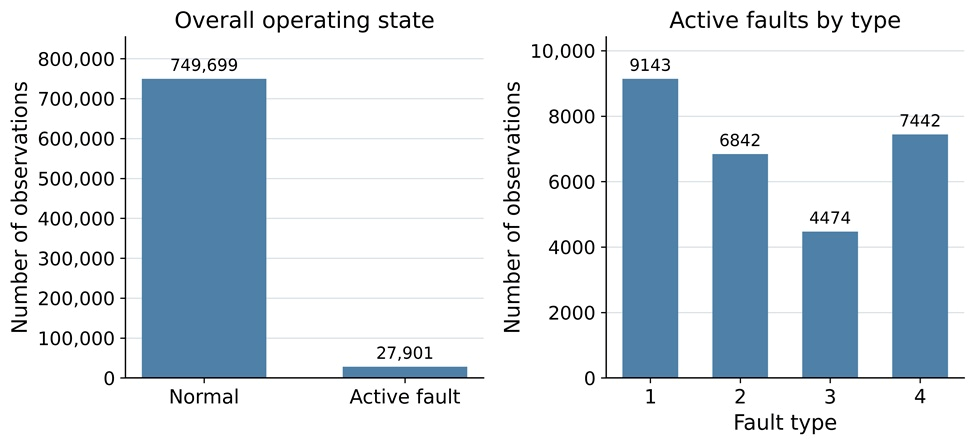
The original dataset contained 777,600 observations, of which 749,699 represented normal operation and 27,901 corresponded to active faults. Normal operation therefore accounted for 96.41% of the observations, whereas active faults represented only 3.59%, demonstrating a pronounced class imbalance. Among the active-fault observations, fault type 1 was the most frequent, with 9143 observations, followed by fault type 4 with 7442 observations, fault type 2 with 6842 observations, and fault type 3 with 4474 observations. The distributions of normal-operation and active-fault observations are presented in Figure 1.

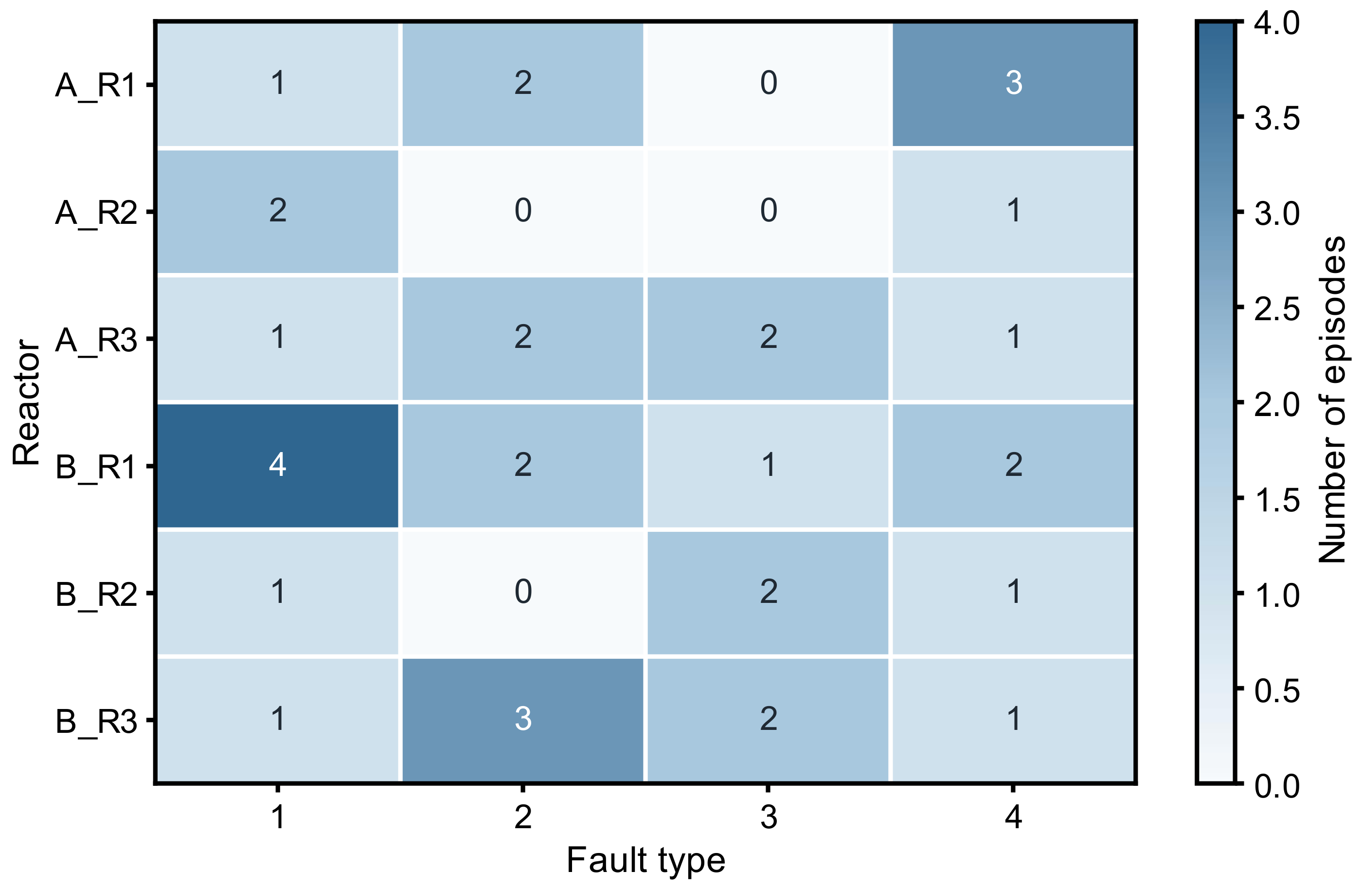
A total of 35 continuous fault episodes were identified, including ten episodes of fault type 1, nine episodes each of fault types 2 and 4, and seven episodes of fault type 3. Their durations ranged from 202 to 1417 min, with a median duration of 771 min. As shown in Figure 2, the episodes were not distributed uniformly across the six reactors. Fault types 1 and 4 occurred in all six reactors, whereas fault types 2 and 3 were represented in four reactors.

Missing values were present in all 16 continuous variables, with missing-value percentages close to 6%. By contrast, the timestamp, operating regime, reactor identifier, and fault-type variables contained no missing values. Consequently, temporal ordering, reactor identity, and fault-episode boundaries remained available for all observations.

For observations with a valid efficiency-loss target, normal operation was associated with zero efficiency loss. During active faults, the target ranged from approximately 5% to 25%, with a mean close to 15% for each fault type. The target values were distributed relatively evenly across the four efficiency-loss ranges. A monotonic progression was also observed within the analyzed fault episodes, generally increasing from approximately 5% to 25%. This regular behavior reflects the synthetic construction of the target and must be considered when interpreting the regression results.

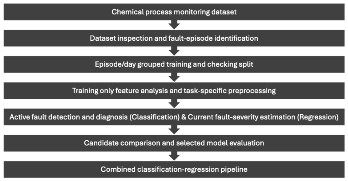
The complete methodological workflow, including dataset inspection, grouped partitioning, task-specific preprocessing, feature selection, model comparison, grouped cross-validation, and integrated pipeline evaluation, is summarized in Figure 3.

The grouped partitioning strategy produced a raw training partition of 624,024 observations and a checking partition of 153,576 observations. The fault-episode allocation consisted of 27 training episodes and eight checking episodes, including two checking episodes from each fault type. Normal operation was divided into 72 training dates and 18 checking dates.

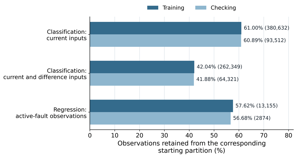
To avoid unnecessary loss of observations, missing-value removal was performed separately for each modeling task according to its required inputs and target. As illustrated in Figure 4, the training and checking partitions retained similar percentages of observations, while all 35 fault episodes remained represented. The greatest reduction occurred for classification with one-minute differences because these features additionally required valid consecutive observations.

3.2. Exploratory Fault Patterns and Feature Evidence

Feature analysis was performed exclusively on the training partitions. The examined criteria included one-way analysis of variance, effect size, mutual information, Pearson correlation, fault-specific correlations, and inter-feature redundancy. These complementary measures were interpreted together because no individual statistic could represent every linear, nonlinear, and fault-specific relationship contained in the data.

For classification, vibration RMS produced the largest ANOVA effect size, at 0.609, followed by conversion rate at 0.412 and motor current at 0.184. These variables provided the clearest overall separation among normal operation and the four fault classes. Mutual-information analysis supplied additional evidence for variables with nonlinear relationships, with ambient temperature effect producing the highest-classification mutual information score of 0.084.

For regression, the eight retained variables were also the eight highest-ranked candidates according to mutual information. Their scores ranged from 0.095 for temperature error to 0.590 for vibration RMS. Several variables exhibited stronger nonlinear or fault-specific relationships than their overall Pearson correlations suggested. For example, ambient temperature effect had an overall correlation of only 0.002 with efficiency loss but a mutual information score of 0.476. These findings supported the combined use of statistical relevance, fault-specific behavior, redundancy analysis, and process interpretation in selecting the final inputs.

The analysis also identified redundant candidate variables. Operating regime, temperature setpoint, and pressure setpoint were perfectly correlated in the classification training data, while reactor temperature and reaction rate exhibited a correlation of approximately 0.999. Excluding redundant alternatives reduced duplication while retaining measurements with useful statistical and process-related information.

The selected variables represented different types of fault behavior. Fault type 1 was primarily characterized by increased temperature error and reduced coolant flow. Fault type 2 was associated with reduced feed flow and conversion rate, while fault type 3 was predominantly characterized by temperature-related changes. Fault type 4 produced increased vibration RMS and motor current. These relationships were descriptive of the synthetic dataset and were not interpreted as evidence of causal mechanisms or as predefined fault patterns that would necessarily generalize to a real chemical process.

3.3. Classification Model Comparisons

The always-normal dummy achieved high accuracy because normal operation dominated the dataset, but it provided no fault detection capability. This result confirmed that accuracy alone was not suitable for model selection. Logistic regression, Random Forest and the ANN produced comparable overall performance. The ANN slightly improved balanced accuracy and fault recall, whereas logistic regression produced higher alarm precision and fewer false alarms. Class-specific examination showed that none of these models identified fault type 3, indicating that nonlinear modeling alone did not resolve the most difficult class. Changes in network size and activation function provided no clear improvement. Class balancing increased sensitivity at the cost of substantially more false alarms, while the two-stage approach offered no clear overall benefit. The ANN model was therefore retained as the reference nonlinear configuration for the subsequent temporal and reactor-information experiments. The corresponding aggregate and operational metrics are presented in

Table 1. Classification model comparisons on the current-input checking partition.

Configuration	Accuracy (%)	Balanced Accuracy (%)	Macro F1 (%)	Fault Recall (%)	Alarm Precision (%)	False Alarms per 1000 Normal Observations
Always-normal dummy	96.72	20.00	19.67	0.00	N/A	0.000
Multinomial logistic regression	98.88	67.63	72.54	66.23	99.32	0.155
Random forest classifier	98.45	67.45	71.57	65.87	83.44	4.434
ANN (64, 32), ReLU	98.79	68.27	72.30	67.34	94.04	1.448
Smaller architecture (32, 16)	98.78	67.76	72.23	66.46	95.01	1.183
Larger architecture (128, 64)	98.75	67.20	71.87	65.71	94.51	1.294
Tanh activation (64, 32)	98.79	68.15	72.53	67.08	94.53	1.316
Mild balancing	98.52	67.66	70.81	66.72	84.97	4.002
Moderate balancing	97.06	67.85	67.94	67.89	54.36	19.338
Full balancing	80.86	66.89	44.80	80.87	12.80	186.856
Two-stage classification	98.76	67.12	71.72	65.48	95.39	1.072

.

The controlled comparison showed that adding one-minute differences improved multiclass performance and fault recall without increasing the false-alarm frequency. However, temporal information alone did not enable the model to identify fault type 3. Adding reactor identity produced the largest overall improvement and increased fault type 3 recall from 0% to 31.75%, while alarm precision and false-alarm performance were maintained. These findings indicate that short-term process changes and equipment-specific context provided complementary information within the six-reactor synthetic dataset. Because fault type 3 was unevenly distributed across reactors, part of the improvement associated with reactor identity may reflect differences in fault prevalence rather than equipment-specific process behavior alone.

Table 2. Controlled comparison of current measurements, one-minute differences, and reactor identity on the delta-valid checking partition.

Configuration	Balanced Accuracy (%)	Macro F1 (%)	Fault Recall (%)	Alarm Precision (%)	False Alarms per 1000 Normal Observations	Fault Type 3 Recall (%)
Current inputs on delta-valid rows	67.32	71.98	65.56	96.43	0.820	0.00
Current and difference inputs	70.80	74.37	70.98	96.69	0.820	0.00
Current and difference inputs with reactor identity	76.25	82.44	75.59	97.01	0.788	31.75

presents this controlled comparison, using the current-input model evaluated on the same delta-valid observations as the reference.

The configurations reported in Table 1 and Table 2 were evaluated on different checking partitions and should not be compared directly. Comparisons within each table were made using identical observations. Based on the controlled comparison in Table 2, the configuration containing the eight current measurements, six one-minute differences, and reactor identity was retained as the selected classifier.

3.4. Selected Classifier Performance

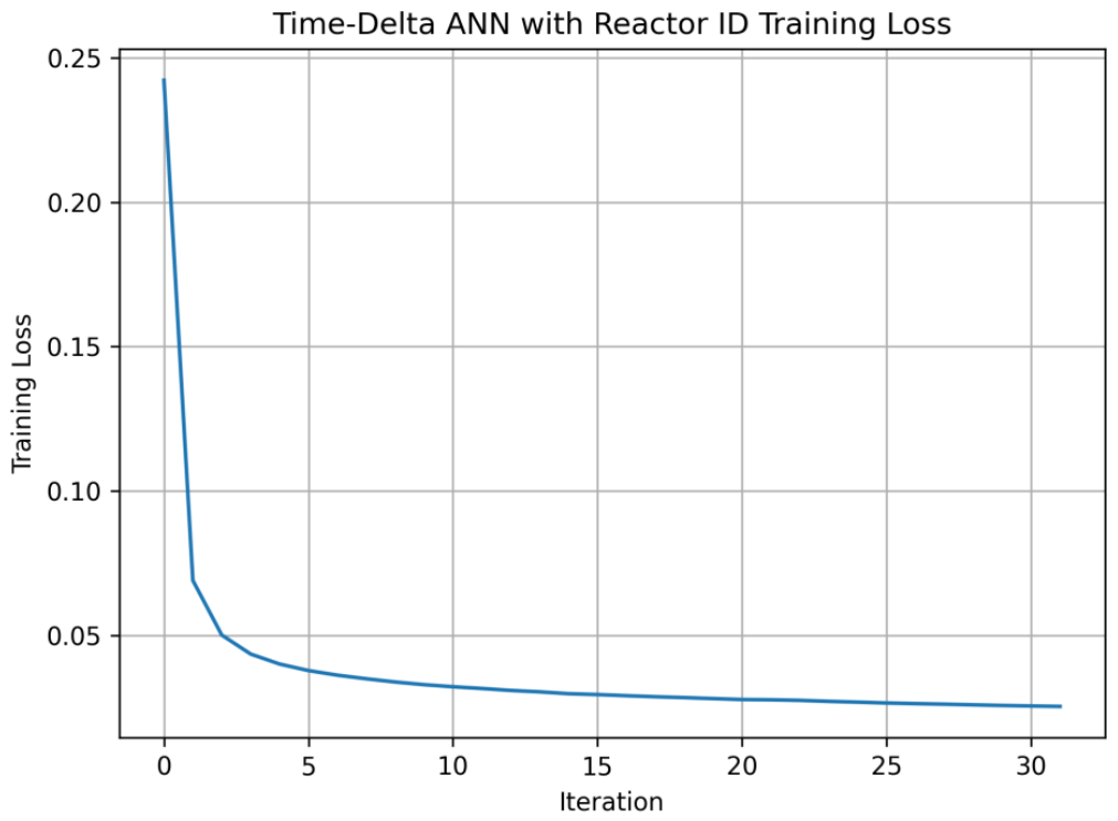
The selected classifier completed 32 training iterations under the early-stopping procedure. Training loss decreased from 0.242 during the first recorded iteration to 0.025 during the final iteration. The most pronounced reduction occurred during the initial stage of training, followed by smaller improvements as the model approached convergence, as shown in Figure 5.

The classifier was evaluated on 64,321 delta-valid checking observations, including 62,219 normal observations and 2102 active-fault observations. It achieved an overall accuracy of 99.09%, balanced accuracy of 76.25%, and macro F1-score of 82.44%. Macro precision and macro recall were 91.99% and 76.25%, respectively. The large difference between ordinary and balanced accuracy reflects the predominance of normal observations. Balanced accuracy therefore provides the more representative assessment and indicates moderate, rather than uniformly strong, performance across the five classes.

For the normal-versus-fault decision, the selected model detected 75.59% of the active-fault observations and achieved an alarm precision of 97.01%. Only 49 of the 62,219 normal observations were incorrectly assigned to a fault class. This corresponded to a false-alarm rate of 0.0788%, or approximately 0.788 false alarms per 1000 normal observations.

Class-specific performance is reported in

Table 3. Class-specific performance of the selected classifier on the checking partition.

Class	Precision (%)	Recall (%)	F1-Score (%)	Observations
Normal operation	99.18	99.92	99.55	62,219
Fault type 1	97.36	68.53	80.44	699
Fault type 2	100.00	91.19	95.39	772
Fault type 3	64.10	31.75	42.46	315
Fault type 4	99.30	89.87	94.35	316

. Fault types 2 and 4 were identified most reliably, while fault type 1 achieved intermediate performance. Fault type 3 remained the principal limitation, as its low recall indicates that most observations from this class were not correctly identified.

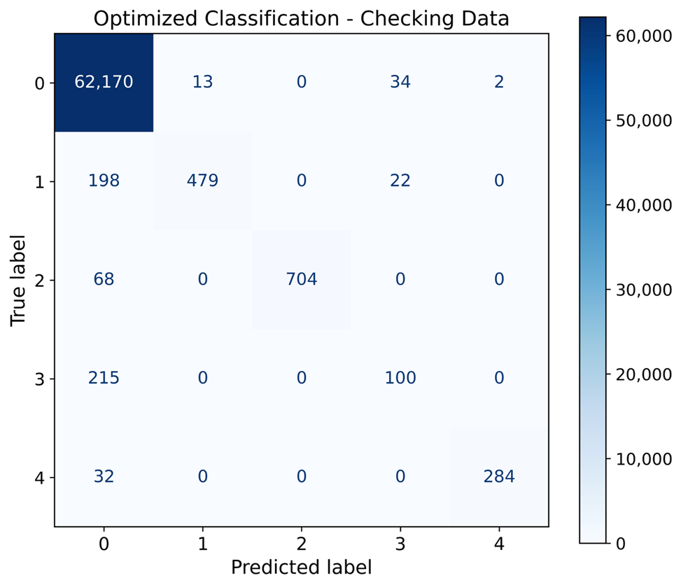
The corresponding confusion matrix is presented in Figure 6. Most errors involving active faults were missed detections assigned to normal operation rather than incorrect assignments among the fault categories. In total, 513 active-fault observations were classified as normal. A further 22 observations from fault type 1 were assigned to fault type 3, whereas no other cross-fault misclassifications occurred. Fault type 3 accounted for the largest proportion of missed detections, with 215 of its 315 observations classified as normal.

3.5. Episode-Level Classification and Feature Importance

Episode-level evaluation showed that the model correctly detected at least some observations from all eight checking episodes. Nevertheless, performance varied substantially among episodes, including episodes belonging to the same fault type. The complete results are presented in

Table 4. Episode-level performance of the selected classifier on the checking partition.

Episode	Reactor	Fault Type	Observations	Fault Detection Recall (%)	Correct Fault-Type Rate (%)
2	A_R1	2	370	88.11	88.11
9	B_R1	1	562	77.40	73.49
10	A_R3	3	168	51.19	51.19
13	A_R3	2	402	94.03	94.03
21	B_R1	4	175	89.14	89.14
27	B_R1	4	141	90.78	90.78
31	B_R1	1	137	48.18	48.18
34	B_R2	3	147	9.52	9.52
Observation-weighted overall	—	All	2102	75.59	74.55
Episode-equal mean (95% CI)	—	All	—	68.54 (48.25–85.90)	68.05 (47.76–85.60)

.

Fault types 2 and 4 were detected consistently across their checking episodes, whereas fault type 1 showed a wider difference between incidents. Fault type 3 was both the weakest and least stable, with detection performance changing substantially between its two episodes. These results show that a single fault-type score can conceal incident-specific model behavior.

For seven of the eight checking episodes, fault detection recall and correct fault-type rate were identical because all detected observations were assigned to the correct fault category. Episode 9 was the only exception, as some detected fault type 1 observations were classified as fault type 3. Giving each episode equal weight produced a more conservative assessment because shorter and more difficult episodes were no longer given less influence than longer episodes. The wide confidence intervals also indicate substantial variation among the eight checking episodes.

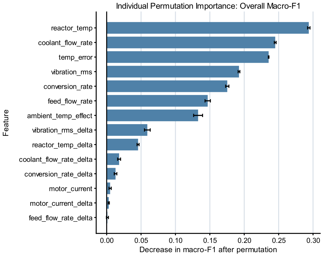
Permutation analysis was used to examine the selected classifier’s dependence on its 14 continuous inputs. As shown in Figure 7, permuting reactor temperature produced the largest mean reduction in macro F1-score, at 0.294. It was followed by coolant flow rate at 0.245, temperature error at 0.235, vibration RMS at 0.192, and conversion rate at 0.175.

Current measurements generally produced larger individual reductions in macro F1-score than their corresponding difference features. Among the temporal inputs, the vibration RMS difference produced the largest reduction, followed by the reactor-temperature difference. Their comparatively smaller individual importance does not contradict the controlled improvement reported in Table 2 because the six difference features were introduced collectively and may have provided complementary or overlapping information.

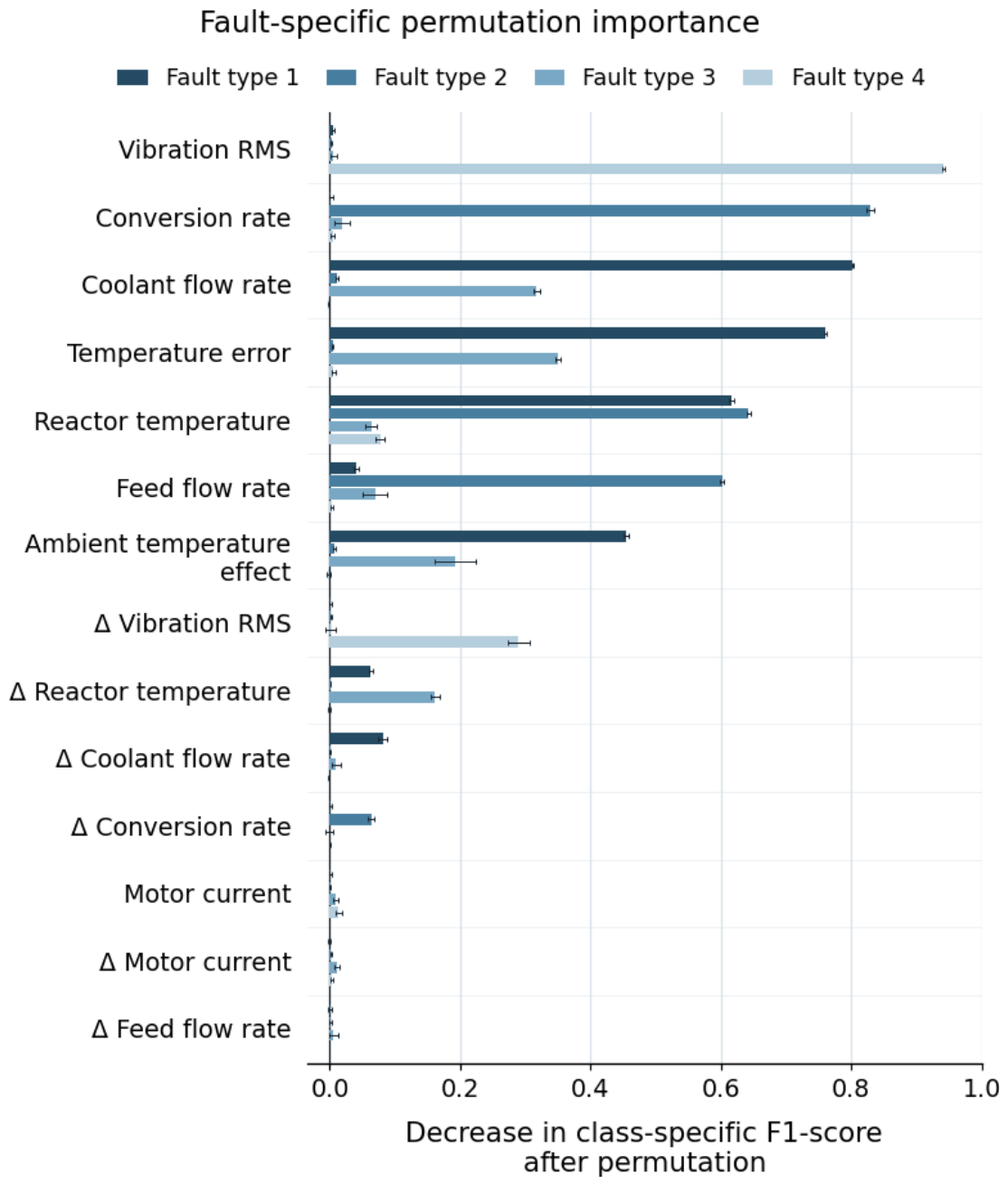
The fault-specific permutation analysis in Figure 8 further showed that the relative importance of individual variables differed among fault categories. Fault type 1 depended mainly on coolant flow rate, temperature error, and reactor temperature. Fault type 2 depended most strongly on conversion rate, reactor temperature, and feed flow rate. Temperature error and coolant flow rate were the most influential inputs for fault type 3, whereas fault type 4 depended primarily on vibration RMS and its one-minute difference.

The permutation results represent the model’s dependence on the fitted inputs rather than causal effects. In addition, correlated measurements may share predictive information, meaning that a limited individual permutation effect does not necessarily indicate that the corresponding variable contains no useful information.

3.6. Grouped Cross-Validation of the Classifier

Five-fold grouped cross-validation was performed using all available delta-valid observations. Complete fault episodes and grouped normal-operation days were assigned to individual folds, preventing observations from the same group from appearing in both the training and validation portions of a fold. The validation folds contained between 64,988 and 65,637 observations and between six and eight fault episodes.

Table 5. Five-fold grouped cross-validation results for the selected classifier.

Metric	Mean (%)	Standard Deviation (%)	Minimum (%)	Maximum (%)
Accuracy	98.88	0.14	98.74	99.09
Balanced accuracy	74.84	4.19	68.53	79.68
Macro F1-score	79.80	5.07	71.61	83.97
Fault type 1 recall	58.60	9.88	43.20	66.34
Fault type 2 recall	89.43	2.92	85.69	93.56
Fault type 3 recall	38.22	23.89	0.00	56.59
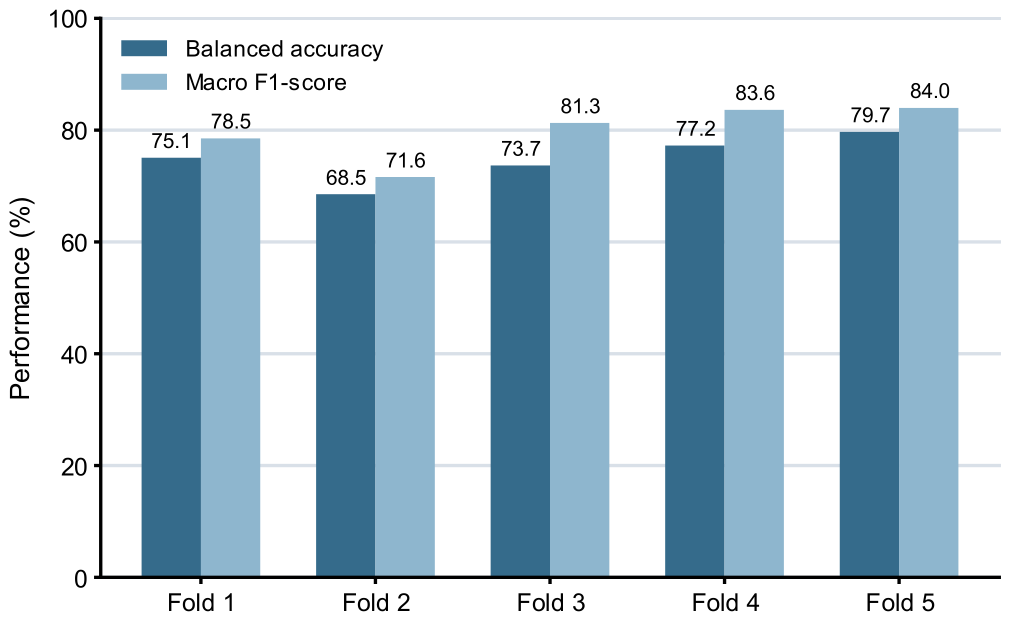
Fault type 4 recall	88.03	4.16	82.15	92.26

summarizes the mean performance, variability and observed range. Overall accuracy remained stable, whereas balanced accuracy and macro F1-score were more sensitive to fold composition.

Figure 9 shows that balanced accuracy and macro F1-score followed a similar pattern across the five folds, indicating that model performance depended on the fault episodes included in each fold.

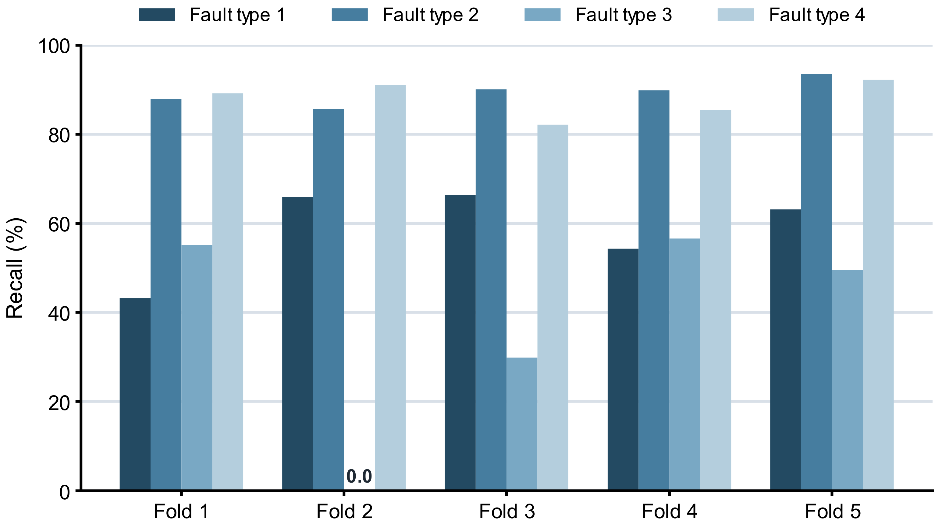
Fault-specific recall across the five folds is presented in Figure 10. Fault types 2 and 4 remained consistently well identified, while fault type 1 showed moderate differences across folds. Fault type 3 was the least stable and was not detected in one-fold, making it the main source of variation in the aggregate results.

These findings supported the principal checking-partition results while showing that the classification of fault type 3 depended strongly on the specific fault episodes assigned to evaluation.

3.7. Regression Model Comparison

The regression reference models and the sensor-only ANN configurations were evaluated using the same 2874 active-fault checking observations. The training-median model provided a minimum reference, while the elapsed-time baseline used only the minutes from the actual labeled episode onset. Ridge regression, Random Forest, and the ANN configurations used the eight selected current process measurements without reactor identity or fault-type information.

The training-median model did not explain the variation in efficiency loss. In contrast, the elapsed-time baseline achieved meaningful predictive performance, indicating that the structured within-episode progression contributed to target predictability. However, its performance remained below the sensor-based Ridge and ANN 64/32 models, showing that elapsed time alone did not account for their complete predictive performance. Ridge regression produced the strongest R² and RMSE results in the current-input comparison. Among the nonlinear models, the ANN 64/32 performed better than the Random Forest in R², MAE, and RMSE, whereas the Random Forest produced a lower median absolute error. The smaller ANN achieved the lowest MAE and median absolute error, showing that the relative comparison depended partly on the error measure considered. Increasing network size provided no benefit. The complete results are presented in

Table 6. Comparison of regression models and sensor-based models on the checking partition.

Model	Architecture	R2	MAE	RMSE	Median Absolute Error	Training Iterations
Training-median model	—	−0.000	5.028	5.801	5.080	—
Elapsed-time-only regression	Linear, one input	0.509	3.017	4.066	2.334	—
Ridge regression	Linear	0.607	2.595	3.634	1.932	—
Random Forest regressor	300 trees	0.539	2.554	3.937	1.378	—
ANN 64/32	(64, 32)	0.575	2.478	3.779	1.614	477
ANN 32/16	(32, 16)	0.565	2.298	3.827	1.280	747
ANN 128/64	(128, 64)	0.482	2.634	4.175	1.498	534

.

Although Ridge regression achieved slightly higher performance than the sensor-only ANN configuration, the ANN architecture was retained for subsequent experiments because it provided a flexible nonlinear framework that could consistently incorporate additional contextual inputs, including reactor identity and fault-type information. The objective of the study was therefore not to establish ANN superiority over all alternatives but to examine how contextual information affects severity estimation within a unified modeling framework.

3.8. Effects of Reactor Identity and Fault-Type Information

The contribution of reactor identity and fault-type information was examined using the ANN 64/32 architecture and the same 2874 checking observations. The inclusion of either input improved the performance of the sensor-only regression model. Although the two configurations achieved similar R² values, the use of actual fault-type information resulted in lower prediction errors. The combination of reactor identity and actual fault type produced the strongest performance across all evaluation metrics, indicating that equipment-specific and fault-specific context provided additional predictive information within this dataset. Since reactor identity improved performance even when the actual fault type was provided, the results suggest that reactor-specific contextual information may contribute to efficiency-loss estimation. However, this improvement may also reflect differences in fault prevalence or other dataset-specific associations that cannot be disentangled using the available data.

Table 7. Effect of reactor identity and actual fault-type information on regression performance.

Inputs	R2	MAE	RMSE	Median Absolute Error	Training Iterations
Sensor variables	0.575	2.478	3.779	1.614	477
Sensors and reactor identity	0.849	1.700	2.254	1.354	282
Sensors and actual fault type	0.849	1.417	2.257	0.856	235
Sensors, reactor identity and actual fault type	0.920	1.146	1.637	0.801	143

summarizes the controlled comparison.

Configurations containing the actual fault type constitute oracle evaluations because the correct diagnostic label was supplied directly to the regression model. Accordingly, these results do not represent the information that would necessarily be available during real-time operation.

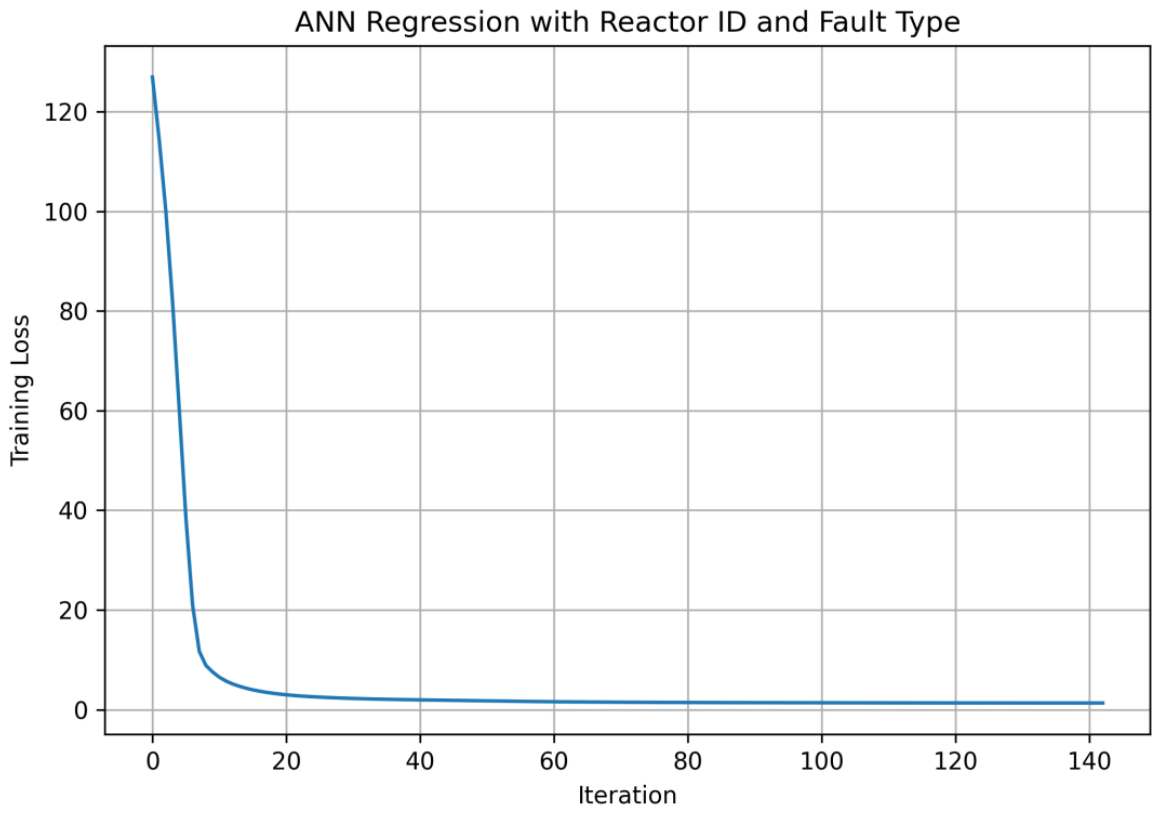
The selected regression model completed 143 training iterations before the early-stopping criterion was satisfied. Its loss decreased rapidly during the initial iterations and then improved more gradually, as shown in Figure 11.

3.9. Selected Regression Model Performance

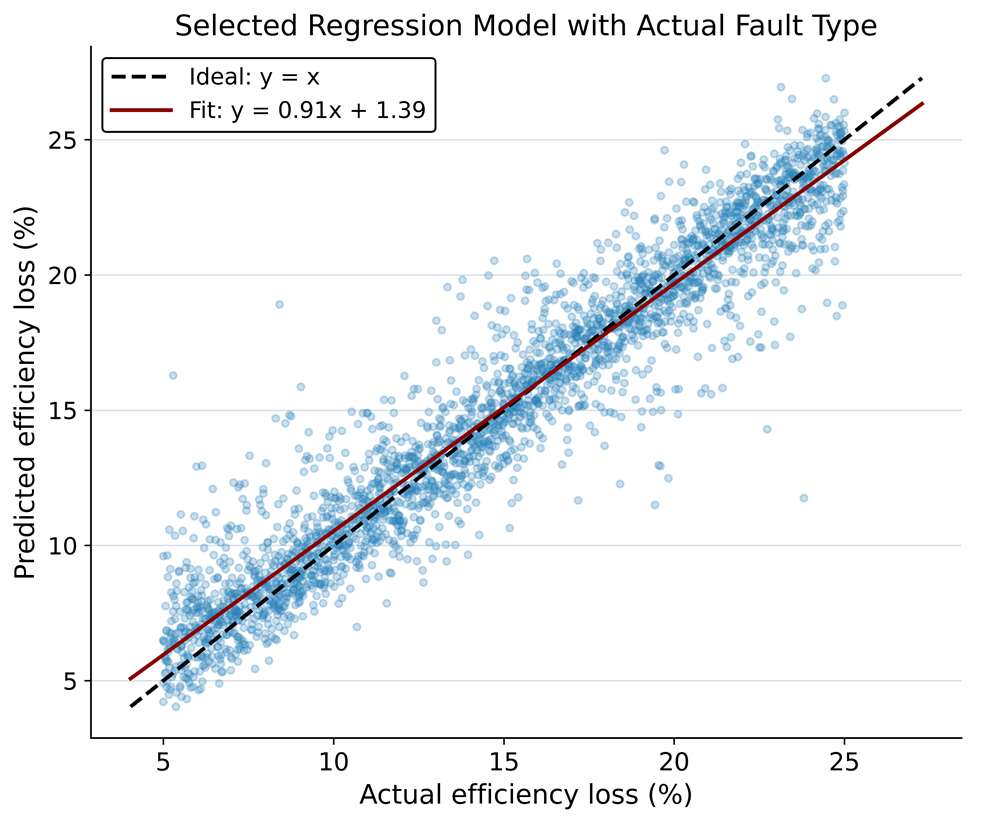
The selected regression model was evaluated using the actual fault type for all 2874 active-fault checking observations. Under this oracle condition, it achieved an R² of 0.920, an MAE of 1.146 percentage points, and an RMSE of 1.637 percentage points. These results provide a reference for the regression performance obtained when the correct fault diagnosis is available. They do not represent the complete operational pipeline, where the fault type is supplied by the classifier.

The relationship between the actual and predicted efficiency-loss values is presented in Figure 12. Most observations were distributed close to the ideal diagonal, although greater dispersion occurred for some target values. The fitted relationship was $y = 0.91x + 1.39$, indicating a tendency to slightly overestimate lower losses and underestimate higher losses.

Performance varied across fault categories, as reported in

Table 8. Performance of the selected regression model by fault type.

Fault Type	Episodes	Observations	R2	MAE	RMSE
1	2	938	0.906	1.417	1.777
2	2	1071	0.981	0.652	0.797
3	2	438	0.752	2.295	2.947
4	2	427	0.982	0.609	0.774

. Fault types 2 and 4 produced the most accurate estimates, while fault type 1 also maintained comparatively strong performance. Fault type 3 remained the principal limitation, with weaker model fit and larger prediction errors. These differences show that the overall regression metrics did not represent every fault condition equally. MAE and RMSE are expressed in efficiency-loss percentage points.

3.10. Regression Cross-Validation and Feature Importance

The selected regression model was further evaluated using five-fold episode-grouped cross-validation. Complete fault episodes were assigned to individual folds, preventing observations from the same episode from appearing in both the training and validation portions of a fold. The actual fault type was supplied during cross-validation; therefore, the results assess the stability of the selected oracle regression configuration rather than the complete classification–regression pipeline.

Episode-grouped cross-validation produced relatively stable regression performance, and the fixed checking-partition results remained within the ranges observed across the five folds.

Table 9. Episode-grouped cross-validation results for the selected regression model.

Metric	Mean	Standard Deviation	Minimum	Maximum
R2	0.892	0.018	0.878	0.928
MAE	1.320	0.163	1.043	1.520
RMSE	1.894	0.170	1.558	2.030

summarizes the mean performance, variability and range. MAE and RMSE are expressed in efficiency-loss percentage points.

Fault-specific cross-validation results are presented in

Table 10. Mean episode-grouped cross-validation performance by fault type.

Fault Type	Mean R2	Minimum R2	Maximum R2	Mean MAE	Mean RMSE
1	0.887	0.771	0.927	1.542	1.900
2	0.974	0.933	0.990	0.702	0.868
3	0.658	0.486	0.757	2.653	3.340
4	0.968	0.911	0.992	0.761	0.939

. Fault types 2 and 4 produced the highest mean R² values and the lowest errors. Fault type 1 also produced comparatively strong performance but showed greater variation. Fault type 3 remained the most difficult condition. Mean MAE and mean RMSE are expressed in efficiency-loss percentage points.

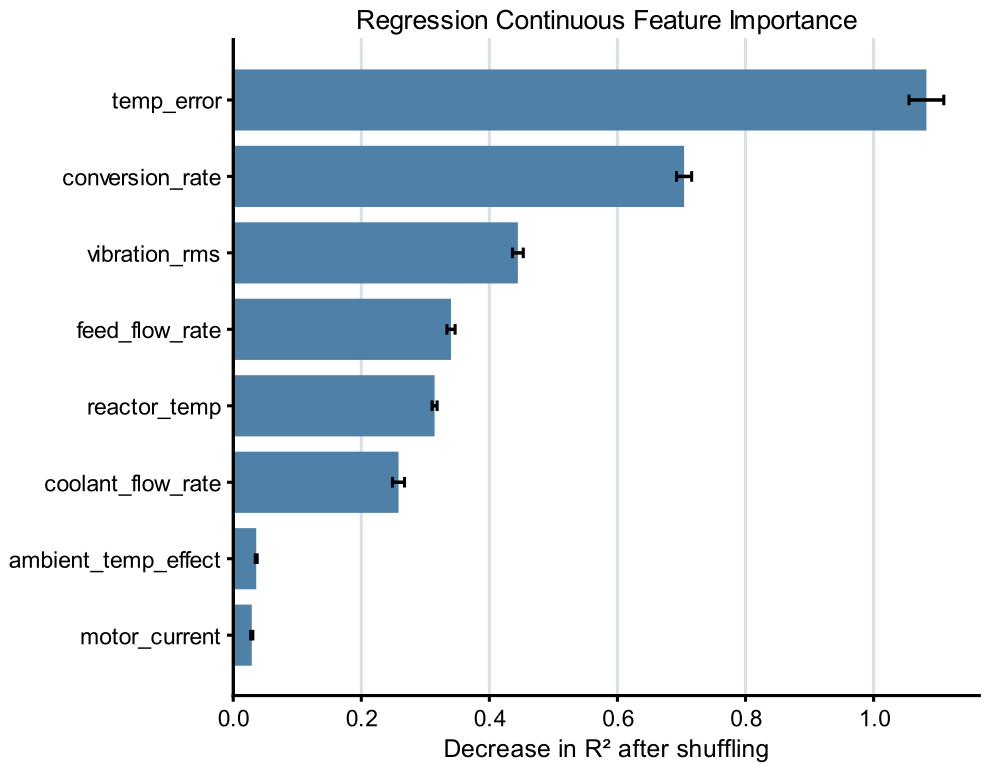
Permutation importance was applied to the eight continuous process measurements using the fixed checking partition. Temperature error, conversion rate and vibration RMS were identified as the variables with the strongest individual effects on R², as shown in Figure 13. Reactor identity and fault type were retained unchanged because their contributions had already been examined through the controlled model configurations.

The permutation results describe model dependence rather than causal influence. Correlated measurements may share predictive information, while independently shuffling one variable may create combinations that do not normally occur in the dataset.

3.11. Integrated Classification–Regression Process

The selected classifier and regression model were connected to evaluate their end-to-end operation. The analysis included all 64,321 observations in the classifier’s checking partition, comprising 62,219 normal and 2102 active-fault observations. A nonzero one-minute classifier prediction was treated as an alarm and activated the regression stage using the classifier-predicted fault type. When normal operation was predicted, the pipeline returned zero efficiency loss.

All active-fault observations were retained for detection and diagnosis measures. However, 133 active-fault observations did not have a valid efficiency-loss target. These observations were included when calculating detection recall but were excluded from the regression-error measures. The operational outcomes are summarized in

Table 11. Regression stage activation across the classifier’s checking partition.

Actual Operating Condition	Regression Not Activated	Regression Activated	Total
Normal operation	62,170	49	62,219
Active fault	513	1589	2102
Total	62,683	1638	64,321

.

The activation pattern shows that missed faults were more important to the complete process than false downstream activations because they prevented severity estimation from being performed. When the regression stage was activated, the classifier assigned the correct fault type in 98.62% of cases. The complete pipeline performance therefore depended mainly on fault detection coverage rather than fault-type confusion after detection.

To identify how classification outcomes affected severity estimation, regression performance was examined under different conditions. The selected regressor was evaluated using the detected active faults observations using the actual fault type. The same observations were then evaluated using the classifier-predicted fault type, isolating the effect of diagnostic errors. The evaluation was subsequently extended to all active-fault observations with valid targets, with zero efficiency loss assigned when the classifier missed a fault. False activations during normal operation and performance across the complete partition were also examined. The results are presented in

Table 12. Severity estimation under different pipeline conditions.

Pipeline Condition	Evaluation Scope	Observations	R2	MAE	RMSE
Actual fault type	Detected active faults	1487	0.932	0.968	1.315
Classifier-predicted fault type	Detected active faults	1487	0.906	1.039	1.542
Complete pipeline	All valid target active faults	1969	0.153	3.110	5.376
Complete pipeline	False activated normal observations	49	N/A	11.972	12.360
Complete pipeline	All observations	64,188	0.871	0.105	1.002

, with MAE and RMSE expressed in efficiency-loss percentage points.

Replacing the actual fault type with the classifier prediction caused only a moderate reduction in performance. A much larger deterioration occurred when missed faults were included, as these observations did not activate the regressor and received an output of zero. False alarms were infrequent but produced nonzero efficiency loss during normal operation, demonstrating their downstream effect. Although performance across all observations appeared strong, it was dominated by correctly identified normal operation. Complete pipeline performance therefore depended mainly on reliable fault detection.

The fault-specific end-to-end results are presented in

Table 13. Complete-process performance by fault type.

Fault Type	Detected/Common	Detection (%)	Correct Type Among Detected (%)	R2	MAE	RMSE
1	470/654	71.87	95.32	0.305	3.502	4.965
2	660/725	91.03	100.00	0.887	1.121	1.943
3	93/296	31.42	100.00	−2.446	9.016	11.141
4	264/294	89.80	100.00	0.855	1.195	2.114

. Fault types 2 and 4 retained strong complete process performance because most of their active-fault observations were detected, while fault type 1 showed lower coverage. Fault type 3 remained the principal limitation. The negative R² for fault type 3 indicated performance below a mean-value estimate, mainly because missed faults were assigned zero efficiency loss.

Since fault episodes differed in duration, a separate episode-equal analysis was performed to prevent longer episodes from having greater influence on the overall results. The comparison with the observation-weighted evaluation is presented in

Table 14. Observation-weighted and episode-equal regression performance of the complete pipeline on active-fault checking observations with valid efficiency-loss targets.

Evaluation Approach	Evaluation Scope	R2	MAE	RMSE
Observation-weighted complete pipeline	1969 observations	0.153	3.110	5.376
Episode-equal complete pipeline (95% confidence intervals)	8 episodes	−0.222 (−1.676–0.727)	3.972 (1.690–6.917)	5.131 (2.627–8.269)

.

The episode-equal results provide a less favorable assessment of the complete pipeline when every incident is given the same importance. The negative mean R² indicates that performance was particularly weak in some episodes, primarily because missed faults resulted in zero severity estimates. However, the relatively small change in RMSE shows that the effect of equal weighting was not uniform across all error measures. The wide confidence interval for R², which includes zero, further demonstrates the substantial uncertainty associated with the limited number and variable difficulty of the checking episodes.

Overall, the regression model generally estimated efficiency loss accurately when an active fault was detected and correctly diagnosed. Incorrect diagnostic labels caused a moderate reduction among detected observations, whereas missed faults prevented regression activation and had a much larger effect. Complete-process performance therefore depended mainly on detection coverage, particularly for fault type 3.

4. Discussion

The results demonstrate that the examined process measurements contain sufficient information to support both fault diagnosis and fault severity estimation within the synthetic multi-reactor process. The proposed framework successfully combined classification and regression models to provide complementary information regarding process condition and operational degradation. While the classification task focused on identifying active faults and distinguishing among fault categories, the regression task quantified the associated efficiency loss, thereby extending the monitoring capability beyond conventional fault diagnosis. Overall, the findings indicate that integrating these two functions can provide a more comprehensive assessment of process health than either task alone.

The main contribution of this study is the controlled, episode-aware evaluation of fault diagnosis and current efficiency-loss estimation as connected monitoring tasks. Rather than reporting classification and regression performance in isolation, the experiments examined how temporal and contextual inputs affected each stage and how classification outcomes influenced downstream severity estimation. The procedure separated oracle regression performance, diagnostic error and missed pipeline activation.

The classification experiments revealed that fault recognition performance varied considerably among the four fault types. Fault types 2 and 4 consistently achieved high recall and F1-scores, suggesting that their process patterns were well represented by the selected features. In contrast, fault type 3 remained substantially more difficult to detect, both in the fixed checking partition and during grouped cross-validation. This behavior is likely associated with the more subtle and partly overlapping temperature-related patterns characterizing this fault category. Importantly, most classification errors corresponded to missed detections that were assigned to normal operation rather than misclassifications among fault types. Consequently, the principal challenge was recognizing the presence of an abnormal condition rather than distinguishing between alternative fault categories once a fault had been detected.

The experiments further demonstrated the value of incorporating short-term temporal information into the diagnostic process. The addition of one-minute difference features improved balanced accuracy, macro F1-score, and fault detection recall without substantially increasing false alarms. These findings suggest that fault-related dynamics are not fully captured by instantaneous measurements alone. By representing short-term changes in process variables, the temporal features provided additional information regarding the evolution of process conditions and enabled more effective discrimination between normal and abnormal behavior without requiring a sequence-model architecture. Nevertheless, the performance gains were accompanied by a reduction in the number of observations eligible for classification, since the difference features required the availability of consecutive measurements. This trade-off should be considered in practical deployments where missing data and communication interruptions may be common.

Reactor identity emerged as one of the most influential sources of contextual information. However, this improvement may reflect both equipment-specific context and differences in fault prevalence, since fault types were not represented equally across the reactors. Its inclusion produced substantial improvements in both classification and regression performance, indicating that the relationship between sensor measurements and process condition differed across the six simulated reactors. These findings suggest that equipment-specific characteristics influence how faults manifest themselves in the observed process variables. At the same time, the strong contribution of reactor identity highlights a potential limitation regarding model transferability. Because all reactors were represented during training, the reported results reflect the ability of the models to generalize to new operating episodes of known equipment rather than to entirely unseen reactors. Future studies should therefore investigate unseen or matched reactors with comparable fault-type coverage and operating conditions.

The severity estimation results showed that process measurements alone provided meaningful predictive information regarding efficiency loss, as evidenced by the performance of both Ridge regression and the sensor-only neural network models. However, the most substantial improvements were achieved when reactor identity and fault-type information were incorporated into the regression framework. The selected model achieved its strongest performance when both sources of contextual information were available, demonstrating that severity estimation depends not only on the current process state but also on the specific operating context in which the observations occur. Different fault categories exhibited distinct relationships between process variables and efficiency degradation, making fault-type information particularly valuable for accurate prediction. The results therefore indicate that context awareness may be as important as sensor information for fault severity estimation in this synthetic industrial process.

The evaluation of the combined classification–regression process provided important insights into the interaction between fault diagnosis and severity estimation. When the regression model received classifier-predicted fault types, its performance decreased only moderately compared with the oracle scenario in which the actual fault labels were supplied. In contrast, the inclusion of missed faults produced a pronounced deterioration in overall process performance. This finding demonstrates that the effectiveness of the complete monitoring framework depends primarily on reliable fault detection. Once a fault is successfully detected, diagnosis errors have a comparatively smaller influence on severity estimation. All eight checking episodes were detected. Consequently, future developments should prioritize improving fault detection coverage, particularly for challenging fault categories such as fault type 3. This analysis moves the evaluation beyond isolated classification and regression measures by showing how errors from the first stage affect the output of the second.

The grouped cross-validation analyses generally supported the findings obtained from the fixed checking partition. Classification and regression performance remained comparable across grouped episode allocations, providing stability evidence but not independent external validation. Nevertheless, considerable variability was observed for fault type 3, indicating that the characteristics of individual fault episodes can strongly influence predictive performance. This observation highlights the importance of episode-aware validation methodologies when evaluating industrial fault-monitoring systems.

Despite the encouraging results, several limitations should be acknowledged. The study was conducted using a synthetic dataset that does not fully reproduce the complexity, noise characteristics, and operational variability observed in real industrial facilities. The efficiency-loss target followed a highly structured progression within fault episodes, potentially simplifying the severity estimation task compared with real-world applications. The fixed checking partition was used during model comparison and was not a fully independent test set. The complete-pipeline single alarm was defined as a single nonzero one-minute prediction, and alternative persistence-based alarm criteria were not examined. The best-performing regression model relied on fault-type information that was available during training and oracle evaluation but may not always be perfectly known during deployment. Finally, the models were developed and evaluated using data from a limited set of reactors and operating conditions. These limitations suggest that the reported performance should be interpreted as evidence of methodological feasibility rather than as a direct estimate of expected industrial performance.

Overall, the study demonstrates the potential of combining machine learning-based fault diagnosis and severity estimation within a unified monitoring framework. The findings show that integrating diagnostic and severity-related information can provide a more comprehensive assessment of process condition than either task alone. Beyond the reported predictive performance, the work highlights the importance of evaluating monitoring systems at multiple levels, including fault-specific, episode-level, and end-to-end operational perspectives. Such analyses provide insights that may not be evident from aggregate performance metrics alone and help identify the factors that most strongly influence practical system behavior. The proposed framework therefore offers a structured approach for investigating the interaction between fault diagnosis and severity estimation within this synthetic industrial process-monitoring environment, while also providing a foundation for future studies using real-world data and more diverse operating conditions.

5. Conclusions

This study presented an integrated machine learning framework for fault detection, fault diagnosis, and fault severity estimation using time-series data obtained from a synthetic multi-reactor chemical process. The proposed framework combined classification and regression models to provide both categorical fault information and continuous estimates of efficiency degradation. The adopted evaluation methodology incorporated fault-episode-aware partitioning, grouped cross-validation, episode-level analysis, and leakage-mitigation procedures to support a more realistic assessment of monitoring performance across previously unseen fault episodes of known fault types.

The results demonstrated that the selected process measurements contained sufficient information to support effective fault monitoring within the synthetic benchmark environment. For fault diagnosis, the inclusion of temporal difference features and reactor identity improved performance while maintaining a low false-alarm rate. The findings also revealed substantial differences among fault categories, with fault type 3 proving considerably more difficult to identify than the remaining fault classes. These results highlight the importance of fault-specific analysis when evaluating industrial monitoring systems.

For severity estimation, the process variables provided meaningful predictive capability, while contextual information further improved performance. The inclusion of reactor identity improved classification and regression performance, although these gains cannot be attributed solely to equipment-specific process behavior. Reactor identity may encode both reactor-related operating context and differences in fault prevalence across reactors. Furthermore, severity estimation performance was substantially higher when accurate fault-category information was available, demonstrating the importance of the interaction between diagnosis and severity assessment within integrated monitoring frameworks.

Evaluation of the complete classification–regression pipeline showed that overall system performance depended primarily on effective fault detection. Missed faults had a considerably larger impact on end-to-end severity estimation than fault-classification errors because they prevented activation of the regression stage. The additional episode-level analysis further demonstrated the influence of episode duration and event-specific variability on performance estimates, emphasizing the importance of evaluating industrial monitoring systems beyond observation-level metrics alone.

Overall, the study demonstrates the methodological feasibility of combining fault diagnosis and fault severity estimation within a unified machine learning framework. However, the findings should be interpreted within the context of a synthetic benchmark environment and should not be considered direct estimates of performance in real industrial applications.

Future research should focus on validation using real industrial datasets, including external testing under a wider range of operating conditions and fault scenarios. Additional work should investigate reactor-level generalization through evaluation using previously unseen equipment, as well as the use of advanced sequence-learning architectures, uncertainty-aware prediction methods, and transfer-learning strategies. Finally, extending the framework to support fault progression modeling, prognostics, and remaining useful life prediction could contribute to more comprehensive decision-support systems for predictive maintenance and industrial asset management.