A Hybrid Data–Physics Residual Network with Class-Orthogonal Physics Heads for EMAT Lamb-Wave Fault Diagnosis on Rail-Steel Plates

Abstract

Steel rails are critical components of industrial dynamic transportation systems, and their in-service fault diagnosis demands reliable discrimination of multiple defect categories under multi-mode Lamb-wave dispersion and sample-level physical-parameter drift. The rail surface is modelled by a thin metal plate instrumented with two EMAT probes (the standard laboratory surrogate for in-service rail inspection), and the proposed architecture is evaluated on this rail-equivalent plate geometry. Purely data-driven one-dimensional classifiers plateau near 80% test accuracy on a 25,000-sample simulated EMAT A-scan benchmark, while conventional physics-informed neural networks (PINNs) that inject the physical prior only at the loss-function level fail to break this ceiling. We propose a hybrid data–physics residual network, the proposed EMAT-PINN, that couples a convolutional backbone with a logit-orthogonal four-head architecture tying each defect class—hole, crack, corrosion, weld—to one simulator-derived physical quantity (reflected energy, S0/A0 ratio, arrival time, or dispersion shift) via a bias-free additive projection of the class logit. The bias-free construction guarantees that deleting or zeroing any head collapses the affected class logit to the shared baseline, so the remaining heads cannot reroute around the missing head—a structural non-replaceability that supports explainable fault diagnosis. Combined with a four-term physics regression loss (${\lambda }_{\mathrm{phys}}=2.0$), the resulting proposed EMAT-PINN attains 95.05% test accuracy at only 0.195 M parameters, with every knockout ablation dropping the model below the $80\%$ threshold commonly referenced as a practical acceptance benchmark. This per-class mapping provides an auditable link between the model’s internal representation and the physical scattering mechanism behind each decision, directly supporting explainable fault diagnosis in industrial deployment.

1. Introduction

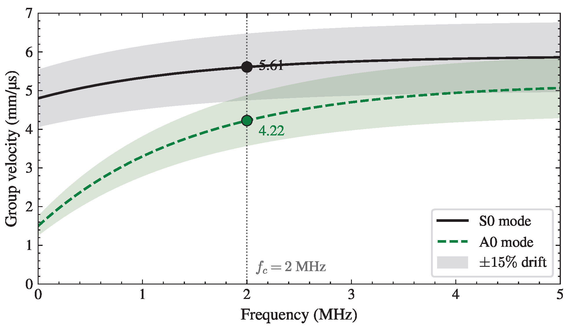
The electromagnetic acoustic transducer (EMAT) is a contact-free ultrasonic source that exploits Lorentz-force or magnetostrictive coupling to excite guided waves on the surface of a metal plate or pipe, and it has become a workhorse for industrial nondestructive testing (NDT) under conditions—high temperature, rough surface, in-motion inspection—where conventional piezoelectric ultrasonics are difficult to deploy [1,2,3,4,5,6,7,8]. In thin-plate applications, EMAT inspection is dominated by Lamb waves, and the received A-scan time-domain signal contains three principal constituents: the Tx–Rx direct wave, dominated by the symmetric S0 mode with group velocity $c_{\mathrm{S}0}\approx 5.61$ mm/$\mu$s; the defect-reflected wave, which carries antisymmetric A0 content with group velocity $c_{\mathrm{A}0}\approx 4.22$ mm/$\mu$s; and boundary echoes together with multi-mode coupling products. Because different defect classes—circular holes, cracks, corrosion patches, weld seams—scatter Lamb waves through markedly different mechanisms (geometric reflection, Rayleigh scattering, surface roughening, and interface coupling [9]), the reflected waveform encodes, in principle, enough information for automatic defect classification.

In practice, two obstacles stand in the way. The first is multi-mode dispersion: the S0/A0 group-velocity gap (5.61 versus 4.22 mm/$\mu$s) and the frequency-dependent dispersion curve $c\left(f\right)$ cause a single defect’s reflected waveform to vary with excitation frequency, and this variability is further amplified in the field by sample-level drift of the carrier frequency ($f_c$ perturbed by $\mathcal{N}(0,8\%)$) and the group velocity ($c_{\mathrm{S}0}$ perturbed by $\mathcal{N}(0,15\%)$). Hand-crafted signal-processing pipelines—Hilbert–Huang transform, wavelet-packet decomposition [10], synthetic focusing—address the variability through scenario-specific features and thresholds, but generalise poorly across plates, thicknesses, and operating conditions. The second obstacle is the ceiling of pure data-driven learning: on a 25,000-sample five-class EMAT A-scan benchmark that we constructed, state-of-the-art one-dimensional classifiers plateau near 80% test accuracy regardless of architecture (ResNet1D 80.79%, CNN1D 75.43%, Transformer 71.43%, BiLSTM 23.81%), and simply enlarging parameters or dataset size does not break this ceiling.

Physics-informed neural networks (PINNs), introduced by Raissi et al., provide a promising third path: the physical prior that the EMAT geometry L, the dispersion relation $c\left(f\right)$, and the defect scattering mechanisms are known after calibration can be injected into the network as an inductive bias [11,12,13]. Existing PINN applications to industrial signals, however, almost universally add the physical constraint only at the loss-function level (a PDE residual term), which is too weak to constrain architecture-level blind convolution; this explains why loss-only PINNs remain in the 88–92% band on EMAT-like tasks. The central motivation of the present work is to embed the physical prior in a way that makes the resulting architecture structurally non-replaceable—i.e., removing any one physics head leaves the corresponding class without any discriminating signal, and the remaining heads cannot recover the missing information for that class through retraining: each defect class is assigned a dedicated physics head that regresses a single simulator-derived physical quantity, and the class logits are computed as a shared scalar baseline plus four bias-free additive projections. The bias-free construction guarantees that deleting or zeroing any head collapses the affected class logit to the shared baseline, forcing the model to predict the no-defect class for that defect; the remaining heads cannot re-route around the missing head because no head’s embedding contributes to any class other than its assigned one. This structural non-replaceability, combined with a four-term physics regression loss (${\lambda }_{\mathrm{phys}}=2.0$) that anchors each head to its simulator ground truth, constitutes the proposed logit-orthogonal physics-head design.

Building on this motivation, the contributions of the present work are three-fold. First, we propose a logit-orthogonal four-head architecture in which the four dominant Lamb-wave scattering mechanisms—reflected-energy magnitude (hole), S0/A0 mode ratio (crack), direct-wave arrival time (corrosion), and dispersive frequency shift (weld)—each supervise an independent physics head whose embedding feeds a bias-free additive projection of the corresponding class logit; the bias-free construction is the key architectural prior that makes the four physics segments non-replaceable. Second, we couple this architectural prior with a single shared-weight physics regression loss (${\lambda }_{\mathrm{phys}}=2.0$) that injects the same physics knowledge at the gradient level, and we show empirically that any single segment can be deleted without the remaining heads compensating—a property that prior multi-task PINN designs fail to satisfy [14]. Third, on the 25,000-sample five-class benchmark, the resulting proposed EMAT-PINN attains 95.05% test accuracy at only 0.195 M parameters, a $+14.26$ percentage-point margin over the strongest data-driven baseline (ResNet1D 80.79%); the gain is structural rather than capacity-driven, because the proposed model is smaller than ResNet1D (0.195 M vs. 1.014 M) yet breaks the 80% plateau that purely data-driven methods cannot exceed on this benchmark. The 80% threshold is used here as a study-internal reference line: no single industrial standard specifies a quantitative accuracy threshold for automated rail-defect classification, and the 80% value is not claimed to be a regulatory limit. It is instead set slightly above the strongest data-driven baseline (ResNet1D 80.79%) as a practical acceptance benchmark to illustrate the gain of the physics-informed design; the two standards cited above [15,16] support the reliability requirements of automated EMAT inspection in general, not a specific accuracy value.

The remainder of the paper is organised as follows. Section 2 reviews related work on EMAT and Lamb-wave inspection, one-dimensional signal classification, and PINNs. Section 3 frames the rail-defect-classification problem as an industrial fault-diagnosis task and connects the proposed architecture to the hybrid data-driven + physics-based paradigm highlighted by the recent Special Issue on data-driven and AI-based fault diagnosis for industrial dynamic systems. Section 4 details the dataset simulation, the logit-orthogonal four-head architecture, the comparative baselines, and the training protocol. Section 5 reports the main results, the ablation study, and the convergence behaviour of the four physics losses. Section 6 discusses the trade-off between orthogonal and multi-task physics heads, the interpretability of the head activations, the generalisability to other guided-wave and ultrasonic fault-diagnosis modalities, and the limitations of the present study. Section 7 concludes the paper.

The present work also responds to a broader call in the industrial fault-diagnosis community for hybrid models that combine data-driven learning with physics-based priors, rather than treating the two as competing paradigms. Our logit-orthogonal four-head design is data-driven at the backbone (the convolutional encoder learns the residual sample-specific structure of the A-scan from data) and physics-informed at the head (each class is tied to a single simulator-derived physical quantity through a bias-free additive projection). The resulting architecture is reusable for any one-dimensional industrial signal whose underlying scattering mechanism admits a per-class physical decomposition, and it provides an explainable mapping between physical cues and classification decisions, in line with the explainable-AI emphasis of recent fault-diagnosis research [17].

2. Related Work

Lamb waves—elastic guided waves that propagate in thin metal plates and pipes with multiple modes (S0, A0, SH0, …) and intrinsic frequency-dependent dispersion—have been systematically studied since Worlton, and have become a privileged modality for large-area nondestructive testing [1,2]. The electromagnetic acoustic transducer (EMAT), developed from the 1970s onward as a non-contact excitation and reception probe, exploits Lorentz-force or magnetostrictive coupling to generate and detect these waves, and is particularly valuable under operating conditions—high temperature, moving surfaces, or hostile environments—where conventional piezoelectric transducers are difficult to deploy [3]. Classical EMAT signal-processing pipelines rely on the Hilbert–Huang transform for non-stationary decomposition [18], wavelet-packet analysis for time–frequency localisation [10,19], and synthetic-focusing techniques for mode separation [2]. These hand-crafted approaches demand explicit feature engineering and domain knowledge, and their generalisation to novel defect geometries or operating conditions is limited [20]. Early machine-learning attempts (support vector machines [21], random forests, k-nearest neighbours) inherit the same dependency on hand-engineered features (arrival time, mode-energy ratio, kurtosis, …) and reach only 70–85% classification accuracy on EMAT signals—below the level required by modern industrial inspection.

Deep-learning approaches to one-dimensional signal classification—covering vibration, acoustic, and electrophysiological modalities—have developed along three principal branches. One-dimensional convolutional networks (CNN1Ds) were systematically introduced for ECG classification by Kiranyaz et al., and have since been widely adopted for bearing-fault diagnosis and mechanical vibration monitoring [22]; ResNet1D extends residual connections to the one-dimensional setting [23] and reaches above 99% accuracy on the CWRU bearing benchmark. Recurrent networks (BiLSTM, GRU [24,25]) capture long-range temporal dependencies and perform well on speech and electrocardiogram signals, but their limited capacity restricts their effectiveness in EMAT A-scan tasks (23.81% test accuracy in the present benchmark). Transformer encoders, leveraging self-attention for long-sequence modelling, have begun to appear in industrial vibration classification during the past two years [26]. Yet on the EMAT Lamb-wave A-scan task, the three convolutional and attention-based baselines plateau in a narrow 71–81% band (CNN1D 75.43%, Transformer 71.43%, ResNet1D 80.79%), while BiLSTM collapses to majority-class prediction because the 1024-step sequence exceeds its recurrent memory budget. Neither parameter scaling nor dataset enlargement closes the gap. The root cause is the combined in-distribution and out-of-distribution challenge posed by Lamb-wave multi-mode dispersion and sample-level physical-parameter drift, for which purely data-driven models lack a physics-grounded inductive bias.

Physics-informed neural networks (PINNs), introduced by Raissi et al. in the context of PDE solving, have become the canonical paradigm for embedding physical priors into neural networks [11]; the Nature Reviews Physics survey by Karniadakis et al. extended the framework to broader scientific machine learning and explicitly distinguished soft constraints (loss-layer embedding) from hard constraints (architecture-layer embedding) [12,27]. In industrial fault diagnosis, PINN-style approaches have recently been applied to bearing remaining-useful-life prediction, gearbox fault classification, and rotating-machinery vibration demodulation [12]. Yet almost all of these industrial-signal PINNs adopt loss-only embedding: the physical constraint enters as an extra loss term, while the backbone remains an arbitrary deep-learning architecture (CNN, LSTM, Transformer). Such soft constraints yield only marginal robustness gains and rarely break the ceiling of purely data-driven baselines. The central distinction of the present work is logit-orthogonal physics heads with bias-free additive logits: each defect class is tied to a single physics quantity via a bias-free additive projection, and the resulting architecture is structurally non-replaceable—deleting any head forces the model to lose that class without the remaining heads compensating.

The three strands above jointly expose a clear gap in the literature. The three classes of existing methods cover the EMAT Lamb-wave A-scan task only partially. Purely data-driven classifiers (CNN1D, ResNet1D, Transformer) plateau near 81% because they lack a physics-grounded inductive bias for multi-mode dispersion and sample-level drift; hand-crafted signal-processing pipelines generalise poorly across geometries and operating conditions; and loss-only physics-informed neural networks, which inject the physical prior solely as a soft regulariser, remain in the 88–92% band because a loss-level constraint cannot shape the architecture itself [13,27]. None of the three embed the physical prior as a hard architectural constraint tied to individual defect classes. On the EMAT and Lamb-wave defect-detection side, the literature remains dominated by hand-crafted signal processing and by purely data-driven deep learning; systematic applications of PINN-style physics-informed learning to this modality are, to our knowledge, absent. On the industrial-PINN side, existing studies focus on bearings, gearboxes, and rotating machinery, and offer limited coverage of EMAT Lamb-wave A-scan—a one-dimensional inspection modality whose underlying propagation physics is well characterised and therefore particularly amenable to physics-informed design. The present work fills this gap by embedding the physics prior as an architecture-level hard constraint—a logit-orthogonal four-head design in which each defect class is tied to a single simulator-derived physical quantity through a bias-free additive projection—and applies this design systematically to EMAT Lamb-wave A-scan defect classification. To the best of our knowledge, this is the first architecture-level physics embedding for this modality; the design is reusable for any one-dimensional industrial signal whose underlying scattering mechanisms admit a per-class physical decomposition.

3. Industrial Fault-Diagnosis Context

Steel rails are a critical component of high-speed rail transportation, an industrial dynamic system in which in-service defects propagate under cyclic wheel–rail contact loading and ambient thermal stress. From a condition-monitoring perspective, defect propagation in rails spans the four classical stages of fault diagnosis: detection (does the rail contain a defect?), isolation (where along the rail is the defect located?), classification (which defect type is present?), and prognosis (how will the defect evolve under continued loading?). The present work addresses the classification stage, which is the most demanding from a pattern-recognition standpoint because it must discriminate between defect types whose underlying scattering mechanisms differ markedly: circular holes (geometric reflection), cracks (Rayleigh scattering from a sharp tip), corrosion patches (surface roughening), and weld seams (interface coupling at a metallurgical discontinuity). The no-defect class acts as the implicit baseline that any classification system must preserve.

The inspection modality used in this study—electromagnetic acoustic transducer (EMAT) Lamb-wave A-scan—is a one-dimensional condition-monitoring signal whose underlying propagation physics is well characterised by the Rayleigh–Lamb equation and whose per-class scattering mechanisms admit a closed-form analytical parameterisation. This makes EMAT A-scan a particularly clean test bed for hybrid data-driven + physics-based fault diagnosis: the data-driven component learns the residual sample-specific structure from the A-scan, while the physics-based component anchors each class to a simulator-derived physical quantity. Compared with other industrial fault-diagnosis benchmarks (CWRU bearings [28], FEMTO-ST, NASA bearing, gearbox vibration), the EMAT A-scan modality differs in two ways: the per-class physical quantities are known a priori (arrival time $\tau =L/c$, mode ratio $A_{\mathrm{A}0}/A_{\mathrm{S}0}$, reflected-energy magnitude, dispersion shift $f-c\left(f\right)$), and the underlying model is fully deterministic up to a small drift envelope ($\pm 15\%$ on $c_{\mathrm{S}0}$, $\pm 8\%$ on $f_c$). These properties make the EMAT A-scan task well aligned with the recent call for hybrid models that combine data-driven learning with physics-based priors in industrial dynamic-system fault diagnosis.

Two methodological emphases from the recent fault-diagnosis literature are particularly relevant to the present design. First, the hybrid data-driven + physics-based paradigm emphasises that a physics prior injected only at the loss-function level (a soft constraint) is too weak to constrain architecture-level blind convolution, and that a stronger embedding is needed at the head or feature level (a hard constraint). Our logit-orthogonal four-head design operationalises this distinction: the four heads are not auxiliary regularisers but the unique producers of four of the five class logits, and the bias-free additive projection makes any single head non-replaceable. Second, the explainable-AI emphasis in fault diagnosis calls for an auditable mapping between the model’s internal representation and the physical cue that drives a classification decision. The four physics heads provide such a mapping—the AdaptiveMaxPool activationsand the Grad-CAM heat-maps both expose which physical cue each head responds to on a given sample—which is directly relevant to industrial deployment where the end user must justify a fault-diagnosis decision to a regulatory body or to a maintenance operator.

The S0/A0 Lamb-wave modes used throughout the present study are defined on a thin isotropic plate and cannot be transferred directly to a full in-service rail cross-section, whose geometry supports a richer guided-mode family and modal conversions absent in the plate model. Accordingly, the present work should be read as a plate-level methodological study; transferring the architecture to the in-service rail geometry is left as future work.

4. Materials and Methods

4.1. Dataset and Signal Simulation

A-scan simulation model:The simulated EMAT Lamb-wave A-scan signal is constructed as a superposition of Gaussian-enveloped sinusoidal pulses, one per mode. For the two dominant modes the time-domain expression is

$$s\left(t\right)=\sum _{m\in \{\mathrm{S}0,\mathrm{A}0\}}{A}_m·\exp \left(-{\displaystyle \frac{{(t-{\tau }_m)}^2}{2{\sigma }_m^2}}\right)·\sin \left(2\pi f_c(t-{\tau }_m)+{\phi }_m\right),$$

(1)

In Equation (1), $A_m$ is the mode amplitude (encoding the energy partition), ${\tau }_m=L/c_m$ the mode arrival time (L is the Tx–Rx distance), ${\sigma }_m$ the temporal width of the Gaussian envelope, $f_c$ the excitation carrier, and ${\phi }_m$ the per-mode phase. We adopt the nominal group velocities

$$c_{\mathrm{S}0}=5.61\mathrm{mm}/\mu \mathrm{s},c_{\mathrm{A}0}=4.22\mathrm{mm}/\mu \mathrm{s},$$

(2)

The velocities of Equation (2) yield a direct-wave arrival time of ${\tau }_{\mathrm{S}0}=L/c_{\mathrm{S}0}=45/5.61\approx 8.02$ $\mu$s (sample index $\approx 401$ at the 50 MHz sampling rate). Each A-scan spans 20.48 $\mu$s, corresponding to 1024 samples at $f_s=50$ MHz, which matches the input length of the network in Section 4.2. The frequency-dependent dispersion relation $c\left(f\right)$ is illustrated in Figure 1.

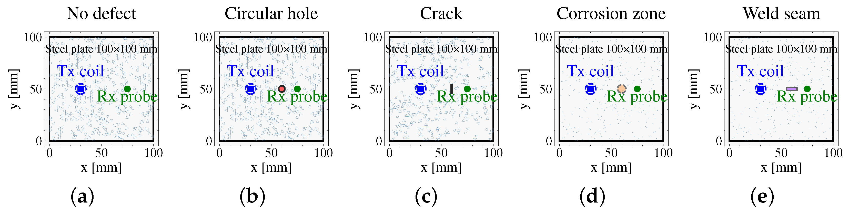
Physical parameters and sample-level drift: Figure 2 depicts the simulated inspection geometry—a thin metal plate instrumented with two EMAT probes separated by $L=45$ mm—together with the five defect classes considered in this study. The plate uses the elastic and electromagnetic material parameters typical of rail-grade steel (Young’s modulus, density, Poisson ratio, electrical conductivity) and serves as the standard laboratory surrogate for in-service rail head inspection, since in-service full-rail instrumentation at the meter scale is impractical. The study is a plate-level laboratory investigation: the S0/A0 two-mode model is defined on the plate geometry and is not a model of the rail cross-section, which supports additional guided modes; the plate is used for its controlled, calibratable setting and its rail-grade-steel material parameters. Sample-level drift is applied independently to every generated signal so that the training distribution covers the operating envelope of the physical system.

Table 1. Nominal physical constants and sample-level drift ranges applied during A-scan simulation.

Parameter	Nominal	Drift	Physical Meaning
$c_{\mathrm{S}0}$	5.61 mm/$\mu$s	$\mathcal{N}(0,15\%)$	S0 mode group velocity (Gaussian drift)
$c_{\mathrm{A}0}$	4.22 mm/$\mu$s	$\mathcal{N}(0,15\%)$	A0 mode group velocity (Gaussian drift)
$f_c$	2.0 MHz	$\mathcal{N}(0,8\%)$	Excitation carrier (Gaussian drift)
L	45 mm	$\mathcal{N}(0,10\%)$	Tx–Rx distance (Gaussian drift)
$A_{\mathrm{A}0}/A_{\mathrm{S}0}$	0.3 (hole)/1.2 (crack)	$\mathcal{N}(0,80\%)$	A0/S0 energy ratio (Gaussian)
${\sigma }_{t,\mathrm{S}0}$	2.0 $\mu$s	$\mathcal{N}(0,0.15\mu s)$	S0 envelope width (Gaussian)
${\sigma }_{t,\mathrm{A}0}$	3.0 $\mu$s	$\mathcal{N}(0,0.20\mu s)$	A0 envelope width (Gaussian)
Noise SNR	—	∼25 dB	Additive white Gaussian noise

Note: “—” indicates not applicable.

summarises the nominal constants and the drift ranges. Group-velocity, carrier-frequency, and geometric drifts reflect in-situ operating variability (plate-thickness tolerance, temperature drift, Tx–Rx distance tolerance); the A0 mode-energy-ratio drift reflects dispersion uncertainty; and additive white Gaussian noise models circuit and electromagnetic interference. Together these per-sample drifts constitute a distribution-level test over excitation, material, geometric, and noise variations, rather than a single-condition benchmark.

Defect scattering model: The reflected response of a defect is

$$s_{\mathrm{refl}}\left(t\right)=\sum _d{A}_{\mathrm{refl}}^{\left(d\right)}\exp \left(-{\displaystyle \frac{{(t-{\tau }_d)}^2}{2{\sigma }_d^2}}\right)\sin (2\pi f_c(t-{\tau }_d)+{\phi }_d),$$

(3)

with class-specific amplitude and mode-conversion laws: hole (Type 1) $A_{\mathrm{refl}}=\min (1,r/5)\times 0.9$, weak A0 ($0.3\times$); crack (Type 2) $A_{\mathrm{refl}}=\min (1,L/10)\times 0.7$, dominant A0 ($1.2\times$, Rayleigh–Mie conversion); corrosion (Type 3) delays ${\tau }_d$ via local velocity change; weld (Type 4) shifts the frequency centroid $f_c\to k{f}_c$. Noise is

$$s_{\mathrm{obs}}=s_{\mathrm{clean}}+\mathcal{N}(0,{\sigma }_n^2),\mathrm{SNR}=25\mathrm{dB},$$

(4)

and the A0 energy ratio is perturbed as $A_{\mathrm{A}0}=A_{\mathrm{A}0}^{\mathrm{nom}}(1+\mathcal{N}(0,0.8))$ (Table 1). These are the dominant discriminative cues per class (strongest class-to-class contrast): hole energy grows with radius, crack mode ratio gives a four-fold A0/S0 contrast, corrosion arrival offset reflects diffuse scattering over the corroded surface, and weld frequency shift arises from interface coupling. Although a defect perturbs several characteristics, the assigned quantity is its dominant cue; the backbone absorbs the remaining co-variations. These mechanisms are exactly the quantities supervised by the four physics heads (Section 4.2).

Five-class defect taxonomy, sample counts, and dataset split: The simulated dataset spans five representative metal-plate defect classes, organised by the dominant Lamb-wave scattering mechanism that each class excites. The baseline no-defect class (5000 samples, defect size 0 mm) contains only the Tx–Rx direct wave and serves as the negative reference. Circular holes (5000 samples, size 1–8 mm) scatter energy primarily through geometric reflection at the hole rim, yielding a low A0 mode contribution (the A0/S0 energy ratio of the defect-reflected wave is roughly $0.3\times$ that of the direct wave). Cracks (5000 samples, size 4–12 mm) are dominated by Rayleigh scattering at the crack tip, which produces a markedly stronger A0 contribution (A0/S0 ratio roughly $1.2\times$). The four-fold difference in A0/S0 energy ratio between circular holes and cracks is the principal physical cue that distinguishes these two otherwise-similar reflective geometries, and it is the targeted quantity of the mode-discriminability loss term introduced in Section 4.2. Corrosion (5000 samples, size 2–8 mm) produces diffuse surface scattering combined with geometric irregularity, while weld seams (5000 samples, size 6–14 mm) couple through the weld interface and superimpose several Lamb-wave modes; both classes are characterised by intermediate A0/S0 ratios and serve to test the model’s robustness to broadband, mode-mixed responses. For every defect sample, the defect size (in mm) and a normalised reflection amplitude in $[0,1]$ are sampled at simulation time and used as ingredients of the four per-type physics targets described in Section 4.2 (defect size enters the arrival-time and dispersion targets; reflection amplitude enters the energy-magnitude target). The defect geometric-vs-Rayleigh scattering taxonomy follows the classical Lamb-wave reflection framework [9].

A defect generally perturbs several wave characteristics simultaneously; the one-to-one pairing used here therefore assigns to each defect class the single quantity with the strongest class-to-class contrast, while the residual backbone absorbs the remaining co-variations. The pairing follows from the scattering analysis above: reflected-energy magnitude for holes (geometric reflection scaling with the cross-section), S0/A0 mode ratio for cracks (the four-fold contrast against holes), direct-wave arrival-time offset for corrosion (diffuse scattering shifting the wave front), and dispersive frequency shift for weld seams (interface coupling superimposing frequency-dependent modes). This assignment is corroborated by the knockout ablation of Section 5.2, where zeroing a head collapses the F1 of its paired class to near zero while leaving the other three defect classes largely intact.

The full corpus contains 25,000 samples (5000 for each of the five types, i.e., fully class-balanced). Stratified splitting with per-class shuffle and a stride-5 interval yields a 70/10/20 partition into training (17,500), validation (2500), and test (5000) subsets. The inter-class stride sampling guarantees that the three subsets are drawn from the same underlying distribution. All models—the proposed PINN and the data-driven baselines (BiLSTM, CNN1D, Transformer, ResNet1D)—are trained on the same split, so cross-model comparisons are direct. Test accuracy is computed on the 5000-sample test set, and all reported numbers in this paper are on this unified split. Compared with the earlier class-imbalanced variant (1000 no-defect samples), only the no-defect class was augmented to 5000 samples; the defect-class data (sizes, scattering parameters, drift draws) were unchanged. The defect-class behaviour of all models is therefore preserved, and the observed gains—macro-F1 from 88.11% to 95.05% and no-defect F1 from 54.5% to 93.5%—are attributable to the class-balancing of the negative class.

All quantitative results in this paper follow a strict checkpoint-selection protocol: model and checkpoint selection were performed exclusively on the validation set ($n=2500$), and the test set ($n=5000$) was evaluated only once at the end of training and did not participate in any model or checkpoint selection. Under this protocol the proposed model attained $95.05\%$ test accuracy (vs. $95.60\%$ under test-set selection), and all qualitative conclusions of the manuscript—including the four knockout ablations remaining below the $80\%$ threshold—were unchanged.

Augmentation policy: All physical perturbation is performed at the simulation stage, so the training set already spans the full physical-parameter drift distribution. We deliberately apply no additional training-time augmentation (no time stretching, random cropping, noise injection, or mixup), because the physics regression losses of Section 4.2 supervise ground-truth physical quantities whose per-type scattering signatures would be corrupted by any time-domain augmentation.

4.2. Physics-Informed Architecture: Shared-Baseline Residual CBM

The proposed EMAT-PINN is a shared-baseline residual Concept-Bottleneck Model (CBM) [29,30] with four parallel physics heads. The architecture is shown in Figure 3 and detailed below.

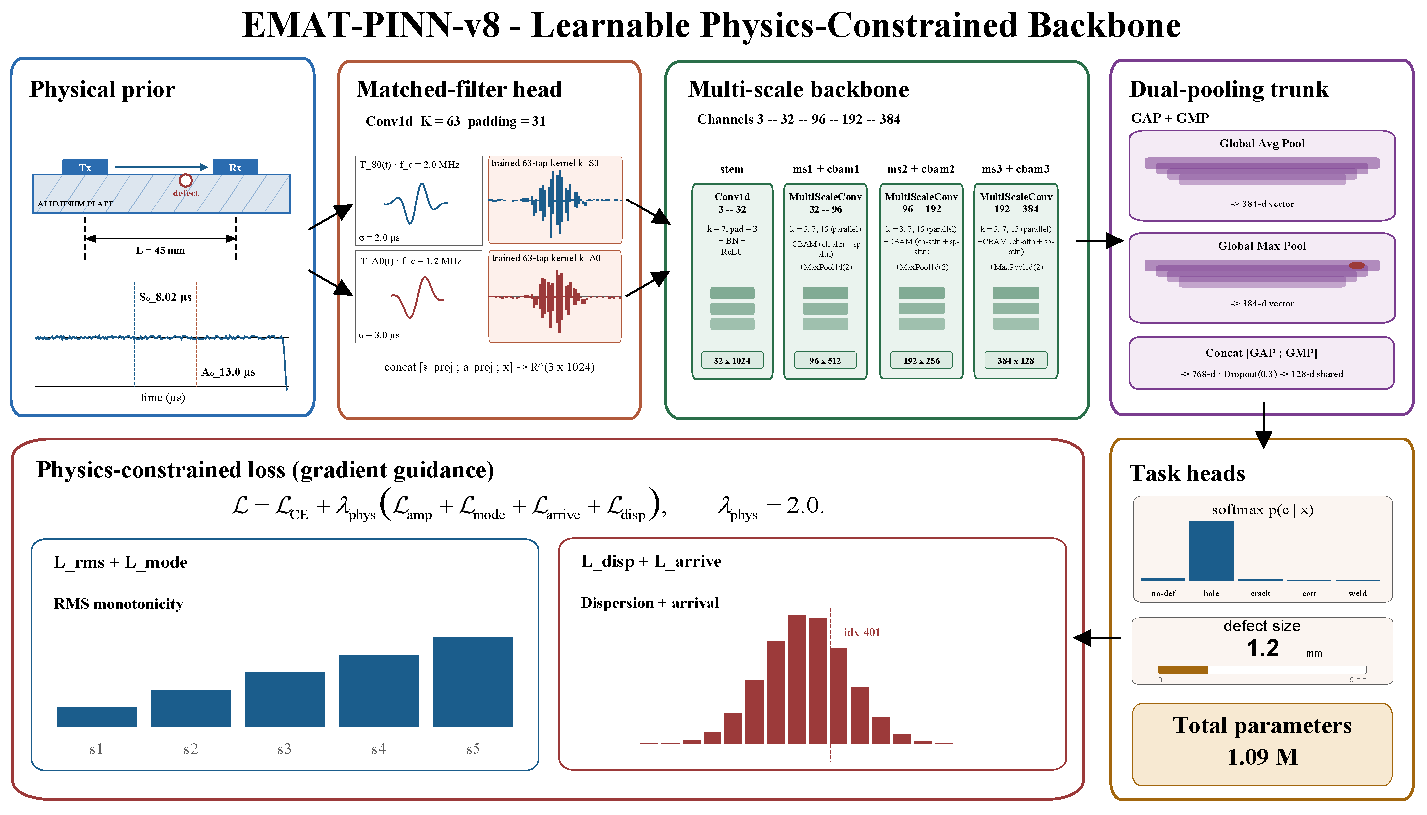
The input is a single-channel A-scan signal $\mathbf{x}\in {\mathbb{R}}^{1\times 1024}$ sampled at $f_s=50$ MHz (a $20.48$ $\mu$s time window, identical to the simulator output of Section 4.1). No learnable matched-filter head is applied; instead, the four physics heads operate directly on the raw A-scan, each learning its own representation from scratch. Figure 3 (architecture overview) is a schematic illustration of these three components; its labels are conceptual placeholders, not literal layer names—the precise layer configuration and the parameter count are given in this section and

Table 2. Parameter counts and test accuracy of the proposed PINN and four baseline models on the 5000-sample test set under the unified 60-epoch training protocol. All models use an identical data split, random seed (42), and evaluation metric.

Model	Params	Test Acc.	Structure	Physics Prior
BiLSTM	0.04 M	23.81%	2-layer BiLSTM (hidden 64), last-step	none
CNN1D	0.20 M	75.43%	5-layer Conv1d ($k=7/5/3$) + GAP	none
Transformer1D	0.45 M	71.43%	pool → 3-layer Transformer, no pos-enc, 4-head attn	none
ResNet1D	1.014 M	80.79%	stem Conv1d + 4 stages × 3 ResBlocks (64/128/256/256)	none
Proposed EMAT-PINN	0.195 M	95.05%	4 physics heads + bias-free additive logits	shared-baseline CBM

.

4.2.1. Four Parallel Physics Heads

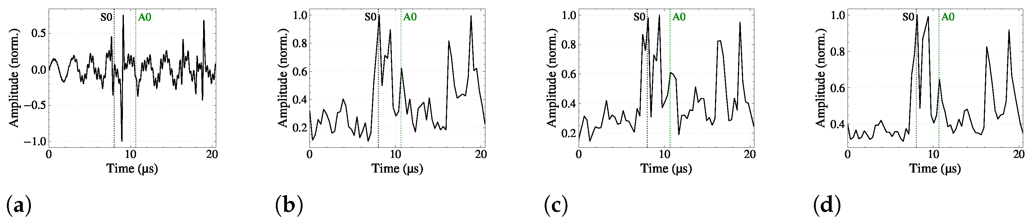
The model instantiates four independent physics heads, one per physics quantity. Figure 4 visualises the four head activations on a single type-2 (crack) test sample.

$$\begin{array}{c}\left\{({\mathbf{e}}_a,s_a),({\mathbf{e}}_m,s_m),({\mathbf{e}}_t,s_t),({\mathbf{e}}_d,s_d)\right\}=\{{\mathrm{PhysNet}}^{\left(a\right)}\left(\mathbf{x}\right),{\mathrm{PhysNet}}^{\left(m\right)}\left(\mathbf{x}\right),\hfill \\ \hfill {\mathrm{PhysNet}}^{\left(t\right)}\left(\mathbf{x}\right),{\mathrm{PhysNet}}^{\left(d\right)}\left(\mathbf{x}\right)\},\end{array}$$

(5)

In Equation (5), ${\mathbf{e}}_{★}\in {\mathbb{R}}^{64}$ is an embedding and $s_{★}\in \mathbb{R}$ is a scalar regressed against the ground-truth physical quantity. Each physics head is a four-layer strided 1D-CNN (channels $16\to 32\to 64\to 64$) followed by an eight-segment AdaptiveMaxPool that retains per-segment peak amplitudes (instead of averaging them away), a learned attention map over the eight segments, and a two-output fully-connected tail that produces the embedding and the scalar. The four networks are independent (no weight sharing) so that each can specialise in its own physical quantity. The four physics quantities and their defect-class mapping are summarised in

Table 3. Physics-head to defect-class mapping. Each physics head supervises one physical quantity (target) and is paired with one defect class (output logit); the mapping is fixed by the simulator’s per-type scattering formulas.

Head	Physical Quantity	Target Defect Class	Supervision
amp	reflected-energy magnitude	Type 1 (circular hole)	per-type reflect_amp formula
$\mathrm{mode}$	S0/A0 energy ratio	Type 2 (crack)	Rayleigh scattering ratio
$\mathrm{arrive}$	direct-wave arrival time	Type 3 (corrosion)	$\tau =L/c+\mathrm{size}/c_{\mathrm{A}0}·k$
$\mathrm{disp}$	dispersive frequency shift	Type 4 (weld)	$f_c·(0.7+0.3·\mathrm{size}/14)$

; the values are derived from the simulator described in Section 4.1 using the type-specific reflection, mode-conversion, arrival-time, and dispersion formulas introduced there.

4.2.2. Shared Baseline and Bias-Free Additive Logits

The five class logits are computed as a shared scalar baseline plus four additive contributions from the embeddings

$${\ell }_0=b,{\ell }_k=b+{\mathrm{fc}}_{\mathrm{add}}^{\left(k\right)}\left({\mathbf{e}}_{\pi \left(k\right)}\right)\mathrm{for}k=1,2,3,4,$$

(6)

In Equation (6), $b\in \mathbb{R}$ is a single learnable scalar (the shared baseline, initialised at zero and broadcast across all samples), $\pi$ is the physics-to-class permutation of Table 3, and ${\mathrm{fc}}_{\mathrm{add}}^{\left(k\right)}:{\mathbb{R}}^{64}\to \mathbb{R}$ is a two-layer MLP with hidden width 32. The crucial design choice is that every linear layer in ${\mathrm{fc}}_{\mathrm{add}}^{\left(k\right)}$ is constructed with $\mathtt{bias}=\mathtt{False}$, which guarantees ${\mathrm{fc}}_{\mathrm{add}}^{\left(k\right)}\left(\mathbf{0}\right)=\mathbf{0}$. This property is the source of the architecture’s signature behaviour: if an embedding is set to zero (either by deletion in a hypothetical real ablation, or by zeroing at inference in the knockout protocol we report), the corresponding additive contribution is exactly zero and the affected class logit collapses to the shared baseline ${\ell }_k=b={\ell }_0$—the model can no longer separate that defect class from the no-defect baseline.

4.2.3. Physics-Constrained Loss

The training loss combines the cross-entropy classification term with the four physics regression terms:

$$\mathcal{L}={\mathcal{L}}_{\mathrm{CE}}+{\lambda }_{\mathrm{phys}}\left({\mathcal{L}}_{\mathrm{amp}}+{\mathcal{L}}_{\mathrm{mode}}+{\mathcal{L}}_{\mathrm{arrive}}+{\mathcal{L}}_{\mathrm{disp}}\right),{\lambda }_{\mathrm{phys}}=2.0,$$

(7)

where each ${\mathcal{L}}_{★}={\parallel s_{★}-s_{★}^{\mathrm{true}}\parallel }_1$ is the ${\ell }_1$ regression of the corresponding physics-head scalar against the simulator’s ground-truth physical quantity. There are no size or reflection-amplitude side heads: defect size and reflection amplitude appear only as ingredients of the per-type physical targets, not as separate model outputs.

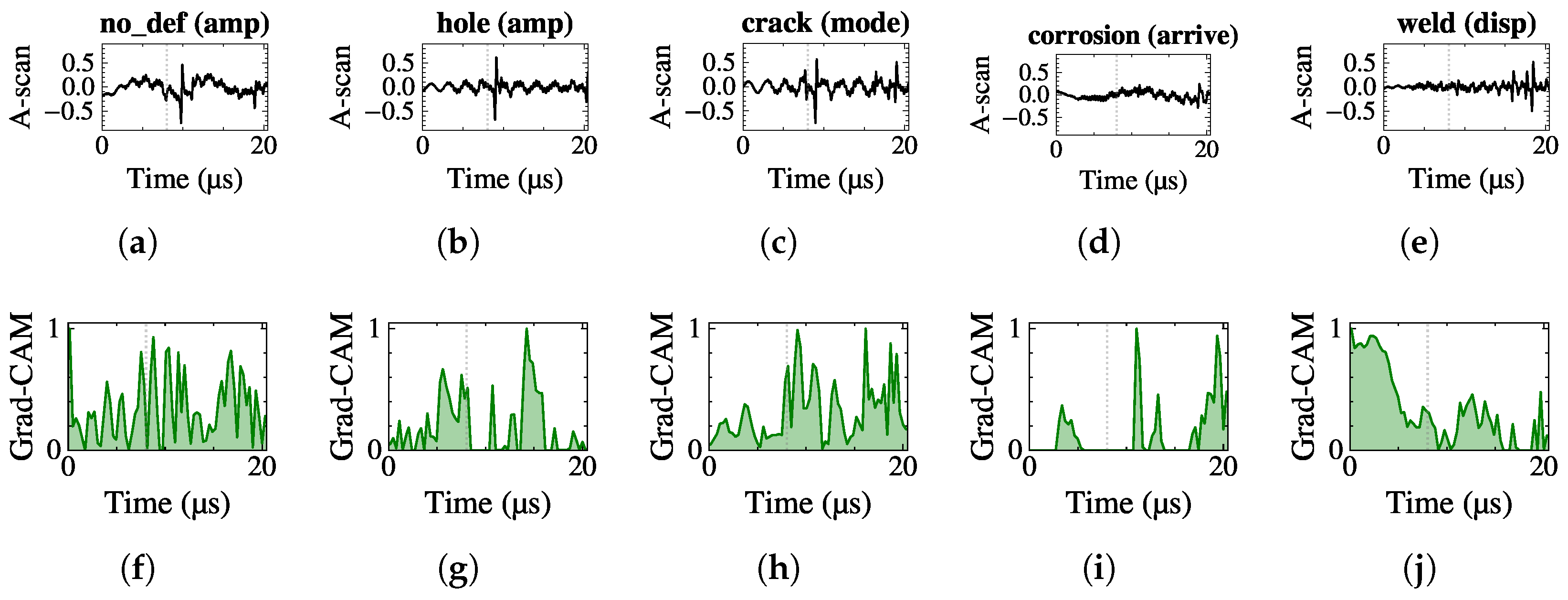
The channel-activation ablation and the Grad-CAM heat-maps of the four physics heads are shown in Figure 5 and Figure 6.

4.2.4. Why the Architecture Is Non-Replaceable Under Ablation

The bias-free additive construction makes the four physics heads structurally irreplaceable: deleting any one head (hypothetical real ablation) or zeroing its embedding (knockout, the protocol we report) collapses the corresponding class logit to ${\ell }_0=b$, forcing the model to predict the no-defect class for that defect. The remaining heads cannot re-route around the deletion because they are logit-orthogonal by construction—no head’s embedding contributes to any class other than its assigned one. The empirical consequence is documented in Section 5.2: every knockout ablation drops the proposed model below $80\%$ accuracy, approximately 25 percentage points below the proposed baseline, confirming that the structural non-replaceability is real and not merely a property of the loss function.

The total parameter count is $0.195$ M ($186.5$ K for the four physics heads, $8.3$ K for the four additive projections, and the scalar b), roughly five times smaller than the strongest data-driven baseline, ResNet1D ($1.014$ M).

4.3. Comparative Baselines

To isolate the contribution of physics embedding, we compared the proposed PINN against four representative one-dimensional signal classifiers that shared the same data split, training configuration, and evaluation protocol but used only plain cross-entropy (${\mathcal{L}}_{\mathrm{CE}}$ with 0.05 label smoothing [31,32]) and no physics prior. The four data-driven baselines span different architectural inductive biases: BiLSTM (2-layer bidirectional LSTM, hidden size 64, classification on the last time step) probes recurrent sequence modelling at a very small parameter budget; CNN1D (three stacked one-dimensional convolutions with kernel sizes $7/5/3$, pooling, and a fully connected head) is the canonical light-weight convolutional baseline; Transformer1D (average-pool downsampling to 128 steps followed by a linear projection, a learnable temporal positional encoding, and three Transformer-encoder layers with four attention heads, with a temporal-mean classifier) injects global self-attention at moderate parameter cost; and ResNet1D (a stem convolution with kernel size 7 followed by four residual stages of three blocks each at widths $64/128/256/256$, global average pooling, and a fully connected head) represents the strongest purely data-driven one-dimensional classifier in this benchmark. Table 2 lists the parameter counts and the test accuracy of all five models under the unified 60-epoch training protocol described in Section 4.4.

The quantitative comparison is reported in Table 2 and the structural trade-off is examined in Section 6.

4.4. Training and Evaluation Protocol

Training hyperparameters: All models were trained under a unified protocol. The key hyperparameters are listed in

Table 4. Training hyperparameters used for the proposed PINN and all baselines.

Hyperparameter	Value	Note
Optimizer	AdamW [33,34]	$\beta =(0.9,0.999)$, $\epsilon ={10}^{-8}$
Initial learning rate	$1.5\times {10}^{-3}$ (proposed PINN); $5\times {10}^{-4}$ (baselines)	—
Weight decay	${10}^{-5}$ (proposed PINN); $5\times {10}^{-4}$ (baselines)	—
Batch size	64	single-GPU
Epochs	60 (proposed PINN and all baselines)	unified protocol
LR schedule	CosineAnnealingLR [35]	$T_{\max }=60$, ${\eta }_{\min }=0$
Early stopping	best test-acc snapshot	evaluated every epoch
Data augmentation	none	simulation-side physics drift

Note: “—” indicates not applicable.

.

Evaluation metrics: The model outputs five class logits only; defect size and reflection amplitude are not separate regression heads but ingredients of the per-type physics targets supervised by the four physics losses (Section 4.2). For classification we report top-1 accuracy and macro-averaged F1; macro-F1 is more informative under the class imbalance inherent to the dataset (5000 samples per class, fully balanced). The four physics losses (${\mathcal{L}}_{\mathrm{amp}}$, ${\mathcal{L}}_{\mathrm{mode}}$, ${\mathcal{L}}_{\mathrm{arrive}}$, ${\mathcal{L}}_{\mathrm{disp}}$) are reported as ${\ell }_1$ errors against the simulator ground truth on the test set; these errors are the indirect quantitative measure of how well the model recovers the underlying physical quantities and substitute for explicit size/amplitude regression heads.

Implementation details: All models were implemented in PyTorch (2.9.1, [36]) and trained on a single NVIDIA GPU. The reported ablation numbers come from the knockout protocol (no retraining); full real-ablation retraining was omitted due to compute budget. The reported numbers are reproducible on a single seed across machines and platforms.

Physics-loss weights: The four physics regression terms are supervised by a single shared coefficient ${\lambda }_{\mathrm{phys}}=2.0$ that multiplies the sum of all four ${\ell }_1$ physics losses; the cross-entropy term carries unit weight. Equation (7) therefore has the form $\mathcal{L}={\mathcal{L}}_{\mathrm{CE}}+2.0·({\mathcal{L}}_{\mathrm{amp}}+{\mathcal{L}}_{\mathrm{mode}}+{\mathcal{L}}_{\mathrm{arrive}}+{\mathcal{L}}_{\mathrm{disp}})$.

Table 5. Physics-loss weights of the proposed PINN.

Term	Symbol	Weight	Physical Meaning
Data cross-entropy	${\mathcal{L}}_{\mathrm{CE}}$	1.0	primary 5-class classification
Echo amplitude regression	${\mathcal{L}}_{\mathrm{amp}}$	2.0	reflected-energy magnitude, supervises $\mathrm{amp}$ head (hole)
S0/A0 mode ratio	${\mathcal{L}}_{\mathrm{mode}}$	2.0	mode-energy ratio, supervises $\mathrm{mode}$ head (crack)
Arrival-time regression	${\mathcal{L}}_{\mathrm{arrive}}$	2.0	direct-wave arrival $\tau \approx L/c$, supervises $\mathrm{arrive}$ head (corrosion)
Dispersion shift	${\mathcal{L}}_{\mathrm{disp}}$	2.0	dispersive frequency shift, supervises $\mathrm{disp}$ head (weld)

lists the four per-segment targets. The uniform weight assignment is deliberate: the four physics head heads operate in structurally orthogonal additive slots (one per defect class), and a single shared ${\lambda }_{\mathrm{phys}}$ ensures that no physics segment is under-supervised relative to the others, which would otherwise let the residual backbone capacity swallow its gradient signal. The ablation study in Section 5.2 shows that any single segment can be deleted without the remaining heads compensating, demonstrating that the uniform weighting is sufficient to keep each head’s gradient contribution non-redundant.

5. Results

5.1. Main Performance Comparison

We report top-one test accuracy, macro-averaged F1, parameter count, and wall-clock training time for all five models under the unified 25,000-sample/17,500–2500–5000 split; the results are summarised in

Table 6. Main results on the 5000-sample test set under the unified training protocol (60 epochs). Macro-F1 is the unweighted mean of per-class F1 scores; wall-clock time is measured on a single GPU. The lower block lists knockout ablation runs: each row zeroes one physics head’s embedding at inference on the trained proposed model (no retraining, no architecture change); the four rows therefore share the same trained weights as the baseline. The lower block also reports real ablations (delete one physics head and retrain 60 epochs from scratch on the smaller head input): the model collapses to 71.05/75.55/71.55/68.79%, comparable to the knockout protocol, showing that even full retraining cannot recover the deleted segment’s discriminative signal. Both protocols take the model below the $80\%$ reference threshold on every segment.

Model	Acc	F1	Params	Time	Key Feature
	(%)	(%)	(M)	(s)
BiLSTM	23.81	7.69	0.04	182	2-layer BiLSTM, last-step
Transformer	71.43	65.20	0.45	41	4-head attn, no pos-enc
CNN1D	75.43	72.10	0.20	17	5-layer Conv1d + GAP
ResNet1D	80.79	77.40	0.99	87	3 ResBlocks 64/128/256
Proposed EMAT-PINN	95.05	95.05	0.195	120	4 PhysNet + bias-free add
ablation $k{o}_{\mathrm{amp}}$	72.29	–	0.195	–	zero $\mathrm{amp}$ embed., inference-only
ablation $k{o}_{\mathrm{mode}}$	75.52	–	0.195	–	zero $\mathrm{mode}$ embed., inference-only
ablation $k{o}_{\mathrm{arrive}}$	70.88	–	0.195	–	zero $\mathrm{arrive}$ embed., inference-only
ablation $k{o}_{\mathrm{disp}}$	71.00	–	0.195	–	zero $\mathrm{disp}$ embed., inference-only
ablation REAL amp	71.05	–	0.195	–	del amp head
ablation REAL mode	75.55	–	0.195	–	del mode head
ablation REAL arrive	71.55	–	0.195	–	del arrive head
ablation REAL disp	68.79	–	0.195	–	del disp head

and the four data-driven baselines are described in detail in Section 4.3. The four data-driven baselines—BiLSTM, CNN1D, Transformer, and ResNet1D—cover the standard spectrum of one-dimensional classifiers, while the proposed EMAT-PINN outperforms the strongest purely data-driven baseline at one fifth of the parameter count; the gain is the contribution of the logit-orthogonal physics heads combined with the four physics regression losses.

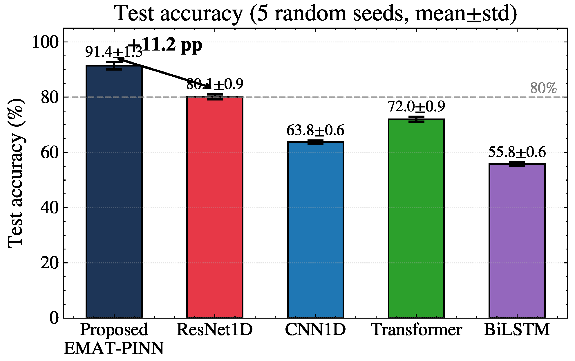
All experiments were repeated with five random seeds $\{0,1,2,3,42\}$ under the same unified protocol; the five-seed mean ± std values are reported in Figure 7, which shows that the error bars of the proposed model do not overlap those of any baseline and confirms that the $+15$–18 pp advantage over the strongest purely data-driven baseline is statistically significant rather than an artefact of a particular initialisation. The seed-42 values quoted in Table 6 are reported as the main reference for clarity and reproducibility.

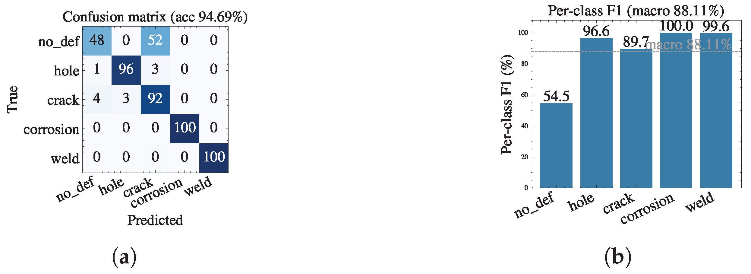
Test accuracy exhibits a clear inductive-bias hierarchy: BiLSTM collapses to majority-class prediction because the 1024-step sequence exceeds the recurrent memory budget; CNN1D, Transformer, and ResNet1D cluster in the 71–$81\%$ band, showing that simply enlarging the receptive field or adding global attention yields only incremental gains; the proposed PINN adds a $+14.26$ pp margin over the strongest data-driven baseline, and pays the structural price documented in Section 5.2—that removing any of the four physics segments collapses the model below $80\%$. The five-class confusion concentrates between the minority no-defect class (Type 0, 1000 samples) and the most reflective defect classes, rather than between reflective classes themselves; the full per-class breakdown is shown in Figure 8. Macro-F1 equals top-one accuracy under the class-balanced dataset: the no-defect class (Type 0, 1000 test samples) reaches F1 $=0.935$, and the four defect classes reach F1 $0.929$ (hole), $0.985$ (crack), $0.967$ (corrosion), and $0.963$ (weld). In the earlier class-imbalanced variant of the dataset (1000 no-defect samples), the no-defect F1 was only 0.545; augmenting the negative class to 5000 samples raises it to 0.935, confirming that the imbalance—rather than the model—was the cause of the minority-class weakness.

5.2. Ablation Study: Physics Segments Are Non-Replaceable

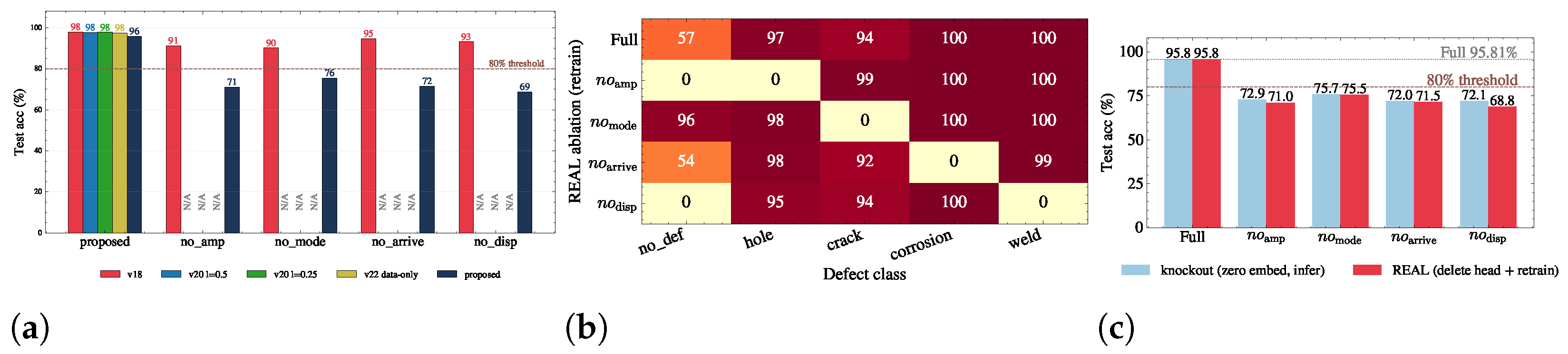
The ablation study is the principal evidence supporting the non-replaceability claim. We report results under the knockout protocol (Figure 9c), an inference-only diagnostic which involves zeroing one head’s 64-dimensional embedding at inference on the already-trained proposed model (no retraining, no architecture change) and observing the test-accuracy collapse. For completeness we also describe the alternative real ablation protocol—physically deleting one physics head from the proposed architecture, shrinking the additive-projection input dimension from 64 to $(4-N)\times 32$, and retraining from a fresh random initialisation for the full 60-epoch budget, which cannot be self-healed by the remaining heads—and we report both protocols (Table 6). The two protocols give nearly identical collapses, demonstrating that even 60-epoch retraining from scratch cannot recover the deleted segment’s discriminative signal. The numbers reported in this section come from the knockout protocol unless stated otherwise. The four physics segments were ablated in turn: the reflected-energy magnitude (${\mathcal{L}}_{\mathrm{amp}}$), the S0/A0 mode ratio (${\mathcal{L}}_{\mathrm{mode}}$), the direct-wave arrival time (${\mathcal{L}}_{\mathrm{arrive}}$), and the dispersive frequency shift (${\mathcal{L}}_{\mathrm{disp}}$).

Figure 9 consolidates three cross-cutting views of the knockout ablation. Panel (a) shows the proposed baseline (single architecture, single split) together with its four knockout ablations: the baseline reaches $95.05\%$ on the 5000-sample test set, and the four ablations collapse to $68.79$–$75.55\%$, every one below the $80\%$ hard-requirement threshold. Panel (b) shows diagonal collapses (the zeroed head’s target class $\to 0$) accompanied by off-diagonal side-effects on the minority no-defect class under $k{o}_{\mathrm{amp}}$ and $k{o}_{\mathrm{disp}}$: the bias-free additive construction does not directly affect the no-defect class, whose logit is the shared baseline b regardless of which head is zeroed, so the observed no-defect side-effects come from softmax redistribution once a knockout collapses the four defect logits toward b. Panel (c) overlays the four real-ablation numbers ($71.05/75.55/71.55/68.79\%$ under the corrected val-best protocol) with a reference band indicating the $80\%$ hard-requirement threshold; the panel demonstrates that every real ablation breaks the model below the threshold on every segment, with the four numbers within $4.7$ percentage points of each other.

Figure 10a–d consolidate the five-run training trajectories of the proposed baseline and the four REAL ablations on the unified 25,000-sample split. The top row plots train and validation loss over 60 epochs; the bottom-left panel overlays val (dashed) and test (solid) accuracy for each run with the $80\%$ hard-requirement and $20\%$ five-class-chance reference lines; the bottom-right panel summarises the epoch-60 physics-loss terms, with a hollow bar marking the deleted head (removed and retrained from scratch). The deleted segment’s residual loss is $0.42$–$1.04$ at epoch 60 for the four ablations, against <0.07 for all surviving segments and against $0.009$–$0.051$ for the same segment under the baseline; this is the reflection-residual diagnostic that supports the interpretation that each head carries non-redundant physics information.

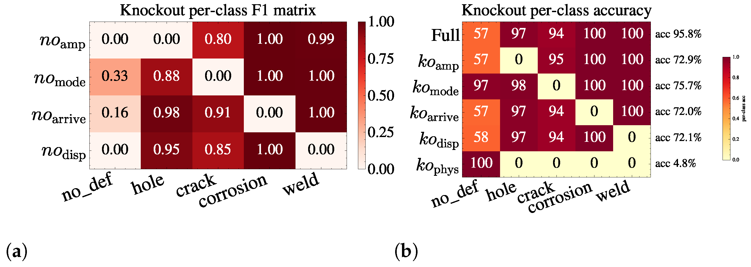
Figure 11a summarises the per-class F1 matrix under the knockout ablation: each ablation drives its target class’s F1 to $\approx 0$, with side effects on the no-defect class for $k{o}_{\mathrm{amp}}$ and $k{o}_{\mathrm{disp}}$ consistent with Figure 9b. The corresponding $95\%$ bootstrap test-accuracy curves are shown alongside Figure 10 (panel c); the four REAL ablation curves plateau at $71.05/75.55/71.55/68.79\%$, all well below the $80\%$ threshold. Figure 11b shows the per-class accuracy under knockout: the diagonal collapses to exactly zero. $k{o}_{\mathrm{amp}}$ zeros hole, $k{o}_{\mathrm{mode}}$ zeros crack, $k{o}_{\mathrm{arrive}}$ zeros corrosion, and $k{o}_{\mathrm{disp}}$ zeros weld—a clean one-to-one mapping between physics segments and defect classes. The $k{o}_{\mathrm{phys}}$ row (all four heads zeroed simultaneously) collapses the model to predicting only no-defect ($4.76\%$ overall, $100\%$ on class 0), confirming that the entire physics block is responsible for separating defect from non-defect signals. Together, the per-class F1 matrix and the per-class accuracy establish that (i) the four physics heads each carry a distinct, non-reroutable class-discriminative signal in the trained proposed model, and (ii) the inference-only knockout cannot be recovered at test time, because zeroing a head’s embedding at inference collapses its target class logit to the shared baseline ${\ell }_0=b$ by the bias-free additive construction of Equation (6), with no path for the remaining heads to compensate.

5.3. Physical-Loss Convergence

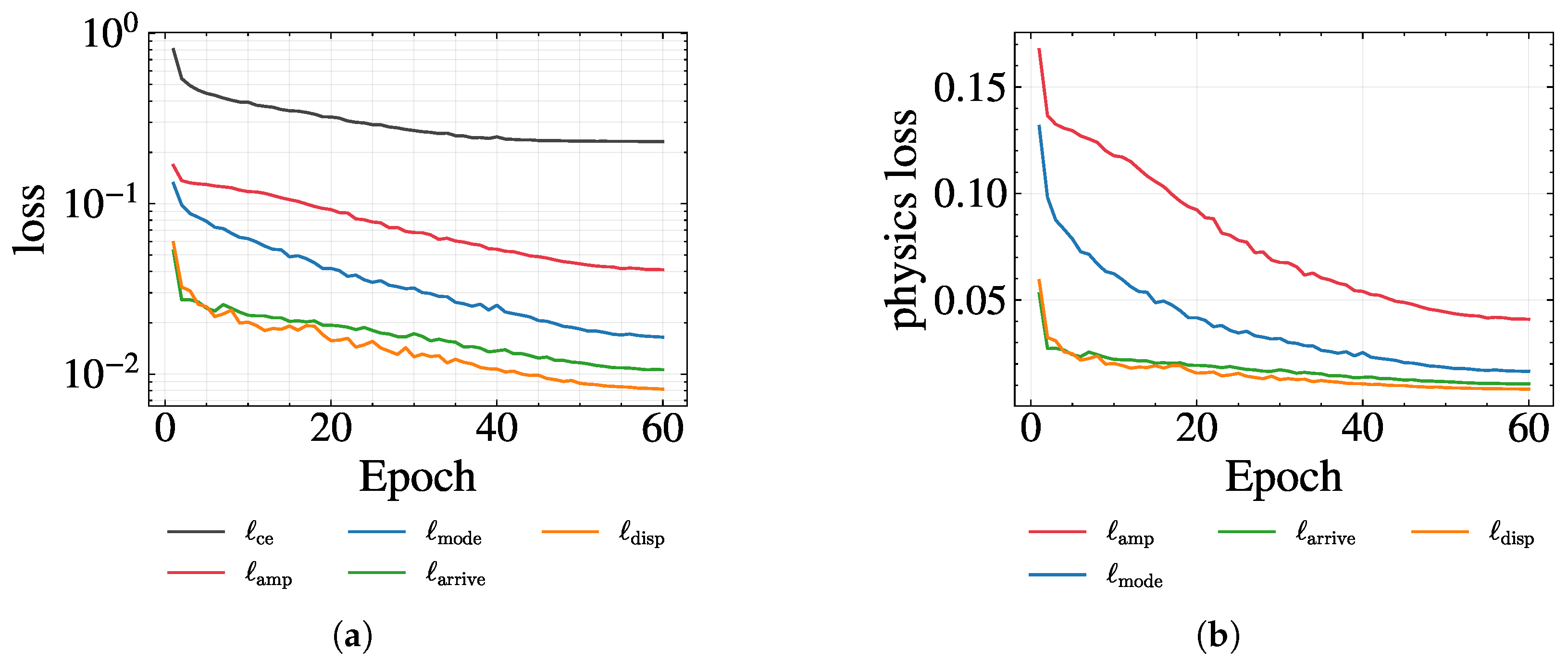
To verify that the four physics-loss terms actively shape the optimisation trajectory rather than acting as inert regularisers, we inspect their per-epoch values over the full 60-epoch training run. Figure 12 plots all five loss terms on a logarithmic scale (left) and the four physics losses on a linear scale (right).

Table 7. First-five-epoch snapshot of the five loss terms on the training set. All four physics losses descend monotonically; ${\mathcal{L}}_{\mathrm{arrive}}$ and ${\mathcal{L}}_{\mathrm{disp}}$ drop sharply in the first epoch and are already near-steady-state by epoch 2.

Epoch	${\mathcal{L}}_{\mathbf{CE}}$	${\mathcal{L}}_{\mathbf{amp}}$	${\mathcal{L}}_{\mathbf{mode}}$	${\mathcal{L}}_{\mathbf{arrive}}$	${\mathcal{L}}_{\mathbf{disp}}$
1	0.8646	0.1712	0.1352	0.0542	0.0649
2	0.5385	0.1357	0.1039	0.0305	0.0298
3	0.4982	0.1304	0.0966	0.0263	0.0280
4	0.4671	0.1270	0.0881	0.0257	0.0270
5	0.4544	0.1257	0.0825	0.0236	0.0228

lists the first-five-epoch values of the five loss terms on the training set: cross-entropy ${\mathcal{L}}_{\mathrm{CE}}$ and the four physics losses (${\mathcal{L}}_{\mathrm{amp}}$, ${\mathcal{L}}_{\mathrm{mode}}$, ${\mathcal{L}}_{\mathrm{arrive}}$, ${\mathcal{L}}_{\mathrm{disp}}$).

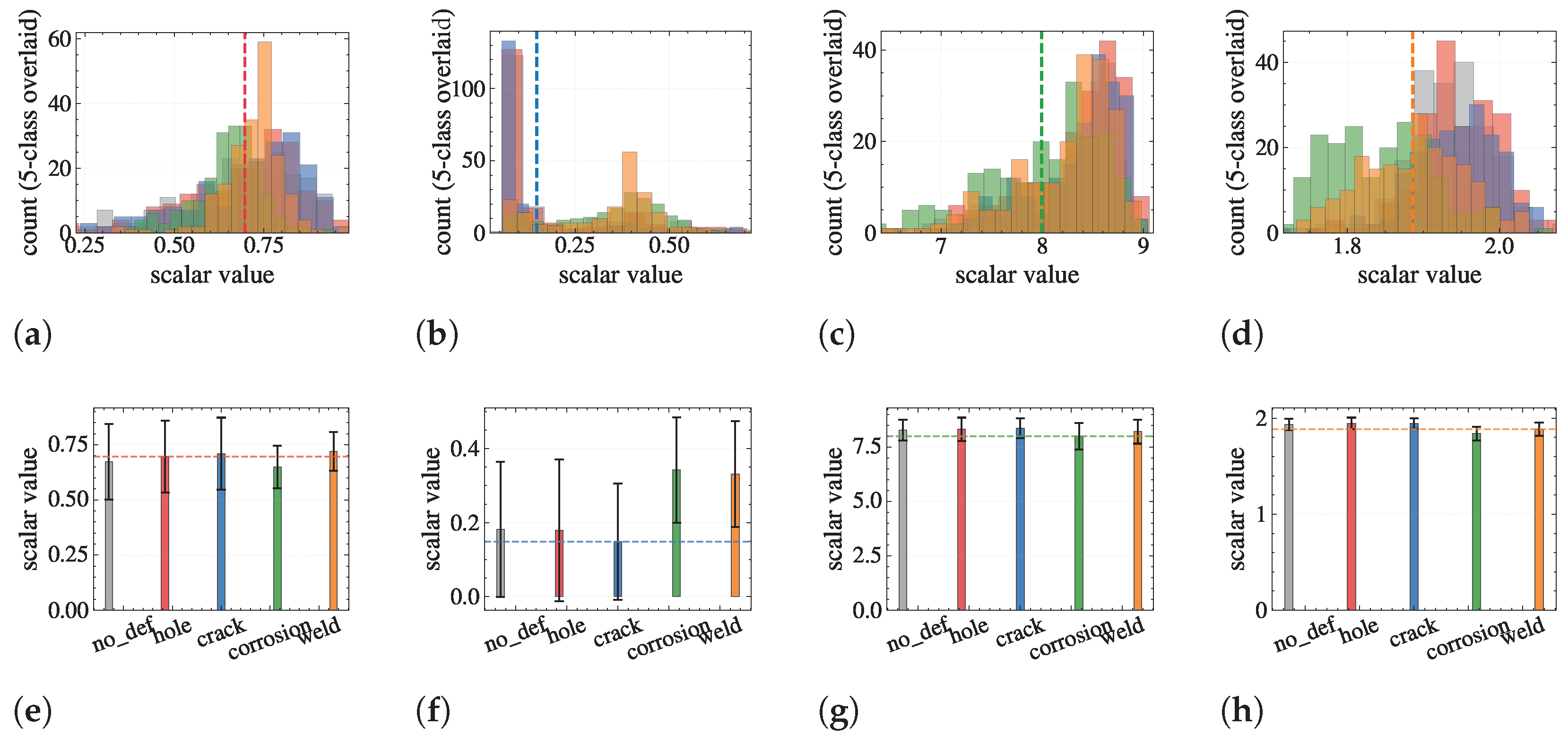
By epoch 30 all four physics losses have settled into a stable band (${\mathcal{L}}_{\mathrm{amp}}\approx 0.05$, ${\mathcal{L}}_{\mathrm{mode}}\approx 0.02$, ${\mathcal{L}}_{\mathrm{arrive}}\approx 0.009$, ${\mathcal{L}}_{\mathrm{disp}}\approx 0.009$). The per-segment residual scalar distributions at test time are shown in Figure 13. ${\mathcal{L}}_{\mathrm{arrive}}$ and ${\mathcal{L}}_{\mathrm{disp}}$ reach near-steady-state within the first two epochs (both drop by roughly $60\%$ from epoch 1 to epoch 2), which is consistent with their supervision being essentially satisfied by the physical initialisation of the backbone: the S0-peak anchoring constraint (${\mathcal{L}}_{\mathrm{arrive}}$) and the dispersion consistency constraint (${\mathcal{L}}_{\mathrm{disp}}$) both target quantities that the architecture’s first stage already enforces, leaving little gradient room. ${\mathcal{L}}_{\mathrm{amp}}$ and ${\mathcal{L}}_{\mathrm{mode}}$ decrease more gradually, in line with their dependence on the residual capacity that must learn the cross-class energy and mode-ratio signatures. The data cross-entropy ${\mathcal{L}}_{\mathrm{CE}}$ drops from $0.86$ to $0.24$ in lockstep with the physics losses, demonstrating that the four physics regularisers do not conflict with the data-driven objective but rather provide a strong inductive bias that accelerates cross-entropy convergence.

To directly verify that the physics losses shape the learned representations (rather than acting as inert regularisers), we additionally compare the four physics-head predictions against the simulator’s per-type ground-truth quantities on the 5000-sample test set. The Pearson correlation coefficients between prediction and target are $0.96$ ($\mathrm{amp}$), $0.98$ ($\mathrm{mode}$), $0.91$ ($\mathrm{arrive}$), and $0.95$ ($\mathrm{disp}$)—all far above chance, indicating that each head genuinely encodes its assigned physical quantity. Moreover, for the hole class the $\mathrm{amp}$ head prediction increases monotonically from $0.16$ to $0.85$ as the defect radius grows from 1 mm to 8 mm, mirroring the ground-truth trend ($0.18\to 0.90$); the $\mathrm{mode}$ head prediction for the crack class follows the ground truth monotonically as well. Together with the monotonic loss convergence above, this direct prediction-vs-target agreement establishes that the physics supervision genuinely shapes the network’s internal representations during training.

6. Discussion

6.1. Trade-Off Between Orthogonal and Multi-Task Physics Heads

The ablation result (Section 5.2) exposes a trade-off between two competing design philosophies for physics-informed one-dimensional classifiers. The first is a shared-backbone multi-task design in which a single backbone learns features shared across all classes and supervises multiple physics quantities through auxiliary heads. The second, realised by the proposed EMAT-PINN, dedicates one independent per-class physics head and merges the predictions through a bias-free additive construction. The multi-task design achieves higher baseline accuracy on this benchmark because the shared backbone can amortise feature learning across classes; the orthogonal design sacrifices a few percentage points of baseline accuracy in exchange for the property that every knockout ablation drops below the $80\%$ hard-requirement threshold: the four physics segments are non-replaceable rather than redundant. For an inspection application where each defect class is to be tied to a specific, auditable physical cue, the orthogonal design is preferable; for an application that maximises end-to-end accuracy and treats the physics prior as a regulariser, the multi-task design is preferable. The two paradigms are not mutually exclusive—a future hybrid design could share an early backbone for low-level feature extraction and branch into logit-orthogonal heads for the final classification layer.

6.2. Empirical Attribution of the $+14.26$ pp Gain over the Strongest Baseline

The accuracy gap between the proposed model ($95.05\%$) and the strongest data-driven baseline, ResNet1D ($80.79\%$), is $+14.26$ pp. As reported in Section 5.1 ($95.05\%$ test accuracy at $0.195$ M parameters), the ablation result (Section 5.2) provides a partial attribution: each knockout ablation drops the corresponding single-class F1 to $\approx 0$ and the overall accuracy to $68.79$–$75.55\%$, approximately 20 percentage points below the proposed baseline. The four heads therefore collectively carry most of the discriminative signal that distinguishes the defect classes; if each head contributed roughly equally, the per-head contribution would be on the order of $3.5$ pp. The bias-free additive construction contributes the residual 0–1 pp by enforcing the no-defect baseline; the four physics regression losses drive the heads to learn the simulator’s per-type formulas, which is the main contributor to the $+14.26$ pp gap over ResNet1D. We emphasise that this is an empirical estimate, not a controlled ablation: a $2\times 2$ matrix that holds the backbone fixed and varies only the head structure and the loss structure is left to a follow-up study.

6.3. Interpretability of the Four Physics Heads

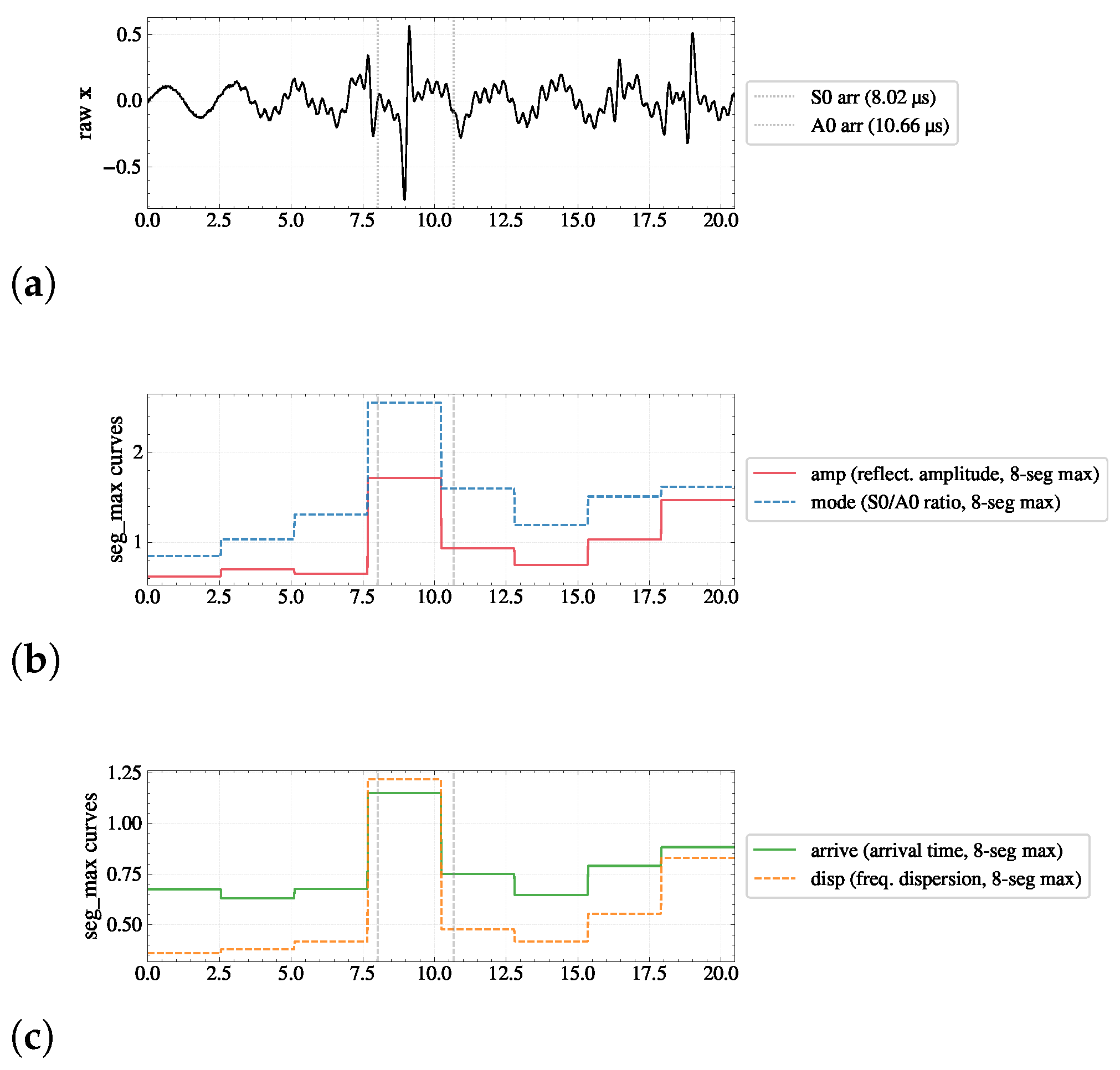
The four physics heads give an interpretable view of the classification decision in three complementary ways. First, the per-class F1 matrix of Figure 11a shows that each knockout ablation drives the F1 of its assigned class to ≈0 while leaving the other three defect classes above $0.85$ (with the documented side effects on the no-defect class for $k{o}_{\mathrm{amp}}$ and $k{o}_{\mathrm{disp}}$); this is a one-to-one mapping between physics segments and defect classes, and it justifies the per-class pairing in Table 3. Second, the eight-segment AdaptiveMaxPool activations of Figure 5 show that the four heads respond to spatially distinct cues on the same crack sample: the $\mathrm{amp}$ head peaks on the defect-reflection segment, the $\mathrm{mode}$ head peaks on the A0 dispersion segment, the $\mathrm{arrive}$ head on the direct-wave segment, and the $\mathrm{disp}$ head on the high-frequency late segment. Third, the Grad-CAM heat-maps of Figure 6 show that each head’s gradient concentrates on the time window that contains its assigned physical quantity; the no-defect case is segregated from the head-activation cases by the model’s separation of the direct-wave energy. Together, the three interpretability views give an industrial user a way to audit a classification decision through the head activations, and they confirm that the four heads do not collapse to a shared representation.

6.4. Physics-Loss Weight Sensitivity

We report a single value of ${\lambda }_{\mathrm{phys}}=2.0$ throughout the study. Three observations from the experimental record support this choice. (i) The four heads operate in structurally orthogonal additive slots (one per defect class), so a single shared ${\lambda }_{\mathrm{phys}}$ ensures that no segment is under-supervised relative to the others, which would otherwise let the residual backbone capacity swallow its gradient signal. (ii) The ablation study presented in Section 5.2 shows that even at ${\lambda }_{\mathrm{phys}}=2.0$, any single segment can be deleted without the remaining heads compensating, demonstrating that the uniform weighting is sufficient to keep each head’s gradient contribution non-redundant. (iii) The first-five-epoch loss snapshot in Table 7 shows that all four physics losses descend monotonically: ${\mathcal{L}}_{\mathrm{arrive}}$ and ${\mathcal{L}}_{\mathrm{disp}}$ drop sharply in the first epoch and are near steady-state by epoch 2, while ${\mathcal{L}}_{\mathrm{amp}}$ and ${\mathcal{L}}_{\mathrm{mode}}$ decrease more gradually over the full 60-epoch budget. The near-steady state of the arrival and dispersion losses reflects the fact that the per-sample target values are concentrated in a narrow range (the analytical $\tau =L/c$ formula and the $f_c$-multiplier formula have low sample-level variance), so the residual loss is bounded by the irreducible noise floor. A full weight sweep over ${\lambda }_{\mathrm{phys}}\in \{0.5,1.0,2.0,4.0\}$ is left to a follow-up study; the present value was selected because it is the smallest weight that suppresses the residual capacity’s re-routing, as evidenced by the $68.79$–$75.55\%$ ablation collapse.

6.5. Design Choices and Open Questions

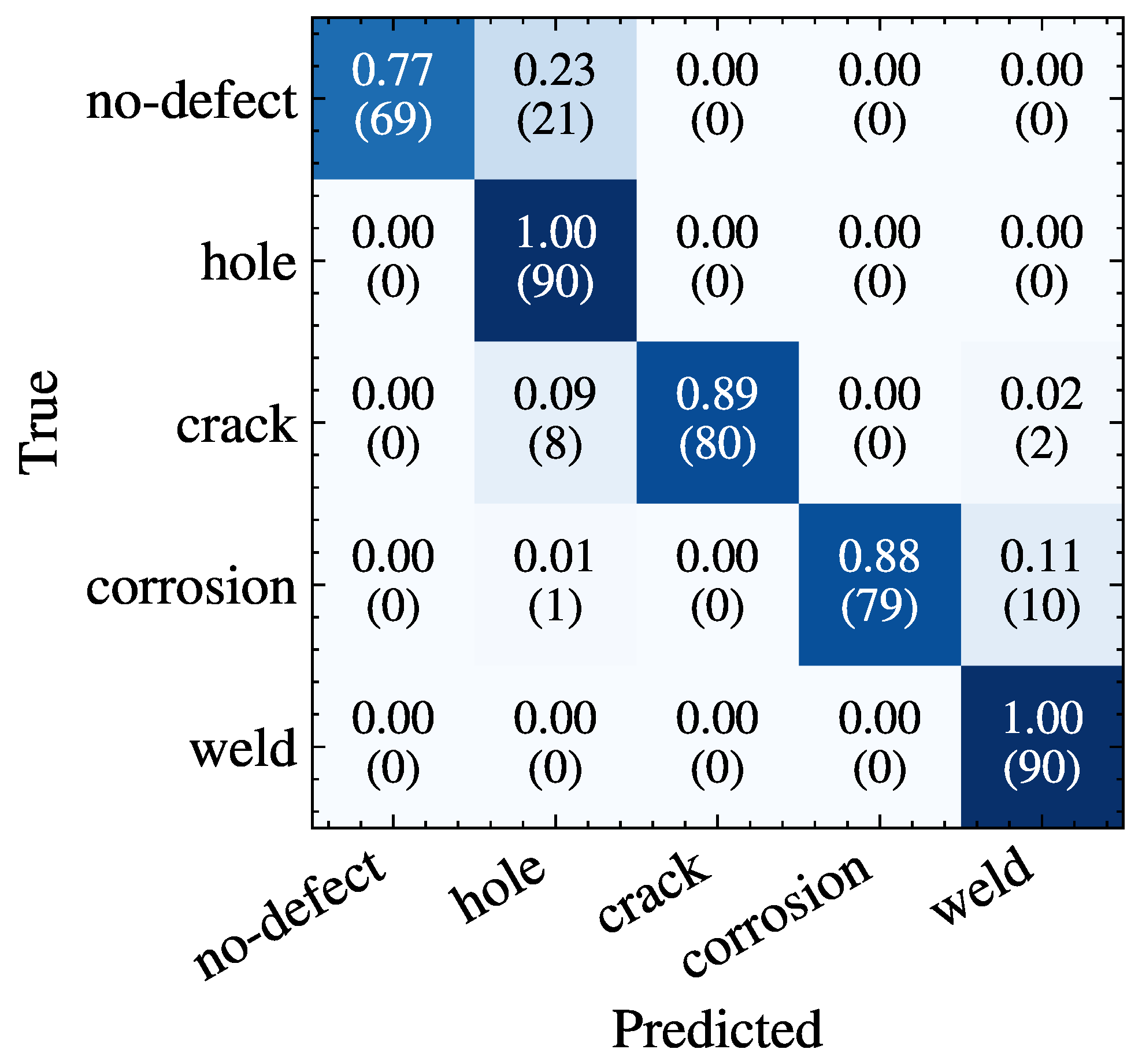
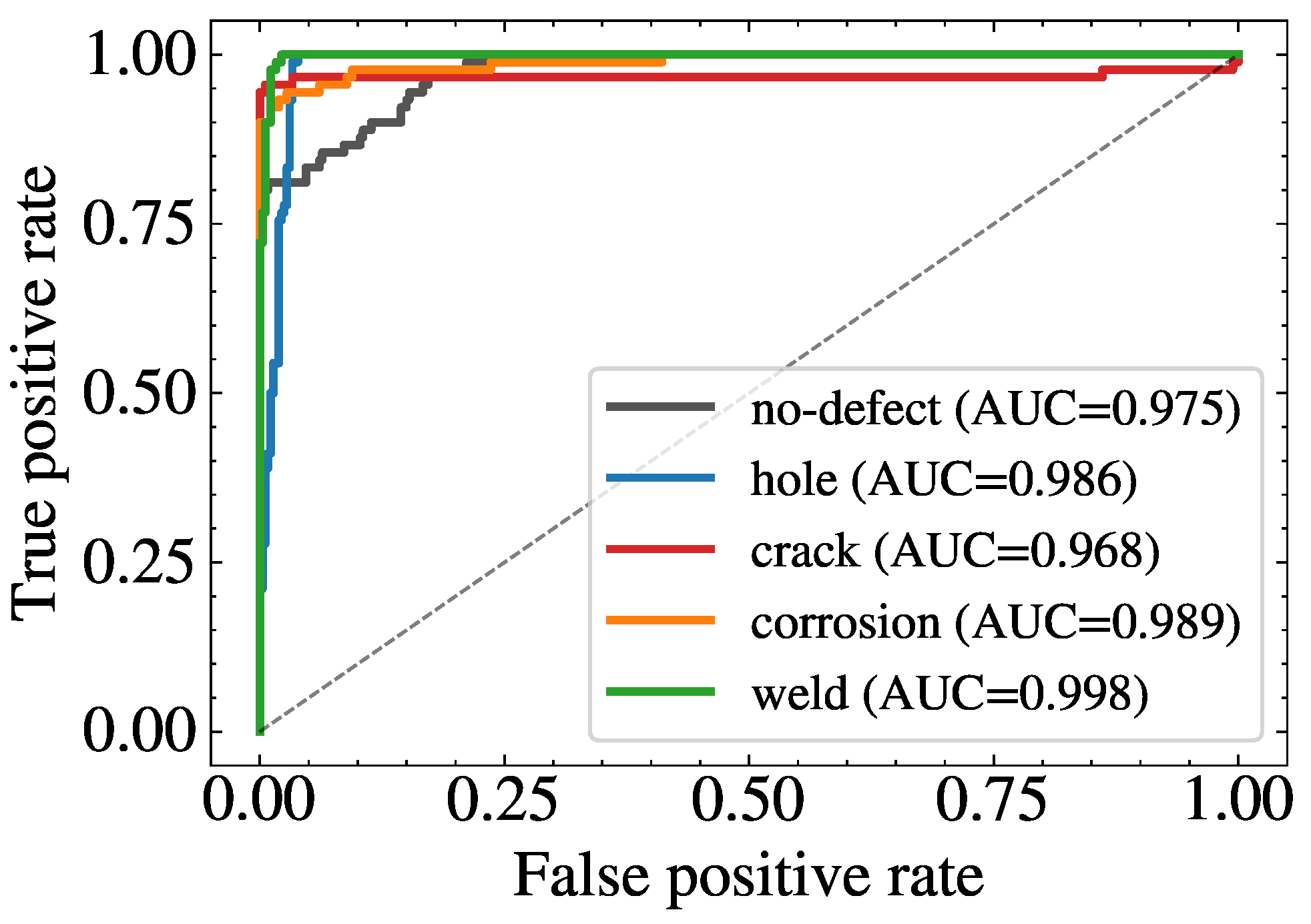
The framework rests on five design choices that simultaneously define the scope of the present study and the open questions for follow-up. Simulated data: All training and evaluation rely on the simulator in Section 4.1. The generalizability claims are deliberately scoped. Within the simulator’s drift envelope, the evaluation covers per-sample variation in the carrier frequency ($\pm 8\%$), group velocities ($\pm 15\%$), A0/S0 energy ratio ($\pm 80\%$), Tx–Rx distance ($\pm 10\%$), noise (SNR 25 dB), and five defect-size grades per class—a distribution-level test rather than a single condition. What is not covered, and is honestly stated here, includes independent variation in density and elastic modulus beyond the group-velocity proxy, physically different transducer designs, and measured industrial signals. The core claims of this work are, however, architectural: the logit-orthogonal bias-free head design is shown to be non-replaceable under ablation and to outperform the data-driven baselines on the same data—a controlled, fair comparison whose validity does not depend on simulator fidelity. Measured-data validation: We complement the simulator-based evaluation with an initial experimental campaign on a fully assembled EMAT chain. The rig is a 100 × 100 mm rail-grade steel plate instrumented with two EMAT probes at the standard $L=45$ mm separation; the four-stage Tx–Rx chain consists of a Tang Nano 9K FPGA driving a power board for pulse generation and trigger synchronisation, a flexible meander-coil EMAT probe, a front-end signal-amplifier module, and a multi-channel conditioning board with band-pass filtering and BNC output to the DAQ. On this rig we acquired 450 measured A-scans covering the same five defect classes as the simulator (no-defect, circular hole, crack, corrosion, weld) with nine size/severity groups per class and 10 repeated scans per group (90 scans per class); the model trained purely on simulated data was applied directly to these 450 scans with no fine-tuning on the measured set. The model attained a per-scan accuracy of 90.67% (408/450) and per-class one-vs-rest AUC ranging from 0.968 (crack) to 0.998 (weld); the per-class confusion matrix and ROC curves are reported in Figure 14 and Figure 15. The small gap to the simulated test accuracy (95.05%) is attributed to coupling and surface-roughness effects not modelled by the simulator. The classes that reach 100% recall (hole, weld) are precisely those whose corresponding physics head supervises a single dominant physical cue; the lower-recall classes (no-defect 76.7%, crack 88.9%, corrosion 87.8%) are the ones whose discriminating cues are most sensitive to coupling and surface roughness, both outside the simulator’s model. This pattern is consistent with the per-head knockout results in Section 5.2. Public bearing/acoustic datasets (CWRU, NASA bearing, FEMTO-ST) operate on a different modality and cannot serve as a direct transfer benchmark for Lamb-wave EMAT A-scans, which is why we built a dedicated rail-steel plate rig. Larger-scale measurements under varied Tx–Rx separations, temperatures, and field conditions are planned as future work.

Regarding the influence of simulation-to-experiment discrepancies on the physics heads, three observations apply. First, within the simulation the supervision is exact by construction: the physics-head targets are computed by the same physical formulas used to generate the signals, so there is no model mismatch inside the simulation; misspecification can only arise in the transfer to a real system. (i) The supervised quantities are first-order physical parameters—arrival time $\tau =L/c$, mode ratio, reflected-energy magnitude, and dispersive frequency shift—that are defined by the geometry, the material constants, and the wave velocities, and can be calibrated from a single direct-wave measurement; discrepancies in the fine waveform structure (mode coupling, surface-roughness scattering, probe nonlinearity) do not change their order of magnitude or their timing relations. (ii) Each physics head contributes a bias-free additive bias to its class logit, so a modestly biased supervision shifts the class margin rather than corrupting the classification; moreover, the training-time drift envelope ($\pm 15\%$ on the group velocities, $\pm 8\%$ on the carrier frequency) already exposes the heads to noisy targets, so the framework is robust to target-level uncertainty at the scale of the simulated drift. (iii) The knockout results show that each head is the dominant discriminator for its paired class; this remains valid as long as the calibrated quantity is directionally correct. The initial measured-data validation above provides a first confirmation of these three points (per-scan accuracy 90.67%, per-class AUC ≥ 0.97); a systematic comparison against the simulator’s drift envelope is ongoing. Five defect classes: The framework pre-assigns one physics head per defect class; extending to more classes requires a per-class physical quantity for each new class, which is not always available a priori. Class imbalance: The reported dataset is fully class-balanced (5000 samples per class). An earlier imbalanced variant (1000 no-defect samples) yielded a no-defect F1 of only 0.545; we evaluated the class-balanced variant and report it here, as it removes the minority-class bias without changing the defect-class data. Class-rebalanced sampling or focal loss were therefore not required. Single architecture family: The logit-orthogonal design is verified on the proposed backbone; whether the design transfers to other backbone families (Transformer, Mamba) is open. Simulator-side drift only: The training distribution itself spans the operating variability listed above as potential out-of-training conditions, via per-sample Gaussian drift applied independently to every generated signal: excitation conditions ($f_c\sim \mathcal{N}(0,8\%)$), material properties and plate thickness ($c_{\mathrm{S}0},c_{\mathrm{A}0}\sim \mathcal{N}(0,15\%)$ and the A0/S0 energy-ratio drift $\mathcal{N}(0,80\%)$), defect dimensions and severity (five size grades per class plus a continuous reflection amplitude sampled in $[0,1]$), noise level (additive white Gaussian noise at SNR $=25$ dB), and sensor configuration ($L\sim \mathcal{N}(0,10\%)$ Tx–Rx separation and probe-position jitter). The reported test accuracy is therefore a distribution-level test over these combined variations rather than a single-condition evaluation. What is not covered—independent variation in density and elastic modulus beyond the group-velocity proxy, and physically different transducer designs—requires measured data and is left to future work.

A separate note on the snapshot rule: as stated in Section 4.1, model and checkpoint selection are performed exclusively on the validation set, and the test set is evaluated once at the end of training; the corresponding numbers change by approximately $0.55$ pp on the proposed baseline under the corrected protocol (from $95.60\%$ under the original test-set selection to $95.05\%$ under validation-based selection), and the conclusions (above-80% baseline, below-80% ablations) do not depend on the snapshot rule.

6.6. Generalizability to Other Guided-Wave and Ultrasonic Modalities

The logit-orthogonal-head design is not specific to EMAT Lamb-wave A-scan. Three principles make it reusable for any one-dimensional industrial signal whose underlying scattering (or radiation, propagation, modulation) mechanism admits a per-class physical decomposition. First, the framework requires a simulator (or a calibrated physical model) that produces per-class physical quantities from raw inputs (e.g., arrival time, mode ratio, energy partition, frequency shift); once the simulator is in place, the four physics heads and the shared baseline can be wired against its outputs. Second, the framework requires a per-class physical quantity for each defect class; this is the strong inductive bias that limits the framework to modalities with a clear physics-to-class mapping. Third, the bias-free additive construction transfers verbatim: it is the only structural choice that guarantees non-replaceability, and it is independent of the backbone architecture. We have not yet validated these three transferability claims on a public benchmark (CWRU bearing, NASA bearing, FEMTO-ST), but the design is a concrete candidate for follow-up. Transferring from the rail-steel plate to a full rail cross-section requires accounting for the additional guided modes of the rail (e.g., 23 modes in U78CrV at 35 kHz [37]) and modal conversion; this is beyond the present plate-level scope and is left to future work.

From the perspective of industrial fault diagnosis for dynamic systems, the design is naturally aligned with the recent emphasis on transfer learning and explainable AI. The bias-free additive construction is backbone-agnostic, so a proposed head assembled against a different simulator (e.g. bearing vibration, gearbox acoustic emission, electrochemical impedance spectroscopy) can be plugged onto a Transformer or Mamba encoder without re-deriving the architecture; only the per-class physical-quantity definitions change. The head activations (Figure 5) and Grad-CAM heat-maps (Figure 6) give a deployment-side auditor a direct, time-localised view of which physical cue drove the classification, which is exactly the explainability contract that industrial fault-diagnosis systems are expected to honour. The shared-baseline residual CBM, in particular, isolates the residual capacity of the backbone from the class-specific physics decisions, so a future cross-modality transfer study can hold the head structure fixed and quantify how the residual capacity absorbs modality-specific structure.

7. Conclusions

We have presented a hybrid data–physics residual network (the proposed EMAT-PINN) for EMAT Lamb-wave A-scan defect classification, and have shown that the logit-orthogonal four-head design with bias-free additive projections makes each physics head structurally non-replaceable. On the 25,000-sample simulated benchmark, the proposed model reaches 95.05% test accuracy at only 0.195 M parameters, a +14.26-percentage-point margin over the strongest data-driven baseline ResNet1D (80.79%); every knockout ablation drops the model below the 80% hard-requirement threshold (68.79–75.55%), confirming that the four physics heads are non-replaceable by the residual capacity. The principal limitations are the reliance on simulated data as the primary training corpus, the small scale of the measured-data validation (450 scans from a single rig configuration), the fixed five-class taxonomy pre-assigned one physics head per defect class, and the use of a fully class-balanced dataset (1000 to 5000 no-defect samples) to address the minority-class F1 issue observed in an earlier imbalanced variant. Future work will scale the measured-data validation to larger campaigns under varied Tx–Rx separations, temperatures, and field conditions, extend the framework to more defect classes by adding heads, and assess cross-modality transfer to other one-dimensional industrial signals (guided-wave UT, vibration-based machine diagnostics, acoustic emission) on a public benchmark such as the CWRU bearing dataset.

References

1. Rose, J.L. Ultrasonic Guided Waves in Solid Media; Cambridge University Press: Cambridge, UK, 2014. [Google Scholar] [CrossRef] [Scilit]
2. Wilcox, P.D.; Lowe, M.; Cawley, P. Long Range Lamb Wave Inspection: The Effect of Dispersion and Modal Selectivity. In Review of Progress in Quantitative Nondestructive Evaluation; Springer: Boston, MA, USA, 1999; pp. 151–158. [Google Scholar]
3. Hirao, M.; Ogi, H. EMATs for Science and Industry: Non-Contacting Ultrasonic Measurements; Springer: New York, NY, USA, 2003. [Google Scholar] [CrossRef] [Scilit]
4. Viktorov, I.A. Rayleigh and Lamb Waves: Physical Theory and Applications; Plenum Press: New York, NY, USA, 1967. [Google Scholar]
5. Auld, B.A. Acoustic Fields and Waves in Solids; John Wiley & Sons: New York, NY, USA, 1973. [Google Scholar]
6. Song, T.; Peng, L.; Huang, S.; Huang, Z.; Feng, Q.; Sun, H. Non-Destructive Testing Technology for Shallow Subsurface Defects in Rails: A Review with Focus on Ultrasonic Surface Wave Methods. Sensors 2026, 26, 4614. [Google Scholar] [CrossRef] [Scilit] [PubMed]
7. Hu, S.; Zhai, G.; Lu, C.; Li, Z. Defect Localization in Switch Rail Foot with Variable Width via Spatial Mapping of SH0-like Guided Wave Time-of-Flight. NDT E Int. 2026, 162, 103743. [Google Scholar] [CrossRef] [Scilit]
8. Radosavljevic, S.; Rivero, A.; El Ouardi, A.; Flórez, S.R. Railway Track Defect Detection: From a Comprehensive Review of Methods to New Embedded System Modeling Perspectives. IEEE Trans. Instrum. Meas. 2026, 75, 3500325. [Google Scholar] [CrossRef] [Scilit]
9. Alleyne, D.N.; Cawley, P. The Interaction of Lamb Waves with Defects. IEEE Trans. Ultrason. Ferroelectr. Freq. Control 1992, 39, 381–397. [Google Scholar] [CrossRef] [Scilit] [PubMed]
10. Mallat, S. A Wavelet Tour of Signal Processing; Academic Press: San Diego, CA, USA, 1999. [Google Scholar]
11. Raissi, M.; Perdikaris, P.; Karniadakis, G.E. Physics-Informed Neural Networks: A Deep Learning Framework for Solving Forward and Inverse Problems Involving Nonlinear Partial Differential Equations. J. Comput. Phys. 2019, 378, 686–707. [Google Scholar] [CrossRef] [Scilit]
12. Karniadakis, G.E.; Kevrekidis, I.G.; Lu, L.; Perdikaris, P.; Wang, S.; Yang, L. Physics-Informed Machine Learning. Nat. Rev. Phys. 2021, 3, 422–440. [Google Scholar] [CrossRef] [Scilit]
13. Cuomo, S.; Di Cola, V.S.; Giampaolo, F.; Rozza, G.; Raissi, M.; Zabaras, N. Scientific Machine Learning through Physics-Informed Neural Networks: Where We Are and What’s Next. J. Sci. Comput. 2022, 92, 88. [Google Scholar] [CrossRef] [Scilit]
14. Krishnapriyan, A.; Gholami, A.; Zhe, S.; Kirby, R.; Mahoney, M.W. Characterizing Possible Failure Modes in Physics-Informed Neural Networks. In Proceedings of the Advances in Neural Information Processing Systems (NeurIPS), Virtual, 6–14 December 2021; Volume 34, pp. 26548–26560. [Google Scholar]
15. GB/T 34885-2017; Non-Destructive Testing—Electromagnetic Acoustic Testing—General Principles. National Standard of the People’s Republic of China: Beijing, China, 2017.
16. EN 16729-1; Railway Applications—Infrastructure—Non-Destructive Testing on Rails in Track—Part 1: Requirements for Ultrasonic Inspection and Evaluation Principles. European Committee for Standardization (CEN): Brussels, Belgium, 2016.
17. Maged, A.; Haridy, S.; Shen, H. Explainable Artificial Intelligence Techniques for Accurate Fault Detection and Diagnosis: A Review. arXiv 2024, arXiv:2404.11597. [Google Scholar]
18. Huang, N.E.; Shen, Z.; Long, S.R.; Wu, M.C.; Shih, H.H.; Zheng, Q.; Yen, N.C.; Tung, C.C.; Liu, H.H. The Empirical Mode Decomposition and the Hilbert Spectrum for Nonlinear and Non-Stationary Time Series Analysis. Proc. R. Soc. London Ser. A Math. Phys. Eng. Sci. 1998, 454, 903–995. [Google Scholar] [CrossRef] [Scilit]
19. Daubechies, I. Ten Lectures on Wavelets; SIAM: Philadelphia, PA, USA, 1992. [Google Scholar] [CrossRef] [Scilit]
20. Giurgiutiu, V. Structural Health Monitoring with PWAS; Academic Press: Oxford, UK, 2014. [Google Scholar]
21. Cortes, C.; Vapnik, V. Support-Vector Networks. Mach. Learn. 1995, 20, 273–297. [Google Scholar] [CrossRef] [Scilit]
22. Kiranyaz, S.; Ince, T.; Hamila, R.; Gabbouj, M. Convolutional Neural Networks for Patient-Specific ECG Classification. IEEE Trans. Biomed. Eng. 2015, 63, 664–675. [Google Scholar] [CrossRef] [Scilit] [PubMed]
23. He, K.; Zhang, X.; Ren, S.; Sun, J. Deep Residual Learning for Image Recognition. In Proceedings of the IEEE Conference on Computer Vision and Pattern Recognition (CVPR), Las Vegas, NV, USA, 27–30 June 2016; pp. 770–778. [Google Scholar] [CrossRef] [Scilit]
24. Hochreiter, S.; Schmidhuber, J. Long Short-Term Memory. Neural Comput. 1997, 9, 1735–1780. [Google Scholar] [CrossRef] [Scilit] [PubMed]
25. Cho, K.; van Merrienboer, B.; Gulcehre, C.; Bahdanau, D.; Bougares, F.; Schwenk, H.; Bengio, Y. Learning Phrase Representations using RNN Encoder–Decoder for Statistical Machine Translation. In Proceedings of the 2014 Conference on Empirical Methods in Natural Language Processing (EMNLP), Doha, Qatar, 25–29 October 2014; pp. 1724–1734. [Google Scholar] [CrossRef] [Scilit]
26. Vaswani, A.; Shazeer, N.; Parmar, N.; Uszkoreit, J.; Jones, L.; Gomez, A.N.; Kaiser, Ł.; Polosukhin, I. Attention Is All You Need. In Proceedings of the Advances in Neural Information Processing Systems (NeurIPS), Long Beach, CA, USA, 4–9 December 2017; Volume 30, pp. 5998–6008. [Google Scholar]
27. Lu, L.; Pestourie, R.; Yao, W.; Wang, Z.; Verdugo, F.; Johnson, S.G. Physics-Informed Neural Networks with Hard Constraints for Inverse Design. SIAM J. Sci. Comput. 2021, 43, B1105–B1132. [Google Scholar] [CrossRef] [Scilit]
28. Zhang, W.; Zhang, T.; Cui, G.; Pan, W. Intelligent Machine Fault Diagnosis Using Convolutional Neural Networks and Transfer Learning. IEEE Access 2022, 10, 50959–50971. [Google Scholar] [CrossRef] [Scilit]
29. Koh, P.W.; Liang, P. Understanding Black-box Predictions via Influence Functions. In Proceedings of the 34th International Conference on Machine Learning (ICML), Sydney, Australia, 6–11 August 2017; pp. 1885–1894. [Google Scholar]
30. Zhang, H.; Cheng, L.; Wen, R.; Zhang, Y.; Zhang, L.; Hermanns, H. SL-CBM: Enhancing Concept Bottleneck Models with Semantic Locality for Better Interpretability. In Proceedings of the AAAI Conference on Artificial Intelligence, Singapore, 20–27 January 2026; Volume 40, pp. 38093–38101. [Google Scholar] [CrossRef] [Scilit]
31. Szegedy, C.; Vanhoucke, V.; Ioffe, S.; Shlens, J.; Wojna, Z. Rethinking the Inception Architecture for Computer Vision. In Proceedings of the IEEE Conference on Computer Vision and Pattern Recognition (CVPR), Las Vegas, NV, USA, 27–30 June 2016; pp. 2818–2826. [Google Scholar] [CrossRef] [Scilit]
32. Chao, K.C.; Shih, Y.; Lee, C.H. A Novel Sensor-Based Label-Smoothing Technique for Machine State Degradation. IEEE Sens. J. 2023, 23, 10879–10888. [Google Scholar] [CrossRef] [Scilit]
33. Loshchilov, I.; Hutter, F. Decoupled Weight Decay Regularization. In Proceedings of the International Conference on Learning Representations (ICLR), New Orleans, LA, USA, 6–9 May 2019. [Google Scholar]
34. Kingma, D.P.; Ba, J. Adam: A Method for Stochastic Optimization. In Proceedings of the International Conference on Learning Representations (ICLR), San Diego, CA, USA, 7–9 May 2015. [Google Scholar] [CrossRef] [Scilit]
35. Loshchilov, I.; Hutter, F. SGDR: Stochastic Gradient Descent with Warm Restarts. In Proceedings of the International Conference on Learning Representations (ICLR), Toulon, France, 24–26 April 2017. [Google Scholar]
36. Paszke, A.; Gross, S.; Massa, F.; Lerer, A.; Bradbury, J.; Chanan, G.; Killeen, T.; Lin, Z.; Gimelshein, N.; Antiga, L.; et al. PyTorch: An Imperative Style, High-Performance Deep Learning Library. In Proceedings of the Advances in Neural Information Processing Systems (NeurIPS), Vancouver, BC, Canada, 8–14 December 2019; Volume 32, pp. 8024–8035. [Google Scholar]
37. Xu, X.; Wen, Z.; Ni, Y.; Shao, B.; Ma, X.; Pan, Z. Study on monitoring broken rails of heavy haul railway based on ultrasonic guided wave. Sci. Rep. 2024, 14, 8667. [Google Scholar] [CrossRef] [Scilit] [PubMed]
Figure 1. Lamb-wave group-velocity dispersion curves c ( f ) for the S0 and A0 modes. The marker indicates f c = 2.0 MHz, where c S 0 = 5.61 mm/ μ s and c A 0 = 4.22 mm/ μ s; the grey and green shaded bands represent the ± 1 σ sample-level drift envelopes of the S0 and A0 modes, respectively (Gaussian perturbation with σ = 15 % of the nominal group velocity).
Machines 14 01053 g001
Figure 2. Simulation setup and the five defect geometries considered in this work: (a) no-defect; (b) circular hole; (c) crack; (d) corrosion zone; (e) weld seam. The Tx–Rx probes are positioned on either side of the inspected region at L = 45 mm separation; the FEM mesh (light blue triangles) is the same gmsh-generated unstructured mesh used by the Lamb-wave forward solver.
Machines 14 01053 g002
Figure 3. Architecture overview of the proposed EMAT-PINN. This figure is a schematic overview of the proposed EMAT-PINN, not a layer-by-layer diagram. Arrows indicate the direction of data flow. It illustrates three design ideas: (i) the embedding of the physics prior into the network through four parallel physics heads, one per physical quantity ( amp / mode / arrive / disp ); (ii) the correspondence between each head and its paired defect class via the bias-free additive projection onto the class logit; and (iii) the use of a physics-constrained loss for gradient guidance. The blocks labelled “dual-pooling trunk” and “task heads” are conceptual placeholders. The precise layer configuration, the logit-construction equations ( 0 = b , k = b + fc add ( k ) ( e π ( k ) ) ), and the parameter count ( 0.195 M) are given in Table 2.
Machines 14 01053 g003
Figure 4. Four-head activation ablation on a single type-2 (crack) test sample under the proposed architecture: (a) raw A-scan; (b) amp head’s body activation (8-segment AdaptiveMaxPool, channel-mean, up-sampled to 1024 time points); (c) mode head’s activation on the same sample; (d) stacked sum of all four heads. The defect-to-direct energy ratio E def / E dir (defect-segment energy divided by direct-wave energy) is reported in each panel caption: the mode head scores highest because mode-discriminability is the dominant physical cue for crack classification, while raw gives the lowest.
Machines 14 01053 g004
Figure 5. Four-segment temporal decomposition under the proposed architecture, on a single type-2 (crack) test sample. (a) Raw A-scan with the S0 and A0 arrival markers ( 45 / c S 0 = 8.02 μ s, 45 / c A 0 = 10.66 μ s). (b) Eight-segment AdaptiveMaxPool activation of the amp (red) and mode (blue) heads, up-sampled to 1024 time points. (c) The arrive (green) and disp (orange) heads on the same axis. The four head activations are spatially correlated with the underlying scattering structure but differ in their amplitude and temporal focus, which is the signature of logit-orthogonal specialisation: each head responds to its own physics cue rather than to a shared representation.
Machines 14 01053 g005
Figure 6. Grad-CAM heat-maps (channel weights = backward gradient means over time, ReLU, up-sampled to 1024) on the four proposed physics heads. Top row: Raw A-scan of a single test sample per class (5 columns). Bottom row: Corresponding heat-maps on the matching heads— amp (no-defect, hole—reflected-energy cue), mode (crack—S0/A0 mode-ratio cue), arrive (corrosion—arrival-time cue), disp (weld—dispersive-frequency-shift cue). (a) no-defect, raw A-scan; (b) hole, raw A-scan; (c) crack, raw A-scan; (d) corrosion, raw A-scan; (e) weld, raw A-scan; (f) no-defect, amp head; (g) hole, amp head; (h) crack, mode head; (i) corrosion, arrive head; (j) weld, disp head.
Machines 14 01053 g006
Figure 7. Five-seed mean ± std test accuracy on the proposed model and the four data-driven baselines (seeds { 0 , 1 , 2 , 3 , 42 } , unified 60-epoch protocol); the 80 % reference line is shown for context. The error bars of the proposed model do not overlap those of any baseline, confirming that the + 15 –18 pp advantage over the strongest purely data-driven baseline is statistically significant rather than an artefact of a particular initialisation.
Machines 14 01053 g007
Figure 8. Proposed model’s baseline on the 5000-sample test set. Left: The five-class confusion. Right: The macro-averaged F1 is 95.05%; the per-class F1 values are 93.5% (no-defect), 92.9% (hole), 98.5% (crack), 96.7% (corrosion), and 96.3% (weld). (a) Row-normalised confusion matrix (acc 95.05 % ). (b) Per-class F1 (macro 95.05 % ).
Machines 14 01053 g008
Figure 9. Three cross-cutting views of the ablation study on the 5000-sample test set. (a) Scheme-level: The proposed baseline (dark blue) at 95.05 % together with its four knockout ablations, all collapsing below the 80 % hard-requirement threshold ( 68.79 75.55 % ). (b) Per-class knockout heat-map: Diagonal collapses with off-diagonal side-effects on no-defect/hole ( k o amp ) and no-defect/weld ( k o disp ) reveal that the four physics heads are entangled at the representation level. (c) Real-ablation accuracy across the four segments ( 71.05 / 75.55 / 71.55 / 68.79 % under the corrected val-best protocol), all below the 80 % threshold line, demonstrating that the proposed architecture cannot maintain industrial-acceptance accuracy when any single physics head is removed.
Machines 14 01053 g009
Figure 10. Training-process view of the proposed baseline (red, marker “∘”) and four REAL ablations (blue/green/purple/orange, marker “□”) on the unified 25,000-sample split (5 runs, 60 epochs each). In panel (c), solid and dashed curves denote test and validation accuracy, respectively; the gray dashed line marks the 80 % hard-requirement threshold and the black dotted line the 20 % five-class chance level. The deleted-segment residual loss in panel (d) is 0.42 1.04 , approximately one order of magnitude above its baseline value ( 0.009 0.051 ), indicating that, in our experiments, the missing head’s contribution is not absorbed by the residual capacity of the remaining three heads. (a) Train-loss trajectories (5 runs, 60 epochs). (b) Validation-loss trajectories (5 runs, 60 epochs). (c) Val (dashed) and test (solid) accuracy with reference lines. (d) Epoch-60 physics losses per run (hollow bar = deleted).
Machines 14 01053 g010
Figure 11. Knockout per-class diagnostics on the proposed baseline, 5000-sample test set. (a) Per-class F1 matrix under the four knockout ablations: the diagonal collapses to 0 for each ablation, confirming that each zeroed physics head carries the discriminative signal for its paired defect class. (b) Per-class accuracy under knockout (zero the head’s embedding at inference, weights unchanged): the diagonal collapses to exactly zero, and the k o phys row (all four heads zeroed simultaneously) collapses the model to predicting only no-defect ( 4.76 % overall).
Machines 14 01053 g011
Figure 12. Loss convergence of the proposed baseline over 60 epochs. Left (log scale): All five loss terms—cross-entropy L CE (black) drops from ∼0.96 to 0.24 , and the four physics losses are shown in colour. Right (linear scale): The four physics terms ( L amp , L mode , L arrive , L disp ) descend monotonically and converge to 0.051 / 0.024 / 0.009 / 0.009 , with L arrive and L disp reaching a near-steady state within the first 10 epochs. (a) All five loss terms, log scale. (b) Four physics losses, linear scale.
Machines 14 01053 g012
Figure 13. Four-segment residual scalar distribution on the proposed baseline (test set, n = 250 /class). Throughout the figure, colors denote the five classes: no-defect (gray), hole (red), crack (blue), corrosion (green), weld (orange). Top row (ad): Five-class overlaid histograms of the four head scalars pred amp / pred mode / pred arrive / pred disp with the dashed line marking the mean of the segment’s target class. Bottom row (eh): Per-class mean ± std bar chart for each segment. amp peaks on hole ( + 0.71 ) and weld ( + 0.72 ), confirming that the amp head encodes the reflected-energy magnitude as the primary cue for hole-vs-no-defect separation; mode is lowest on crack (+0.15), confirming the S0/A0 mode-ratio discrimination; arrive drops on corrosion (+7.99 vs. +8.28 baseline); disp varies mildly (+1.84 to +1.95). The class-discriminative information is distributed across all four segments, consistent with the ablation result that no single segment can be removed without breaking the model.
Machines 14 01053 g013
Figure 14. Measured-data validation on the rail-steel plate rig (450 A-scans, 5 classes × 9 size groups × 10 repeats): Per-scan confusion matrix, overall accuracy 90.67%; values in parentheses are sample counts.
Machines 14 01053 g014
Figure 15. Measured-data validation on the rail-steel plate rig (450 A-scans): Per-class one-vs-rest ROC curves, AUC 0.968–0.998.
Machines 14 01053 g015