Coordinated LADRC and GPOA-P&O MPPT for Robust Fault Ride-Through and Power Stability in Grid-Connected PV Systems

Abstract

Grid-connected photovoltaic (PV) systems require low-voltage ride-through (LVRT) to function reliably, particularly in the presence of symmetrical and asymmetric disturbances. Conventional PI-based control systems occasionally show limited resilience, particularly in the presence of distorted or imbalanced grid voltage. This paper proposes an enhanced LVRT control strategy for three-phase grid-connected PV systems by integrating a new rapid indirect Global Peak-Oriented Adaptive P&O MPPT method, referred to as (GPOA-P&O), with LADRC and DSOGI-FLL synchronization. The GPOA-P&O algorithm improves maximum power tracking by identifying the global peak and avoiding local maximum points, thereby reducing power fluctuations. Meanwhile, the cascaded LADRC controllers provide accurate voltage and current regulation, effectively suppressing DC-link overvoltage during grid disturbances. DSOGI-FLL ensures accurate positive-sequence phase-locking, enabling compliant reactive current injection even under severe voltage asymmetry, in accordance with grid-code requirements. The proposed method also eliminates second-order power oscillations and maintains constant inverter current regardless of fault severity. Case studies in 2024a MATLAB/Simulink and hardware-in-the-loop experimental platform demonstrate superior stability, fault ride-through capability, and grid-support performance compared to conventional approaches such as PI control and optimized SCSO-tuned PI.

1. Introduction

Increasing electricity demand and the depletion of fossil fuel resources have accelerated the transition toward distributed renewable energy systems [1,2]. As a result, distributed generation systems have gained increasing attention [3]. Among renewable energy sources, photovoltaic (PV) technology has emerged as one of the most promising options due to its scalability, environmental benefits, and wide range of applications, including rooftop systems and public infrastructure [4,5].

The penetration of PV generation into modern power grids has increased significantly, making the LVRT capability of PV power generation systems essential for safe and stable operation [6]. During grid faults, inverter disconnection can cause voltage instability at the point of common coupling (PCC) [7]. Therefore, grid codes require PV systems to stay connected during faults, support LVRT operation, and supply reactive current to help stabilize the grid voltage. Under voltage sags, whether symmetrical or asymmetrical, PV power output decreases abruptly, leading to DC-link overvoltage and potential overcurrent, which threaten inverter and grid stability [8]. Accordingly, accurate phase-locking, fault detection, and reliable LVRT control design have become critical research priorities [9].

To sustain the grid-connected power through failures and achieve LVRT, the authors in [10] advocate employing grid-connected converters for managed power management. The PV-MPPT function is abandoned in Ref. [11] to address the issue of voltage accretion at the DC-link during the low-voltage period. The authors in [12] do not effectively regulate the DC-side voltage; instead, it uses the open control loop of the voltage. A control system that lowers the DC-link voltage during the grid voltage decrease via the unloading circuit is introduced in [13]. Several studies have achieved LVRT by combining a crowbar circuit with reactive power control technique. According to the literature referenced previously, the DC-link voltage rise is mitigated by the unloading circuit within its low-voltage phase, and an overcurrent is prevented through restricting the utility grid inverter’s maximum output current [14].

The performance of the grid-connected PV inverter, a critical component of the PVPGS, has a direct influence on grid-voltage energy quality. To mitigate the effects of three-phase imbalances. including resonance contamination, frequency aberration, and sudden phase shifts, a PLL is required to monitor the grid voltage’s phases and frequencies in immediate effect. LVRT technology is therefore subject to stringent criteria for the grid-connected inverter system [15]. An SRF-PLL, or synchronized rotational framework, is frequently utilized at the PVPGS management systems [16]. To accomplish phase-locking objective, SRF-PLL tracks the synchronous rotational coordinate scheme and, at the optimal grid-voltage conditions, might be successfully phase-locked. In cases when the grid power becomes distortion or improperly unstable, the forward-sequence component of the voltage factor of the essential wave must be used as a point of reference. However, a negative-sequence element cannot be effectively controlled due to its limited bandwidth, which might result in a failure [17]. Some researchers have improved SRF-PLL in response to the issues. In order to eliminate oscillations in the electrical power, current, and voltage signals, they proposed the Improved PLL (IPLL) and Dual Improved PLL (DIPLL), that depends on a nonlinear adaptable filter [18]. Alternatively, the authors in [19] propose a decoupled Dual SRF-PLL, which can separate PNS components and achieve phase-locking in the event of an unbalanced power grid. However, the low-pass filtering becomes more complex and affects the reaction time of the system. In order to accomplish both phase sequence separation and phase lock, the PLL-based DSOGI (DSOGI-PLL) is presented in Ref. [20]. It generates signals that are quadrature and has a phase angle differential of 90. DSOGI-PLL does have several drawbacks, too, namely a poor dynamic response to abrupt frequency and phase changes. The study in [21] aims to enhance DSOGI by integrating a frequency-locked loop (FLL) with a frequency-adaptive mechanism.

Recent studies have further emphasized the importance of advanced LVRT and inverter-control strategies for grid-connected PV systems. Gholipour et al. [22] proposed an FCS-MPC-based LVRT strategy for a two-stage grid-connected PV system, focusing on fault detection, DC-link voltage regulation, overcurrent limitation, and active/reactive power support during grid faults. Gencer [23] introduced a machine-learning-assisted protection strategy to improve LVRT capability in grid-connected PV power plants by coordinating a DC chopper and fault current limiter [24]. In addition, Alharbi et al. [25] reviewed recent model predictive control methods for grid-connected PV inverters and highlighted their advantages in multi-objective regulation, dynamic response, and robustness. These studies confirm that coordinated MPPT, voltage/current regulation, synchronization, and grid-support control remain key research directions for improving PV system stability under grid disturbances.

The comparison in

Table 1. Comparison of related LVRT control methods for grid-connected PV systems.

Ref.	Method	System/Application	Main Contribution	Limitation/Gap
[1]	DRL-based controller	Grid-connected PV system	Improves LVRT capability using deep reinforcement learning	Requires complex training and broader validation
[2]	Grid-following/grid-forming converter control	Grid-connected PV converters	Compares LVRT performance under current limitations	Transient stability and current constraints remain challenging
[3]	RL-based adaptive sliding mode control	Multilevel grid-connected inverter	Enhances LVRT performance and robustness	Higher implementation complexity
[4]	Grid-forming LVRT strategy	Grid-forming converter	Considers current limitation and transient stability	Requires careful protection coordination
[25]	Grid-following/grid-forming mode control	Grid-connected converter	Supports symmetrical and asymmetrical fault ride-through	Synchronization under severe imbalance remains difficult
[6]	Single-stage PV LVRT control	Three-phase grid-connected PV system	Improves fault ride-through capability	Less flexible than two-stage PV structures
[8]	ADRC + DSOGI-FLL	Three-phase grid-connected PV system	Improves LVRT, synchronization, and disturbance rejection	MPPT performance and partial-shading response can be further improved
This work	GPOA-P&O MPPT + LADRC + DSOGI-FLL	Two-stage three-phase grid-connected PV system	Enhances LVRT under symmetrical and asymmetrical faults, suppresses power oscillations, regulates DC-link voltage, improves phase-locking, and supports reactive current injection	Future work may extend validation to broader hardware conditions, aging effects, and multi-inverter PV plants

summarizes recent LVRT control methods for grid-connected PV systems and highlights their main contributions and remaining limitations. DRL-based and reinforcement-learning-assisted controllers improve adaptability during grid faults but usually require complex training and broader validation [3]. Grid-following and grid-forming converter strategies enhance fault ride-through performance under current limitations, although transient stability and synchronization under severe unbalanced faults remain challenging [2,4,5]. Other studies improve LVRT through single-stage PV control, ADRC, and DSOGI-FLL synchronization, but issues related to partial shading, MPPT oscillations, DC-link overvoltage, and fast sequence extraction still need further improvement [6,8,9]. Compared to these methods, the present work combines GPOA-P&O MPPT, LADRC, and DSOGI-FLL to improve global MPPT tracking, suppress DC-link overvoltage, support reactive current injection, and enhance LVRT performance under both symmetrical and asymmetrical grid disturbances.

Controller selection is critical to ensure stable PV inverter operation, including accurate synchronization and sequence separation. Conventional PI/PID controllers often exhibit large transient errors, overshoot, and sluggish dynamic response due to integral action and their inherently linear structure. Under grid disturbances, these limitations can lead to voltage and current overshoot, triggering protection mechanisms and potentially causing system disconnection [26].

To address the obstacles of linear PID control, Jingqing Han proposed the ADRC method [27]. ADRC detects and rejects for internal and external disturbances instantaneously using input–output information, mitigating their impact before they affect system performance. Unlike PID, which reacts to error after it occurs, ADRC actively suppresses disturbances, enhancing dynamic response and robustness [28]. Owing to these advantages, ADRC has been extensively applied in wind energy systems, robotics, and unmanned aerial vehicles.

The key contributions of this work are summarized as follows:

• An enhanced LVRT control strategy is proposed for a double-stage grid-connected inverter, keeping the inverter current at 1 pu while limiting both balanced and unbalanced fault currents.
• ADRC replaces the classical PI controller to enhance dynamic response and reduce DC-link voltage oscillations during fault occurrence and recovery. In addition, DSOGI-FLL replaces the SRF-PLL to achieve accurate phase and frequency tracking with positive and negative-sequence extraction.
• The GPOA-P&O-ESF MPPT avoids local maxima and suppresses power oscillations. The ADRC controller limits DC-link overvoltage within ±5% of nominal, while DSOGI-FLL maintains phase-locking accuracy with a phase error below 0.5° under voltage asymmetry.
• The proposed control strategy ensures stable power injection and ripple-free DC-link voltage, even under unbalanced grid conditions.
• The proposed framework is validated through MATLAB/Simulink simulations and real-time HIL experiments, demonstrating superior stability, dynamic response, and fault ride-through capability compared to conventional PI and SCSO-tuned PI controllers.

The remainder of this study is organized as follows: Section 2 covers the LVRT concept and PV system requirements. Section 3 explains the modeling and architecture of grid-connected PVPG systems. Section 4 designs the proposed control strategies, Section 5 includes simulation results and discussions, and Section 6 contains conclusions.

2. LVRT Requirements in International Grid Codes

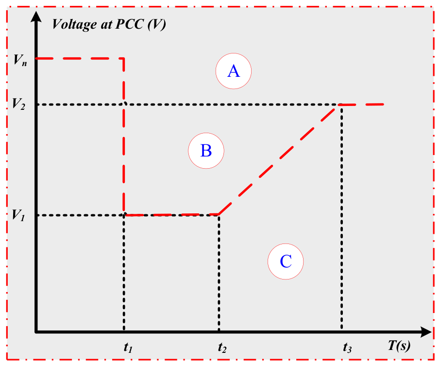
Grid codes (GCs) are technical specifications for connecting large-scale solar systems safely and reliably to power grids. Germany introduced the first GC for MV/HV solar plants in 2008 [29]; since then, Italy, China, South Australia, Spain, Africa, and Malaysia have established their own. Studies [30,31] review integration challenges and trends. LVRT requirements (Figure 1) define operating zones: A (normal), B (ride-through required), C (disconnection allowed).

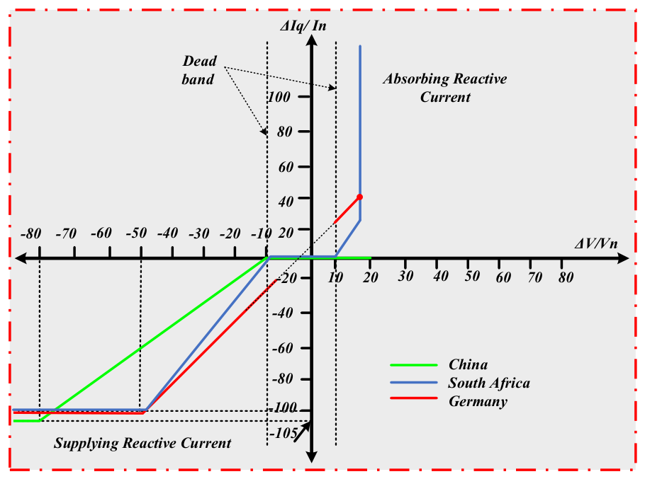
During grid faults, reactive power injection stabilizes voltage. Figure 2 displays the specifications for reactive current injections or absorbing for the grid coding (GC) of South Africa, Germany, and China. Germany mandates a 2% reactive current slope per 1% voltage drop, reaching full current for sags >50%. China requires a 1.5% slope for 0.2–0.9 pu dips, injecting 105% average current for drops >0.8 pu [32]. Unlike Germany and South Africa, China’s code requires no reactive absorption for overvoltage (>0.9 pu) [32]. A review of various requirements for linking PVPGS to the electrical grid in several nations is shown in

Table 2. A compilation of a few criterion for the power grid connection of PVPGS.

Country Grid Code (GC)	Rated Freq. (Hz)	Grid Freq. Boundaries (Hz)	Max Allowed Time	LVRT				HVRT
				Within Fault		After Fault		Through Voltage Swell
				V1 (%)	t2 (s)	V2 (%)	13 (s)	V%	t (s)
Germany (GC)	50	fg > 51.5	Disconnection (Trip)
		47.5 < fg < 51.5	Continue operate (No Trip)	0	0.15	90	1.5	120	0.1
		fg < 47.5	Disconnection (Trip)
Italy (GC)	50	ND	ND	0	0.2	85	1.5	125	0.1
Spain (GC)	50	fg > 51.5	Disconnection (Trip)
		47.5 < fg < 51.5	Continue operate (No Trip)	20	0.5	80	1	130	0.25
		48 < fg < 47.5	3 s
		fg < 47.5	Disconnection (Trip)
Australia (GC)	50	fg > 52	2 s	0	0.45	80	0.45	130	0.06
		47.5 < fg < 52	Continue operate (No Trip)
		fg < 47.5	2 s
China (GC)	50	fg > 50.2	2 min	20	0.15	90	2	ND	ND
		49.5 < fg < 50.2	Continue operate (No Trip)
		48 < fg < 49.5	10 min
		fg < 48	Characteristics of PV Inverter
Malaysia (GC)	50	fg > 52	Disconnection (Trip)	0	0.15	90	1.5	120	Continuous
		47 < fg < 52	Continue operate (No Trip)
		fg < 47	Disconnection (Trip)
S. Africa (GC)	50	fg > 52	4 s	0	0.15	85	2	120	0.15
		51 < fg < 52	60 s
		49 < fg < 51	Continue operate (No Trip)
		48 < fg < 49	60 s
		47 < fg < 48	10 s
		fg < 47	0.2 s

. Specific criteria including rated frequency, frequency limits, LVRT, and high-voltage (HVRT) ride through are the basis for these comparisons. Notably, frequencies between 3.5 and 2.5 Hz have the strictest limitations in relation to the assessed value [33].

3. Modeling and Architecture of Grid-Connected PVPG Systems

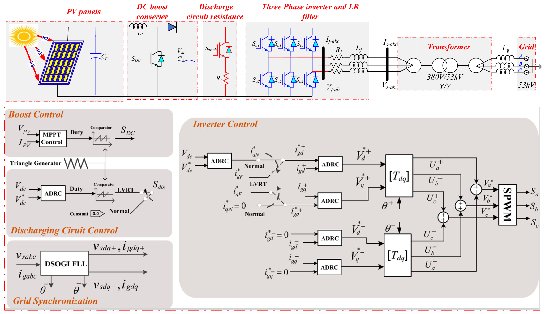
Figure 3 displays the whole block management structure and the dual-stage PVPGS design. A solar module, a step-up converter, a three-phase power inverter connected to a 35 kV boost transformer make up the system. The PV solar system model, the inverter power model in the event of unstable grid faults, the technique used to determine the reference currents for the positive- and negative-sequence components, the use of the LVRT’s controlling mechanism, and the calculation of the discharging circuit resistance are all provided to illustrate the control approach.

3.1. The PV Array Equivalent Model

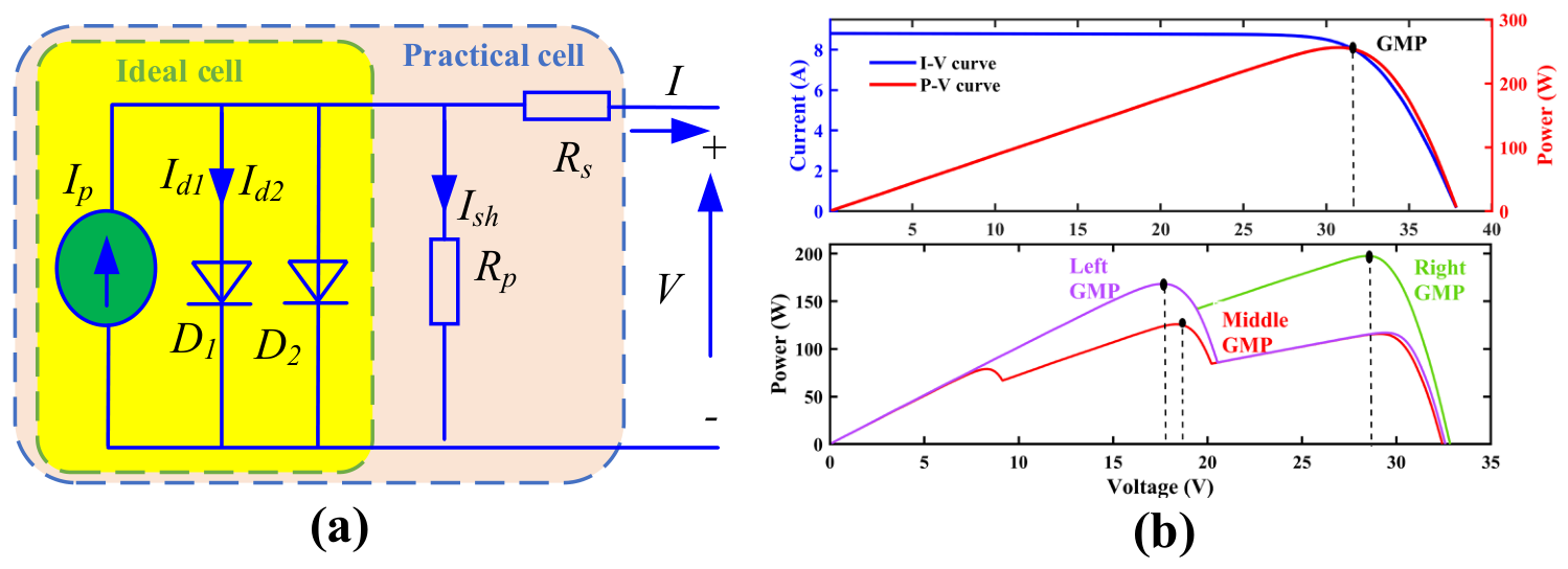
Single-diode or double-diode designs are regularly utilized to simulate the efficiency of solar panels. The double-diode model used for this investigation has an analogous circuit depicted in Figure 4. The P-N junction is represented by one diode (d₁), and the photocurrent by a current source (I_ph); the Joule effect losses through a series resistor (Rs), and the leakage current through a shunt resistor (Rsh). Based on Kirchhoff’s current law (KCL), Equations (1)–(5) provide the following calculation for a PV panel depending on the double-diode structure [34,35]:

$$I_{PVcell}=I_{ph}-I_{d1}-I_{d2}-I_{sh},$$

(1)

$$I_{ph}=(I_{sc}+K_i(T-T_{STC})){\displaystyle \frac{G}{G_{STC}}},$$

(2)

$$I_{d1}=I_{rs1}\left(\exp \left[{\displaystyle \frac{V_{cell}+R_s{I}_{cell}}{a_1{V}_{th}}}\right]-1\right),I_{d2}=I_{rs2}\left(\exp \left[{\displaystyle \frac{V_{cell}+R_s{I}_{cell}}{a_2{V}_{th}}}\right]-1\right),$$

(3)

$$I_{sh}={\displaystyle \frac{V_{PVcell}+R_s\cdot I_{PVcell}}{R_{sh}}},$$

(4)

$$I_{rs}=I_{st}{\left({\displaystyle \frac{T}{T_{STC}}}\right)}^3\exp \left[{\displaystyle \frac{q{E}_g}{Ak}}\left({\displaystyle \frac{1}{T_0}}-{\displaystyle \frac{1}{T}}\right)\right].$$

(5)

where a₁, a₂ are the diode idealization factor, I_rs1, I_rs2 stands for the diode reversal saturating currents, and Vth is the cell thermally voltage, which can be found using the formula Vth = kT/q, where k is the Boltzmann’s coefficient (1.38 × 10⁻²³ J) and q is the charge of the electron (1.602 × 10⁻¹⁹ C) [36,37]. The equivalent PV circuit and corresponding V-I/P-I curves are shown in Figure 4.

3.2. Inverter Modeling Under Asymmetrical Grid Failure

An asymmetrical voltage and current patterns, like PNS, occur when an unbalanced failure affects the power network. Almost none of the components are homopolar because of the PV inverter. Consequently, the following definition of perceived power in the event of an imbalanced grid breakdown is used as Equation (6).

$$S=P+jQ=1.5\left(v_{dq}^{+}{e}^{jwt}+v_{dq}^{-}{e}^{-jwt}\right)\cdot \left(i_{dq}^{+}{e}^{jwt}+i_{dq}^{-}{e}^{-jwt}\right)$$

(6)

where $v_{dq}^{+},v_{dq}^{-},i_{dq}^{+} and i_{dq}^{-}$ represent the voltage and current vectors defined in Equation (7).

$$\begin{array}{ll}{v}_{dq}^{+}=v_d^{+}+j{v}_q^{+},& v_{dq}^{-}=v_d^{-}+j{v}_q^{-},\\ i_{dq}^{+}=i_d^{+}+j{i}_q^{+},& i_{dq}^{-}=i_d^{-}+j{i}_q^{-}.\end{array}$$

(7)

In the d-q-axis, the sequences of $v_{dq}^{+},v_{dq}^{-}$ are in Equations (8) and (9):

$$\left[\begin{array}{c}{v}_d^{+}\\ v_q^{+}\\ 0\end{array}\right]={\displaystyle \frac{2}{3}}\left[\begin{array}{ccc}\cos (\theta )& \cos (\theta -{\displaystyle \frac{2\pi }{3}})& \cos (\theta +{\displaystyle \frac{2\pi }{3}})\\ \sin (\theta )& \sin (\theta -{\displaystyle \frac{2\pi }{3}})& \sin (\theta +{\displaystyle \frac{2\pi }{3}})\\ {\displaystyle \frac{1}{2}}& {\displaystyle \frac{1}{2}}& {\displaystyle \frac{1}{2}}\end{array}\right]\left[\begin{array}{c}{v}_a^{+}\\ v_b^{+}\\ v_c^{+}\end{array}\right]$$

(8)

$$\left[\begin{array}{c}{v}_d^{-}\\ v_q^{-}\\ 0\end{array}\right]={\displaystyle \frac{2}{3}}\left[\begin{array}{ccc}\cos (-\theta )& \cos (-\theta -{\displaystyle \frac{2\pi }{3}})& \cos (-\theta +{\displaystyle \frac{2\pi }{3}})\\ \sin (-\theta )& \sin (-\theta -{\displaystyle \frac{2\pi }{3}})& \sin (-\theta +{\displaystyle \frac{2\pi }{3}})\\ {\displaystyle \frac{1}{2}}& {\displaystyle \frac{1}{2}}& {\displaystyle \frac{1}{2}}\end{array}\right]\left[\begin{array}{c}{v}_a^{-}\\ v_b^{-}\\ v_c^{-}\end{array}\right]$$

(9)

Here, θ denotes the utility grid voltage’s phase angle as determined by D-SOGI-FLL, as shown in Figure 3. Furthermore, the stationary reference coordinates’ PNS voltages are shown through $v_a^{+},v_b^{+},v_c^{+} and v_a^{-},v_b^{-},v_c^{-}$.

Active power P and reactive power Q are the two components of apparent power that are separated using Equations (10) and (11).

$$P=P_0+P_{c2}\cos (2\omega t)+P_{s2}\sin (2\omega t)$$

(10)

$$Q=Q_0+Q_{c2}\cos (2\omega t)+Q_{s2}\sin (2\omega t)$$

(11)

where P_c2, P_s2, Q_c2, and Q_s2 denote the fluctuating elements of the active and reactive powers through the two-times grid-frequency component, and P₀ and Q₀ are the average components of those powers. After that, their expressions are provided by Equation (12):

$$\begin{array}{l}{P}_0=1.5(v_d^{+}{i}_d^{+}+v_q^{+}{i}_q^{+}+v_d^{-}{i}_d^{-}+v_q^{-}{i}_q^{-}),\\ P_{c2}=1.5(v_d^{-}{i}_d^{+}+v_q^{-}{i}_q^{+}+v_d^{+}{i}_d^{-}+v_q^{+}{i}_q^{-}),\\ P_{s2}=1.5(v_q^{-}{i}_d^{+}-v_d^{-}{i}_q^{+}-v_q^{+}{i}_d^{-}+v_d^{+}{i}_q^{-}),\\ Q_0=1.5(v_q^{+}{i}_d^{+}-v_d^{+}{i}_q^{+}+v_q^{-}{i}_d^{-}-v_d^{-}{i}_q^{-}),\\ Q_{c2}=1.5(v_q^{-}{i}_d^{+}-v_d^{-}{i}_q^{+}+v_q^{+}{i}_d^{-}-v_d^{+}{i}_q^{-}),\\ Q_{s2}=1.5(v_d^{+}{i}_d^{-}+v_q^{+}{i}_q^{-}-v_d^{-}{i}_d^{+}-v_q^{-}{i}_q^{+})\end{array}$$

(12)

In Equation (12), there is a multivariable coupling that is not reversible and maybe expressed as a matrix of 6 × 4 coefficients as shown in Equation (13).

$$\left[\begin{array}{c}{P}_0\\ Q_0\\ P_{c2}\\ P_{s2}\\ Q_{c2}\\ Q_{s2}\end{array}\right]={\displaystyle \frac{2}{3}}\left[\begin{array}{cccc}{v}_d^{+}& v_q^{+}& v_d^{-}& v_q^{-}\\ v_q^{+}& -v_d^{+}& v_q^{-}& -v_d^{-}\\ v_d^{-}& v_q^{-}& v_d^{+}& v_q^{+}\\ v_q^{-}& -v_d^{-}& -v_q^{+}& v_d^{+}\\ v_q^{-}& -v_d^{-}& v_q^{+}& -v_d^{+}\\ -v_d^{-}& -v_q^{-}& v_d^{+}& v_q^{+}\end{array}\right]\left[\begin{array}{c}{i}_d^{+}\\ i_q^{+}\\ i_d^{-}\\ i_q^{-}\end{array}\right]$$

(13)

Six parameters exist in this expression, while only four degrees of freedom are available; thus, not all can be determined instantaneously. The difference between the current regulators is obtained from (14) based on the PV inverter power requirement under the PNSC strategy.

$${\left[\begin{array}{c}{i}_d^{+}\\ i_q^{+}\\ i_d^{-}\\ i_q^{-}\end{array}\right]}_{ref}={\displaystyle \frac{2}{3}}\left[\begin{array}{cc}{\displaystyle \frac{v_d^{+}}{\mathrm{E}1}}& {\displaystyle \frac{v_q^{+}}{\mathrm{E}2}}\\ {\displaystyle \frac{v_q^{+}}{\mathrm{E}1}}& -{\displaystyle \frac{v_d^{+}}{\mathrm{E}2}}\\ -\mathrm{K}{\displaystyle \frac{v_d^{-}}{\mathrm{E}1}}& +\mathrm{K}{\displaystyle \frac{v_d^{-}}{\mathrm{E}2}}\\ -K{\displaystyle \frac{v_d^{-}}{\mathrm{E}1}}& -\mathrm{K}{\displaystyle \frac{-v_d^{+}}{\mathrm{E}2}}\end{array}\right]{\left[\begin{array}{c}P\\ Q\end{array}\right]}_{ref}$$

(14)

where

$$E1={(v_d^{+})}^2+{(v_q^{+})}^2-K({(v_d^{-})}^2+{(v_q^{-})}^2),$$

(15)

$$E2={(v_d^{+})}^2+{(v_q^{+})}^2+K({(v_d^{-})}^2+{(v_q^{-})}^2)$$

(16)

Additionally, parameter K ∈ {0, 1, −1} in (14)–(16) determines the controller mode:

• K = 0: Eliminates negative-sequence current, allowing double-frequency power oscillations.
• K = 1: Suppresses active power oscillations using P_c2 and P_s2.
• K = −1: Suppresses reactive power oscillations using Q_c2 and Q_s2.

In this study, K = 0 is adopted to eliminate negative-sequence current while tolerating double-frequency power oscillations and preventing current overshoot.

3.3. Sequence Current Reference Generation $i_{dref}^{+},i_{dref}^{-}$

The DSOGI-FLL block separates the positive and negative sequences (PNSs). Two control loops regulate the positive- and negative-sequence currents, ensuring that the inverter output currents in the dq frame accurately track their reference values. These references are derived from (14) according to the control objective defined by parameter K. When K = 0, the positive current references are obtained from (17).

$${\left[\begin{array}{c}{i}_d^{+}\\ i_q^{+}\end{array}\right]}_{ref}={\displaystyle \frac{2}{3}}\left[\begin{array}{cc}{\displaystyle \frac{v_d^{+}}{{(v_d^{+})}^2+{(v_q^{+})}^2}}& {\displaystyle \frac{v_q^{+}}{{(v_d^{+})}^2+{(v_q^{+})}^2}}\\ {\displaystyle \frac{v_q^{+}}{{(v_d^{+})}^2+{(v_q^{+})}^2}}& {\displaystyle \frac{-v_d^{+}}{{(v_d^{+})}^2+{(v_q^{+})}^2}}\end{array}\right]{\left[\begin{array}{c}P\\ Q\end{array}\right]}_{ref}$$

(17)

The injection of negative-sequence current helps minimize the inverter output current. Accordingly, the negative-sequence current control loop is defined by (18).

$$i_{dref}^{-}=0,i_{qref}^{-}=0$$

(18)

The voltage-oriented control (VOC) technique aligns the grid voltage with the d-axis, setting $v_q^{+}$ to zero, which causes Equation (17) to become Equation (19):

$$i_{dref}^{+}={\displaystyle \frac{P_{ref}}{1.5v_d^{+}}},i_{qref}^{+}={\displaystyle \frac{Q_{ref}}{1.5v_d^{+}}}$$

(19)

where the target values of active and reactive power in this case are P_ref and Q_ref, respectively. These values are determined based on the following analysis.

To avoid overcurrent, the grid-injected reactive power should be kept within the rated capacity of the system. During voltage sags, the grid cannot absorb the full PV power, increasing the apparent power demand. Therefore, the inverter current is limited using the maximum apparent power S_max, which depends on the voltage-sag depth as (20).

$$Smax=1.1{\displaystyle \frac{v_d^{+}}{v_d}}S$$

(20)

Here, S stands for the perceived power of the system, and $v_d^{+}/v_d$ for the voltage-sag depth. The coefficient is set at 1.1 according to the inverter’s nominal and optimum current capacity proportion.

The reference for adding reactive power into electrical grid is specified through the Chinese grid code and is calculated using Equation (21):

$$\left\{\begin{array}{cc}{Q}_{ref}=0\hfill & \hfill V>0.9\hfill \\ Q_{ref}=1.5\ast S\ast (0.9-V)\hfill & \hfill 0.2<V<0.9\hfill \\ Q_{ref}=1.05\ast S\hfill & \hfill V<0.2\hfill \end{array}\right.$$

(21)

Here, V, which is represented by Equation (22), is the grid phase voltage with the lowest value per unit.

$$V=min\left\{V_{sa}{V}_{sb}{V}_{sc}\right\}$$

(22)

The reference active power that must be supplied in order to avoid inverter overcurrent damage is therefore determined as Equation (23):

$$P_{ref}=\sqrt{{\mathrm{Smax}}^2-Q_{ref}^2}$$

(23)

Throughout grid faults, the reference active power is limited and not all generated PV power can be transferred to the utility grid. The surplus energy accumulates in the DC-link, causing overvoltage and threatening inverter stability. Therefore, a discharging circuit is added to regulate the DC-link voltage. As shown in Figure 3, the excess energy is dissipated through resistor R₁, whose value is given in (24).

$$R_1={\displaystyle \frac{V_{dc}^2}{S-P}}$$

(24)

4. Mathematic Modeling of the Proposed Control Approaches

4.1. Linear ADRC Design

Linear active disturbance-rejection control (LADRC), proposed by Gao, simplifies the practical implementation of ADRC by using a linear extended state observer (LESO) and linear state error feedback. In contrast to nonlinear ADRC, LADRC does not use the nonlinear fal() function or nonlinear state error feedback. Therefore, the observer and controller gains can be determined through a bandwidth-based tuning method, which improves parameter-selection simplicity and reproducibility.

To illustrate the ADRC principle, an n-order nonlinear time-varying system with one input u(t) and one output y(t) is considered, as expressed in Equation (25).

$$y^n(t)=f\left(y(t),y^1(t),y^2(t),\dots ,y^{n-1}(t),u(t)\right)+d(t)+b_0.u(t)$$

(25)

where d(t) represents the external disturbance, (b₀) is a known system parameter, and ($f\left(y(t),y^1(t),y^2(t),\dots ,y^{n-1}(t),u(t)\right)$) denotes the unknown internal dynamics of the system.

The unknown internal dynamics and external disturbances are collectively treated as the total disturbance $f(t)=f\left(y(t),y^1(t),y^2(t),\dots ,y^{n-1}(t),u(t)\right)+d(t)$, which must be estimated and compensated by the controller. Accordingly, the system equation can be rewritten as follows:

$$y^n(t)=f(t)+b_0.u(t)$$

(26)

Instead of deriving an explicit analytical expression for f(t), ADRC estimates the total disturbance online, which greatly reduces the controller’s dependence on an accurate system model. In this approach, f(t) is estimated in real time by the ESO and then compensated through a suitable control input u(t).

$$\left\{\begin{array}{l}{z}_1=y,\\ z_1=\dot{y},\dots ,z_n=y^{n-1}\\ z_{n+1}=f.\end{array}\right.$$

(27)

By differentiating f and defining it as an additional state variable, $\dot{f}=h$ in Equation (27) can be expressed as

$$\begin{array}{l}\dot{z}=Az+Bu+Eh,\\ y=Cz,\end{array}$$

(28)

where

$$\begin{array}{l}\left(z={[z_1,z_2,\dots ,z_n,z_{n+1}]}^T\right)\\ A^{(n+1,n+1)}=\left[\begin{array}{ccccc}0& 1& 0& \dots & 0\\ 0& 0& 1& \dots & 0\\ ⋮& ⋮& ⋮& \ddots & ⋮\\ 0& 0& 0& \dots & 1\\ 0& 0& 0& \dots & 0\end{array}\right],\\ B^{(n+1,1)}={[10\dots 00]}^T,\\ E^{(n+1,1)}={[00\dots 01]}^T,\\ B^{(1,n+1)}={[10\dots 00]}^T.\end{array}$$

(29)

A full-order Luenberger state observer can then be constructed as follows:

$$\begin{array}{l}\dot{\widehat{z}}(t)=A\widehat{z}+Bu+L(y-\widehat{y}),\\ \widehat{y}=C\widehat{z},\end{array}$$

(30)

where L denotes the observer gain vector.

The observation error between the actual state z and the estimated state $\widehat{z}$ can be expressed as follows:

$$e(t)=z-\widehat{z}.$$

(31)

Consequently, the error-estimation dynamics can be written as

$$\dot{e}=(A-LC)e,$$

(32)

where $\widehat{z}$

$$A-LC=\left[\begin{array}{ccccc}-{\beta }_1& 1& 0& \dots & 0\\ -{\beta }_2& 0& 1& \dots & 0\\ ⋮& ⋮& ⋮& \ddots & ⋮\\ -{\beta }_n& 0& 0& \dots & 1\\ -{\beta }_{n+1}& 0& 0& \dots & 0\end{array}\right].$$

(33)

To ensure asymptotic convergence of the estimation error, i.e., e→0 as t→∞, and to guarantee proper observer performance, the gain matrix L must be selected such that (A − LC) is a Hurwitz matrix. In other words, all roots of the ESO characteristic polynomial P_ESO(s) must have negative real parts:

$$P_{ESO}(s)=\det \left(s{I}_{n+1}-(A-LC)\right)=s^{n+1}+{\beta }_1{s}^n+{\beta }_2{s}^{n-1}+\dots +{\beta }_{n}s+{\beta }_{n+1}$$

(34)

Observer gains are commonly selected using a pole-placement method. In ESO design, a trade-off is required between fast state tracking and sensitivity to noise or disturbance estimation. A faster ESO can estimate and compensate the total disturbance more rapidly through the control law. Therefore, the observer poles are usually placed farther to the left of the system poles in the s-plane, which gives the ESO a wider bandwidth. However, excessively high observer bandwidth may amplify measurement noise and negatively affect system performance.

Considering these constraints, the ESO cutoff frequency ωo is selected to provide a suitable settling time while avoiding excessive noise amplification. Accordingly, the (n + 1) observer poles are placed at −ωo, as follows:

$$P_{ESO}(s)=s^{n+1}+{\beta }_1{s}^n+{\beta }_2{s}^{n-1}+\dots +{\beta }_{n}s+{\beta }_{n+1}={(s+{\omega }_o)}^{n+1}$$

(35)

Thus, the observer gains can be expressed as follows:

$${\beta }_i={\displaystyle \frac{(n+1)!}{(n+1-i)!i!}}{\omega }_o^i$$

(36)

When (A − LC) is stable, the estimated state ${\widehat{z}}_1,{\widehat{z}}_2,\dots ,{\widehat{z}}_n$ represents the output y and its derivatives up to order n − 1, while ${\widehat{z}}_{n+1}$ estimates the total disturbance f(t). The estimated disturbance can then be rapidly rejected through the following control law:

$$u(t)={\displaystyle \frac{u_0(t)-{\widehat{z}}_{n+1}(t)}{b_0}},$$

(37)

Accordingly, the system in Equation (26) can be transformed into

$$y^n(t)=f(t)-{\widehat{z}}_{n+1}(t)+u_0(t)$$

(38)

The system can be reduced to an n-order integrator when ${\widehat{z}}_{n+1}$ accurately estimates $f({\widehat{z}}_{n+1}\approx f)$ and its derivatives:

$$y^n(t)=u_0(t)$$

(39)

Therefore, the resulting system can be controlled using an appropriate state-feedback control law:

$$u_0(t)=k_1\left(r(t)-y(t)\right)+k_2\left(\dot{r}(t)-\dot{y}(t)\right)+\dots +k_n\left(r^{n-1}(t)-y^{n-1}(t)\right),$$

(40)

where r(t) denotes the reference signal.

Given that (${\widehat{z}}_1(t),{\widehat{z}}_2(t),\dots ,{\widehat{z}}_n(t)$) accurately estimates ($y(t),\dots ,y^{n+1}(t)$) and its derivatives, the final control law can be formulated as follows:

$$u(t)={\displaystyle \frac{k_1\left(r(t)-\widehat{z}(t)\right)+\dots +k_n\left(r^{n-1}(t)-{\widehat{z}}_n(t)\right)-{\widehat{z}}_{n+1}(t)}{b_0}}=k_0\left(\widehat{r}(t)-\widehat{z}(t)\right),$$

(41)

where

$$\begin{gathered} \widehat{r}(t)={[r(t)\dot{r}(t),\dots ,r^{n-1}(t)0]}^T, \\ {K}_0={\displaystyle \frac{[k_1,k_2,\dots ,k_{n}1]}{b_0}} \end{gathered}$$

(42)

The linear ADRC can therefore be formulated as follows:

$$\left\{\begin{array}{l}\dot{\widehat{z}}(t)=A\widehat{z}(t)+Bu(t)+L[y(t)-C\widehat{z}(t)]=(A-LC)\widehat{z}(t)+Bu(t)+Ly(t),\\ u(t)=K_0[\widehat{r}(t)-\widehat{z}(t)].\end{array}\right.$$

(43)

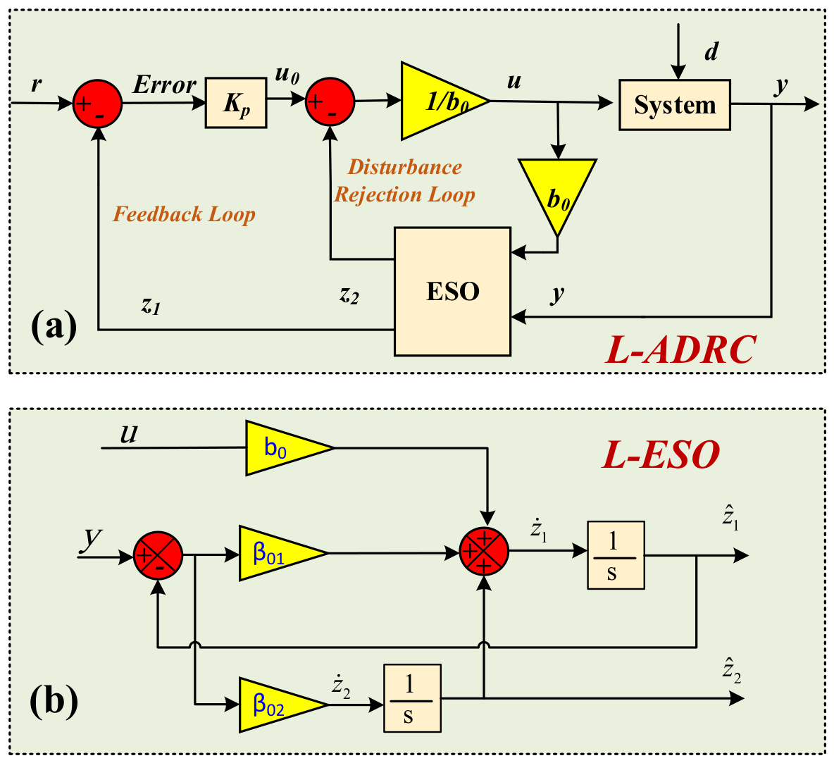
In this study, the observer bandwidth is chosen higher than the controller bandwidth to ensure fast disturbance estimation while avoiding excessive noise amplification. The outer voltage loops are assigned lower bandwidths because the capacitor-voltage dynamics are relatively slow, whereas the inner current loops are assigned higher bandwidths to achieve faster current regulation. Specifically, the PV voltage and DC-link voltage loops use K_p = 60, β₀₁ = 480, and β₀₂ = 57,600, while the PV current and grid current loops use K_p = 300, β₀₁ = 2400, and β₀₂ = 1,440,000. The scheme of the proposed LADRC is shown in Figure 5a, and the LESO pole-placement method and bandwidth-based gain selection are provided in Figure 5b [38].

4.2. Stability Analysis

Stability analysis is performed to verify the convergence of the estimation-error dynamics and to ensure the stability of the closed-loop control system. Define the estimation error as $e=z-\widehat{z}$. The error dynamics can then be expressed as $\dot{e}=(A-LC)e$. The observer gain L is selected so that the matrix A − LC has eigenvalues with negative real parts, thereby guaranteeing observer stability. The closed-loop stability can then be examined by substituting the control input u into the system dynamics:

$${\dot{x}}_n=f(x)+b(x)u+d(t)$$

(44)

$$u=-{\displaystyle \frac{1}{b(x)}}\left[{\widehat{z}}_{n+1}+{\displaystyle \sum _{i=1}^n{k}_i(x_i-{\widehat{z}}_i)}\right]$$

(45)

Substituting u into the system equation yields

$${\dot{x}}_n=f(x)+b(x)\left(-{\displaystyle \frac{1}{b(x)}}\left[{\widehat{z}}_{n+1}+{\displaystyle \sum _{i=1}^n{k}_i(x_i-{\widehat{z}}_i)}\right]\right)+d(t)$$

(46)

Assuming perfect estimation, i.e., $z=\widehat{z}$, the system reduces to

$${\dot{x}}_n={\displaystyle \sum _{i=1}^n{k}_i(x_i-{\widehat{z}}_i)}$$

(47)

The feedback gains k_i are selected to achieve the desired closed-loop pole placement and ensure stable system response [37,38].

4.3. LADRC Parameter Tuning and Sensitivity Analysis

The LADRC parameters were selected using the bandwidth-based tuning method. For the first-order LADRC structure adopted in this work, the controller gain is determined by the desired controller bandwidth ω_c, while the extended state observer gains are calculated from the observer bandwidth ωo as β₀₁ = 2ωo and β₀₂ = ${\omega }_o^2$. Since the current dynamics are faster than the capacitor-voltage dynamics, the inner PV current and grid current loops were assigned higher controller bandwidths than the outer PV voltage and DC-link voltage loops. Specifically, the PV voltage and DC-link voltage loops used ω_c = 60 rad/s and ωo = 240 rad/s, resulting in β₀₁ = 480 and β₀₂ = 57,600. The PV current and grid current loops used ω_c = 300 rad/s and ωo = 1200 rad/s, resulting in β₀₁ = 2400 and β₀₂ = 1,440,000. The observer bandwidth was selected as approximately four times the controller bandwidth to provide fast disturbance estimation while avoiding excessive noise amplification. These values were verified through simulation and HIL tests under normal, fault, and post-fault conditions.

The sensitivity analysis in

Table 3. Sensitivity analysis of LADRC controller and observer bandwidths under LVRT operating conditions.

Case	Controller Bandwidth	Observer Bandwidth	DC-Link Voltage Overshoot	Settling Time	Current Ripple	LVRT Stability	Observation
Low bandwidth	(0.5 ωc)	(0.5 ωo)	High	Long	Low	Stable but slow	Slow disturbance rejection and delayed recovery
Moderate–low bandwidth	(0.75 ωc)	(0.75 ωo)	Medium	Medium–long	Low	Stable	Improved stability, but recovery is still slower
Nominal bandwidth	(ωc)	(ωo)	Low	Short	Low–medium	Stable	Best compromise between response speed and robustness
Moderate–high bandwidth	(1.25 ωc)	(1.25 ωo)	Low–medium	Short	Medium	Stable	Faster response, but ripple begins to increase
High bandwidth	(1.5 ωc)	(1.5 ωo)	Low	Very short	High	Stable but less robust	Higher noise sensitivity and increased voltage/current ripple

shows that reducing the LADRC bandwidth slows the disturbance-rejection capability, leading to larger DC-link voltage deviation and longer settling time during LVRT operation. In contrast, excessively increasing the bandwidth improves response speed but increases voltage/current ripple and noise sensitivity; therefore, the nominal bandwidth was selected as the best compromise between fast dynamic response, low overshoot, limited ripple, and stable LVRT performance.

4.4. Grid Synchronization Using DSOGI-FLL

Under unbalanced grid-voltage conditions, the waveform amplitude and frequency become distorted, which reduces the effectiveness of direct PLL tracking. Therefore, the phase angle and frequency of the positive-sequence component must be extracted to accurately represent the grid voltage. Based on the classical symmetrical component theory, the positive-sequence voltage components can be extracted as follows [8] in Equation (48).

$$\left[\begin{array}{c}{v}_a^{+}\\ v_b^{+}\\ v_c^{+}\end{array}\right]={\displaystyle \frac{1}{3}}\left[\begin{array}{ccc}1& a^2& a\\ a& 1& a^2\\ a^2& a& 1\end{array}\right]\left[\begin{array}{c}{v}_a\\ v_b\\ v_c\end{array}\right]$$

(48)

where ɑ is constant constraint distinct e^(j2π/3).

The Clarke Transformation is used for obtaining the positive-sequence voltage factor in Equation (49).

$$\left[\begin{array}{c}{v}_{\alpha }^{+}\\ v_{\beta }^{+}\end{array}\right]={\displaystyle \frac{2}{3}}\left[\begin{array}{ccc}1& -{\displaystyle \frac{1}{2}}& -{\displaystyle \frac{1}{2}}\\ 0& -{\displaystyle \frac{\sqrt{3}}{2}}& -{\displaystyle \frac{\sqrt{3}}{2}}\end{array}\right]\left[\begin{array}{c}{v}_a^{+}\\ v_b^{+}\\ v_c^{+}\end{array}\right]={\displaystyle \frac{1}{2}}\left[\begin{array}{cc}1& -q\\ q& 1\end{array}\right]\left[\begin{array}{c}{v}_{\alpha }\\ v_{\beta }\end{array}\right]$$

(49)

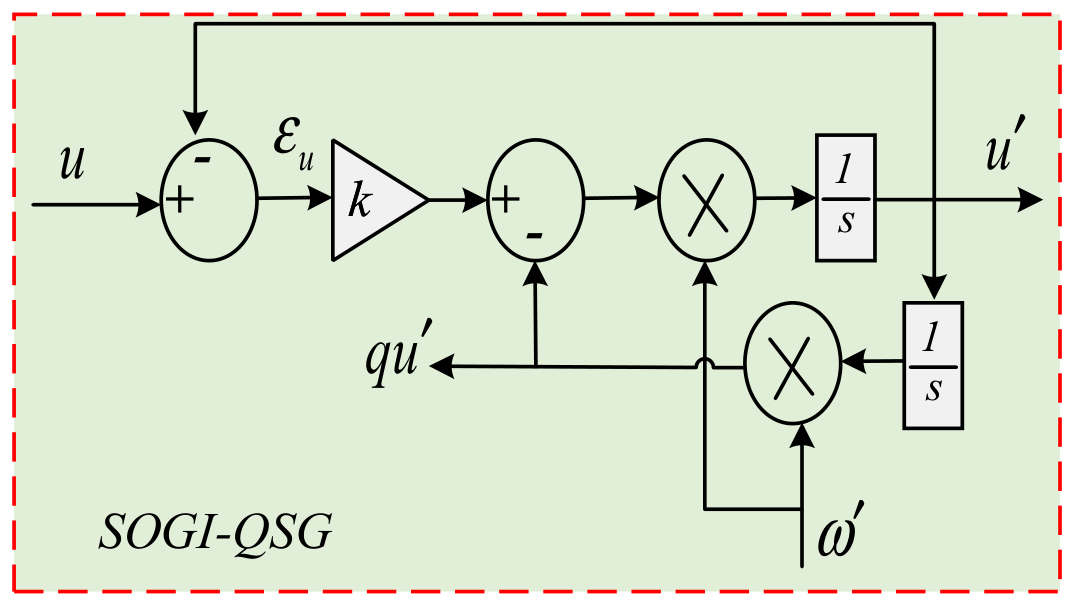
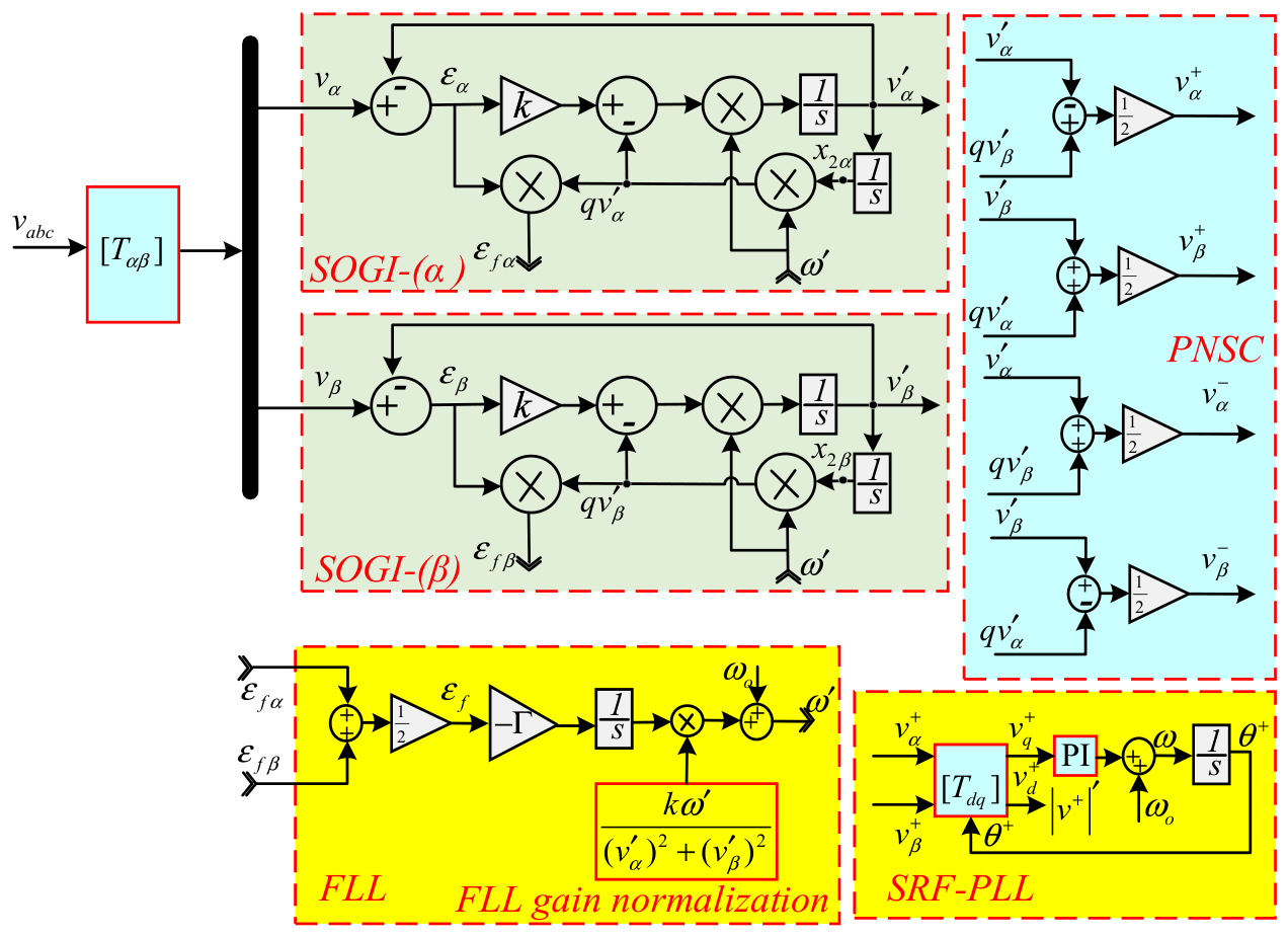
Here, q = e^jπ/2 acts as a phase shift operator that introduces a 90-degree lag from the original phase. To achieve this 90-degree phase shift, a QSG is required. The inverse Park transform (IPT), T/4 delay, and adaptive notch filter (ANF) are commonly used to generate this signal. However, these methods rely on sine and cosine functions, increasing algorithm complexity, response time, and sensitivity to noise. In contrast, the SOGI provides a simpler structure based on a phase-shifting circuit. The corresponding SOGI structure is shown in Figure 6.

In Figure 6, the input signal u represents the component of rotational voltage (either u_α or u_β). The final, $u^{\prime }$ and $q{u}^{\prime }$, are two orthogonal voltage signals with a 90° phase difference between them. The error among the supplied signal u and final signal $u^{\prime }$ is represented by symbol ε_u, while ${\omega }^{\prime }$ represents the predictable angular frequency. Equations (50)–(52) provide the relevant transfer function:

$$G(\mathrm{s})={\displaystyle \frac{u^{\prime }}{k{\epsilon }_u}}(\mathrm{s})={\displaystyle \frac{{\omega }^{\prime }s}{s^2+{{\omega }^{\prime }}^2}}$$

(50)

$$D(\mathrm{s})={\displaystyle \frac{u^{\prime }}{u}}(\mathrm{s})={\displaystyle \frac{k{\omega }^{\prime }s}{s^2+k{\omega }^{\prime }s+{{\omega }^{\prime }}^2}}$$

(51)

$$Q(\mathrm{s})={\displaystyle \frac{q{u}^{\prime }}{u}}(\mathrm{s})={\displaystyle \frac{k{{\omega }^{\prime }}^2}{s^2+k{\omega }^{\prime }s+{{\omega }^{\prime }}^2}}$$

(52)

In this formulation, (G(s)) represents the overall transfer function of the system, while (D(s)) and (Q(s)) denote the band-pass and low-pass filtering functions used to generate the orthogonal output signals. The filter bandwidth is determined solely by the coefficient (k), rather than by the input signal frequency. This property gives the SOGI structure natural frequency-adaptive behavior, making it well-suited for rapid frequency changes.

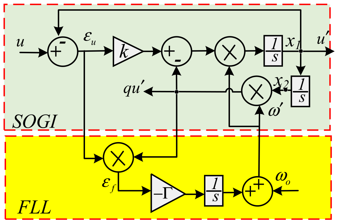
To improve phase and frequency tracking under voltage imbalance or variation, an FLL is incorporated. The SOGI-FLL operates on u_α or u_β voltage components and consists of an SOGI block with a frequency adaptation unit, as shown in Figure 7.

In comparison to the standalone SOGI, the addition of the FLL introduces a feedback mechanism where the FLL receives the quadratic voltage $q{u}^{\prime }$ and the voltage error ε_u from SOGI. A closed-loop control framework is created by estimating the frequency error ε_f using a controller and integrators by the gain coefficient Γ, and then feeding the calculated angular frequency ${\omega }^{\prime }$ directly to the SOGI. This feedback loop enables precise frequency adaptation by continuously correcting ${\omega }^{\prime }$, effectively eliminating frequency drift. As a result, the frequency error signal ε_f converges to zero, attaining frequency lock.

The following Equations (53) and (54) are an expression for the SOGI-FLL’s state-space:

$$\dot{x}=\left[\begin{array}{c}{\dot{x}}_1\\ {\dot{x}}_2\end{array}\right]=Ax+Bu=\left[\begin{array}{cc}-k{\omega }^{\prime }& {{\omega }^{\prime }}^2\\ 1& 0\end{array}\right]\left[\begin{array}{c}{x}_1\\ x_2\end{array}\right]+\left[\begin{array}{c}k{\omega }^{\prime }\\ 0\end{array}\right]u$$

(53)

$$y=\left[\begin{array}{c} u^{\prime }\\ q{u}^{\prime }\end{array}\right]=Cx=\left[\begin{array}{cc}1& 0\\ 0& {\omega }^{\prime }\end{array}\right]\left[\begin{array}{c}{x}_1\\ x_2\end{array}\right]$$

(54)

where x denotes the state vector and y represents the output vector. The dynamic behavior of the SOGI-FLL is described by Equation (55):

$${\omega }^{\prime }=-\mathsf{\Gamma }{x}_2{\omega }^{\prime }(u-x_1)$$

(55)

Because positive and negative sequences share the same frequency in an unbalanced grid, a conventional SOGI cannot separate them. Therefore, a DSOGI is used for sequence decoupling. The voltage at the grid terminal is first converted to u_α and u_β using the Clarke transform, filtered by SOGI blocks to produce orthogonal signals, and then processed by PNSC for sequence extraction. As shown in Figure 8, the DSOGI-FLL includes frequency and phase feedback loops for accurate tracking under grid disturbances.

5. Power Converter Control Design

ADRC is used to control the dual-stage PV power generating mechanism, which improves consistency and instantaneous performance. Under dynamic operating conditions, ADRC enables reliable control over the voltage at DC-link and grid-connected current.

5.1. Design of the ADRC-Based DC–DC Converter Controller

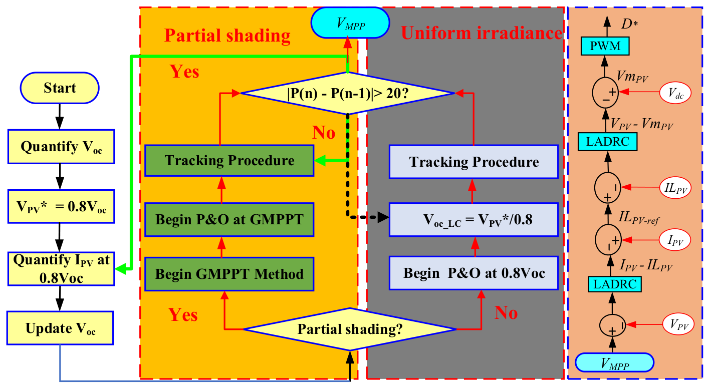
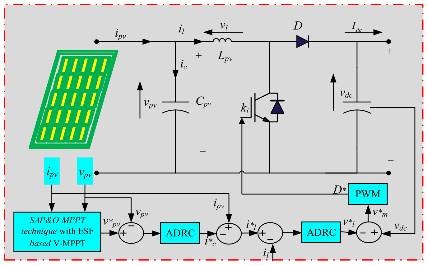
This work adopts a two-stage MPPT scheme to ensure stable PV operation under changing environmental conditions. As demonstrated in Figure 9, the tracked voltage point (Vmpp) is initially obtained utilizing the GPOA-P&O MPPT method. Then, an improved LADRC-based cascaded control structure regulates the PV voltage and current to accurately track the optimal operating point and maximize power extraction [39].

5.1.1. Voltage-Based MPPT Using the Proposed GPOA-P&O Method

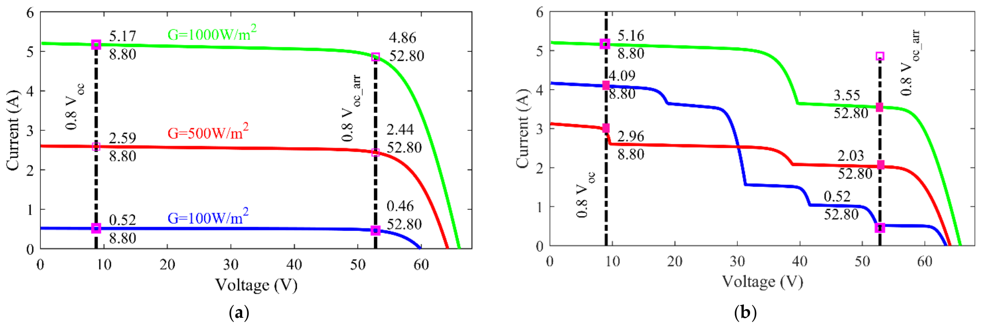
Voltage-assisted MPPT is used to determine the tracked voltage point (V_mpp) associated with the maximum power point. Owing to its reliability and tracking capability, the proposed GPOA-P&O-assisted V-MPPT strategy is utilized, as illustrated in Figure 10. Partially shaded (PS) is identified using Equations (56) and (57), which distinguish uniform irradiance conditions from shaded operating conditions.

$$G_1={\displaystyle \frac{I_{0.8Voc}}{I_{SC\_STC}}}\cdot G_{STC}$$

(56)

$$G_2={\displaystyle \frac{I_{0.8Voc\_array}}{I_{MPP\_STC}}}\cdot G_{STC}$$

(57)

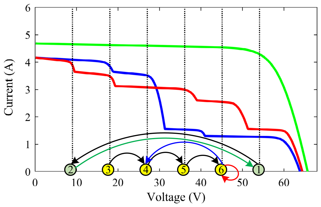
Here, (I0.8Voc_arr) denotes the current corresponding to approximately (0.8Voc_arr), while (I0.8V_oc) represents the current near (0.8Voc). Because the PV modules include two bypass diodes, (Voc) refers to the OCV of half of one module, while (Voc_arr) represents the open-circuit voltage of the three series-linked modules. Under uniform irradiance conditions, (G1) and (G2) are nearly identical, as shown in Figure 10.

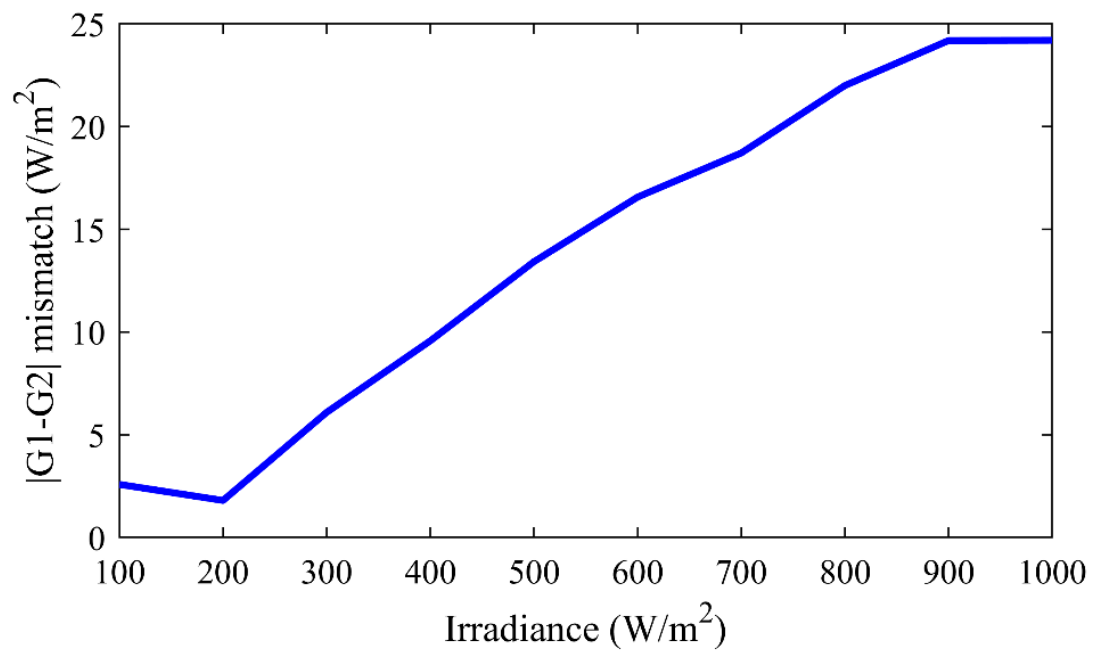
Although (|G1 − G2|) changes with irradiance under uniform conditions, its value remains within a predefined limit. As shown in Figure 11, the mismatch error for the three SW85W modules stays below 25 W/m² under UC. Therefore, Equations (58) and (59) are used to distinguish between uniform irradiance and PS circumstances.

$$\left|G_1-\right.\left.G_2\right|<30 \mathrm{without} \mathrm{PS} (\mathrm{UC})$$

(58)

$$\left|G_1-\right.\left.G_2\right|>30 \mathrm{With} \mathrm{PS}$$

(59)

Figure 12 illustrates the I–V characteristics under partial-shading conditions. Consider the red curve as a prime instance, and the calculated values of (G1) and (G2) are obtained using Equations (60) and (61).

$$G_1={\displaystyle \frac{I_{0.8Voc}}{I_{SC\_STC}}}\cdot G_{STC}={\displaystyle \frac{2.96}{5.2}}\cdot 1000=569.2{ \mathrm{W}/\mathrm{m}}^2$$

(60)

$$G_2={\displaystyle \frac{I_{0.8Voc\_array}}{I_{MPP\_STC}}}\cdot G_{STC}={\displaystyle \frac{2.03}{4.86}}\cdot 1000=417.69{ \mathrm{W}/\mathrm{m}}^2$$

(61)

As revealed in Figure 12, using the initial rate of Voc_arr removes the need to assume that the MPP has been previously detected. This makes the proposed method more flexible and suitable for different initial operating conditions.

At the beginning, the algorithm identifies the lower-limit open-circuit voltage (Voc_arr,LC}). The currents (I0.8Voc_arr) and (I0.8Voc) are formerly measured and stored to determine (G₁) and (G₂). After that, (Voc_arr,UD}) is updated using Equation (62). The PV generator is considered to operate under uniform irradiance only when the condition in Equation (63) is satisfied.

$$V_{op\_array\_update}=V_{op\_array\_LC}+\alpha \left({\displaystyle \frac{n_{s}K.T}{q}}\right).N_s.\ln \left({\displaystyle \frac{G_1}{G_{STC}}}\right)$$

(62)

$$V_{op\_array\_LC}={\displaystyle \frac{V_{MPP\_array}}{0.8}}$$

(63)

The partial-shading detection process compares the currents measured at (0.8Voc) and (0.8Voc_arr) as soon as the power variation surpasses 10%, as shown in Conditions 1–2 of Figure 13. If no PS is sensed, the conventional P&O algorithm is applied directly. When partial shading is identified, the GMPPT procedure is activated, where currents are sampled at several voltage points, Conditions 3–6, to locate the global peak before applying P&O. By avoiding unnecessary scanning steps, the GMPPT process improves tracking speed.

5.1.2. ADRC-Based V-MPPT Control Design

Since the PV voltage at the maximum power point changes only slightly under varying operating conditions, voltage-based MPPT is an effective choice. To improve tracking accuracy and robustness, an LADRC-assisted cascaded voltage–current control loop is introduced. This controller forces (V_pv) to follow the V_MPP tracked point, while the DC step-up converter is used to determine the voltage oscillations in Equation (64).

$${\displaystyle \frac{d{V}_{pv}}{dt}}={\displaystyle \frac{1}{C_{pv}}}{i}_c$$

(64)

Based on the ADRC standard form given in Equation (65), the corresponding controller is formulated as Equation (64).

$$\left\{\begin{array}{l}{f}_{V_{pv}}(\cdot )=-C_{pv}+b_{0V_{pv}},\\ b_{0V_{pv}}={\displaystyle \frac{1}{C_{pv}}},\\ u=i_c\end{array}\right.$$

(65)

The inner control-loop dynamics responsible for regulating the inductor current are described by Equation (66).

$${\displaystyle \frac{d{i}_l}{dt}}={\displaystyle \frac{1}{L}}{v}_l$$

(66)

Therefore, the ADRC strategy for the control loop is expressed in Equation (67).

$$\left\{\begin{array}{l}{f}_{i_l}(\cdot )=-{\displaystyle \frac{1}{L}}+b_{0i_l},\\ b_{0i_l}={\displaystyle \frac{1}{L}},\\ u=v_l\end{array}\right.$$

(67)

5.2. Inverter Control Using Linear ARDC Design

The control aims to regulate grid-side currents and stabilize the DC-Link voltage for active/reactive power control. Voltage-oriented control (VOC) aligns the grid voltage in d-axis (v_sd = Vs and v_sq = 0) and setting reactive power to zero ensures unity power factor. Figure 3 shows the control scheme.

5.2.1. Grid-Side Current Control

Under normal grid conditions, the grid-side currents flowing through the LC filter resistance (Rf) and inductance (Lf) are expressed in the rotating (d)-(q) reference frame through Equations (68) and (69).

$${\displaystyle \frac{d{i}_{gd}}{dt}}=-{\displaystyle \frac{R_f}{L_f}}{i}_{gd}+{\displaystyle \frac{1}{L_f}}{v}_{sd}-{\omega }_g{i}_{gq}-{\displaystyle \frac{1}{L_f}}{v}_{fd}$$

(68)

$${\displaystyle \frac{d{i}_{gq}}{dt}}=-{\displaystyle \frac{R_f}{L_f}}{i}_{gq}+{\displaystyle \frac{1}{L_f}}{v}_{sq}-{\omega }_g{i}_{gd}-{\displaystyle \frac{1}{L_f}}{v}_{fq}$$

(69)

Here, v_fd, v_fq represent the inverter output voltages, while v_sd, v_sq denote the grid utility voltages, and ω_g is the grid’s angular frequency. Under unbalanced grid-fault circumstances, Equations (68) and (69) are reformulated as Equation (70):

$$\left\{\begin{array}{l}{L}_f{\displaystyle \frac{{{di}_{gdq}}^{+}}{dt}}=-R_f{i_{gdq}}^{+}-{\omega }_g{i_{gdq}}^{+}+{v_{sdq}}^{+}-{v_{fdq}}^{+}\\ L_f{\displaystyle \frac{d{i_{gdq}}^{-}}{dt}}=-R_f{i_{gdq}}^{-}-{\omega }_g{i_{gdq}}^{-}+{v_{sdq}}^{-}-{v_{fdq}}^{-}\end{array}\right.$$

(70)

By decoupling the positive and negative-sequence components, Equation (70) can be rearranged into the ADRC canonical form as Equation (71):

$${\displaystyle \frac{d}{dt}}\left[\begin{array}{c}{i}_{gd}^{+}\\ i_{gq}^{+}\\ i_{gd}^{-}\\ i_{gq}^{-}\end{array}\right]=\left[\begin{array}{c}{f}_{gd}^{+}(\cdot )\\ f_{gq}^{+}(\cdot )\\ f_{gd}^{-}(\cdot )\\ f_{gq}^{-}(\cdot )\end{array}\right]+{\left[\begin{array}{c}{b}_{0\_gd}^{+}\\ b_{0\_gq}^{+}\\ b_{0\_gd}^{-}\\ b_{0\_gq}^{-}\end{array}\right]}^t\left[\begin{array}{c}{u}_{gd}^{+}\\ u_{gq}^{+}\\ u_{gd}^{-}\\ u_{gq}^{-}\end{array}\right]$$

(71)

Equation (72):

$$\left[\begin{array}{c}{f}_{gd}^{+}(\cdot )\\ f_{gq}^{+}(\cdot )\\ f_{gd}^{-}(\cdot )\\ f_{gq}^{-}(\cdot )\end{array}\right]={\displaystyle \frac{1}{L_f}}\left[\begin{array}{c}-R_f{i}_{gd}^{+}-{\omega }_g{i}_{gd}^{+}+v_{sd}^{+}-(1+L_f{b}_{0\_gd}^{+})v_{fd}^{+}\\ -R_f{i}_{gq}^{+}-{\omega }_g{i}_{gq}^{+}+v_{sq}^{+}-(1+L_f{b}_{0\_gq}^{+})v_{fq}^{+}\\ -R_f{i}_{gd}^{-}-{\omega }_g{i}_{gd}^{-}+v_{sd}^{-}-(1+L_f{b}_{0\_gd}^{-})v_{fd}^{-}\\ -R_f{i}_{gq}^{-}-{\omega }_g{i}_{gq}^{-}+v_{sq}^{-}-(1+L_f{b}_{0\_gq}^{-})v_{fq}^{-}\end{array}\right]$$

(72)

Equation (73):

$$\left[\begin{array}{c}{u}_{gd}^{+}\\ u_{gq}^{+}\\ u_{gd}^{-}\\ u_{gq}^{-}\end{array}\right]=\left[\begin{array}{c}{v}_{fd}^{+}\\ v_{fq}^{+}\\ v_{fd}^{-}\\ v_{fq}^{-}\end{array}\right],{\left[\begin{array}{c}{b}_{0\_gd}^{+}\\ b_{0\_gq}^{+}\\ b_{0\_gd}^{-}\\ b_{0\_gq}^{-}\end{array}\right]}^t=\left[{\displaystyle \frac{1}{L_f}} {\displaystyle \frac{1}{L_f}}{\displaystyle \frac{1}{L_f}} {\displaystyle \frac{1}{L_f}}\right]$$

(73)

5.2.2. The DC-Link Voltage Control

The power associated with the DC bus capacitor C may be expressed as Equation (74):

$$P_{dc}=V_{dc}(i_{pv}-i_g)$$

(74)

Equation (75):

$${\displaystyle \frac{d{V}_{dc}}{dt}}={\displaystyle \frac{1}{C}}(i_{pv}-i_g){ \mathrm{or} \mathrm{P}}_{dc}=C{V}_{dc}{\displaystyle \frac{d{V}_{dc}}{dt}}$$

(75)

The power exchanged across the DC link is represented by the following expression as Equation (76):

$$P_{dc}=P_{pv}-P_g$$

(76)

where Ppv and Pg represent the power from the PV system and the power sent to the grid, respectively. Based on Equations (74)–(76), the DC-link voltage can be expressed as Equations (77) and (78):

$$C{V}_{dc}{\displaystyle \frac{d{V}_{dc}}{dt}}=V_{dc}{i}_{pv}-{\displaystyle \frac{3}{2}}{V}_s{i}_{gq}$$

(77)

$${\displaystyle \frac{d{V}_{dc}^2}{dt}}={\displaystyle \frac{2V_{dc}}{C}}{i}_{pv}-{\displaystyle \frac{3}{C}}{V}_s{i}_{gq}$$

(78)

By defining $X=U_{dc}^2$, Equation (78) can be rewritten as (79)

$${\displaystyle \frac{dX}{dt}}={\displaystyle \frac{2\sqrt{X}}{C}}{i}_{pv}-{\displaystyle \frac{3}{C}}{V}_s{i}_{gq}$$

(79)

Consequently, the system can now be expressed in the LADRC canonical form Equation (80):

$${\displaystyle \frac{dX}{dt}}=f_X(\cdot )+b_{c0}{u}_X$$

(80)

or as Equation (81):

$$\left\{\begin{array}{l}{f}_X(\cdot )={\displaystyle \frac{2\sqrt{X}}{C}}{i}_{pv}-\left({\displaystyle \frac{3}{C}}{V}_s+b_{c0}\right)i_{gq}\\ b_{c0}={\displaystyle \frac{3}{C}}{V}_s; u_X=i_{gq}\end{array}\right.$$

(81)

The external control loop, which sustains a steady DC bus voltage Vdc under normal grid operating conditions, generates the reference current i_{gd_ref} for the inner current control loop. Meanwhile, the quantity of reactive power that is intended to be injected into or absorbed from the grid is utilized to compute the reference current, i_{gq_ref}.

6. Results and Discussion

To verify the proposed LVRT control strategy, a complete 100 kW two-stage PV system is developed in MATLAB/Simulink, as illustrated in Figure 3. The system is interfaced with the medium-voltage grid through a boost transformer, while the voltage and current are measured after the grid-side filter to ensure compliance with Chinese LVRT grid-code requirements. The control performance is evaluated under balanced and unbalanced faults, including SLG (0.3 pu sag), nonuniform irradiance with SLG, 2LG (0.5 pu sag), and 3LG (0.6 pu sag) scenarios. Simulation parameters are provided in the Appendix A and Appendix B.

Table 4. Component-wise contribution of the proposed coordinated control framework.

Component	Control Layer	Main Function	Main Affected Variables	Contribution
GPOA-P&O	PV-side MPPT control	Global MPP tracking under partial shading	PV power, PV voltage, MPPT tracking speed	Avoids local maximum points and reduces PV power fluctuation.
LADRC	DC–DC converter and inverter-control loops	Voltage/current regulation and disturbance rejection	DC-link voltage, inverter current, settling time, overshoot	Suppresses DC-link overvoltage and improves transient recovery during LVRT.
DSOGI-FLL	Grid synchronization and sequence extraction	Positive/negative-sequence extraction and phase tracking	Phase angle, frequency, reactive current reference	Improves synchronization accuracy and enables reactive current injection under unbalanced faults.
Coordinated framework	Complete two-stage grid-connected PV system	Integrated LVRT control	PV power, DC-link voltage, inverter current, active/reactive grid power	Enhances LVRT capability under symmetrical and asymmetrical grid faults.

clarifies that each component has a different role in the proposed PV grid-connected control system: GPOA-P&O improves MPPT performance, LADRC enhances voltage/current regulation and LVRT dynamic response, and DSOGI-FLL improves synchronization and reactive current support. Their coordinated operation provides the overall improvement in LVRT performance under both symmetrical and asymmetrical grid faults.

6.1. Case 01: SLG Fault and STC PV Radiation Within Voltage Sag at 0.3 pu

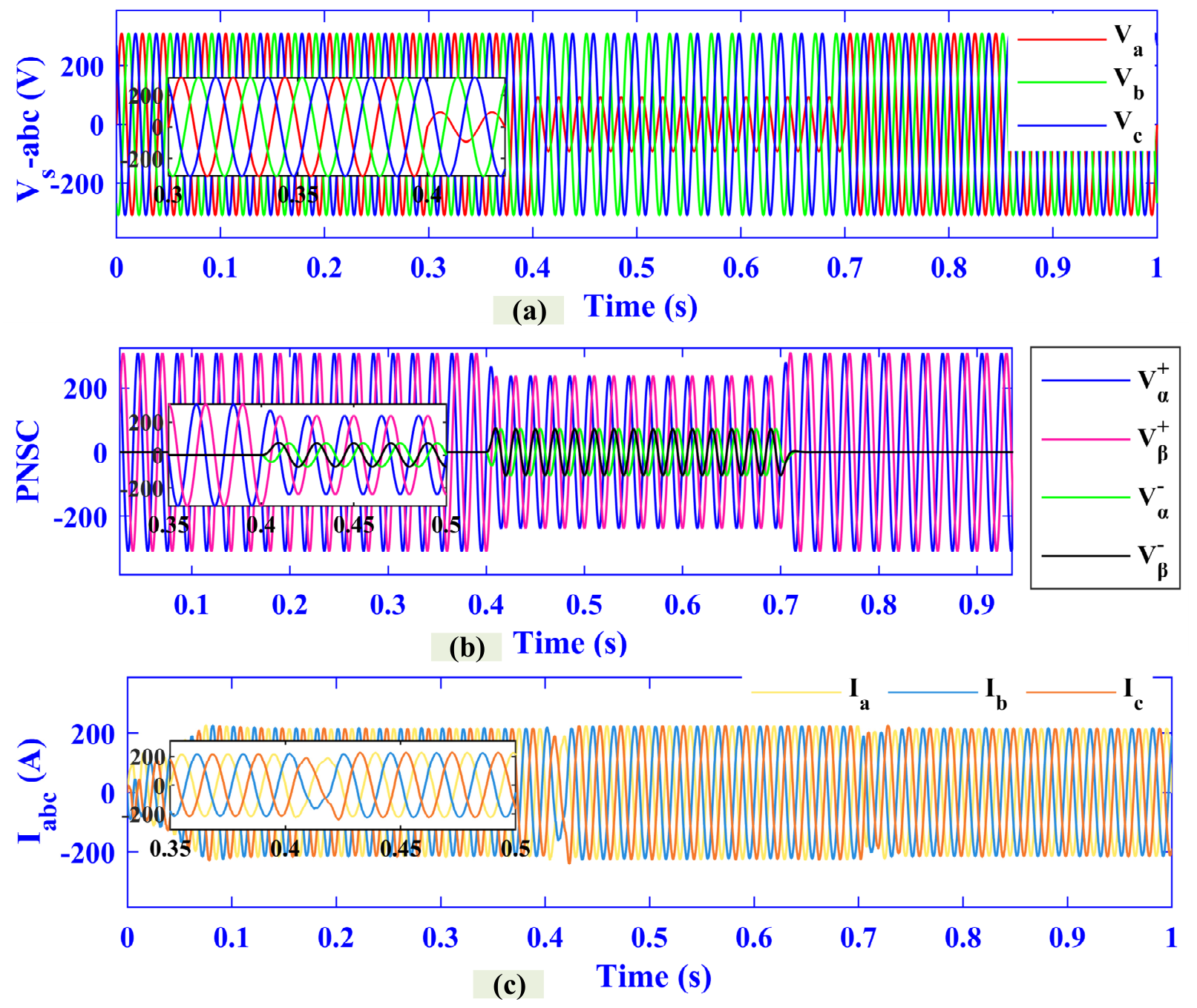
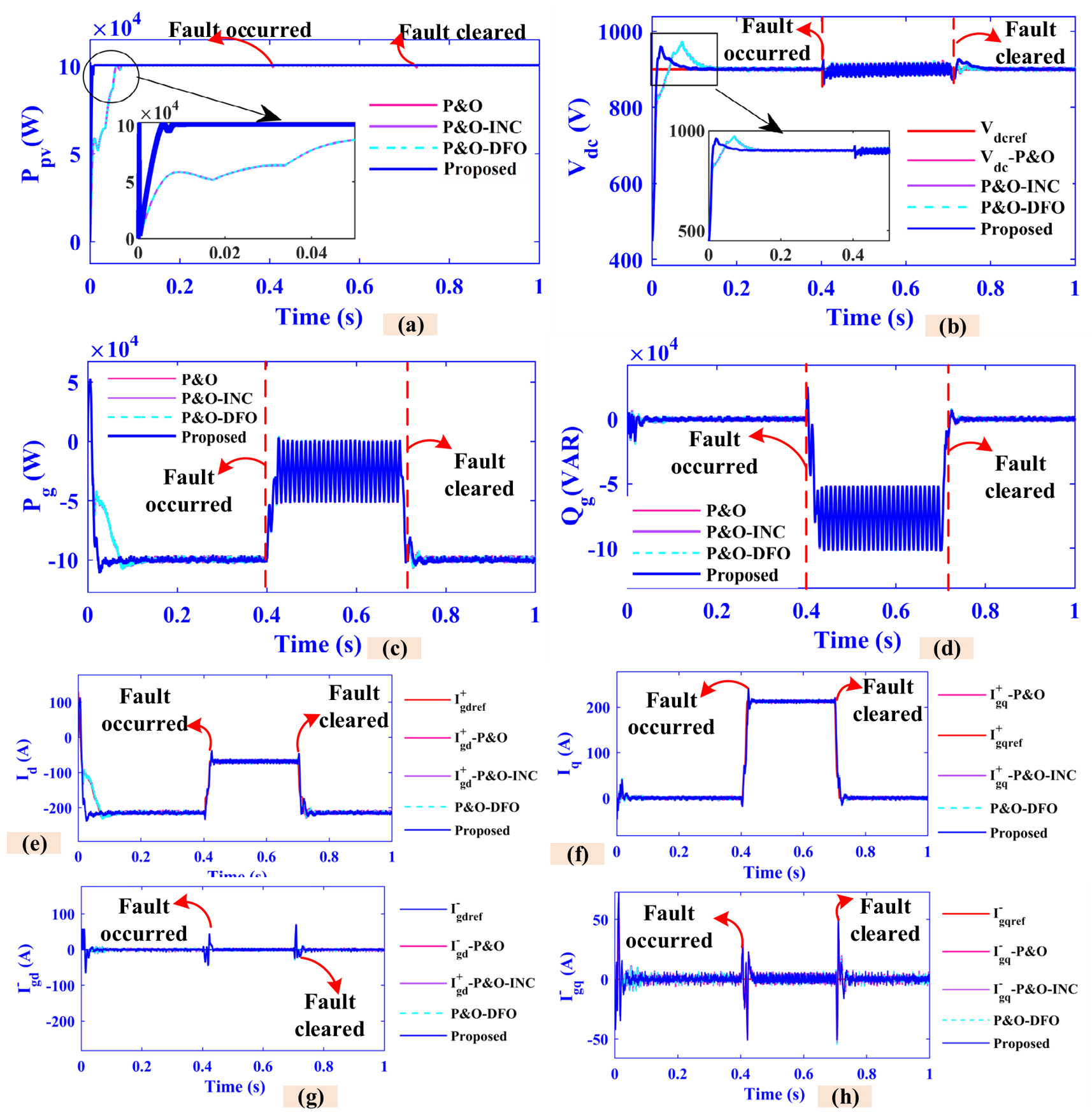
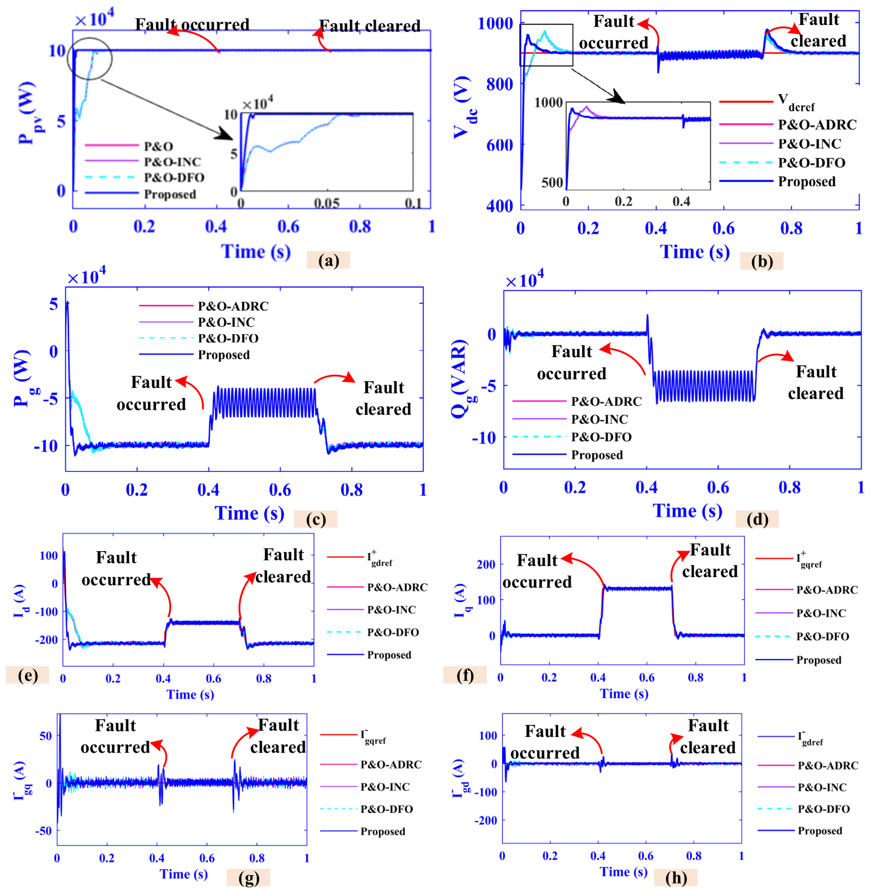
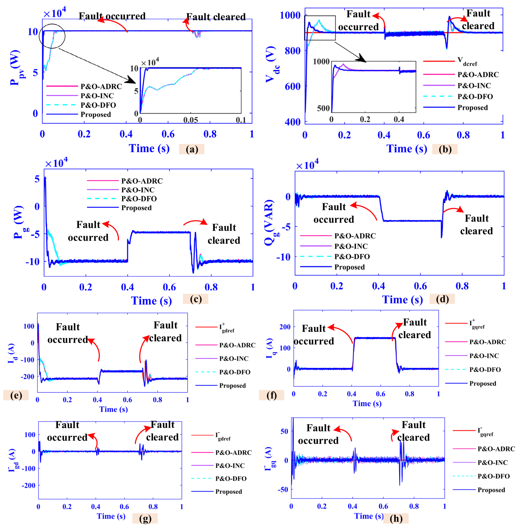
An imbalanced SLG failure that causes the impacted phase voltage on PCC to decrease to 30% in 300 ms is shown in Figure 14. The SLG fault with voltages of 0.3 pu arises from 0.4 s to 0.7 s, as illustrated in Figure 9. The PV provides 10 × 10⁴ W of power from 0 to 1 s and keeps providing this value even during the fault from 0.4 s to 0.7 s; the DC-link voltage is also kept at 900 V. The grid receives 10 × 10⁴ W of actual power between 0 and 0.4 s, which decreases to 6 × 10⁴ W at 0.4 s and stays at 10 × 10⁴ W after 0.7 s. At 0.4 s, the grid’s reactive power is zero, and at 0.7 s, it receives 10 × 10⁴ VAR before falling to zero. Positive and negative current management, along with LVRT capability control, ensures that the inverter output current is consistently kept at a peak current without going above its current limit.

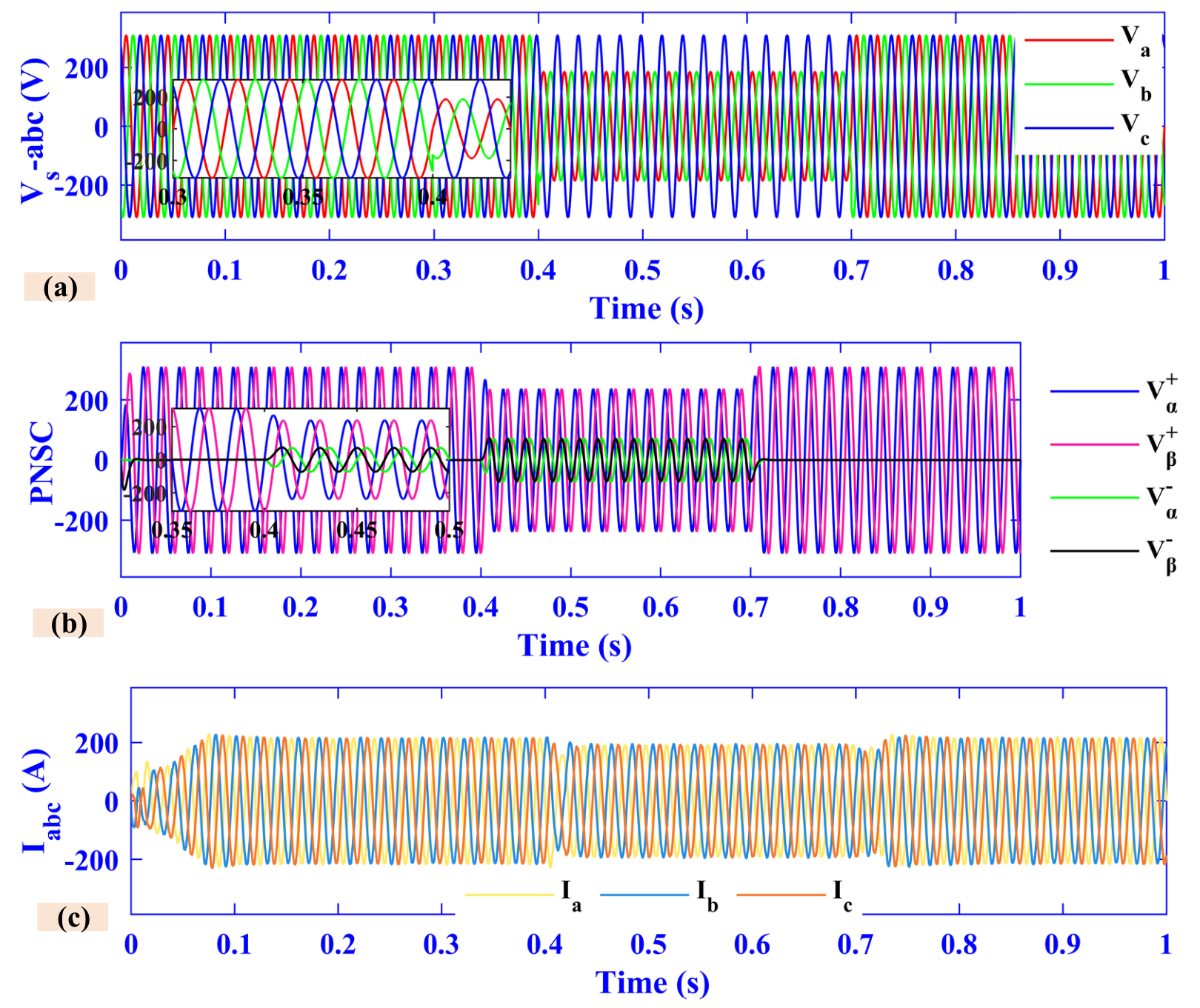
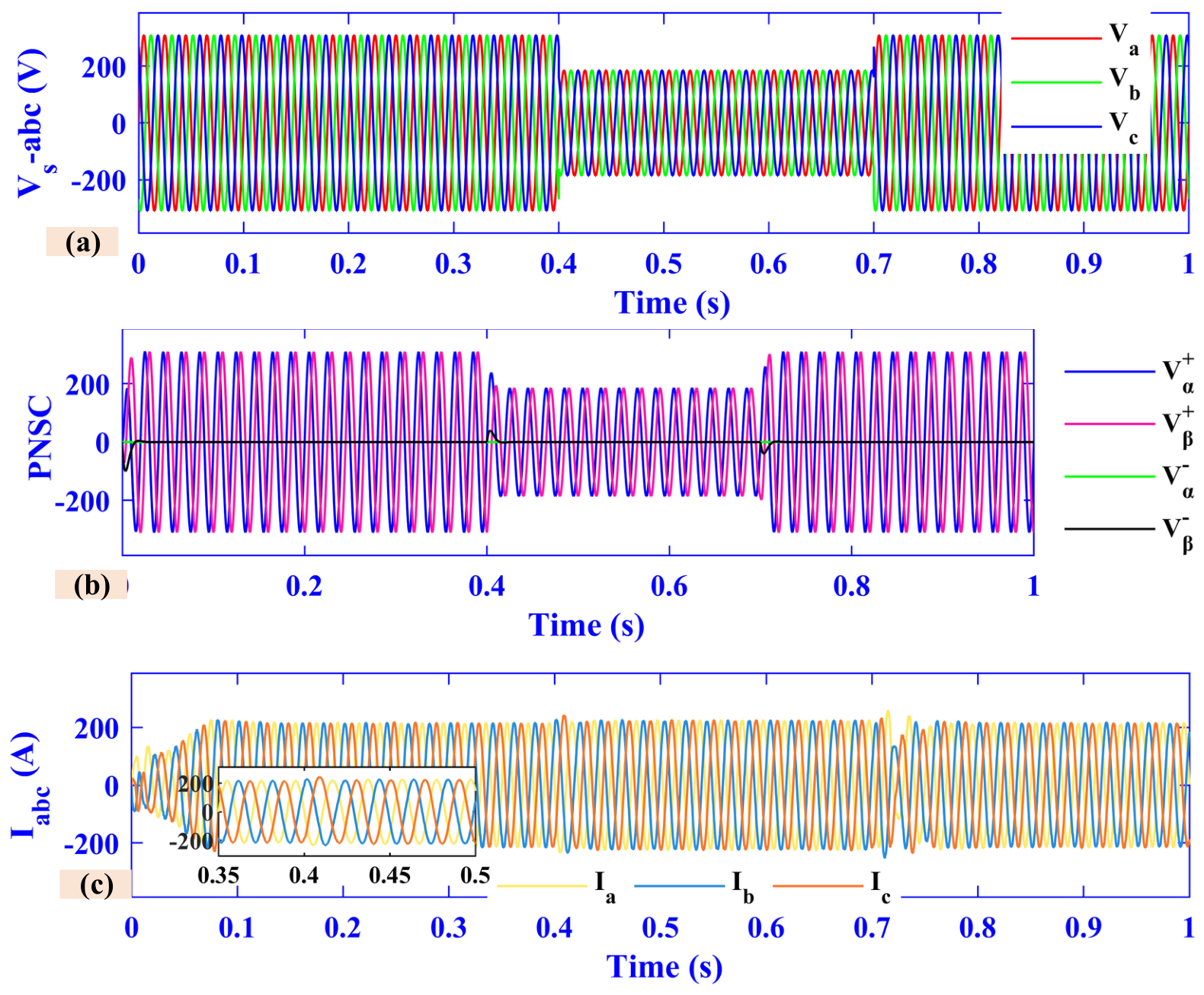
Figure 14 compares the dynamic responses of different MPPT methods during an SLG fault, including PV power, DC-link voltage, grid power, reactive power, and inverter currents. The proposed GPOA-P&O with LADRC demonstrates higher robustness than conventional P&O-based approaches, delivering faster power restoration, lower DC-link voltage overshoot, better reactive power control, and safer current behavior. As illustrated in Figure 15, the inverter voltages, PCC voltages, and output currents remain well-regulated during both fault and recovery periods. The combined use of GPOA-P&O, LADRC, and DSOGI-FLL enables accurate sequence extraction, stable waveform regulation, rapid voltage recovery, and reduced current distortion, confirming the strong LVRT capability of the proposed system.

6.2. Case 02: SLG Fault and Nonuniform PV Radiation with Voltage Sag of 0.3 pu

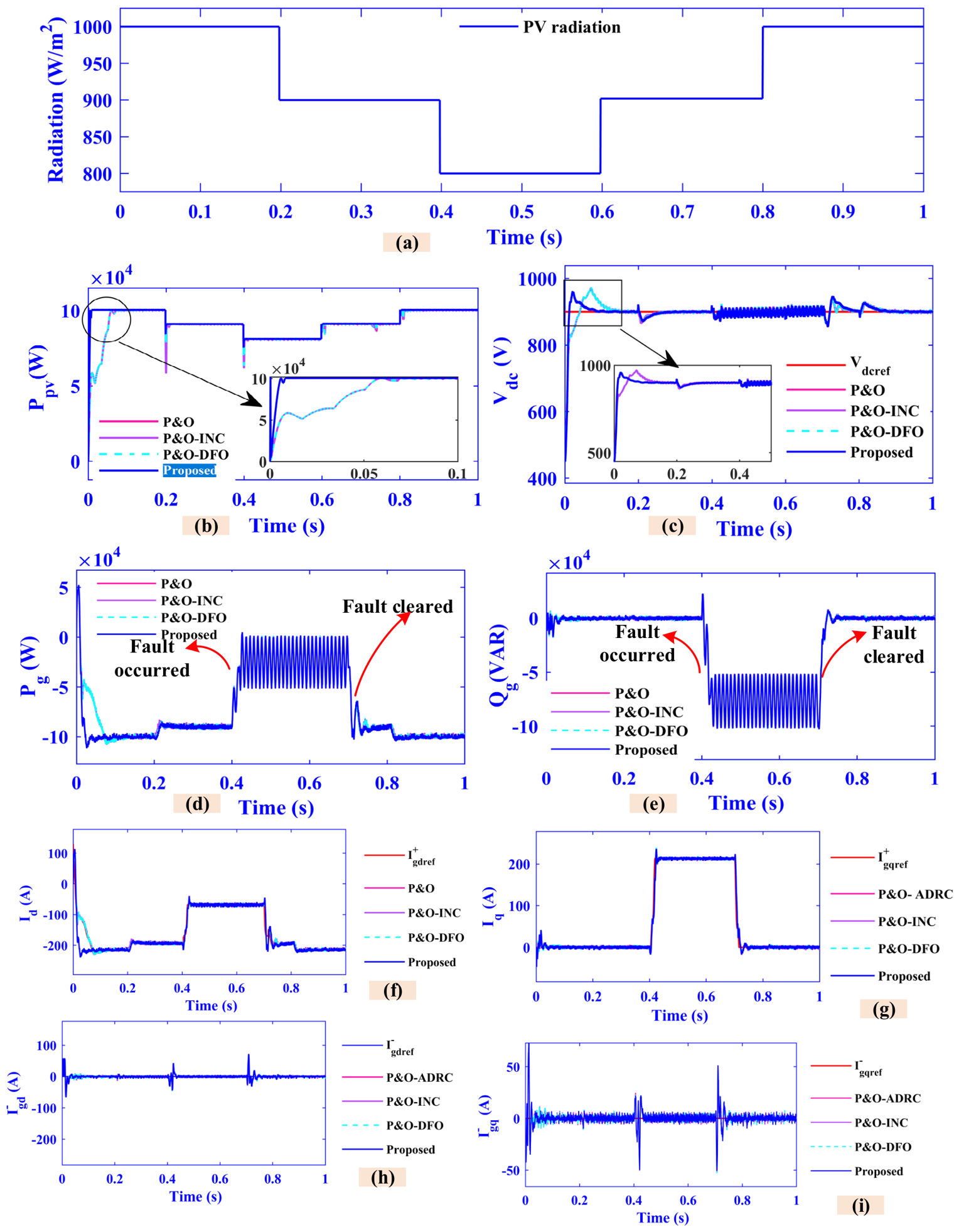
As shown in Figure 16 and Figure 17, during nonuniform PV irradiance and an SLG fault with a 0.3 pu voltage sag, the proposed GPOA-P&O MPPT with ESF, LADRC, and DSOGI-FLL demonstrates strong robustness and fast dynamic response. The proposed control strategy rapidly distinguishes between positive and negative voltage sequences within 2–3 ms, ensuring stable active and reactive power control even under severe grid disturbances. The DC-link voltage deviation is limited to less than 15 V, peaking at 14.2 V during the fault, while the PV output power (P_pv) remains close to its maximum value of 5.0 kW with minimal oscillations of approximately ±2%. The injected current maintains a THD below 3%, significantly outperforming conventional PI-based methods that show THD levels around 7–8% under similar conditions. Following fault clearance, the system restores full power delivery within ~0.04 s, with the DC-link voltage and PV power returning to nominal values without overshoot. These results indicate that the proposed method provides superior LVRT capability, maintaining both transient stability and high-quality steady-state operation under unbalanced and disturbed grid conditions.

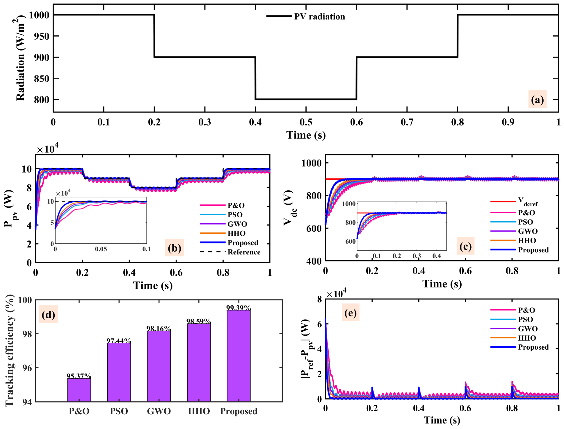
Figure 18 compares the MPPT performance of different algorithms under the same step-changing irradiance profile. As the radiation changes from 1000 to 900, 800, 900, and back to 1000 W/m², all methods attempt to track the corresponding PV maximum power point. Compared to conventional P&O and recent global MPPT methods such as PSO, GWO, and HHO, the proposed GPOA-P&O method shows faster convergence, smaller power oscillation, and better tracking accuracy. The DC-link voltage response also remains closer to its reference value with reduced overshoot and fluctuation, confirming the effectiveness of the proposed method in improving power stability under partial shading and irradiance variation. The proposed GPOA-P&O method achieves faster convergence, higher tracking efficiency, lower power error, reduced power fluctuation, and improved DC-link voltage stability compared to the other MPPT algorithms.

6.3. Two Lines to Ground (2LG) Fault STC and PV Radiation with Voltage Sag of 0.5 pu

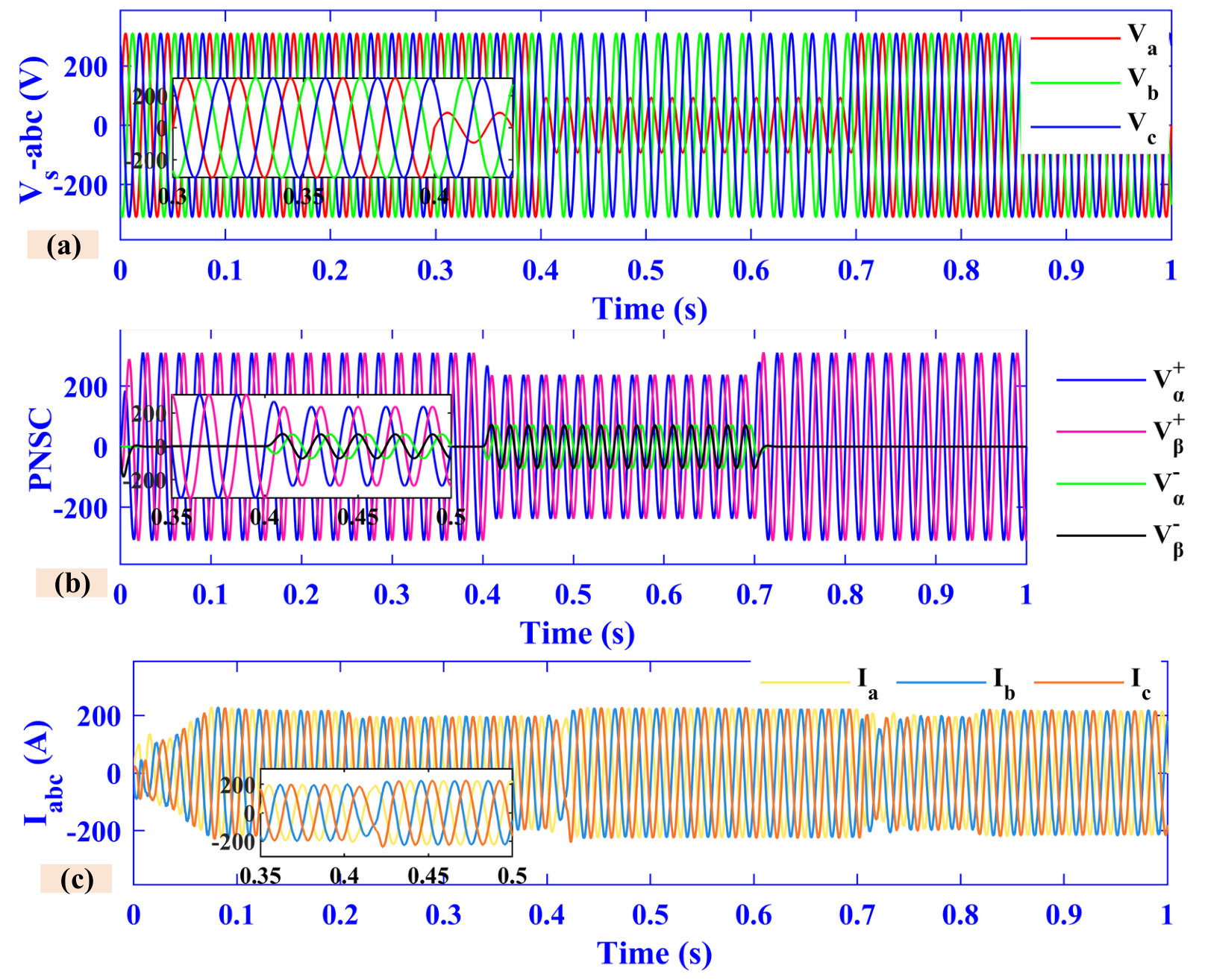
As illustrated in Figure 19 and Figure 20, a two-line-to-ground (2LG) fault accompanied by a 0.5 pu voltage sag arises between 0.4 s and 0.7 s. During normal operation from 0 to 0.4 s, the PV array generates 100 kW of power, which drops to 60 kW immediately at the onset of the fault (0.4 s) before recovering to 100 kW at 0.7 s. Throughout this period, the DC-link voltage remains stable around 900 V, indicating effective voltage regulation under disturbance.

Before the fault, the grid absorbs 100 kW active power, which drops to 60 kW during the fault and recovers to 100 kW after clearance. Reactive power is 0 kVAR in normal operation, rises to 100 kVAR at fault initiation, and returns to 0 kVAR after fault clearance. Owing to the proposed LVRT strategy with positive/negative-sequence current regulation, the inverter output current is held at its allowable peak without exceeding rated limits. The system returns to nominal operation within 100 ms after fault clearance, confirming strong disturbance ride-through, effective voltage support via controlled reactive power injection, and stable current regulation for continuous PV power delivery.

Table 5. Performance assessment of the proposed LVRT control method under 1LG and 2LG fault conditions.

Fault Type	Fault Duration (s)	PV Power (kW)	DC-Link Voltage (V)	Grid Real Power (kW)	Grid Reactive Power (kVAR)	Current THD (%)	Recovery Time (s)
1LG, 0.3 pu sag	0.0–0.3	50 → 50 ± 2%	900 ± 15	100 → 100 ± 2%	0 → 0	<3	~0.04
2LG, 0.5 pu sag	0.4–0.7	100 → 60 → 100	~900	100 → 60 → 100	0 → 100 → 0	<3	<0.1

further summarizes the SLG and 2LG results: under an SLG fault with a 0.3 pu sag, PV power stays near its maximum (50 kW) with ±2% oscillation, the DC-link voltage deviation is limited to 15 V, real power delivery remains nearly constant (~100 kW) with negligible reactive injection, current THD stays below 3%, and full power is restored within ~0.04 s.

During the 2LG fault with a 0.5 pu voltage sag, the PV power drops from 100 kW to 60 kW during the fault and recovers to 100 kW after fault clearance. The DC-link voltage remains stable around 900 V. Grid real power follows a similar trend, while reactive power temporarily rises to 100 kVAR to support voltage recovery. The inverter current remains within safe limits, maintaining THD below 3%. The system returns to normal operation in less than 0.1 s following fault clearance.

6.4. Three Lines to Ground (3LG) Fault and STC PV Radiation with Voltage Sag of 0.6 pu

Figure 21 and Figure 22 illustrate the enhanced performance of the proposed control strategy during an SLG fault. The PV power with the proposed method shows minimal deviation, maintaining an average of 100 kW during the fault, compared to a significant drop in conventional methods. The DC-link voltage is effectively regulated, peaking at only 900 V and stabilizing rapidly. The grid power demonstrates a controlled reduction to 50 kW during the fault, ensuring continuous active power injection as per LVRT requirements. Simultaneously, the reactive power swiftly increases to 50 kVAR to support grid-voltage recovery. The inverter currents exhibit balanced and stable waveforms with minimal distortion, underscoring the robustness of ADRC and DSOGI-FLL in maintaining synchronization and control during the fault. Overall, the proposed method ensures superior LVRT compliance and system stability.

The proposed GPOA-P&O with ESF reduces power fluctuations by bypassing local peaks and tracking the global maximum power point. Meanwhile, the cascaded LADRC loops regulate voltage and current accurately to suppress DC-link overvoltage. The DSOGI-FLL provides precise phase synchronization under unbalanced voltage conditions, enabling compliant reactive current injection. As a result, the integrated control scheme improves LVRT capability and enhances grid support during faults.

6.5. Discussions

As shown in Figure 14 and Figure 15, the system operates under global maximum power harvesting and unity power factor prior to fault occurrence, with all PV power delivered to the grid and reactive power regulated to zero. During the fault, the DSOGI-FLL accurately separates positive and negative voltage sequences, providing reliable control references. Active power injection is appropriately limited, while ADRC regulates the positive-sequence current to its reference and suppresses the negative-sequence current to zero. The grid currents remain within nominal limits, and the DC-link voltage is effectively stabilized.

When a fault occurs, excess power causes a temporary DC-link voltage rise. The ADRC adjusts the d-axis current reference to mitigate this effect, while a discharge circuit dissipates surplus energy once the voltage exceeds a threshold, preventing double-line-frequency oscillations.

Figure 19 and Figure 20 present the response under an unbalanced 2LG fault (50% voltage sag for 300 ms), demonstrating secure inverter operation and compliance with grid-code requirements through proper reactive power support. Figure 21 and Figure 22 show a balanced three-phase fault (60% sag), where the system recovers to pre-fault conditions within 100 ms after clearance.

Overall, the results confirm that the proposed LVRT control strategy effectively withstands various fault types, supports voltage recovery via controlled reactive power injection, and maintains stable system operation.

6.6. Comparative Analysis

Table 6. Dynamic response characteristics of key PV system parameters under fault conditions.

Subplot	Parameters	Values
Grid Voltage	Settling time	0.07
	Overshoot	5%
	Undershoot	5%
	Steady-state error	0
PNSC Extraction	Settling time	0.08
	Overshoot	6%
	Undershoot	8%
	Steady-state error	0
PV power	Settling time	0.1
	Overshoot	10%
	Undershoot	0
	Steady-state error	0
Active Power	Settling time	0.12
	Overshoot	5%
	Undershoot	20%
	Steady-state error	0
DC-Link Voltage	Settling time	0.05
	Overshoot	2%
	Undershoot	5%
	Steady-state error	0

summarizes the transient response of the proposed GPOA-P&O MPPT with ESF, LADRC, and DSOGI-FLL control strategy for key system variables, including grid voltage, PNSC extraction, PV power, active power, and DC-link voltage. The integrated approach achieves fast dynamic response, with settling times as low as 0.05 s for DC-link voltage regulation and 0.07–0.12 s for other parameters. Overshoot remains modest, peaking at 10% for PV power, while undershoot is minimized, except for active power (20%). Crucially, the steady-state error is zero for all measured outputs, showing that the proposed method not only enhances LVRT stability but also delivers precise final tracking under grid disturbances. In addition, Table 6 summarizes the transient performance of key PV system parameters under disturbances. All variables exhibit fast settling times (0.05–0.12 s), low overshoot and undershoot, and zero steady-state error, demonstrating the proposed control strategy’s ability to maintain stable voltage, accurate power tracking, and robust DC-link regulation during dynamic events.

Table 7. Comparison of PV system fault-response methods.

Feature	Proposed Method	Ref. [8]	Ref. [6]
Connection	Two-stage PV system using GPOA-P&O with ESF, LADRC, and DSOGI-FLL	Double-stage	Single-stage
Energy dissipation	ADRC clamps DC-link	None	Resistive discharge required
Efficiency	>99% (simulation)	High	Lower (power dissipated)
Complexity	Moderate control structure	Very simple	High
Fault response	Smooth power, <5% overshoot, <0.1 s settling	Smooth response	Large oscillations
PV Operational Point	Temporarily moves from MPP during LVRT	Moves away from MPP	Always at MPP
DC-link voltage	Within ±10% of nominal	Up to +20%	Nearly constant

compares the proposed two-stage PV control strategy, GPOA-P&O with ESF, LADRC, and DSOGI-FLL, with two existing methods in terms of grid connection type, energy dissipation, efficiency, control complexity, fault response, operating-point behavior, and DC-link voltage performance. The proposed method offers high efficiency (>99%), precise MPPT, minimal oscillations, smooth active/reactive power control, and tight DC-link voltage regulation. In contrast, the method from Ref. [6] is simpler but less adaptive to voltage regulation, while the method from Paper [8] suffers from higher oscillations and requires bulkier hardware for fault energy dissipation.

6.7. Validation of Performance in a Real-Time Setting

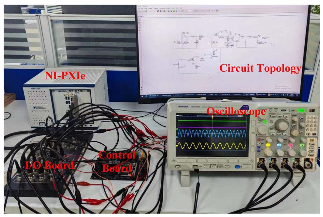
The HIL validation was carried out using an NI PXIe-based real-time platform as shown in Figure 23. It should be clarified that the NI PXIe-1071 is the PXIe chassis used to host the real-time hardware modules, rather than the simulator itself. The real-time simulation model was implemented on the PXIe real-time/FPGA target, while the proposed control algorithm was executed through the DSP 180 interface board. The HIL model includes the PV array, DC–DC boost converter, DC-link capacitor, grid-connected inverter, grid-side filter, grid source, and fault-generation module. The exchanged signals include measured PV voltage/current, DC-link voltage, grid voltage/current, PWM/gating signals, and fault-control commands. The controller sampling period was set to 50 µs, and the inverter switching frequency was set to 10 kHz. The DSP 180 board was used as the controller interface for signal acquisition, PWM generation, and communication with the real-time HIL platform. The hardware configuration, real-time model, and signal-flow structure have been added to improve reproducibility.

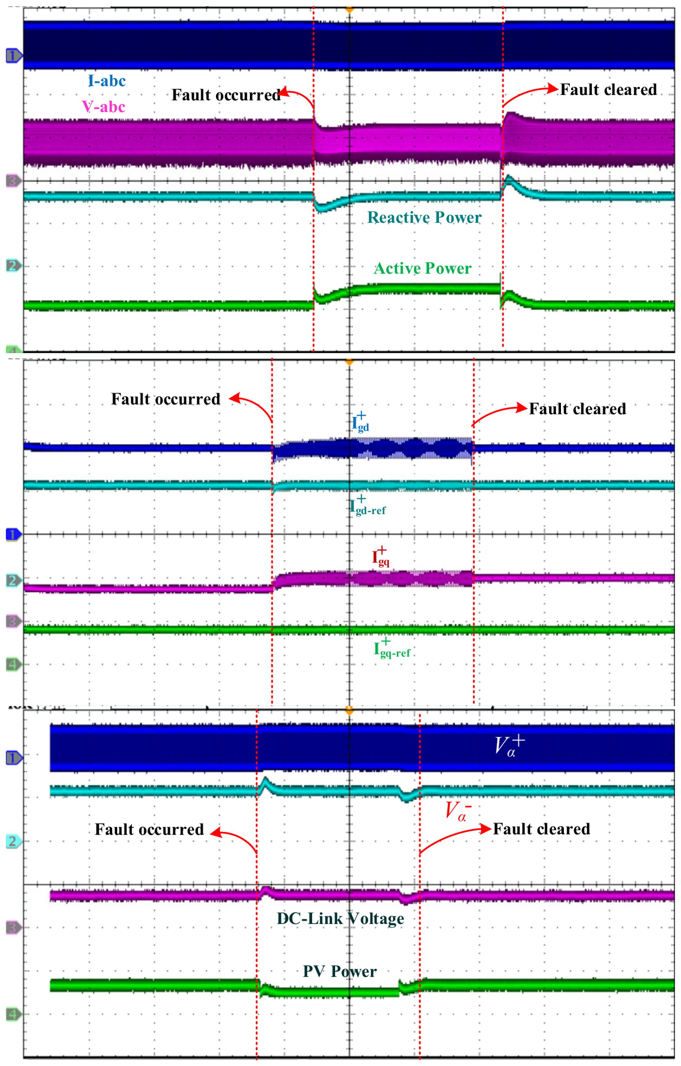
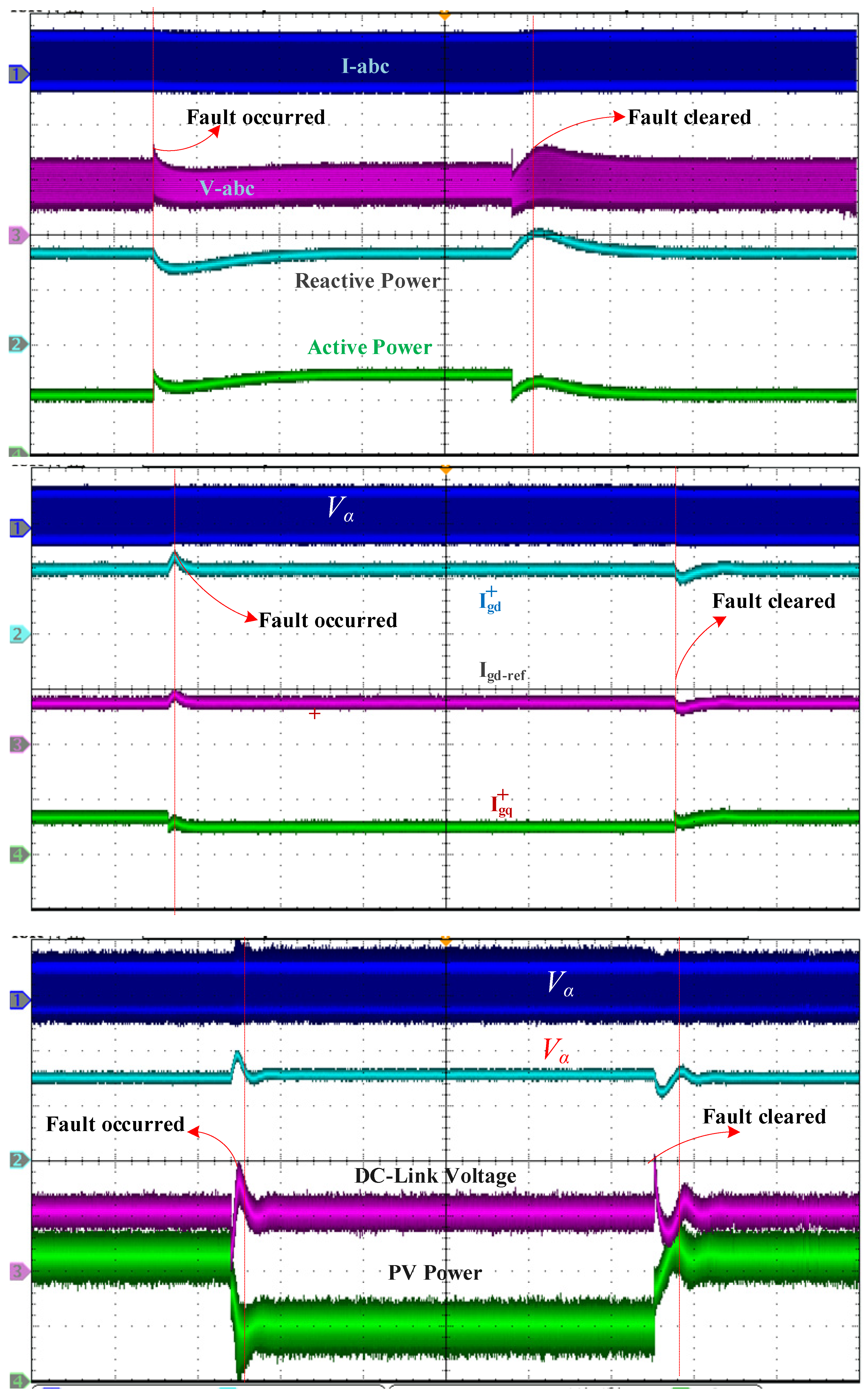
Figure 24 shows the HIL verification of the proposed two-stage PV system, integrating GPOA-P&O MPPT with LADRC–DSOGI-FLL control, under grid-fault conditions. Grid currents I_abc, voltages V_abc, and active/reactive power show only minor transients and smooth recovery after fault clearance. The current components I_gd and I_gq accurately track their references with minimal oscillations, confirming precise current regulation. Positive- and negative-sequence voltages, DC-link voltage, and PV power indicate temporary disturbances during the fault but rapid stabilization afterward. These results demonstrate the robustness, fast dynamic response, and strong fault ride-through capability of the proposed control strategy. Figure 25 shows the NI PXIE-1071 HIL results for Case Two. The I_abc and V_abc waveforms exhibit disturbances during the fault and recover after clearance, with corresponding variations in active and reactive power. The DC-link voltage and PV power also experience temporary disturbances but quickly return to steady operation, confirming the system’s stability and resilience under fault conditions.

The switching frequency was selected as 10 kHz to provide a practical compromise between current-ripple reduction, switching loss, and real-time computational burden. The corresponding switching period is 100 µs. In this study, the control sampling period was set to 50 µs, corresponding to a sampling frequency of 20 kHz. Therefore, the digital controller is updated at twice the switching frequency, which provides sufficient resolution for the voltage and current control loops while satisfying the real-time execution requirement of the HIL platform. The effect of discretization was also considered in the LADRC bandwidth selection. The largest observer bandwidth used in this work is 1200 rad/s, which is approximately 191 Hz, while the sampling frequency is 20 kHz. Hence, the sampling frequency is more than 100 times higher than the maximum observer bandwidth. This large separation limits discretization-induced phase delay and helps maintain the stability margin of the LADRC controllers. The simulation and HIL results further confirm that the selected sampling period does not cause noticeable instability, excessive overshoot, or degradation of LVRT recovery performance.

The numerical comparison in

Table 8. Quantitative comparison between simulation and HIL results under 2LG fault condition.

Performance Indicator	Simulation Result	HIL Result	Difference/Deviation	Comment
Fault condition	2LG, 0.5 pu sag	2LG, 0.5 pu sag	—	Same fault condition
Fault duration	0.4–0.7 s	0.4–0.7 s	—	Same test interval
PV power during fault	100 → 60 → 100 kW	100 → 60 → 100 kW	Very small	HIL follows simulation trend
DC-link voltage	~900 V/900 ± 15 V	~900 V/900 ± 15 V	Within ±15 V	Stable DC-link regulation
Grid real power	100 → 60 → 100 kW	100 → 60 → 100 kW	Very small	Active power tracks fault condition
Grid reactive power	0 → 100 → 0 kVAR	0 → ~100 → 0 kVAR	Very small	Reactive current support is achieved
Current THD	<3%	≤3%	Negligible	Satisfies power-quality requirement
Recovery time	<0.1 s	0.08–0.10 s	Close agreement	HIL validates real-time feasibility
DC-link settling time	0.05 s	approximately 0.08–0.10 s	Slightly higher in HIL	Due to real-time delay and hardware interface
DC-link overshoot	2%	within ±15 V around 900 V	Acceptable	Overvoltage is effectively suppressed
Steady-state error	0	approximately 0	Negligible	Stable post-fault recovery

shows that the HIL results are highly consistent with the simulation results under the same 2LG fault condition. Small differences in recovery time and transient voltage fluctuation are expected because the HIL platform includes real-time sampling, discretization, and hardware interface delays, but the proposed controller still maintains stable DC-link voltage, current THD below 3%, effective reactive power injection, and fast post-fault recovery.

Figure 26 shows that the proposed GPOA-P&O with ESF, LADRC, and DSOGI-FLL strategy provides better DC-link voltage regulation, lower THD, smoother power tracking, and stronger reactive power support than conventional PI control during pre-fault, fault, and post-fault operation.

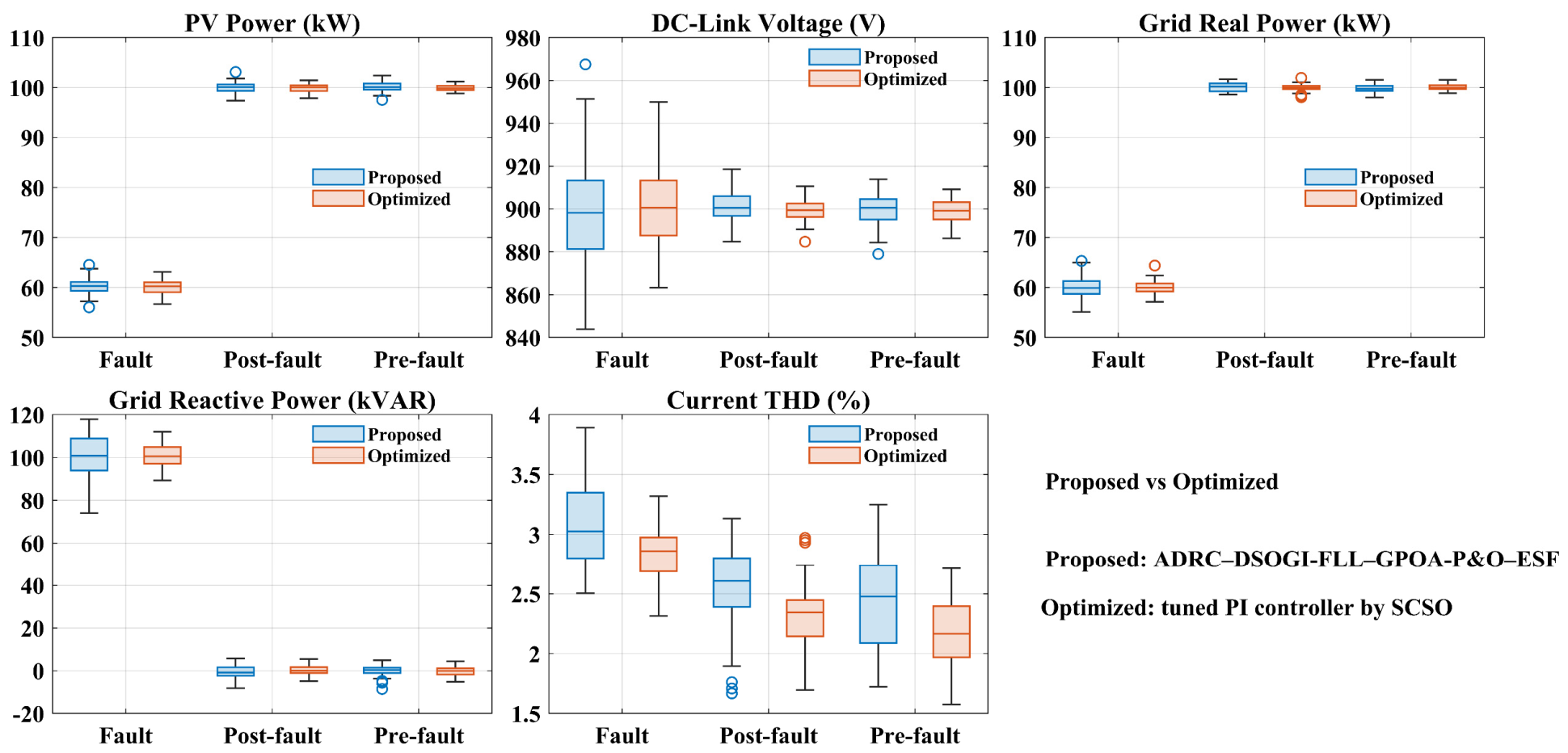
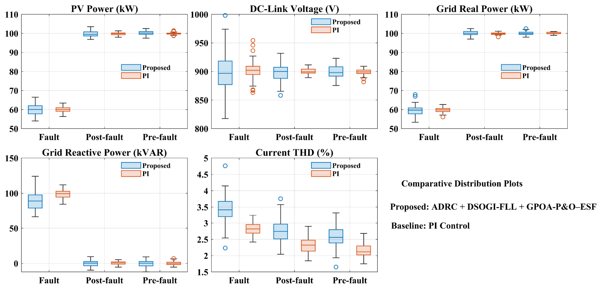
Figure 27 compares the distribution of key performance indicators, including PV power, DC-link voltage, grid power, reactive power, and THD, during pre-fault, fault, and post-fault operation. The results show that the proposed GPOA-P&O–ESF–LADRC–DSOGI-FLL control strategy provides more accurate regulation, lower distortion, and stronger fault ride-through capability than the Sand Cat Swarm Optimization SCSO-tuned PI controller.

It should be noted that the efficiency value reported in this study mainly refers to the MPPT tracking efficiency, rather than the total power-conversion efficiency of the complete PV converter system. In practical implementation, several non-ideal factors may influence the overall system performance. Converter conduction and switching losses can slightly reduce the delivered grid power and decrease the net conversion efficiency. Sensor noise in voltage and current measurements may introduce small fluctuations in the MPPT process, DC-link voltage regulation, and current control loops. Parameter uncertainties, such as variations in filter inductance, DC-link capacitance, line impedance, and PV module parameters, can affect settling time, overshoot, and steady-state ripple. In addition, aging effects of PV modules, capacitors, and semiconductor devices may gradually reduce the available PV power and increase thermal and dynamic stress. Although these non-idealities were not the primary focus of the present work, the LADRC structure is expected to improve robustness by estimating and compensating lumped disturbances through the extended state observer, while DSOGI-FLL provides filtering and synchronization capability under distorted grid conditions. Future work will further investigate the proposed strategy under detailed converter-loss models, sensor noise, parameter mismatch, and long-term aging conditions.

Although the present study focuses on SLG, 2LG, and 3LG voltage-sag conditions, the proposed coordinated control strategy is also expected to provide stable performance under other practical grid disturbances. For line-to-line faults, which are asymmetrical disturbances, negative-sequence voltage components are generated; therefore, the DSOGI-FLL block can be used to extract the positive- and negative-sequence components and maintain accurate synchronization for reactive current support. Under frequency deviations, the FLL mechanism adaptively tracks the grid angular frequency, allowing the controller to maintain phase-locking accuracy when the frequency varies around its nominal value. In the presence of grid-voltage harmonics, the SOGI structure provides inherent filtering capability, while LADRC can compensate part of the resulting disturbance through the extended state observer. Nevertheless, severe harmonic distortion, large frequency deviations, and combined weak-grid disturbances require further validation. Future work will therefore extend the testing scenarios to line-to-line faults, frequency variations, harmonic distortion, and combined fault–harmonic operating conditions.

7. Conclusions

This paper proposed an enhanced LVRT control strategy for three-phase grid-connected PV systems under symmetrical and asymmetrical grid faults. The proposed framework integrates GPOA-P&O–ESF MPPT, cascaded LADRC control loops, and DSOGI-FLL synchronization to improve global power tracking, DC-link voltage regulation, and grid-support capability during fault conditions. The GPOA-P&O–ESF method reduces power oscillations by avoiding local maximum points and tracking the global MPP, while the LADRC-based voltage and current loops suppress DC-link overvoltage within 5% of its nominal value. In addition, the DSOGI-FLL provides accurate positive-sequence phase tracking with a phase error below 0.5°, enabling compliant reactive current injection even under 40% voltage asymmetry.

The MATLAB/Simulink results confirm that the proposed GPOA-P&O–ESF–LADRC–DSOGI-FLL strategy delivers superior dynamic performance compared to the conventional PI–PLL approach. It achieves a 35% reduction in post-fault settling time, limits overshoot to below 6%, and maintains 100% LVRT success across all tested fault scenarios. These results demonstrate the strong robustness, fast transient response, and improved grid-code compliance of the proposed method.

In addition to the LVRT control methods summarized in the manuscript, advanced nonlinear and learning-based controllers, such as state-filtered disturbance-rejection control and multilayer neuroadaptive reinforcement-learning control based on actor–critic mechanisms, have recently been applied to disturbed nonlinear systems. These methods offer strong adaptability and disturbance-rejection capability, especially when system dynamics are highly uncertain. However, their application to grid-connected PV LVRT control generally requires additional state filtering, training or online learning mechanisms, higher computational effort, and rigorous stability verification. In contrast, the proposed strategy adopts a physically coordinated structure in which GPOA-P&O improves global MPPT tracking under partial shading, LADRC enhances DC-link voltage and current regulation during grid faults, and DSOGI-FLL ensures accurate synchronization and sequence extraction under unbalanced disturbances. Therefore, the proposed method provides a practical balance between robustness, implementation simplicity, and LVRT performance. Future work will further compare the proposed framework with advanced state-filtered disturbance rejection and actor–critic neuroadaptive control methods under broader grid disturbances and hardware conditions.

References

1. Ozgenc, B.; Aslanhan, Y.A.B.; Altas, I.H. Improving LVRT Capability in Grid Connected PV System Using DRL Based Controller. IEEE Access 2025, 13, 41025–41039. [Google Scholar] [CrossRef]
2. Almesri, Z.M.; Hussain, H.A.; Kamel, R.M. Low Voltage Ride-through Capability of Grid-Connected PV Systems: A Comparative Study of Grid-Following and Grid-Forming Converters under Current Limits. IEEE Access 2025, 13, 105590–105607. [Google Scholar] [CrossRef]
3. Sakthivel, T.S.; Ragupathy, P.; Chinnadurai, N. Adaptive Sliding Mode Control of Multilevel Grid-Connected Inverters Using Reinforcement Learning for Enhanced LVRT Performance. Electr. Power Syst. Res. 2026, 253, 112428. [Google Scholar] [CrossRef]
4. Li, B.; Wang, Y. Enhanced Low-Voltage Ride-through Scheme for Grid-Forming Converters Considering Current Limitation and Transient Stability Simultaneously. Sustainability 2025, 17, 1428. [Google Scholar] [CrossRef]
5. Rios-Castro, D.; Pérez-Estévez, D.; Doval-Gandoy, J. Grid-Connected Converter with Grid-Forming and Grid-Following Modes Presenting Symmetrical and Asymmetrical Fault Ride-through Capability. IEEE J. Emerg. Sel. Top. Power Electron. 2024, 12, 2082–2096. [Google Scholar] [CrossRef]
6. Basu Roy Chowdhury, S.; Gayen, P.K. An Improved Capability of LVRT in Single-Stage Three-Phase Grid-Linked PV Systems. Electr. Eng. 2024, 106, 125–143. [Google Scholar]
7. Capovilla, C.E.; Casella, I.R.S.; Sguarezi Filho, A.J.; Azcue-Puma, J.L.; Jacomini, R.V.; Ruppert, E. A Wind Energy Generator for Smart Grid Applications Using Wireless-Coded Neuro-Fuzzy Power Control. Comput. Math. Appl. 2014, 68, 2112–2123. [Google Scholar] [CrossRef]
8. Aboudrar, I.; El Hani, S.; Mediouni, H.; Naseri, N.; Daghouri, A. LVRT Capability Enhancement of a Grid Connected Three Phase PV System by ADRC and DSOGI FLL. Int. Trans. Electr. Energy Syst. 2021, 31, e13059. [Google Scholar] [CrossRef]
9. Al-Shetwi, A.Q.; Sujod, M.Z.; Blaabjerg, F. Low Voltage Ride-through Capability Control for Single-Stage Inverter-Based Grid-Connected Photovoltaic Power Plant. Sol. Energy 2018, 159, 665–681. [Google Scholar] [CrossRef]
10. Lin, F.-J.; Lu, K.-C.; Ke, T.-H.; Yang, B.-H.; Chang, Y.-R. Reactive Power Control of Three-Phase Grid-Connected PV System during Grid Faults Using Takagi–Sugeno–Kang Probabilistic Fuzzy Neural Network Control. IEEE Trans. Ind. Electron. 2015, 62, 5516–5528. [Google Scholar] [CrossRef]
11. Hamrouni, N.; Jraidi, M.; Ghobber, A.; Dhouib, A. Control Approach of a Connected PV System under Grid Faults. Electr. Eng. 2018, 100, 1205–1217. [Google Scholar]
12. Hasanien, H.M. An Adaptive Control Strategy for Low Voltage Ride through Capability Enhancement of Grid-Connected Photovoltaic Power Plants. IEEE Trans. Power Syst. 2015, 31, 3230–3237. [Google Scholar]
13. He, W.; Pan, H.; Chen, S.; Li, Z. Active LVRT Strategy Based on Improved Pv Engineering Model and Power Feedforward. In Proceedings of the 2018 Chinese Automation Congress (CAC), Xi’an, China, 30 November–2 December 2018; IEEE: New York, NY, USA, 2018; pp. 2212–2217. [Google Scholar]
14. Liu, H.; Xu, K.; Zhang, Z.; Liu, W.; Ao, J. Research on Theoretical Calculation Methods of Photovoltaic Power Short-Circuit Current and Influencing Factors of Its Fault Characteristics. Energies 2019, 12, 316. [Google Scholar] [CrossRef]
15. Ali, Z.; Christofides, N.; Hadjidemetriou, L.; Kyriakides, E.; Yang, Y.; Blaabjerg, F. Three-Phase Phase-Locked Loop Synchronization Algorithms for Grid-Connected Renewable Energy Systems: A Review. Renew. Sustain. Energy Rev. 2018, 90, 434–452. [Google Scholar] [CrossRef]
16. Huang, X.; Wang, H.; Wang, Y.; Xu, H. Voltage Rise Regulation with Voltage Source Inverter in Grid Connected PV Generation System. In Proceedings of the 2013 International Conference on Electrical Machines and Systems (ICEMS), Busan, Republic of Korea, 26–29 October 2013; IEEE: New York, NY, USA, 2013; pp. 431–434. [Google Scholar]
17. Golestan, S.; Guerrero, J.M.; Vasquez, J.C. Three-Phase PLLs: A Review of Recent Advances. IEEE Trans. Power Electron. 2016, 32, 1894–1907. [Google Scholar]
18. Sorkhabi, S.S.; Bakhshai, A. Microgrid Control Strategies and Synchronization Techniques during Transition between Grid-Connected and Stand-Alone Mode of Operation. In Proceedings of the 2015 IEEE International Telecommunications Energy Conference (INTELEC), Osaka, Japan, 18–22 October 2015; IEEE: New York, NY, USA, 2015; pp. 1–5. [Google Scholar]
19. Khan, H.; Chacko, S.J.; Fernandes, B.G.; Kulkarni, A. An Integrated Controller to Perform LVRT Operation in PV Systems Connected to a LV Grid during Balanced and Unbalanced Faults. In Proceedings of the 2017 IEEE 3rd International Future Energy Electronics Conference and ECCE Asia (IFEEC 2017-ECCE Asia), Kaohsiung, Taiwan, 3–7 June 2017; IEEE: New York, NY, USA, 2017; pp. 2002–2007. [Google Scholar]
20. Lei, H.; Yang, C.; Li, J.; Xie, Y. A LVRT Control Strategy Based on the Improved Second Order Generalized Integral PLL. In Proceedings of the 2017 International Conference on Applied Mathematics, Modeling and Simulation (AMMS 2017), Shanghai, China, 26–27 November 2017; Atlantis Press: Dordrecht, The Netherlands, 2017; pp. 66–69. [Google Scholar]
21. Ren, X.; Lyu, Z.; Li, D.; Zhang, Z.; Zhang, S. Synchronization Signal Extraction Method Based on Enhanced DSSOGI-FLL in Power Grid Distortion. Syst. Sci. Control Eng. 2018, 6, 305–313. [Google Scholar] [CrossRef]
22. Gholipour, A.; Farhadi-Kangarlu, M.; Neyshabouri, Y.; Talavat, V. Low Voltage Ride through (LVRT) Enhancement of a Two-Stage Grid-Connected Photovoltaic System Based on Finite-Control-Set Model Predictive Control Strategy. Int. J. Renew. Energy Dev. 2025, 14, 404–419. [Google Scholar] [CrossRef]
23. Gencer, A. Low Voltage Ride-through Improvement of a Grid-Connected Pv Power System Using a Machine Learning Control System. Appl. Sci. 2025, 15, 4251. [Google Scholar] [CrossRef]
24. Luan, X.; Zhao, G.; Li, W.; Qiao, G.; Sun, H.; Xu, Y. A Low-Voltage Ride-Through Strategy for Two-Stage PV Inverter with DSOGI Phase-Locked Loop. In Proceedings of the 2024 IEEE 7th International Conference on Automation, Electronics and Electrical Engineering (AUTEEE), Shenyang, China, 27–29 December 2024; IEEE: New York, NY, USA, 2024; pp. 555–559. [Google Scholar]
25. Alharbi, Y.; Darwish, A.; Ma, X. A Review of Model Predictive Control for Grid-Connected PV Applications. Electronics 2025, 14, 667. [Google Scholar] [CrossRef]
26. Praiselin, W.J.; Edward, J.B. Voltage Profile Improvement of Solar PV Grid–Connected Inverter with Micro Grid Operation Using PI Controller. Energy Procedia 2017, 117, 104–111. [Google Scholar] [CrossRef]
27. Han, J. From PID to Active Disturbance Rejection Control. IEEE Trans. Ind. Electron. 2009, 56, 900–906. [Google Scholar] [CrossRef]
28. Feng, H.; Guo, B.-Z. Active Disturbance Rejection Control: Old and New Results. Annu. Rev. Control 2017, 44, 238–248. [Google Scholar] [CrossRef]
29. Kalyan, N.S.; Sambasiva Rao, G. Frequency and Voltage Stabilisation in Combined Load Frequency Control and Automatic Voltage Regulation of Multiarea System with Hybrid Generation Utilities by AC/DC Links. Int. J. Sustain. Energy 2020, 39, 1009–1029. [Google Scholar] [CrossRef]
30. Shah, R.; Mithulananthan, N.; Bansal, R.C.; Ramachandaramurthy, V.K. A Review of Key Power System Stability Challenges for Large-Scale PV Integration. Renew. Sustain. Energy Rev. 2015, 41, 1423–1436. [Google Scholar] [CrossRef]
31. Cabrera-Tobar, A.; Bullich-Massagué, E.; Aragüés-Peñalba, M.; Gomis-Bellmunt, O. Review of Advanced Grid Requirements for the Integration of Large Scale Photovoltaic Power Plants in the Transmission System. Renew. Sustain. Energy Rev. 2016, 62, 971–987. [Google Scholar] [CrossRef]
32. Mansouri, N.; Lashab, A.; Sera, D.; Guerrero, J.M.; Cherif, A. Large Photovoltaic Power Plants Integration: A Review of Challenges and Solutions. Energies 2019, 12, 3798. [Google Scholar] [CrossRef]
33. Yau, H.-T.; Liang, Q.-C.; Hsieh, C.-T. Maximum Power Point Tracking and Optimal Li-Ion Battery Charging Control for Photovoltaic Charging System. Comput. Math. Appl. 2012, 64, 822–832. [Google Scholar] [CrossRef][Green Version]
34. Benmessaoud, M.T.; Zerhouni, F.Z.; Zegrar, M.; Stambouli, A.B.; Tioursi, M. New Approach Modeling and a Maximum Power Point Tracker Method for Solar Cells. Comput. Math. Appl. 2010, 60, 1124–1134. [Google Scholar] [CrossRef]
35. Al-Wesabi, I.; Fang, Z.; Hussein Farh, H.M.; Al-Shamma’a, A.A.; Al-Shaalan, A.M. Comprehensive Comparisons of Improved Incremental Conductance with the State-of-the-Art MPPT Techniques for Extracting Global Peak and Regulating Dc-Link Voltage. Energy Rep. 2024, 11, 1590–1610. [Google Scholar] [CrossRef]
36. Al-wesabi, I.; Fang, Z.; Hussein, H.M.; Wei, Z.; Ameur, K.; Al-shamma, A.A.; Al-shaalan, A.M. Engineering Applications of Artificial Intelligence Dynamic Global Power Extraction of Partially Shaded PV System Using a Hybrid MPSO-PID with Anti-Windup Strategy. Eng. Appl. Artif. Intell. 2023, 126, 106965. [Google Scholar] [CrossRef]
37. Ibrahim, A.; Al-shamma, A.A.; Xu, J.; Aboudrar, I.; Ameur, K.; Al, R.; Hussein, H.M.; Charles, G. An Enhanced Uncertainty and Disturbance Estimator Based on Bi-LSTM-OTC-LADRC of Grid-Connected Wind Energy Conversion System. Comput. Electr. Eng. 2025, 127, 110534. [Google Scholar] [CrossRef]
38. Aboudrar, I.; Oubail, Y.; Boulakhbar, M.; Ibrahim, A.-W.; Ouachtouk, I.; Alaoui, K.S. Robust ADRC-Controlled Bidirectional Converters in Fast DC BEV Charging Systems Supporting G2V, V2G, and V2H Operations. e-Prime-Adv. Electr. Eng. Electron. Energy 2025, 11, 100936. [Google Scholar] [CrossRef]
39. Zhou, X.; Geng, S.; Zhao, M. Linear Active Disturbance Rejection Control for MPPT with Dynamic Optimization Based on AC Algorithm. Electr. Power Syst. Res. 2026, 251, 112283. [Google Scholar] [CrossRef]
Figure 1. Fundamental curve for LVRT specifications.
Machines 14 00876 g001
Figure 2. Capability for reactive current is necessary for different GCs.
Machines 14 00876 g002
Figure 3. The two-stage PV power production system’s design and management approach.
Machines 14 00876 g003
Figure 4. (a) PV’s equivalent circuit and (b) characteristics.
Machines 14 00876 g004
Figure 5. (a) Linear ADRC scheme; (b) LESO pole-placement method.
Machines 14 00876 g005
Figure 6. Diagram of SOGI structure.
Machines 14 00876 g006
Figure 7. Schematic diagram of SOGI-FLL.
Machines 14 00876 g007
Figure 8. Schematic diagram of DSOGI-FLL-based PNSC.
Machines 14 00876 g008
Figure 9. LADRC-based control structure with GPOA-P&O for the DC–DC converter.
Machines 14 00876 g009
Figure 10. I–V characteristics of three PV modules under (a) different uniform irradiance and (b) partial shading.
Machines 14 00876 g010
Figure 11. Relationship between solar irradiance and ∣G1 − G2∣ mismatch.
Machines 14 00876 g011
Figure 12. Proposed GPOA-P&O MPPT and LADRC-based control.
Machines 14 00876 g012
Figure 13. Schematic representation of the GMPP search procedure.
Machines 14 00876 g013
Figure 14. System responses under different MPPT methods during an SLG fault, (a) PV power, (b) DC-link voltage, (c) grid power, (d) reactive power, and (eh) inverter currents. (Case 01).
Machines 14 00876 g014
Figure 15. Inverter’s 3-phase voltage (a), PCC voltages (b), output currents (c) during fault and post-fault conditions. (Case 01).
Machines 14 00876 g015
Figure 16. System responses under different MPPT methods during an SLG fault, (a) PV Radiation, (b) PV power, (c) DC-link voltage, (d) grid power, (e) reactive power, and (fi) inverter currents. (Case 02).
Machines 14 00876 g016
Figure 17. Inverter’s 3-phase voltage (a), PCC voltages (b), and output currents (c) during fault and post-fault conditions. (Case 2).
Machines 14 00876 g017
Figure 18. Comparative MPPT performance under identical irradiance variation: (a) PV irradiance profile, (b) PV output power response using P&O, PSO, GWO, HHO, and the proposed GPOA-P&O method, (c) DC-link voltage response, (d) MPPT tracking efficiency comparison, and (e) absolute PV power tracking error.
Machines 14 00876 g018
Figure 19. System responses under different MPPT methods during an 2LG fault, (a) PV power, (b) DC-link voltage, (c) grid power, (d) reactive power, and (eh) inverter currents. (Case 03).
Machines 14 00876 g019
Figure 20. Inverter’s 3-phase voltage (a), PCC voltages (b), and output currents (c) during fault and post-fault conditions. (Case 3).
Machines 14 00876 g020
Figure 21. System responses under different MPPT methods during an 3LG fault, (a) PV power, (b) DC-link voltage, (c) grid power, (d) reactive power, and (eh) inverter currents. (Case 03).
Machines 14 00876 g021
Figure 22. Inverter’s 3-phase voltage (a), PCC voltages (b), and output currents (c) during fault and post-fault conditions. (Case 4).
Machines 14 00876 g022
Figure 23. NI PXIE-1071 HIL simulator setup.
Machines 14 00876 g023
Figure 24. NI PXIE-1071 HIL simulator output results.
Machines 14 00876 g024
Figure 25. NI PXIE-1071 HIL simulator output results for Case two.
Machines 14 00876 g025
Figure 26. Comparison of system performance under pre-fault, 0.5 pu 2LG fault, and post-fault conditions using the proposed GPOA-P&O–ESF–LADRC–DSOGI-FLL control strategy and conventional PI control.
Machines 14 00876 g026
Figure 27. Performance comparison between the proposed ADRC–DSOGI-FLL– GPOA-P&O–ESF control and SCSO-tuned PI under pre-fault, fault, and post-fault conditions.
Machines 14 00876 g027